MAN/HEP/2009/3 CERN-TH/2009-012
Soft gluons and superleading logarithms in QCD

Abstract

After a brief introduction to the physics of soft gluons in QCD we present a surprising prediction. Dijet production in hadron-hadron collisions provides the paradigm, i.e. $h_{1}+h_{2}\to jj+X$. In particular, we look at the case where there is a restriction placed on the emission of any further jets in the region in between the primary (highest $p_{T}$) dijets. Logarithms in the ratio of the jet scale to the veto scale can be summed to all orders in the strong coupling. Surprisingly, factorization of collinear emissions fails at scales above the veto scale and triggers the appearance of double logarithms in the hard sub-process. The effect appears first at fourth order relative to the leading order prediction and is subleading in the number of colours.

1 Introducing soft gluons and coherence

Given a particular short distance process in QCD (“hard scattering”) we can ask how it will be dressed with additional radiation. A priori, the question may not be accessible to perturbative QCD because hadronization effects could wreck the underlying partonic correlations. However, experiment reveals that the hadronization process is gentle and we are in business. Our attention should focus on the most important emissions and these involve either soft gluons or collinear branchings, or both. By important, we mean that the suppression provided by the strong coupling is compensated by a large logarithm, which emerges when the angle between two partons becomes small or when the energy of a gluon becomes small.

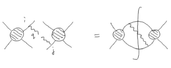
Figure 1: Soft gluon emission (wavy line) off a four-parton hard scattering.

We’ll start with a very brief review of soft gluons. The Feynman rule for the emission of a soft gluon off any fast parton is, to good approximation, proportional to the four-momentum of the fast parton. This simplification means that we can factorize the cross-section for an $n+1$ parton process (i.e. with one soft gluon and $n$ partons participating in the hard scatter) as

$$\mathrm{d}\sigma_{n+1}=\mathrm{d}\sigma_{n}\frac{\alpha_{s}}{2\pi}\frac{\mathrm{d}E}{E}\frac{\mathrm{d}\Omega}{2\pi}\sum_{ij}C_{ij}E^{2}\frac{p_{i}\cdot p_{j}}{p_{i}\cdot q\;p_{j}\cdot q}$$ (1)

where the various symbols are defined (for $n=4$) in Fig. 1. The blob in the figure represents a generic short-distance process and we need only ever consider soft gluon emissions off external legs since they are incapable of putting the internal hard propagators on-shell. The virtual corrections factorize similarly, and we will have more to say about them shortly. All looks pretty simple, but there is a major obstacle preventing automated soft gluon calculations in generic processes: the colour factor $C_{ij}$ is very difficult to keep track of. Think of emitting many soft gluons. The leading logarithmic behaviour nests, which means that each emission sees an effective short-distance process involving all previous emissions and the corresponding colour structure lives in some large representation of SU(3). This actually is no problem for theorists who can calculate in a colour basis independent way [1, 2] but it is a problem when it comes to putting a number on a cross-section. To date, this problem has not been solved for $n>3$. Monte Carlo generators, like HERWIG and PYTHIA, duck the issue by working in the large $N_{c}$ approximation. They also exploit the fact that, after integrating over azimuth in Eq. (1), soft emissions take place into cones of successively smaller angles as one moves away from the hard scatter. The major part of this talk will be concerned with soft gluons but a word first on collinear emissions.

Collinear partonic evolution is easier to deal with. The colour structure simplifies and partonic evolution reduces to a classical branching process: it is as if particles are emitted off the parton to which they are collinear. Hence (after integrating over azimuthal angle)

$$\mathrm{d}\sigma_{n+1}=\mathrm{d}\sigma_{n}\frac{\alpha_{s}}{2\pi}\frac{\mathrm{d}q^{2}}{q^{2}}\mathrm{d}z\sum_{ab}P_{ba}(z)$$ (2)

for $a\to bc$, where parton $b$ carries a fraction $z$ of parton $a$’s momentum, and $P_{ba}(z)$ is the corresponding splitting function.

The large $N_{c}$ approximation for soft emissions permits one to combine them with collinear emissions in a single parton shower, successive emissions being ordered in angle. Our task is to go beyond the leading $N_{c}$ approximation and gain a better understanding of soft gluon physics.

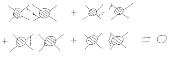
Figure 2: Soft gluons cancel in a sum over cuts.

Fig. 2 is a diagrammatic statement of the Bloch-Nordsieck Theorem: Summing over cuts, the real and virtual contributions exactly cancel in the soft gluon approximation. If real emissions are forbidden for some reason (or contribute to an observable with anything other than unit weight) then a miscancellation is induced and that leaves behind a logarithm in the volume $V$ of the phase-space into which real emission is suppressed. Examples of observables affected in this way are event shapes (e.g. thrust where $V=1-T$), production near threshold ($V=1-M^{2}/s$), Drell-Yan at low $p_{T}$ ($V=p_{T}^{2}/s$), deep inelastic scattering at large $x$ ($V=1-x$) and “gaps between jets”. Our attention now turns to the latter process: it is the simplest process involving four partons in the hard scatter. Specifically, one is interested in a final state containing two high $p_{T}$ jets. The observable cross-section is defined by imposing that there be no additional jets in the rapidity region between the two hard jets that have $p_{T}>Q_{0}$. We emphasise that $Q_{0}$ defines the gap in an experimentally well defined manner [3, 4]. For this observable $V=Q_{0}/Q$ where $Q$ is the $p_{T}$ of the hard jets.

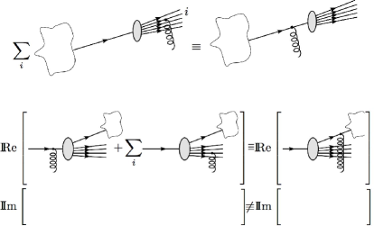
Figure 3: Coherence.

QCD coherence underpins the angular ordering of soft gluon emissions and can be used to argue that a wide-angle soft gluon emitted off a bunch of collinear partons can always be re-attached to the primary hard parton that defines the direction of the bunch. It is a statement at the amplitude level for the virtual soft gluon corrections and is illustrated in Fig. 3. It is understood that there are any number of additional partons exiting the hard-scatter blob (not shown) and that the soft gluon re-attaches to one of them. The crucial point to note is that coherence defined in this diagrammatic sense breaks down for the imaginary part of the amplitude. It is spoilt by virtual soft gluons that put on-shell the partons to which they attach. Such gluons are variously called Coulomb or Glauber gluons in the literature and they are the bane of those wanting to prove QCD factorization theorems. Assuming coherence leads us to conclude that the gaps-between-jets observable should contain only single logarithms, i.e. terms $\sim\alpha_{s}^{n}\ln^{n}(Q/Q_{0})$, since it is inclusive over the collinear regions.

Figure 4: The soft gluon dressing of a two-parton process.

2 Pre 2001: Exponentiation

We start with the simplest example: $e^{+}e^{-}\to q\bar{q}$ with a restriction $p_{T}<Q_{0}$ on the emission of additional jets into a region of rapidity $Y$ somewhere in between the primary jets. Naively, we need only compute the diagram shown in Fig. 4, where the blob represent the short distance physics. The soft gluon should be integrated over the region into which real emissions are forbidden. In particular, the real part of this one-loop amplitude should be integrated over rapidities in the gap and $k_{T}>Q_{0}$ since the complementary region is cancelled by real emissions according to Bloch-Nordsieck. We refer to the soft gluons that generate this real part as eikonal gluons. The imaginary part is more subtle: it arises as a result of Coulomb gluon exchange and has nothing to cancel against (it makes no sense to speak of the rapidity of these gluons). To pick up all of the leading logarithms to all orders in $\alpha_{s}$ one might think that we need only iterate the process of adding a soft gluon between the jets, with each successive emission occurring at much smaller $k_{T}$ than the one before. It is as if all prior emissions are sitting in the short-distance blob in Fig. 4. The net effect is an amplitude

$$A = A_{0}\exp\left(-\frac{\alpha_{s}}{\pi}\int_{Q_{0}}^{Q}\frac{\mathrm{d}k_{t}}{k_{t}}C_{F}(Y+\rho_{\mathrm{jet}})\right)$$ (3)

$$\times \exp\left(+\frac{2\alpha_{s}}{\pi}\int_{0}^{Q}\frac{\mathrm{d}k_{t}}{k_{t}}C_{F}\;i\pi\right)~{},$$

where $\rho_{\mathrm{jet}}$ is some function dependent upon the jet algorithm (we have ignored the running of the coupling but it is easy enough to restore it). The colour structure in this two-jet example is simple (the $q\bar{q}$ must be in a colour singlet) and as a result the Coulomb gluon ($i\pi$) term generates an unimportant phase.

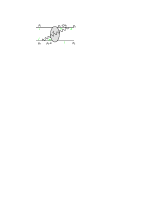
Figure 5: The soft gluon dressing of a four-parton process.

The story is much the same for three and four-parton processes. In hadron-hadron collisions we need to compute the virtual corrections illustrated in Fig. 5. These are the leading diagrams at large $Y$ and there are two others (where the soft gluon links partons 1 and 3 or partons 2 and 4), which contribute only to the dependence upon $\rho_{\mathrm{jet}}$. The only subtlety arises because the colour structure is now not so simple. For quark-quark scattering one can think of projecting the amplitude onto a specific basis and the soft gluons can generate mixing. The result is an amplitude that goes as

$$\mathbf{A}=\exp\left(-\frac{2\alpha_{s}}{\pi}\int_{Q_{0}}^{Q}\frac{\mathrm{d}k_{t}}{k_{t}}\boldsymbol{\Gamma}\right)\mathbf{A}_{0}~{}.$$ (4)

In the $t$-channel singlet-octet basis (e.g. the top left entry generates pure singlet evolution):

$$\mathbf{\Gamma}=\left(\begin{array}[]{cc}\frac{N^{2}-1}{4N}\rho_{\mathrm{jet}}&\frac{\sqrt{N^{2}-1}}{2N}i\pi\\ \frac{\sqrt{N^{2}-1}}{2N}i\pi&-\frac{1}{N}i\pi+\frac{N}{2}Y+\frac{N^{2}-1}{4N}\rho_{\mathrm{jet}}\end{array}\right)$$ (5)

and $\sigma=\mathbf{A}^{\dagger}\mathbf{A}$. Now the Coulomb gluons don’t only lead to a phase: witness the $i\pi$ terms in the evolution matrix. The inclusive nature of the region $k_{t}<Q_{0}$ does however mean that they cancel in that region since the evolution is determined by a purely imaginary matrix, i.e. $\Im\mathrm{m}\;\boldsymbol{\Gamma}$. Hence the universal lower cut-off of $Q_{0}$. The calculation of these Sudakov logarithms in all $2\to 2$ sub-processes can be found in [5, 6].

Although we have been focussing our attention on gaps-between-jets, it is worth recalling that the formalism carries over almost without change to the case when a colour singlet particle(s) is produced in between the jets (e.g. a Higgs boson) since the soft gluon evolution is blind to it. The only change occurs in the jet function because the final state jets now recoil against the Higgs [7]. Notice that any studies of a jet veto in Higgs-plus-two-jets that are performed using the general purpose Monte Carlos necessarily miss the effects of Coulomb gluons and hence any singlet-octet mixing. This is a particularly serious deficiency at large $Y$ and for stringent vetos, where colour singlet exchange will eventually dominate.

3 2001-2006: Non-global logarithms

The exponentiation of soft gluons is not the whole story. In 2001, Dasgupta & Salam [8, 9] realized that a whole tower of leading logarithms was being neglected. Fig. 6 illustrates the problem.

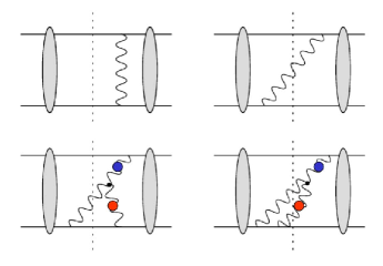
Figure 6: The origin of non-global logarithms.

The top two panes illustrate the real-virtual cancellation of Bloch-Nordsieck and the bottom two illustrate the problem. The blue (darker) blob indicates a soft gluon that is emitted outside of the gap but with $p_{T}>Q_{0}$. In the left picture, it receives a virtual correction from the red gluon, which necessarily has a lower $p_{T}$ but is still above $Q_{0}$. Crucially, this red gluon can be in the gap region. The right picture represents the real emission that would cancel the aforementioned virtual correction in a sufficiently inclusive observable. However, the real emission diagram is forbidden by the gap definition (since the red gluon is “in the gap and has $p_{T}>Q_{0}$”), which means that the virtual correction on the left has nothing to cancel against. Clearly the argument applies to any number of real emissions outside of the gap and instead of being able to focus only on virtual corrections to the primary hard scatter we now have to contemplate amplitudes with arbitrary numbers of real emissions and the virtual corrections to them. That is clearly a tall order and, to date, these leading “non-global” logarithms have only been summed up to all orders within the leading $N_{c}$ approximation and in the case of two-parton observables. Physical insight into this effect can be gained by noting that the all-orders result is essentially that, by requiring the gap region to be free of radiation above $Q_{0}$, a region outside it must also be depopulated, named the buffer zone in [9]. A very interesting feature worth mentioning is that the equation that sums these logarithms [11] is identical in form to the Balitsky-Kovchegov equation [12, 13] in small-$x$ physics [14, 15]. Is this coincidence or does it reflect a deeper connection between high energy scattering amplitudes and jet physics? The physics behind non-global logarithms is almost embarrasingly simple: the observable is obviously sensitive to the fact that emissions outside of the gap cannot emit back into the gap.

4 Post 2006: Super-leading logarithms?

As a first step to understanding non-global logarithms we decided to compute the tower of leading non-global logarithms that arise as a result of one gluon sitting outside the gap [16]. One might view this as the first term in an expansion in the number of out-of-gap gluons and it has the virtue that we can go ahead and calculate the cross-section without making the large $N_{c}$ approximation. To make progress we need two new ingredients: (i) we need to know how to emit a real (soft) gluon off the four-parton amplitude; (ii) we need to be able to dress the resulting five-parton amplitude with a virtual soft gluon.

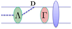
Figure 7: Five-parton evolution.

Fig. 7 illustrates schematically how the five-parton matrix element is computed. Assuming that successive emissions occur at progressively lower $k_{T}$, starting from the hard scatter at scale $Q$ (on the right in the figure), the general amplitude contains first a period of virtual evolution, which is carried out by successive operations of the four-parton evolution matrix $\boldsymbol{\Gamma}$, followed by the emission of a real gluon (denoted by $\mathbf{D}$ in the figure) and this in turn is followed by a period of five-parton evolution (denoted by $\boldsymbol{\Lambda}$). Kyrieleis & Seymour computed $\mathbf{D}$ and $\boldsymbol{\Lambda}$ for four-quark amplitudes [17] and Sjödahl recently computed the remaining five parton evolution matrices in a specific colour basis [18]. It is also possible to write down the evolution matrix for a general $n$-parton amplitude in a basis-independent manner [1, 2]. The result is (with a particular choice of the overall phase):

$$\mathbf{\Gamma} = \frac{1}{2}Y\mathbf{T}_{t}^{2}+i\pi\mathbf{T}_{1}\cdot\mathbf{T}_{2}+\frac{1}{4}\sum_{i\in F}\rho_{\mathrm{jet},i}\;\mathbf{T}_{i}^{2}$$ (6)

$$+ \frac{1}{2}\sum_{(i<j)\in L}\lambda_{\mathrm{jet},ij}\;\mathbf{T}_{i}\cdot\mathbf{T}_{j}$$

$$+ \frac{1}{2}\sum_{(i<j)\in R}\lambda_{\mathrm{jet},ij}\;\mathbf{T}_{i}\cdot\mathbf{T}_{j}~{}.$$

$\mathbf{T}_{i}$ is the colour charge of parton $i$ (partons 1 and 2 are incoming and the others are outgoing) and $\mathbf{T}_{t}$ is the net charge exchanged in the $t$-channel, i.e. $\mathbf{T}_{t}=\sum_{i\in L}\mathbf{T}_{i}=-\sum_{i\in R}\mathbf{T}_{i}$ and the sums are over all incoming and outgoing partons lying on either the left or right side of the gap. Notice that the terms involving $\rho_{\mathrm{jet},i}$ are Abelian since $\mathbf{T}_{i}^{2}=C_{F}\boldsymbol{1}$ or $C_{A}\boldsymbol{1}$ depending upon whether parton $i$ is a quark/antiquark or gluon. $\lambda_{\mathrm{jet},ij}$ is a second jet function.

Now $\mathbf{\Gamma}$ has a very important property: it is safe against final state collinear singularities. More specifically, if any two or more partons in the final state become collinear with each other, the soft gluon evolution of the system is identical to the evolution of the system in which the collinear partons are replaced by a single parton with the same total colour charge. That is, if $k$ and $l$ are the collinear partons, then $\mathbf{\Gamma}$ depends only upon $\mathbf{T}_{k}+\mathbf{T}_{l}$ and not upon the $\mathbf{T}_{k}$ or $\mathbf{T}_{l}$ separately. A proof can be found in [2] and results in the factorization expressed in the upper diagram of Fig. 3. This is to be contrasted with the initial state collinear limit, i.e. in which one or more outgoing partons becomes collinear with one of the incoming partons. The proof clearly breaks down for the imaginary part because of the Coulomb gluon term $i\pi\mathbf{T}_{1}\cdot\mathbf{T}_{2}$, which depends only on the colours of the initial state partons and not on the sum of the colour charges of the collinear partons. As a result the factorization is broken, as illustrated in the lower part of Fig. 3. It is this breakdown of naive coherence that leads directly to the appearance of super-leading logarithms in the calculation of the gaps-between-jets cross-section.

For one gluon outside of the gap the cross-section is thus

$$\sigma_{1}=-\frac{2\alpha_{s}}{\pi}\int_{Q_{0}}^{Q}\frac{dk_{T}}{k_{T}}\int_{\mathrm{out}}\frac{dy\,d\phi}{2\pi}\Bigl{(}\Omega_{R}+\Omega_{V}\Bigr{)},$$ (7)

where the integral is over the phase-space for the out-of-gap gluon and

$$\Omega_{V} = \mathbf{A}_{0}^{\dagger}\exp\left(-\frac{2\alpha_{s}}{\pi}\int_{Q_{0}}^{Q}\frac{dk_{T}^{\prime}}{k_{T}^{\prime}}\mathbf{\Gamma}^{\dagger}\right)$$ (8)

$$\exp\left(-\frac{2\alpha_{s}}{\pi}\int_{Q_{0}}^{k_{T}}\frac{dk_{T}^{\prime}}{k_{T}^{\prime}}\mathbf{\Gamma}\right)\boldsymbol{\gamma}$$

$$\exp\left(-\frac{2\alpha_{s}}{\pi}\int_{k_{T}}^{Q}\frac{dk_{T}^{\prime}}{k_{T}^{\prime}}\mathbf{\Gamma}\right)\mathbf{A}_{0}+\mathrm{c.c.},$$

$$\Omega_{R} = \mathbf{A}_{0}^{\dagger}\exp\left(-\frac{2\alpha_{s}}{\pi}\int_{k_{T}}^{Q}\frac{dk_{T}^{\prime}}{k_{T}^{\prime}}\mathbf{\Gamma}^{\dagger}\right)\mathbf{D}_{\mu}^{\dagger}$$ (9)

$$\exp\left(-\frac{2\alpha_{s}}{\pi}\int_{Q_{0}}^{k_{T}}\frac{dk_{T}^{\prime}}{k_{T}^{\prime}}\mathbf{\Lambda}^{\dagger}\right)$$

$$\exp\left(-\frac{2\alpha_{s}}{\pi}\int_{Q_{0}}^{k_{T}}\frac{dk_{T}^{\prime}}{k_{T}^{\prime}}\mathbf{\Lambda}\right)\mathbf{D}^{\mu}$$

$$\exp\left(-\frac{2\alpha_{s}}{\pi}\int_{k_{T}}^{Q}\frac{dk_{T}^{\prime}}{k_{T}^{\prime}}\mathbf{\Gamma}\right)\mathbf{A}_{0}.$$

For $\Omega_{R}$, this has the structure advertised in Fig. 7. $\Omega_{V}$ involves virtual corrections to the four-parton matrix element and $\boldsymbol{\gamma}$ adds the virtual out-of-gap gluon; after integrating over rapidity and azimuth it is equal to $\Re\mathrm{e}\;\mathbf{\Gamma}$ using Eq. (5).

Rather than numerically evaluate $\sigma_{1}$, we shall compute it in the particular case that the out-of-gap gluon is collinear to one of the incoming partons. Naively, the integral over the rapidity of the out-of-gap gluon yields a divergence (it can have arbitrarily large rapidity). Traditionally that would not pose any problem because colour coherence (and the “plus prescription”) would say that $\Omega_{R}+\Omega_{V}=0$ in this limit, however in light of our previous discussion we are interested to see how the “coherence breaking” Coulomb gluon contribution works out. We need to treat the collinear region with a little more care than we have done. In particular we must go beyond the soft gluon approximation in order to account for the fact that a gluon of $k_{T}>Q_{0}$ cannot have infinite rapidity and finite energy. We should instead treat the collinear region using the collinear (but not soft) approximation. The integral over rapidity ought then to be replaced by

$$\int\limits_{\text{out}}dy~{}~{}\left.\frac{d\sigma}{dyd^{2}k_{T}}\right|_{\text{soft}} \rightarrow$$

$$\int\limits^{y_{\text{max}}}dy~{}\left.\frac{d\sigma}{dyd^{2}k_{T}}\right|_{\text{soft}}+\int\limits_{y_{\text{max}}}^{\infty}dy~{}\left.\frac{d\sigma}{dyd^{2}k_{T}}\right|_{\text{collinear}}.$$

In this equation $y_{\text{max}}$ divides the regions in which the soft and collinear approximations are used and the dependence on it will cancel in the sum. Now we know that

$$\int\limits_{y_{\text{max}}}^{\infty}dy~{}\left.\frac{d\sigma}{dyd^{2}k_{T}}\right|_{\text{collinear}} =$$

$$\int\limits_{y_{\text{max}}}^{\infty}dy~{}\left(\left.\frac{d\sigma_{\text{R}}}{dyd^{2}k_{T}}\right|_{\text{collinear}}+\left.\frac{d\sigma_{\text{V}}}{dyd^{2}k_{T}}\right|_{\text{collinear}}\right)~{},$$

where the contribution due to real gluon emission is

$$\int\limits_{y_{\text{max}}}^{\infty}dy~{}\left.\frac{d\sigma_{\text{R}}}{dyd^{2}k_{T}}\right|_{\text{collinear}}~{} =$$ (12)

$$\int\limits_{0}^{1-\delta}dz\frac{1}{2}\left(\frac{1+z^{2}}{1-z}\right)\frac{q(x/z,\mu^{2})}{q(x,\mu^{2})}A_{\text{R}}$$

$$=\int\limits_{0}^{1-\delta}dz\frac{1}{2}\left(\frac{1+z^{2}}{1-z}\right)\left(\frac{q(x/z,\mu^{2})}{q(x,\mu^{2})}-1\right)A_{\text{R}}$$

$$+\int\limits_{0}^{1-\delta}dz\frac{1}{2}\frac{1+z^{2}}{1-z}A_{\text{R}}$$

and the contribution due to virtual gluon emission is

$$\int\limits_{y_{\text{max}}}^{\infty}dy~{}\left.\frac{d\sigma_{\text{V}}}{dyd^{2}k_{T}}\right|_{\text{collinear}} =$$ (13)

$$\int\limits_{0}^{1-\delta}dz\frac{1}{2}\left(\frac{1+z^{2}}{1-z}\right)A_{\text{V}}~{}.$$

In Eq. (12), $q(x,\mu^{2})$ is the parton distribution function for a quark in a hadron at scale $\mu^{2}$ and momentum fraction $x$. The factors $A_{\text{R}}$ and $A_{\text{V}}$ contain the $z$ independent factors which describe the soft gluon evolution and the upper limit on the $z$ integral is fixed since we require $y>y_{\text{max}}$:

$$\delta\approx\frac{k_{T}}{Q}\exp\left(y_{\text{max}}-\frac{\Delta y}{2}\right).$$ (14)

We are prepared for the fact that $A_{\text{R}}+A_{\text{V}}\neq 0$ (and we shall see it explicitly in Eq. (22)) but if it were the case that $A_{\text{R}}+A_{\text{V}}=0$ then the virtual emission contribution would cancel identically with the corresponding term in the real emission contribution leaving behind a term regularised by the ‘plus prescription’ (since we can safely take $\delta\rightarrow 0$ in the first term of Eq. (12)). This term could then be absorbed into the evolution of the incoming quark parton distribution function by choosing the factorisation scale to equal the jet scale $Q$.

The miscancellation therefore induces an additional contribution of the form

$$\int\limits_{0}^{1-\delta}dz\frac{1}{2}\left(\frac{1+z^{2}}{1-z}\right)(A_{\text{R}}+A_{\text{V}}) =$$

$$\ln\left(\frac{1}{\delta}\right)(A_{\text{R}}+A_{\text{V}})+\text{subleading}$$

$$\approx\left(-y_{\text{max}}+\frac{\Delta y}{2}+\ln\left(\frac{Q}{k_{T}}\right)\right)(A_{\text{R}}+A_{\text{V}}).$$

The $y_{\text{max}}$ dependence cancels with that coming from the soft contribution in Eq. (LABEL:eq:softcol) leaving only the logarithm. The leading effect of treating properly the collinear region is therefore simply to introduce an effective upper limit to the integration over rapidity in Eq. (7), i.e.

$$\int_{Q_{0}}^{Q}\frac{\mathrm{d}k_{T}}{k_{T}}\int_{\mathrm{out}}\mathrm{d}y \to$$ (16)

$$\int_{Q_{0}}^{Q}\frac{\mathrm{d}k_{T}}{k_{T}}\Bigg{(}\int^{y_{\mathrm{max}}}\mathrm{d}y+(-y_{\mathrm{max}}+\ln\frac{Q}{k_{T}})\Bigg{)}$$

$$=\frac{1}{2}\ln^{2}\frac{Q}{Q_{0}}.$$

In this way the super-leading logarithm emerges. We see that the non-collinear region is sub-leading and hence use the fact that, in the collinear limit, the evolution matrices simplify so that (neglecting an overall Abelian factor) the cross-section reduces to [2]

$$\sigma_{1} = -\frac{2\alpha_{s}}{\pi}\int_{Q_{0}}^{Q}\frac{dk_{T}}{k_{T}}\left(2\ln\frac{Q}{k_{T}}\right)$$ (17)

$$\Biggl{\langle}\!m_{0}\Biggr{|}e^{-\frac{2\alpha_{s}}{\pi}\int_{k_{T}}^{Q}\frac{dk_{T}^{\prime}}{k_{T}^{\prime}}\left(\frac{1}{2}Y\mathbf{t}_{t}^{2}-i\pi\mathbf{t}_{1}\cdot\mathbf{t}_{2}\right)}$$

$$\Biggl{\{}\mathbf{t}_{1}^{2}e^{-\frac{2\alpha_{s}}{\pi}\int_{Q_{0}}^{k_{T}}\frac{dk_{T}^{\prime}}{k_{T}^{\prime}}\left(\frac{1}{2}Y\mathbf{t}_{t}^{2}-i\pi\mathbf{t}_{1}\cdot\mathbf{t}_{2}\right)}$$

$$e^{-\frac{2\alpha_{s}}{\pi}\int_{Q_{0}}^{k_{T}}\frac{dk_{T}^{\prime}}{k_{T}^{\prime}}\left(\frac{1}{2}Y\mathbf{t}_{t}^{2}+i\pi\mathbf{t}_{1}\cdot\mathbf{t}_{2}\right)}$$

$$-\mathbf{t}_{1}^{a\dagger}e^{-\frac{2\alpha_{s}}{\pi}\int_{Q_{0}}^{k_{T}}\frac{dk_{T}^{\prime}}{k_{T}^{\prime}}\left(\frac{1}{2}Y\mathbf{T}_{t}^{2}-i\pi\mathbf{T}_{1}\cdot\mathbf{T}_{2}\right)}$$

$$e^{-\frac{2\alpha_{s}}{\pi}\int_{Q_{0}}^{k_{T}}\frac{dk_{T}^{\prime}}{k_{T}^{\prime}}\left(\frac{1}{2}Y\mathbf{T}_{t}^{2}+i\pi\mathbf{T}_{1}\cdot\mathbf{T}_{2}\right)}\mathbf{t}_{1}^{a}\Biggr{\}}$$

$$e^{-\frac{2\alpha_{s}}{\pi}\int_{k_{T}}^{Q}\frac{dk_{T}^{\prime}}{k_{T}^{\prime}}\left(\frac{1}{2}Y\mathbf{t}_{t}^{2}+i\pi\mathbf{t}_{1}\cdot\mathbf{t}_{2}\right)}\Biggl{|}m_{0}\!\Biggr{\rangle}.$$

We have changed to a bra-ket notation where $|m_{0}\rangle$ denotes the lowest order matrix element: it better suits the basis independent language wherein we are to think of the colour charges as objects that map vectors in $m$-parton colour space to vectors in $(m+1)$-parton colour space. Consequently, we have used lower ($\mathbf{t}_{i}$) and upper ($\mathbf{T}_{i}$) case symbols to represent the charge of parton $i$ in the four and five parton systems respectively. Note that it is the non-commutativity of $\mathbf{T}_{t}^{2}$ and $\mathbf{T}_{1}\cdot\mathbf{T}_{2}$ (and similarly $\mathbf{t}_{t}^{2}$ and $\mathbf{t}_{1}\cdot\mathbf{t}_{2}$) that prevents this expression from cancelling to zero: if they commuted then the two exponentials could be combined, all $\mathbf{T}_{1}\cdot\mathbf{T}_{2}$ and $\mathbf{t}_{1}\cdot\mathbf{t}_{2}$ dependence would cancel, $\mathbf{t}_{1}$ could be commuted through $\mathbf{T}_{t}^{2}$ and the real and virtual parts would be identical. For fewer than four external partons colour conservation means that we can always write $\mathbf{T}_{1}\cdot\mathbf{T}_{2}\propto\boldsymbol{1}$ and hence the Coulomb gluons only generate an unimportant phase.

We can get a better idea of what is going on if we expand the $\left\{...\right\}$ in Eq. (17) order by order in $\alpha_{s}$. By setting the exponentials to unity outside this bracket we are assuming that the out-of-gap gluon has the largest $k_{T}$ (we shall look at the other possibilities shortly). The first two orders vanish identically:

$$\Biggl{\{}\phantom{...}\Biggr{\}}_{0}=\mathbf{t}_{1}^{2}-\mathbf{t}_{1}^{a\dagger}\mathbf{t}_{1}^{a}=0.$$ (18)

$$\Biggl{\{}\phantom{...}\Biggr{\}}_{1}=-\frac{2\alpha_{s}}{\pi}\int_{Q_{0}}^{k_{T}}\frac{dk_{T}^{\prime}}{k_{T}^{\prime}}\Biggl{\{}\mathbf{t}_{1}^{2}Y\mathbf{t}_{t}^{2}-\mathbf{t}_{1}^{a\dagger}Y\mathbf{T}_{t}^{2}\,\mathbf{t}_{1}^{a}\Biggr{\}}$$ (19)

is also zero because

$$\mathbf{T}_{t}^{2}\,\mathbf{t}_{1}^{a}=\mathbf{t}_{1}^{a}\,\mathbf{t}_{t}^{2}.$$ (20)

Expanding to order $\alpha_{s}^{2}$ yields

$$\Biggl{\{}\phantom{...}\Biggr{\}}_{2} = \left(\frac{i\pi Y}{2}\right)\left(-\frac{2\alpha_{s}}{\pi}\int_{Q_{0}}^{k_{T}}\frac{dk_{T}^{\prime}}{k_{T}^{\prime}}\right)^{2}$$

$$\Biggl{\{}\mathbf{t}_{1}^{2}\left[\mathbf{t}_{t}^{2}\,,\mathbf{t}_{1}\cdot\mathbf{t}_{2}\right]-\mathbf{t}_{1}^{a\dagger}\left[\mathbf{T}_{t}^{2}\,,\mathbf{T}_{1}\cdot\mathbf{T}_{2}\right]\mathbf{t}_{1}^{a}\Biggr{\}}.$$

Note that this result comes only from the case where there is one Coulomb gluon and one eikonal gluon either side of the cut. Now, this term is not zero but the corresponding matrix element is zero, i.e. $\langle m_{0}|\left\{~{}\right\}_{2}|m_{0}\rangle=0.$

At the next order we obtain a non-zero result:

$$\!\Biggl{\{}\phantom{...}\Biggr{\}}_{3} \equiv -\frac{Y\pi^{2}}{6}\left(-\frac{2\alpha_{s}}{\pi}\int_{Q_{0}}^{k_{T}}\frac{dk_{T}^{\prime}}{k_{T}^{\prime}}\right)^{3}$$ (22)

$$\Biggl{\{}\mathbf{t}_{1}^{2}\Bigl{[}\left[\mathbf{t}_{t}^{2}\,,\mathbf{t}_{1}\cdot\mathbf{t}_{2}\right],\mathbf{t}_{1}\cdot\mathbf{t}_{2}\Bigr{]}$$

$$-\mathbf{t}_{1}^{a\dagger}\Bigl{[}\left[\mathbf{T}_{t}^{2}\,,\mathbf{T}_{1}\cdot\mathbf{T}_{2}\,\right],\mathbf{T}_{1}\cdot\mathbf{T}_{2}\Bigr{]}\mathbf{t}_{1}^{a}\Biggr{\}}.$$

Substituting back into Eq. (17), evaluating the colour matrix element and performing the transverse momentum integrals, we obtain a contribution to the first super-leading logarithm from configurations in which the out-of-gap gluon is hardest of

$$\sigma_{1,\mathrm{hardest}}=-\sigma_{0}\left(\frac{2\alpha_{s}}{\pi}\right)^{4}\ln^{5}\left(\frac{Q}{Q_{0}}\right)\pi^{2}Y\frac{N^{2}-2}{240}$$

in the case of $qq\to qq$. The other subprocesses lead to different colour matrix elements and hence a different coefficient of the form $(aN^{2}+b)$. The explicit results are presented in [2].

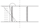
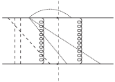
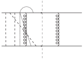
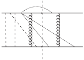
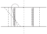
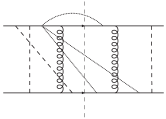
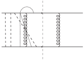
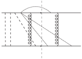
Figure 8: The relevant Feynman diagrams in the case that the out-of-gap (dotted) gluon is the hardest gluon. The dashed lines indicate soft (eikonal and Coulomb) gluons. Each subfigure represents three Feynman diagrams, corresponding to the three different ways of attaching the out-of-gap gluon. In diagrams (e) and (f) the soft gluon to the right of the cut should only be integrated over the region in which it has transverse momentum less than the out-of-gap gluon.

To complete the calculation of the order $\alpha_{s}^{4}$ super-leading logarithm we need to compute the contribution arising from the case where there is just one virtual emission of higher $k_{T}$ than the out-of-gap emission. Now we use the expression for $\{~{}\}_{2}$ derived in Eq. (4) in conjunction with the order $\alpha_{s}$ expansion of the exponential factors that lie outside of the main bracket in Eq. (17). Note that this is the only remaining contribution to the lowest order super-leading logarithm since all lower order expansions of the main bracket in Eq. (17) (i.e. $\{~{}\}_{1}$ and $\{~{}\}_{0}$) vanish. The result is

$$\sigma_{1,\mathrm{second-hardest}} =$$

$$-\sigma_{0}\left(\frac{2\alpha_{s}}{\pi}\right)^{4}\ln^{5}\left(\frac{Q}{Q_{0}}\right)\pi^{2}Y\frac{N^{2}-1}{120}.$$

At order $\alpha_{s}^{4}$ relative to the lowest order result, the total super-leading contribution to the gaps-between-jets cross-section for $qq\to qq$ arising from one soft gluon emission outside of the gap is therefore

$$\sigma_{1}=-\sigma_{0}\left(\frac{2\alpha_{s}}{\pi}\right)^{4}\ln^{5}\left(\frac{Q}{Q_{0}}\right)\pi^{2}Y\frac{3N^{2}-4}{240}.$$

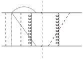
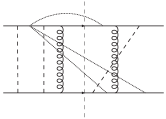
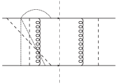
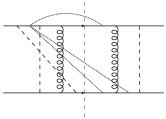
Figure 9: The relevant Feynman diagrams in the case that the out-of-gap (dotted) gluon is the second hardest gluon. The dashed lines indicate soft (eikonal and Coulomb) gluons. Each subfigure represents three Feynman diagrams, corresponding to the three different ways of attaching the out-of-gap gluon. The soft gluon to the right of the cut should only be integrated over the region in which it has transverse momentum less than the out-of-gap gluon.

Of the other sub-processes, the result for $qg\to qg$ is worth singling out because the size of the super-leading log does not depend upon whether the out-of-gap gluon is collinear to the quark or to the gluon.

5 Outlook

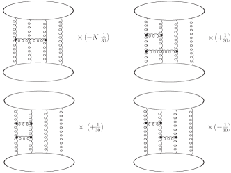
Figure 10: The four diagrams that generate the colour matrix elements when the out-of-gap gluon is the hardest gluon. In the case that the out-of-gap gluon is next-to-hardest, only the first diagram contributes. The upper and lower loops can be quarks, anti-quarks or gluons. Note that these are not Feynman diagrams or even uncut diagrams; they represent only the colour factor of the final result. In the first diagram one of the original six gluon lines has been contracted away, resulting in the additional factor of $N_{c}$.

The super-leading logarithms constitute a surprising breakdown of collinear factorization in an observable that sums inclusively over the collinear regions: the ‘plus prescription’ fails to operate and double (soft-collinear) logarithms make their appearance. The effect is due to Coulomb (Glauber) gluon exchange and it arises only in observables with at least four coloured partons in the hard scatter, is non-Abelian, sub-leading in $N_{c}$ and appears first at fourth order in the strong coupling relative to the lowest order. The implications for the gaps-between-jets cross-section are clear: collinear logarithms can be summed into the parton density functions only up to scale $Q_{0}$ and the logarithms in $Q/Q_{0}$ from further collinear evolution must be handled seperately. Moreover, since we now have a source of double logarithms, the calculation of the single logarithmic series necessarily requires knowledge of the two-loop evolution matrices [19, 20].

Some questions still remain open however: the structure of higher order super-leading logarithms; how widespread they are in other observables for hadron collisions; and whether they can be reorganized and resummed or removed by a suitable redefinition of observables or of incoming partonic states.

We close by noting that further simplifications are possible. In particular, the commutators between gluon exchanges from an external leg in different orders can be written as emission off the exchanged Coulomb gluons. The colour matrix elements can then be shown to be identical to those illustrated in Fig. 10. Once again it is clear that the super-leading logarithms arise as a result of the non-Abelian nature of the Coulomb gluon interaction. We also see that the coefficient of the superleading logarithm is independent of whether the out-of-gap gluon is collinear to parton 1 or 2, because the result is invariant under interchange of the particle types in the upper and lower loops. Colour structures like these are reminiscent of small-$x$ physics.

References

- [1] R. Bonciani, S. Catani, M. L. Mangano and P. Nason, Phys. Lett. B 575 (2003) 268 [arXiv:hep-ph/0307035].
- [2] J. R. Forshaw, A. Kyrieleis and M. H. Seymour, JHEP 0809 (2008) 128 [arXiv:0808.1269 [hep-ph]].
- [3] C. Adloff et al. [H1 Collaboration], Eur. Phys. J. C 24 (2002) 517 [arXiv:hep-ex/0203011].
- [4] S. Chekanov et al. [ZEUS Collaboration], arXiv:hep-ex/0612008.
- [5] G. Oderda and G. Sterman, Phys. Rev. Lett. 81 (1998) 3591 [arXiv:hep-ph/9806530].
- [6] C. F. Berger, T. Kucs and G. Sterman, Phys. Rev. D 65 (2002) 094031 [arXiv:hep-ph/0110004].
- [7] J. R. Forshaw and M. Sjödahl, JHEP 0709 (2007) 119 [arXiv:0705.1504 [hep-ph]].
- [8] M. Dasgupta and G. P. Salam, Phys. Lett. B 512 (2001) 323 [arXiv:hep-ph/0104277].
- [9] M. Dasgupta and G. P. Salam, JHEP 0203 (2002) 017 [arXiv:hep-ph/0203009].
- [10] R. B. Appleby and M. H. Seymour, JHEP 0309 (2003) 056 [arXiv:hep-ph/0308086].
- [11] A. Banfi, G. Marchesini and G. Smye, JHEP 0208 (2002) 006 [arXiv:hep-ph/0206076].
- [12] I. Balitsky, Nucl. Phys. B 463 (1996) 99 [arXiv:hep-ph/9509348].
- [13] Y. V. Kovchegov, Phys. Rev. D 60, 034008 (1999) [arXiv:hep-ph/9901281].
- [14] G. Marchesini and A. H. Mueller, Phys. Lett. B 575 (2003) 37 [arXiv:hep-ph/0308284].
- [15] H. Weigert, Nucl. Phys. B 685 (2004) 321 [arXiv:hep-ph/0312050].
- [16] J. R. Forshaw, A. Kyrieleis and M. H. Seymour, JHEP 0608 (2006) 059 [arXiv:hep-ph/0604094].
- [17] A. Kyrieleis and M. H. Seymour, JHEP 0601 (2006) 085 [arXiv:hep-ph/0510089].
- [18] M. Sjödahl, JHEP 0812, 083 (2008) [arXiv:0807.0555 [hep-ph]].
- [19] S. Mert Aybat, L. J. Dixon and G. Sterman, Phys. Rev. Lett. 97, 072001 (2006) [arXiv:hep-ph/0606254].
- [20] S. Mert Aybat, L. J. Dixon and G. Sterman, Phys. Rev. D 74 (2006) 074004 [arXiv:hep-ph/0607309].