Multiple regimes of diffusion

Abstract

We consider the diffusion of independent particles experiencing random accelerations by a space- and time-dependent force as well as viscous damping. This model can exhibit several asymptotic behaviours, depending upon the limiting cases which are considered, some of which have been discussed in earlier work. Here we explore the full space of dimensionless parameters, and introduce an ‘asymptotic phase diagram’ which delineates the limiting regimes.

I Introduction

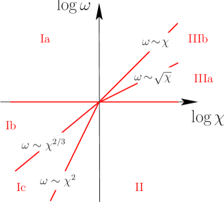
Figure 1: Phase diagram (schematic) for the model (2-4) summarising the different dynamical behaviours of Eq. (2) described in sections III-V: I Ornstein-Uhlenbeck, II generalised Ornstein-Uhlenbeck, IIIb overdamped minimum tracking, IIIa underdamped minimum tracking. The Ornstein-Uhlenbeck regime is divided into three regions: overdamped advection (Ia), underdamped advection (Ib), and underdamped inertial dynamics (Ic).

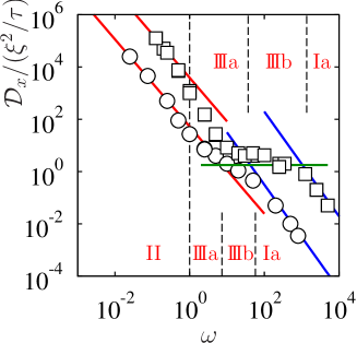
Figure 2: Illustration of multiple regimes of diffusion. Evaluation of the diffusion constant ${\cal D}_{x}$ for constant $\chi$ as a function of $\omega$: for $\chi=50$ (circles) and $\chi=1250$ (squares). Also shown is the expected behaviour in the advective limit, Ia, (blue) and the expected behaviour in regime II, ${\cal D}_{x}\sim\xi^{2}/\tau\,\,\chi^{4/3}\omega^{-5/3}$ (red). Finally, the estimate (42) for ${\cal D}_{x}$ in the minimum-tracking regime is shown (green line).

The position $x$ of a particle subjected to a force which fluctuates randomly in time $t$ might be expected to undergo diffusion, in the sense that

$$\lim_{t\to\infty}\frac{\langle x^{2}(t)\rangle}{2t}={\cal D}_{x}$$ (1)

for some diffusion coefficient ${\cal D}_{x}$, provided that there is some damping mechanism preventing the particle from being accelerated to arbitrarily high velocities. In this paper we determine the diffusion constant for the simplest model for this process in one spatial dimension, in which the equation of motion of the particle is

$$m\dot{x}=p\ ,\quad\dot{p}=-\gamma p+f(x,t)\,.$$ (2)

Here $x$ and $p$ are particle position and momentum, respectively, $m$ is the mass, and $\gamma$ is the rate at which the particle momentum is damped due to viscous drag. Time derivatives are denoted by dots. Further, the random forcing $f(x,t)$ is modeled by a Gaussian random function with zero mean and with correlation function $C(x,t)$, characterised by a correlation length $\xi$, correlation time $\tau$, and of typical size $\sigma$:

$$\langle f(x,t)\rangle=0\,,\quad\langle f(x,t)\,f(x^{\prime},t^{\prime})\rangle={C}(x\!-\!x^{\prime},t\!-\!t^{\prime})$$ (3)

(angular brackets denote averages). The dynamics of the model (2), (3) is determined by five dimensional parameters: $\sigma$, $\tau$, $\xi$, the mass $m$, and $\gamma$. Out of these one can form two independent dimensionless parameters: a dimensionless force $\chi=\sigma\tau^{2}/(m\xi)$ and a dimensionless damping $\omega=\gamma\tau$. In the following we explore the full space of dimensionless parameters $\chi$ and $\omega$.

There is no exact expression for the diffusion constant for this simple model. However, asymptotic expressions with different regions of validity are known, depending on which ratios of dimensionless parameters, $\omega$ and $\chi$, approach zero. We show that there are surprisingly many different asymptotic regimes, which are summarised in an ‘asymptotic phase diagram’, Fig. 1. The axes in this diagram are logarithms of two independent dimensionless parameters of the model, and a ray from the origin with slope $\nu$ represents a limiting process where $\chi$ approaches $0$ or $\infty$ with $\omega\sim\chi^{\nu}$. The phase lines do not indicate sharp transitions, but rather the boundaries between the domains of validity of six different asymptotic regimes as the limit is taken. Some of the regimes are well understood, but others are either new or have only been studied recently by the authors of this paper. It is remarkable that the phase diagram of such a fundamental model for diffusion processes has not been completely characterised before now. In all cases the long-time dynamics is diffusive, but in some of the regimes the stationary distribution of momentum may be strongly non-Gaussian, and the short-time behaviour may exhibit anomalous diffusion. The diffusion constant ${\cal D}_{x}$ depends in different ways on the microscopic parameters in different regimes, as illustrated in Fig. 2.

The three-dimensional version of the model defined by Eqs. (2) and (3) arises naturally in the study of small particles suspended in a randomly moving fluid, for which motion relative to the fluid is determined by viscous drag. In that context the random force is replaced by a random vector field, which would usually be chosen to be solenoidal, to represent an incompressible flow. This three-dimensional system has been extensively studied in certain limits. A significant early contribution is due to Maxey Maxey (1987), who analysed the clustering of particles suspended in a turbulent fluid (referred to as ‘preferential concentration’). Ref. Wilkinson et al. (2007) provides an overview of the literature on this problem, and describe recent progress.

This present paper is the first to explore the full range of regimes which are possible in limiting cases of the model, some of which are not realised in fluid-dynamical applications. We remark that different choices of dimensionless parameters are used in some other papers: much of the fluid dynamics literature uses the Stokes number ${\rm St}=1/\omega$ as a measure of the damping, and the Kubo number ${\rm Ku}=\chi/\omega$ as a measure of the time scale of fluctuations of the velocity field.

The model also exhibits an interesting effect which involves a phase transition in the conventional sense. Depending upon the dimensionless parameters of the model, particles with different initial conditions experiencing the same realisation of the random force approach the same trajectory with probability unity. This ‘path coalescence’ effect and the ‘path-coalescence transition’ where it disappears, were noted by Deutsch (1985), who appears to have been the first to consider this model systematically. In this paper we also describe the full phase line for the path-coalescence transition, extending results of Wilkinson & Mehlig (2003). The critical line for the path-coalescence transition in the $\chi$-$\omega$ plane is shown in Fig. 3.

The numerical simulations of Eqs. (2), (3) described in this paper were performed with the following choice of correlation function:

$$C(x,t)=\sigma^{2}\exp[-x^{2}/(2\xi^{2})-t^{2}/(2\tau^{2})]\,.$$ (4)

The detailed choice of the correlation function of the force is not significant, but in regime II, one aspect of the random forcing can make a qualitative difference. For any choice of the random force, there is a corresponding potential, satisfying $-\partial V(x,t)/\partial x=f(x,t)$. For a generic choice of correlation function, the one-dimensional potential $V(x,t)$ corresponding to the force $f(x,t)$ performs a random walk exhibiting increasing fluctuations as $|x|$ increases. We also consider cases where the particle dynamics is different if the potential $V(x,t)$ is a stationary random process.

The different regimes are illustrated in Fig. 4 by numerical simulations of the Eqs. (2-4). Shown are the trajectories $x(t)$ of several particles for a given realisation $f(x,t)$ of the forcing.

II Summary and physical description of the regimes

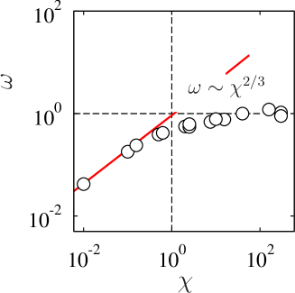
Figure 3: Phase line of the path-coalescence transition. Results of computer simulations of (2-4) for the phase line of the path-coalescence transition. Also shown is the theoretical result valid for small values of $\chi$, red line.

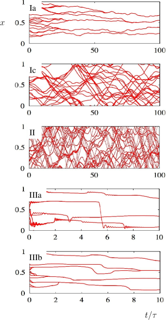
Figure 4: Trajectories $x(t)$ as a function of $t/\tau$ for $20$ particles with initial condition $p(0)=0$ and $x(0)$ randomly chosen in $[0,1]$. The first two pictures (in regimes Ia and Ic) are similar to those obtained by Deutsch (1985), and to Fig. 1 in (Wilkinson & Mehlig, 2003). The trajectories in region Ib are similar to those in Ia (not shown). The general difference in the dynamics of regimes IIIa and IIIb is that there are oscillations in regime IIIa, due to smaller damping.

Before describing our results in detail we discuss the physics of the parameter regimes of our model. We also mention connections with other work on the dynamics of randomly forced particles, where some of the regimes of our model have been studied.

One limiting case is where the particles are advected by a random velocity field: there is extensive literature on this problem and the closely related model of passive scalars (Falkovich et al., 2001). The advective case corresponds to regime Ia in our model.

Our model (2), (3) reduces to the well-known Ornstein-Uhlenbeck process (Ornstein and Uhlenbeck, 1930) when the position dependence of the force can be neglected. This is the case when the forcing is sufficiently weak so that the particle position changes negligibly within correlation time $\tau$: this condition will be made more precise below. The Ornstein-Uhlenbeck process is discussed in standard textbooks (see for example van Kampen (1981)). The regimes Ib,c can both be analysed by treating the evolution of the momentum as an Ornstein-Uhlenbeck process. The difference between the two regimes is that regime Ib exhibits path coalescence whereas regime Ic does not. Despite the fact that regime Ia describes an overdamped process, the formula for the diffusion constant is the same as for the Ornstein-Uhlenbeck process. For this reason regimes Ia and Ib,c are treated together in Sec. III, and are referred to as the Ornstein-Uhlenbeck regimes.

Our model is also related to stochastic or ‘Fermi’ acceleration of classical particles by random forces, which is used to model the production of cosmic rays (Fermi, 1949). In these studies the damping term (proportional to $\gamma$) is not included in the equation of motion, and the particle is accelerated to arbitrarily high energies. The treatment of the random forcing term in the case where the particle is rapidly moving, first considered in Sturrock (1966), is used in our consideration of regime II. Without damping the model exhibits anomalous diffusion (Golubovic, 1991; Rosenbluth, 1992). For the case where the damping term is included, a new dynamical regime was identified in Arvedson et al. (2006); Bezuglyy et al. (2006) with a non-Maxwellian velocity distributions (as well as anomalous diffusion at short times, before the damping term starts to limit the acceleration). This is regime II in the phase diagram Fig. 1: we call it the ‘generalised Ornstein-Uhlenbeck regime’. It is discussed in Sec. IV.

In the case where both the damping and the force are strong, the particle follows a local minimum of the potential $V(x,t)$. This is regime III of the phase diagram. This ‘minimum-tracking’ regime has not been considered in detail in earlier work. It is discussed in Sec. V below.

In Sec. VI we briefly describe how results for regime II differ for more general types of forcing, such as the case where $V(x,t)$ has stationary statistics.

Fig. 3 shows numerical results on the path-coalescence transition, for the choice of correlation function (4). For small values of $\chi$, the phase boundary is in precise agreement with an asymptotic theory discussed in Wilkinson & Mehlig (2003), which shows that the transition line is determined by the condition $\omega\chi^{-2/3}\to{\rm const.}$ in the limit as $\chi\to 0$. The data for large $\chi$ are consistent with the hypothesis that the phase line approaches $\omega={\rm const}.$ as $\chi\to\infty$, but we have no compelling argument to support this.

Finally, we comment on the physically accessible range of dimensionless parameters. This depends on the nature of the forcing. In the case of a particle suspended in a turbulent fluid flow with velocity field $u(x,t)$, the random forcing is due to viscous drag, and we write $f(x,t)=m\gamma u(x,t)$. In this case disturbances in the fluid velocity field $u(x,t)$ are transported by $u(x,t)$ itself. This implies that the Kubo number, ${\rm Ku}\equiv u\tau/\xi$ cannot be large (equivalently, $\chi$ cannot be large compared to $\omega$) if the random forcing is due to a fluid flow. In other cases, such as forcing by random electromagnetic fields, the entire phase diagram may be accessible.

III Ornstein-Uhlenbeck regime

We term the regimes Ia,b,c in the phase-diagram Fig. 1 the ‘Ornstein-Uhlenbeck regimes’. In these regimes, the particles move so slowly that the distance travelled during one correlation time $\tau$ of the random force $f(x,t)$ is much smaller than its correlation length $\xi$. Thus changes in the spatial argument do not contribute significantly to the decorrelation of $f(x,t)$ and one may approximate $f(x(t),t)\approx f(x(0),t)$ for times $t$ of the order of or less than the correlation time $\tau$.

Regime I is divided into one overdamped regime, regime Ia ($\omega\gg 1$) and two underdamped regimes Ib, c ($\omega\ll 1)$.

In the overdamped case, the acceleration term in eq. (2) is negligible, and consequently the particles are advected by the random force, that is, $\dot{x}\approx f(x,t)/(m\gamma)$. The two regimes Ib and Ic are distinguished by different behaviours of nearby particles, as can be seen in Fig. 4. In regime Ib, initially separate but nearby particle trajectories approach each other (path-coalescence regime). In regime Ic, by contrast, initially close particle trajectories do not coalesce.

In the remainder of this section we first briefly describe the single-particle dynamics (diffusion), and then summarise what is known about the path-coalescence transition.

To describe spatial diffusion in the overdamped regime, one integrates the advective equation of motion $\dot{x}=f(x,t)/(m\gamma)$. The change in position $\delta x$ during a short time interval $\delta t\gg\tau$ is

$$\delta x=\frac{1}{m\gamma}\int_{t}^{t+\delta t}{\rm d}t_{1}\ f\big{(}x({t_{1}}),t_{1}\big{)}\,.$$ (5)

In regime I, one may approximate $f(x({t_{1}}),t_{1})\approx f(x({t}),t_{1})$, as pointed out above. In this regime, the fluctuations of $f$ at a given point $x$ is indistinguishable from the fluctuations of $f$ along a particle trajectory. In this case it is straightforward to determine the fluctuations of $\delta x$: since the force is assumed to have vanishing mean (3), one has $\langle\delta x\rangle=0$. The variance of $\delta x$ is determined by making use of the fact that $\left<f(t)f(0)\right>$ is small unless $|t|<\tau$. Evaluating $\langle\delta x^{2}\rangle$ one finds the standard result

$$\langle\delta x^{2}\rangle=\frac{2D_{0}\delta t}{(m\gamma)^{2}}\,,$$ (6)

where $D_{0}$ is given by

$$D_{0}=\frac{1}{2}\int_{-\infty}^{\infty}{\mathrm{d}}t\left<f(t)f(0)\right>\,.$$ (7)

The position $x(t)$ at time $t=N\delta t$ of a particle after $N$ microscopic steps is $x(t)-x(0)=\sum_{i=1}^{N}\delta x^{(i)}$, where $\delta x^{(i)}$ is the increment at the time step number $i$. For the spatial diffusion constant one obtains in the usual fashion:

$${\cal D}_{x} = \lim_{t\to\infty}\frac{\left<(x(t)-x(0))^{2}\right>}{2t}$$

$$= \lim_{t\to\infty}\sum_{i,j=1}^{N}\frac{\left<\delta x^{(i)}\delta x^{(j)}\right>}{2\delta tN}=\frac{D_{0}}{(m\gamma)^{2}}\,,$$

where the increments $\delta x^{(i)}$ and $\delta x^{(j)}$ are statistically independent when $i\neq j$ and $\delta t\gg\tau$.

Consider now the underdamped regimes Ib, c. The displacements $\delta p$ of momentum (for a short time interval $\delta t$) obey

$$\delta p=-\gamma\,p\,\delta t+\delta w\,,$$ (9)

with

$$\delta w=\int_{t}^{t+\delta t}{\rm d}t_{1}\ f\big{(}x({t_{1}}),t_{1}\big{)}\,.$$ (10)

In regime I, the force fluctuates sufficiently rapidly compared to the time scale on which the momentum relaxes ($\omega\ll 1$) and the change $\delta p$ of momentum during one correlation time of the force is small compared to the typical value of $p$. Consequently (9) is a Langevin equation (van Kampen, 1981), describing the standard Ornstein-Uhlenbeck process where $\delta w$ is Gaussian distributed with

$$\langle\delta w\rangle=0\,,\quad\langle\delta w^{2}\rangle=2D_{0}\delta t\,.$$ (11)

From the corresponding Fokker-Planck equation for the distribution $P(p,t)$ of momentum $p$ at time $t$ (van Kampen, 1981)

$${\partial P\over{\partial t}}={\partial\over{\partial p}}\big{(}\gamma p+D_{0}{\partial\over{\partial p}}\big{)}P$$ (12)

one deduces that the steady-state distribution of momentum is Gaussian, $P(p)\propto\exp(-\gamma p^{2}/2D_{0})$.

Also in this underdamped regime the particles diffuse. The Fokker-Planck equation (12) allows to determine the correlation function of momentum in the steady state. The result is (van Kampen, 1981):

$$\left<p(t_{1})p(t_{2})\right>_{\rm steady\,\,state}=\frac{D_{0}}{\gamma}\exp(-\gamma|t_{2}-t_{1}|)\,.$$ (13)

This result in turn allows to calculate the spatial diffusion constant:

$${\cal D}_{x} = \lim_{t\to\infty}\frac{\left<x(t)^{2}\right>}{2t}$$

$$= \lim_{t\to\infty}\frac{1}{2tm^{2}}\int_{0}^{t}{\mathrm{d}}t_{1}\int_{0}^{t}{\mathrm{d}}t_{2}\left<p(t_{1})p(t_{2})\right>_{\rm steady\,\,state}$$

$$= \frac{D_{0}}{(m\gamma)^{2}}\,.$$

By comparing the results (III) and (III) one finds that the spatial diffusion constant is the same in the over- and the underdamped limits,

$${\cal D}_{x}=\frac{D_{0}}{(m\gamma)^{2}}\propto\frac{\xi^{2}}{\tau}\frac{\chi^{2}}{\omega^{2}}\,.$$ (15)

Fig. 2 shows results of numerical simulations for the diffusion constant of the model (2-4). In the Ornstein-Uhlenbeck regime (I) the simulations agree well with Eq. (15).

We now briefly summarise what is known about the path-coalescence transition which distinguishes regime Ib from Ic. In the path-coalescing phase (regime Ib), particle trajectories governed by the equation of motion (2) coalesce, whereas in regime Ic initially close particle trajectories separate almost surely (see Fig. 4). As was argued in Wilkinson & Mehlig (2003), the maximal Lyapunov exponent $\lambda$ serves as an ‘order parameter’ for the phase transition. The exponent describes the rate of change of an infinitesimal separation between two trajectories

$$\lambda=\lim_{t\to\infty}t^{-1}\log_{\rm e}\Big{|}\frac{\delta x_{t}}{\delta x_{0}}\Big{|}\,.$$ (16)

Here $\delta x_{0}$ is the initial separation of two infinitesimally close trajectories, and $\delta x_{t}$ is their separation at time $t$.

In regime Ib, the Lyapunov exponent is negative while it is positive in regime Ic. The condition for the phase transition is thus $\lambda=0$. In regime I, the Lyapunov exponent can be calculated exactly (Wilkinson & Mehlig, 2003). Expressed in terms of the dimensionless parameters $\chi$ and $\omega$, the phase transition is found to occur at

$$\omega\chi^{-2/3}={\rm const.}$$ (17)

Fig. 3 shows results of numerical simulations for the locus of the path-coalescence transition in the $\chi$-$\omega$-plane for the model (2-4). In regime I, the transition line is given by a line of slope $2/3$, as expected from (17).

To conclude this section, we briefly discuss the conditions delineating regime I in Fig. 1. First, in the overdamped limit, it was assumed that the distance covered in time $\tau$ is smaller than $\xi$. Estimating the advective velocity by $\sigma/(m\gamma)$ we have the condition $\sigma\tau/(m\gamma)\ll\xi$. Consequently the line distinguishing regimes Ia and IIIb is given by the condition that $\omega/\chi$ is of order unity. Second, in the underdamped limit, $\omega\ll 1$, the boundary between regimes Ic and II is parameterised by the condition that $\omega/\chi^{2}$ is of order unity. This condition is derived in the next section (Eq. (33)), where regime II is discussed.

IV Generalised Ornstein-Uhlenbeck regime

We term the regime II in the phase diagram Fig. 1 the ‘generalised Ornstein-Uhlenbeck regime’. This regime is defined by strong stochastic forcing: the particles move fast and their momenta can be much larger than $p_{0}=m\xi/\tau$. This means that the particle may travel many correlation lengths $\xi$ during one correlation time $\tau$ and the stochastic force acting on the particle may decorrelate quicker than $\tau$. Thus the ‘effective correlation time’ of the force $\xi m/\sqrt{\langle p^{2}\rangle}$ can be much smaller than $\tau$. It is also assumed that the dynamics of regime II is underdamped, i.e. $\omega\ll 1$.

A Fokker-Planck description is adequate in this regime. Define the increment $\delta w$ of the force for a small time interval $\delta t$

$$\delta w=\int_{t}^{t+\delta t}{\rm d}t_{1}\ f\big{(}x({t_{1}}),t_{1}\big{)}\,.$$ (18)

In regime I, the time dependence of $x(t_{1})$ could be neglected, but this approximation is no longer valid when the forcing is strong. Instead, one integrates the equation of motion (2) to obtain $x(t)=x(0)+\delta x$, where

$$\delta x\!=\!\frac{1}{m}\int_{0}^{t}\!\!{\mathrm{d}}t^{\prime}e^{-\gamma t^{\prime}}\Big{[}p(0)+\int_{0}^{t^{\prime}}\!\!{\mathrm{d}}t^{\prime\prime}e^{\gamma t^{\prime\prime}}f(x(t^{\prime\prime}),t^{\prime\prime})\Big{]}\,.$$ (19)

For times smaller than the small time interval $\delta t$, $\delta x$ is small and one may expand the force around $\delta x=0$. To lowest order in $\delta t$ one obtains

$$\left<\delta w\right> \approx \int_{0}^{\delta t}{\mathrm{d}}t_{1}\left<\frac{\partial f}{\partial x}(x(0),t_{1})\delta x\right>$$

$$\approx \frac{1}{m}\int_{0}^{\delta t}{\mathrm{d}}t_{1}\int_{0}^{t_{1}}{\mathrm{d}}t^{\prime}\int_{0}^{t^{\prime}}{\mathrm{d}}t^{\prime\prime}e^{-\gamma(t^{\prime}-t^{\prime\prime})}$$

$$\hskip 28.45274pt\times\left<\frac{\partial f}{\partial x}(x(0),t_{1})f(x(t^{\prime\prime}),t^{\prime\prime})\right>$$

where we have used that $\left<f(x(0),t)\right>=0$. Since it is assumed that $\omega=\gamma\tau\ll 1$, the exponent $\gamma(t^{\prime}-t^{\prime\prime})\approx 0$ and the major contribution to the integrals from the force correlation is for $|t_{1}-t^{\prime\prime}|<\tau$. We get

$$\left<\delta w\right>\approx\frac{\delta t}{2m}\int_{-\infty}^{\infty}{\mathrm{d}}t\,t\left<\frac{\partial f}{\partial x}(0,0)f(pt/m,t)\right>\,.$$ (21)

The variance of the displacements (18) becomes lowest order in $\delta t$

$$\left<\delta w^{2}\right> = \int_{0}^{\delta t}{\mathrm{d}}t_{1}\int_{0}^{\delta t}{\mathrm{d}}t_{2}\left<f\left(pt_{1}/m,t_{1}\right)f\left(pt_{2}/m,t_{2}\right)\right>$$ (22)

$$\approx \delta t\int_{-\infty}^{\infty}{\mathrm{d}}t\,C(pt/m,t)\,,$$

where $C$ is the correlation function of the force (3).

Using that the change $\delta p$ of momentum during a short time period is $\delta p=-\gamma p\delta t+\delta w$ together with the first two moments of $\delta w$ (Eqs. (21) and (22)), a Fokker-Planck equation is obtained using the standard procedure (van Kampen, 1981):

$${\partial P\over{\partial t}}={\partial\over{\partial p}}\left(-v(p)+{\partial\over{\partial p}}D(p)\right)P\,.$$ (23)

Here the drift- and diffusion-coefficients are

$$v(p) = \lim_{\delta t\to 0}\frac{\left<\delta p\right>}{\delta t}=-\gamma p+\frac{\partial}{\partial p}D(p)$$

$$D(p) = \lim_{\delta t\to 0}\frac{\left<\delta p^{2}\right>}{2\delta t}=\frac{1}{2}\int_{-\infty}^{\infty}{\mathrm{d}}t\,C(pt/m,t)\,,$$ (24)

where it was used that $\left<\delta w\right>=\delta t{\partial_{p}}D(p)$. The above expression for the diffusion constant was earlier obtained in Sturrock (1966), and has also been used in Golubovic (1991) and Rosenbluth (1992). Note that when $|p|\ll p_{0}$, $D(p)\approx D_{0}$, which corresponds to the Fokker-Planck equation of the standard Ornstein-Uhlenbeck process discussed in Sec. III.

On the other hand, when $|p|\gg p_{0}$ we approximate

$$D(p)\!=\!{D_{1}p_{0}\over|p|}+O(p^{-2})\,,\,D_{1}={m\over 2p_{0}}\int_{-\infty}^{\infty}\!\!\!\!\!\!{\rm d}X\ C(X,0)\,.$$ (25)

For the correlation function (4) we obtain $D(p)={D_{0}}/{(1+p^{2}/p_{0}^{2})^{1/2}}$, that is $D_{1}=D_{0}$.

If the force is the gradient of a potential $V(x,t)$ with continuous derivatives, $D_{1}$ vanishes and $D(p)\propto|p|^{-3}$ provided $V(x,t)$ is sufficiently differentiable. Further, if the correlation function exhibits a cusp at $t=0$ (an example is discussed by Bezuglyy et al. (2006)), we find $D(p)\propto|p|^{-2}$. In general we write

$$D(p)=D_{\zeta}\,\,\left(\frac{p_{0}}{|p|}\right)^{\zeta}$$ (26)

with $\zeta\geq 0$. In this paper we mainly discuss the case $\zeta=1$ which is a generic case for a random force [realised by the correlation function (4)]. But in Sec. VI we briefly mention what is known for other force models giving rise to $\zeta\neq 1$.

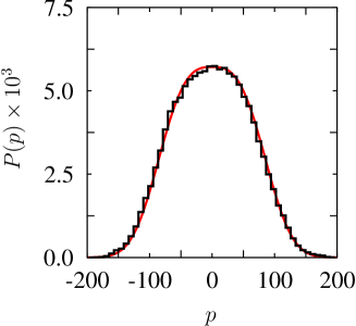
Figure 5: Non-Gaussian distribution of momentum in phase II (c.f. Fig. 1). Shown are results of numerical simulations of (2) for $\chi=50$ and $\omega=0.01$ compared with eq. (28).

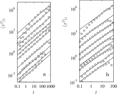
Figure 6: Shows $\langle x^{2}\rangle_{t}$ as a function of $t$; a $\chi=50$ and $\omega=0.025,0.075,0.25,0.5,1,2.5,50,200,500$ and $800$, from top to bottom; b $\chi=1250$ and $\omega=0.125,1,0.5,2.5,5,50,100,250,1250,2500$ and $5000$, from top to bottom. Solid lines are fits (as judged by the eye) to the diffusion law (1). The corresponding values of ${\cal D}_{x}$ are shown in Fig. 2.

The steady-state solution $P(p)$ of (23) is given by

$$P(p)=C\,\exp\Big{(}-\gamma\int_{0}^{p}{\rm d}p^{\prime}\frac{p^{\prime}}{D(p^{\prime})}\Big{)}\,.$$ (27)

where $C$ is chosen to normalise the distribution. When $D(p)\approx D_{0}$, the function $P(p)$ is approximately Gaussian, which corresponds to the standard Ornstein-Uhlenbeck regime (regimes Ib,c). When $D(p)=D_{1}p_{0}/|p|$, however, the distribution $P(p)$ is non-Gaussian (regime II): (Arvedson et al., 2006)

$$P(p)\sim\exp\Bigg{(}-\frac{\gamma|p|^{3}}{3p_{0}D_{1}}\Bigg{)}\,.$$ (28)

This result is compared to results of numerical simulations of Eqs. (2-4) in Fig. 5.

The generalised Ornstein-Uhlenbeck regime was studied in Ref. Arvedson et al. (2006), see also Ref. (Bezuglyy et al., 2006). The Fokker-Planck equation (23) was solved as an eigenvalue problem and the propagator to reach momentum $p$ at time $t$ given the initial momentum was found. From this propagator, the momentum correlation function at equilibrium was calculated

$$\left<p(t^{\prime})p(t^{\prime\prime})\right>_{\mathrm{e}q.} = \frac{\Gamma(4/3)}{3^{1/3}\Gamma(5/3)}\left(\frac{p_{0}D_{1}}{\gamma}\right)^{2/3}e^{-2\gamma|t^{\prime}-t^{\prime\prime}|}$$ (29)

$$\times F_{21}\left(\frac{1}{3},\frac{1}{3};\frac{5}{3};e^{-3\gamma|t^{\prime}-t^{\prime\prime}|}\right)\,,$$

where $F_{21}$ is a hypergeometric function (Abramowitz, 1972).

From the momentum correlation function (29) it is possible to calculate the spatial diffusion constant in regime II. The result is (Arvedson et al., 2006):

$${\cal D}_{x}\!=\frac{(p_{0}D_{1})^{2/3}}{m^{2}\gamma^{5/3}}\frac{\pi 3^{-5/6}}{2\,\Gamma\!(2/3)^{2}}F_{32}\Big{(}\frac{1}{3},\frac{1}{3},\frac{2}{3};\frac{5}{3},\frac{5}{3};1\Big{)}\,,$$ (30)

where $F_{32}$ is a hypergeometric function. Since $D_{1}\sim\sigma^{2}\tau$, the spatial diffusion constant ${\cal D}_{x}$ scales as

$${\cal D}_{x}\sim\frac{\xi^{2}}{\tau}\chi^{4/3}\omega^{-5/3}$$ (31)

as opposed to (15). Fig. 2 shows results of numerical simulations of the diffusion constant for the model (2-4) in this regime, in good agreement with eq. (30). The diffusion constant ${\cal D}_{x}$ was numerically determined by estimating $\langle x^{2}\rangle_{t}/(2t)$, according to Eq. (1). The corresponding data are shown in Fig. 6. The dynamics in the generalised Ornstein-Uhlenbeck regime exhibits anomalous diffusion at short times (Arvedson et al., 2006; Bezuglyy et al., 2006). Results of numerical experiments exhibiting anomalous diffusion are given in Arvedson et al. (2006).

To conclude this section we discuss the conditions under which the results described above are applicable. First we discuss the lines in Fig. 1 defining the limits of regime II. The discussion above assumes that the dynamics in regime II are described by a Fokker-Planck equation, (23), and we must also consider the conditions under which this equation is applicable.

Regime II is defined by the condition that the motion is underdamped, $\omega\ll 1$, and by the condition that the correlation time along the particle trajectory is smaller than the correlation time for a static particle. The latter condition defines the transition between regimes I and II in the phase diagram Fig. 1. This transition occurs when $\gamma p_{0}^{2}/D_{0}$ is of order unity. This fact is most easily seen by determining the steady-state distribution $P(p)$ of momentum for the particular form (4) of the correlation function: $P(p)=C\exp\big{(}-\frac{\gamma p_{0}^{2}}{3D_{0}}\big{[}(1+p^{2}/p_{0}^{2})^{3/2}-1\big{]}\big{)}$. In terms of the dimensionless parameters $\omega$ and $\chi$ the above condition becomes:

$${\gamma p_{0}^{2}\over D_{0}}\sim{\gamma m^{2}\xi^{2}\over{\sigma^{2}\tau^{3}}}=\frac{\omega}{\chi^{2}}={\rm const}\,.$$ (32)

Thus the lines distinguishing the boundaries of regime II in the phase diagram in Fig. 1 are

$$\omega=O(1)\quad\mbox{and}\quad\frac{\omega}{\chi^{2}}=O(1)\,.$$ (33)

Consider finally the conditions of validity of (23) in regime II. For a Fokker-Planck description of a stochastic process to be valid, two necessary conditions must hold

• Amplitude condition. The random jumps of the stochastic variable must be much smaller than its typical size. Therefore we must require that the change of momentum $\Delta p$ during a correlation time of the forcing is much smaller than $\sqrt{\langle p^{2}\rangle}$. This condition can be written in the form

  $$\frac{\Delta p}{p}\sim\frac{\sigma}{p}\frac{m\xi}{p}\sim\frac{\sigma m\xi}{{\langle p^{2}\rangle}} \sim \chi\Big{(}\frac{\omega}{\chi^{2}}\Big{)}^{2/3}\ll 1\,.$$ (34)

  Here we used the fact that the correlation time of the force is of the order of $m\xi/\sqrt{\langle p^{2}\rangle}$, and that in the steady state $\sqrt{\langle p^{2}\rangle}\sim(p_{0}D_{1}/\gamma)^{1/3}\sim p_{0}(\chi^{2}/\omega)^{1/3}$. The amplitude condition is thus fulfilled provided $\omega^{2}/\chi\ll 1$.

• Frequency condition. The stochastic forcing must fluctuate more rapidly than the stochastic variable. The correlation time of the force is of the order of $m\xi/\sqrt{\langle p^{2}\rangle}$, and the relaxation time of $p$ is of the order of $\gamma^{-1}$. We must therefore require that

  $$\frac{\gamma\xi m}{\sqrt{\langle p^{2}\rangle}}\sim\omega\Big{(}\frac{\omega}{\chi^{2}}\Big{)}^{1/3}\ll 1\ .$$ (35)

  The frequency condition thus amounts to the same condition as above.

In our model, the amplitude and frequency conditions may not be sufficient to ensure that (23) is valid. The reason is that the fluctuations experienced by the particle may be influenced by the random force altering the trajectory of the particle, so that the trajectory does not explore the random force field ergodically. In addition to the two conditions above the following self-consistency condition must also be satisfied:

• Self-consistency condition. It is required that in the steady state the particle moves sufficiently rapidly so that it is not captured by ‘valleys’ in the potential corresponding to $f(x,t)$:

  $$\langle p^{2}\rangle/(2m)\gg\xi\sigma\,.$$ (36)

  This condition too corresponds to $\omega^{2}/\chi\ll 1$.

Within the boundaries of region II we have $\omega\ll 1$ and $\omega/\chi^{2}\ll 1$. In this limit the condition $\omega^{2}/\chi\ll 1$ is always satisfied, so that the Fokker-Planck equation is in fact always applicable in regime II for the type of random force model with $\zeta=1$. In Sec. VI we shall see that this may not be true for other values of $\zeta$.

V Minimum-tracking regime

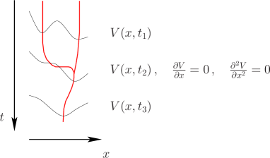
Figure 7: Disappearance of a minimum in $V(x,t)$ (black lines) and corresponding coalescence of particle trajectories (red lines, schematic).

We term the regimes III in the phase diagram Fig. 1 as the ‘minimum-tracking regimes’. These regimes are defined by large damping $\omega\gg 1$ and strong stochastic forcing $\chi/\omega\gg 1$. If the force had been weak, we would be in the advective regime Ia. When the force becomes large enough, the particle may get stuck in minima of the potential $V(x,t)=-\int_{0}^{x}\!\!{\rm d}x^{\prime}f(x^{\prime},t)$ of the force.

The minimum-tracking regimes are divided into two distinct dynamical regimes: under- and overdamped minimum-tracking. In the underdamped regime IIIa, the particle can oscillate around the potential minimum, whereas in the overdamped regime IIIb such oscillations are quickly damped out (Fig. 2).

In regime IIIb the diffusion constant is estimated as follows. Typically the particles are stuck in minima. As these minima randomly disappear and appear, the particle trajectories jump and may coalesce (Fig. 7). We argue that the diffusion constant is given in terms of the typical size of the valleys ($\xi$) and the rate at which they disappear. This rate can be estimated using a generalisation of the method discussed in Kac (1943); Rice (1945) for counting the zeroes of a random function $\mbox{\boldmath$F$}(\mbox{\boldmath$y$})$. According to Kac (1943), the density $\varrho$ of zeroes of the random function $\mbox{\boldmath$F$}(\mbox{\boldmath$y$})$ is given by

$$\varrho=\langle\delta(\mbox{\boldmath$F$})|\det{\bf G}|\rangle$$ (37)

with $G_{\alpha\beta}=\partial F_{\alpha}/\partial y_{\beta}$.

Valleys disappear at inflection points of $V(x,t)$, and we thus need to count the joint zeroes of $f$ and $\partial_{x}f\equiv f^{\prime}$:

$$\varrho=\langle\delta(f)\delta(f^{\prime})|\det{\bf G}|\rangle$$ (38)

with

$${\bf G}=\left(\begin{array}[]{ll}f^{\prime}&\frac{\partial f}{\partial t}\\[5.69054pt] f^{\prime\prime}&\frac{\partial f^{\prime}}{\partial t}\end{array}\right)\,.$$ (39)

We need to calculate the average with respect to the set of Gaussian random variables $a_{i}=\{f,f^{\prime},f^{\prime\prime},\partial_{t}f$,$\partial_{t}f^{\prime}\}$. The expectations of all five random variables vanish, and their covariances $\Sigma_{ij}$ can be expressed in terms of derivatives of the correlation function $C(x,t)$. For the special case (4) we obtain the covariance matrix

$$\mbox{\boldmath$\Sigma$}=\left(\begin{array}[]{ccccc}\sigma^{2}&0&-\sigma^{2}/\xi^{2}&&\\ 0&\sigma^{2}/\xi^{2}&0&&\\ -\sigma^{2}/\xi^{2}&0&3\sigma^{2}/\xi^{4}&&\\ &&&\sigma^{2}/\tau^{2}&\\ &&&&\sigma^{2}/(\xi^{2}\tau^{2})\end{array}\right)\,.$$ (40)

Performing the Gaussian average in (38), we obtain

$$\varrho=\frac{\sqrt{2}}{\pi^{2}}\frac{1}{\xi\tau}\,.$$ (41)

Note that this result is independent of $\sigma$. For the choice of correlation function (4), the density of minima of $V(x,t)$ for any given time is $(2\pi\xi)^{-1}$. Their typical separation is thus $2\pi\xi$. Assuming that particles jump by $2\pi\xi$ when their minima disappear, we arrive at the following estimate for the diffusion constant

$${\cal D}_{x}=\frac{1}{2}(2\pi)^{3}\frac{\sqrt{2}}{\pi^{2}}\frac{\xi^{2}}{\tau}=\sqrt{8}\pi\frac{\xi^{2}}{\tau}$$ (42)

This expression is in reasonable agreement with the results of numerical simulations shown in Fig. 2.

Now consider the conditions delineating regime IIIb. As $\omega$ is increased, regime Ia is entered from IIIb. The corresponding crossover line was determined in Sec. III, it is given by the condition that $\omega/\chi$ is of order unity. On the other hand, when $\omega$ is decreased, regime IIIa is entered, the underdamped minimum-tracking regime. The corresponding cross-over line is given by the condition

$$\gamma\omega_{\rm valley}\sim 1\,,$$ (43)

where $\omega_{\rm valley}=\sqrt{\sigma/(\xi m)}$ is the typical frequency of oscillation in the minimum. The above condition corresponds to

$$\omega^{2}/\chi={\rm const.}\,.$$ (44)

Both minimum-tracking regimes are on the path-coalescence side of the phase diagram Fig. 3, corresponding to negative Lyapunov exponent. Calculating this exponent is complicated by the fact that the minimum-tracking regimes are non-ergodic. However, in regime IIIa the Lyapunov exponent can be estimated as follows.

Making use of the fact that the particles are constrained to follow potential minima of the random force $f(x,t)$, expand the potential around a specific minimum at $x_{0}$ at a given time $t_{0}$, $V(x,t_{0})\approx V(x_{0},t_{0})+\frac{1}{2}V^{\prime\prime}(x_{0},t_{0})(x-x_{0})^{2}$. This gives $f=-{\partial_{x}V}\approx-C(x-x_{0})$, where $C=V^{\prime\prime}(x_{0},t_{0})>0$. In the vicinity of $x_{0}$, the equation of motion (2) becomes

$$m\dot{x}=p,\hskip 56.9055pt\dot{p}=-\gamma p-C(x-x_{0})\,.$$ (45)

Linearising for small separations $\delta x$ and $\delta p$ gives

$$\dot{\delta x}=\delta p/m,\hskip 56.9055pt\dot{\delta p}=-\gamma\delta p-C\delta x\,.$$ (46)

The dynamics of the separations is determined by the eigenvalues of the matrix

$${\bf A}=\left(\begin{array}[]{cc}0&1/m\\ -C&-\gamma\end{array}\right)\,.$$ (47)

The eigenvalues of ${\bf A}$ are

$$\lambda_{\pm}=-\frac{\gamma}{2}\pm\frac{\gamma}{2}\sqrt{1-\frac{4C}{m\gamma^{2}}}\,.$$ (48)

In regime IIIa, the discriminant in (48) is always negative (this follows from (44) and the fact that $C\sim\sigma/\xi$ which gives $C/m\gamma^{2}\sim\chi/\omega^{2}\gg 1$). In this regime, the real part of the eigenvalue, which describes the stability of the minimum, therefore always takes the value $-\gamma/2$. Because the real part of the eigenvalue is constant, we can conclude that the Lyapunov exponent in regime IIIa is $\lambda=-\gamma/2$.

Finally, as $\omega$ is reduced further, eventually region II is entered when the Lyapunov exponent turns positive. The phase line in Fig. 3 appears to be consistent with the path-coalescence transition occurring at $\omega={\rm const.}$. However, we have not been able to find an argument supporting this observation. Moreover, we have performed numerical simulations of the path-coalescence transition at large values of $\chi$ for random forces with correlations different from (4) and have found that the locus of the path-coalescence transition sensitively depends on the nature of the fluctuations of the force. This observation is in stark contrast to the boundary between regimes Ib,c where the scaling of the zero of the Lyapunov exponent is universal. This latter universality is illustrated by recent analytical results of Falkovich et al. (2007) (corresponding to regimes Ib,c) for a model where the force gradient is taken to be a piece-wise constant function (a so-called ‘telegraph process’).

VI A special case: generalised Ornstein-Uhlenbeck regime

Up to now we have considered the simplest case, where $f(x,t)$ is a Gaussian random function with a generic correlation function. For such a generic random force its potential function $V(x,t)$, defined by $f=-\partial V/\partial x$ executes a random walk, exhibiting increasing excursions as $|x|\to\infty$. This generic case corresponds to the case where $\zeta=1$ in (26). For general values of $\zeta$, the long-time diffusion coefficient and the law of anomalous short-time diffusion in regime II were calculated by Bezuglyy et al. (2006), where it was shown that a force derived from a statistically stationary potential corresponds to $\zeta=3$.

In this section we briefly discuss the conditions of validity for the Fokker-Planck equation (23) for general values of $\zeta$. The discussion follows that at the end of Sec. IV.

The three conditions to be satisfied are now:

• Amplitude condition. From (27) we find that the steady-state variance of momentum is $\langle p^{2}\rangle\sim(p_{0}D_{\zeta}/\gamma)^{-2/(2\zeta+1)}$. The amplitude condition is therefore:

  $$\frac{\Delta p}{p}\sim\frac{\sigma}{p}\frac{m\xi}{p}\sim\frac{\sigma m\xi}{{\langle p^{2}\rangle}} \sim \chi\Big{(}\frac{\omega}{\chi^{2}}\Big{)}^{2/(2\zeta+1)}\ll 1$$ (49)

• Frequency condition. In the steady state we require

  $$\gamma\xi m/\sqrt{\langle p^{2}\rangle}\sim\omega\Big{(}\frac{\omega}{\chi^{2}}\Big{)}^{1/(2\zeta+1)}\ll 1$$ (50)

• Self-consistency condition. For general values of $\zeta$, the self-consistency condition (36) yields

  $$\frac{2m\xi\sigma}{\langle p^{2}\rangle}\sim\chi\Big{(}\frac{\omega}{\chi^{2}}\Big{)}^{2/(2\zeta+1)}\ll 1\,.$$ (51)

  This is the same as (49).

For $\zeta=1$ these three conditions are equivalent and correspond to the condition $\omega^{2}/\chi\ll 1$ derived in Sec. IV. But for other values of $\zeta$, the conditions are no longer equivalent. Condition (51) can be written as

$$\omega\ll\chi^{3/2-\zeta}\,.$$ (52)

This corresponds to a line with slope $-(\zeta-\frac{3}{2})^{-1}$ in Fig. 1. For $\zeta<3/2$, this condition is satisfied everywhere in region II, and therefore does not pose an additional constraint on the validity of the Fokker-Planck equation (23). For $\zeta>3/2$, by contrast, is not satisfied everywhere in regime II; a new non-ergodic region appears in the phase diagram above the dividing line $\omega\chi^{-3/2+\zeta}=$const. We remark that the condition (50) is always satisfied in regime II.

Acknowledgments. This work was supported by Vetenskapsrådet (BM), and by the platform ‘Nanoparticles in an interactive environment’ at Göteborg university (KG, BM).

References

- Maxey (1987) M. R. Maxey, J. Fluid Mech., 174, 441-465, (1987).
- Wilkinson et al. (2007) M. Wilkinson, B. Mehlig, S. Östlund, and K. P. Duncan, Phys. Fluids, 19, 113303, (2007).
- Deutsch (1985) J. Deutsch, J. Phys. A: Math. Gen., 18, 1449, (1985).
- Wilkinson & Mehlig (2003) M. Wilkinson and B. Mehlig, Phys. Rev. E 68, 040101(R), (2003).
- Falkovich et al. (2001) G. Falkovich, K. Gawedzki, and M. Vergassola, Rev. Mod. Phys., 73, 913, (2001).
- Ornstein and Uhlenbeck (1930) G. E. Ornstein and L. S. Uhlenbeck, Phys. Rev., 36, 823, (1930).
- van Kampen (1981) N. G. van Kampen, Stochastic processes in physics and chemistry, 2nd ed., North-Holland, Amsterdam 1981.
- Fermi (1949) E. Fermi, Phys. Rev., 75, 1169, (1949).
- Sturrock (1966) P. A. Sturrock, Phys. Rev., 141, 186, (1966).
- Golubovic (1991) L. Golubovic, S. Feng, and F.-A. Zeng, Phys. Rev. Lett., 67, 2115, (1991).
- Rosenbluth (1992) M. N. Rosenbluth, Phys. Rev. Lett., 69, 1831, (1992).
- Arvedson et al. (2006) E. Arvedson, B. Mehlig, M. Wilkinson, and K. Nakamura, Phys. Rev. Lett., 96, 030601, (2006).
- Bezuglyy et al. (2006) V. Bezuglyy, B. Mehlig, M. Wilkinson, K. Nakamura, and E. Arvedson, J. Math. Phys., 47, 073301, (2006).
- Abramowitz (1972) M. Abramowitz and I. A. Stegun, Handbook of Mathematical Functions, 9th edition, Dover, New York, (1972).
- Kac (1943) M. Kac, Bull. Am. Math. Soc., 49, 314, (1943).
- Rice (1945) S.O. Rice, Bell System Tech. J., 25, 46-156, (1945).
- Falkovich et al. (2007) G. Falkovich, S. Musacchio, L. Piterbarg, and M. Vucelja, Phys. Rev. E, 76, 026313, (2007).