Interpreting the yield of transit surveys:
Are there groups in the known transiting planets population?

Abstract

Context. Each transiting planet discovered is characterized by 7 measurable quantities, that may or may not be linked together. This includes those relative to the planet (mass, radius, orbital period, and equilibrium temperature) and those relative to the star (mass, radius, effective temperature, and metallicity). Correlations between planet mass and period, surface gravity and period, planet radius and star temperature have been previously observed among the 31 known transiting giant planets. Two classes of planets have been previously identified based on their Safronov number.

Aims. We use the CoRoTlux transit surveys to compare simulated events to the sample of discovered planets and test the statistical significance of these correlations. Using a model proved to be able to match the yield of OGLE transit survey, we generate a large sample of simulated detections, in which we can statistically test the different trends observed in the small sample of known transiting planets.

Methods. We first generate a stellar field with planetary companions based on radial velocity discoveries, use a planetary evolution model assuming a variable fraction of heavy elements to compute the characteristics of transit events, then apply a detection criterion that includes both statistical and red noise sources. We compare the yield of our simulated survey with the ensemble of 31 well-characterized giant transiting planets, using different statistical tools, including a multivariate logistic analysis to assess whether the simulated distribution matches the known transiting planets.

Results. Our results satisfactory match the distribution of known transiting planets characteristics. Our multivariate analysis shows that our simulated sample and observations are consistent to 76%. The mass vs. period correlation for giant planets first observed with radial velocity holds with transiting planets. The correlation between surface gravity and period can be explained as the combined effect of the mass vs. period lower limit and by the decreasing transit probability and detection efficiency for longer periods and higher surface gravity. Our model also naturally explains other trends, like the correlation between planetary radius and stellar effective temperature. Finally, we are also able to reproduce the previously observed apparent bimodal distribution of planetary Safronov numbers in 10% of our simulated cases, although our model predicts a continuous distribution. This shows that the evidence for the existence of two groups of planets with different intrinsic properties is not statistically significant.

1 Introduction

The number of giant transiting exoplanets discovered is increasing rapidly and amounts to 32 at the date of this writing. The ability to measure the masses and radii of these objects provides us with a unique possibility to determine their composition and to test planet formation models. Although uncertainties on stellar and planetary characteristics do not allow determining the precise composition of planets individually, a lot is to be learned from a global, statistical approach.

A particularly intriguing observations made by Hansen & Barman (2007) from an examination of a set of 18 transiting planets known at that time is the apparent grouping of objects in two categories based on their Safronov number.

The Safronov number $\theta$ is defined as:

$$\theta=\frac{1}{2}\left[\frac{V_{esc}}{V_{orb}}\right]^{2}=\frac{a}{R_{p}}\frac{M_{p}}{M_{\star}},$$ (1)

where $V_{esc}$ is the escape velocity from the surface of the planet and $V_{orb}$ is the orbital velocity of the planet around its host star, $a$ is the semi-major axis, $M_{p}$ and $M_{\star}$ are the respective mass of the planet and its host star, and $R_{p}$ is the radius of the planet. It is indicative of the efficiency with which a planet scatters other bodies, and could play an important role in understanding processes that affected planet formation.

If real, this division into two groups would probably imply the existence of different formation or accretion mechanisms, or alternatively require revised evolution models.

Other puzzling observations include the possible trends between planet mass and orbital period (Mazeh et al. 2005) and between gravity and orbital period (Southworth et al. 2007, first mentioned by R. Noyes in 2006).

In a previous article (Fressin et al. 2007, –hereafter Paper I–), we presented CoRoTlux, a tool to model statistically a population of stars and planets and compare it to the ensemble of detected transiting planets. We showed the results to be in very good agreement with the 14 planets known at that time.

In the present article, we examine whether these trends and groups can be explained in the framework of our model or whether they imply the existence of more complex physical mechanisms for the formation or evolution of planets that are not included in present models. We first describe our model and an updated global statistical analysis of the results including 17 new planets discovered thus far (§ 2). We then examine the trends between mass, gravity and orbital period (§ 3), the grouping in terms of planetary radius and stellar effective temperature (§ 4), and finally the grouping in terms of Safronov number (§ 5).

2 Method and result update

2.1 Principle of the simulations

As described in more detail in Paper I, the generation of a population of transiting planets with CoRoTlux involves the following steps:

1. We generate a population of stars from the Besançon catalog (Robin et al. 2003);

2. Stellar companions (doubles, triples) are added using frequencies of occurrence and period distributions based on Duquennoy & Mayor (Duquennoy & Mayor 1991);

3. Planetary companions with random orbital inclinations are generated with a frequency of occurrence that depends on the host star metallicity with the relation derived by Santos et al. (2004). The parameters of the planets (period, mass, eccentricity) are derived by cloning the known radial-velocity (hereafter RV) list of planets (we use J. Schneider’s planet encyclopaedia: www.exoplanets.eu). We consider only planets above $0.3$ times the mass of Jupiter, which yields a list of 229 objects. This mass cut-off is chosen from radial velocity analysis (Fischer & Valenti (2005)), as their planetary occurrence law is considered unbiased down to this limit. Because of a strong bias of transit surveys towards extremely short orbital periods $P$ (less than 2 days), we add to the list clones which are drawn from the short-orbit planets found from transiting surveys. The probabilities are adjusted so that on average $\sim 3$ transit-planet clones with $P\leq 2\,$days are added to the RV list of 229 giant planets. This number is obtained by maximum likelihood on the basis of the OGLE survey to reproduce both the planet populations at very-short periods that are not constrained by RV measurements and the ones with longer periods that are discovered by both types of surveys (see Paper I).

4. We compute planetary radii using a structure and evolution model that is adjusted to fit the radii distribution of known transiting planets: the planetary core mass is assumed to be a function of the stellar metallicity, and the evolution is calculated by including an extra-heat source term equal to 1% of the incoming stellar heat flux (Guillot et al. 2006; Guillot 2008) ;

5. We determine which transiting planets are detectable, given an observational duty cycle and a level of white and red noise estimated a posteriori (Pont et al. 2006). We also use a cut-off in stellar effective temperature $T_{\rm eff,cut}$ above which we consider that it will be too difficult for RV techniques to confirm an event. We choose $T_{\rm eff,cut}=7200\,$K as a fiducial value. (This value is an estimate of the limit for $T_{\rm eff}$ used by the OGLE follow-up group (F. Pont, pers. communication); in practice it has little consequences on the results).

In order to analyze the complete yield of transit discoveries properly, we should simulate each successful survey (OGLE: e.g. see Udalski (2003); HATnet: e.g. see Bakos et al. (2006); TrES: e.g. see Alonso et al. (2004); SWASP: e.g. see Collier Cameron et al. (2006); XO: e.g. see McCullough et al. (2006)) one by one. However, we take advantage of the fact that these different ground-based surveys have similar observation biases and similar noise levels (e.g. the red noise level for SWASP (Smith et al. 2006) is close to the one of OGLE (Pont et al. 2006), although their instruments and target magnitude range are different). As a consequence, one can notice that in terms of transit depth and period distribution of detected transiting planets, these surveys achieve very similar performances. Therefore, as in Paper I, we base our model parameters (stellar fields, duty cycle, red noise level) on OGLE parameters (Udalski 2003; Bouchy et al. 2004; Pont et al. 2005).

2.2 The known transiting giant planets

Table 1: Characteristics of transiting planets included in this study

$Name$	$M_{p}$	$R_{p}$	$P$	$T$	$i$	$a$	reference
	$[M_{\rm Jup}]$	$[R_{\rm Jup}]$	$[days]$	$[JD-2450000]$	$[^{\circ}]$	$[AU]$
${\mathbf{HD17156b}}$	$3.13\pm{0.21}$	$1.21\pm{0.12}$	$21.21691\pm{\_71}$	$4374.8338\pm{\_20}$	$86.5_{-0.7}^{+1.1}$	$0.15$	[Barbieri07]Fischer07/Irwin08
${\mathbf{HD147506b}^{\star\star}}$	$8.04\pm{0.40}$	$0.98\pm{0.04}$	$5.63341\pm{\_13}$	$4212.8561\pm{\_6}$	$>86.8$	$0.0685$	[Bakos07]Winn07*
${\mathbf{HD149026b}}$	$0.36\pm{0.03}$	$0.71\pm{0.05}$	$2.8758882\pm{\_61}$	$4272.7301\pm{\_13}$	$90\pm{3.1}$	$0.0432$	[Sato05]Winn07*
${\mathbf{HD189733b}}$	$1.15\pm{0.04}$	$1.154\pm{0.017}$	$2.218581\pm{\_2}$	$3931.12048\pm{\_2}$	$85.68\pm{0.04}$	$0.031$	[Bouchy05]Pont07*
${\mathbf{HD209458b}}$	$0.657\pm{0.006}$	$1.320\pm{0.025}$	$3.52474859\pm{\_38}$	$2826.628521\pm{\_87}$	$86.929\pm{0.010}$	$0.047$	[Charbonneau00]Winn05/Knutson06*
${\mathbf{TrES-1}}$	$0.76\pm{0.05}$	$1.081\pm{0.029}$	$3.0300737\pm{\_26}$	$3186.80603\pm{\_28}$	$>88.4$	$0.0393$	[Alonso04]Sozzetti04/Winn07*
${\mathbf{TrES-2}}$	$1.198\pm{0.053}$	$1.220^{+.045}_{-.042}$	$2.47063\pm{\_1}$	$3957.6358\pm{\_10}$	$83.90\pm{0.22}$	$0.0367$	[ODonovan06] Sozzetti07*
${\mathbf{TrES-3}}$	$1.92\pm{0.23}$	$1.295\pm{0.081}$	$1.30619\pm{\_1}$	$4185.9101\pm{\_3}$	$82.15\pm{0.21}$	$0.0226$	[ODonovan07]*
${\mathbf{TrES-4}}$	$0.84\pm{0.20}$	$1.674\pm{0.094}$	$3.553945\pm{\_75}$	$4230.9053\pm{\_5}$	$82.81\pm{0.33}$	$0.0488$	[Mandushev07]*
${\mathbf{XO-1b}}$	$0.90\pm{0.07}$	$1.184^{+.028}_{-.018}$	$3.941534\pm{\_27}$	$3887.74679\pm{\_15}$	$89.36^{+.46}_{-.53}$	$0.0488$	[McCullough06]Holman06*
${\mathbf{XO-2b}}$	$0.57\pm{0.06}$	$0.973^{+.03}_{-.008}$	$2.615838\pm{\_8}$	$4147.74902\pm{\_20}$	$>88.35$	$0.037$	[Burke07]*
${\mathbf{XO-3b}}$	$13.25\pm{0.64}$	$1.1-2.1$	$3.19154\pm{14}$	$4025.3967\pm{\_38}$	$79.32\pm{1.36}$	$0.0476$	[Johns-Krull08]
${\mathbf{HAT-P-1b}}$	$0.53\pm{0.04}$	$1.203\pm{0.051}$	$4.46529\pm{\_9}$	$3997.79258\pm{\_24}$	$86.22\pm{0.24}$	$0.0551$	[Bakos07]Winn07*
${\mathbf{HAT-P-3b}}$	$0.599\pm{0.026}$	$0.890\pm{0.046}$	$2.899703\pm{54}$	$4218.7594\pm{\_29}$	$87.24\pm{0.69}$	$0.0389$	[Torres07]*
${\mathbf{HAT-P-4b}}$	$0.68\pm{0.04}$	$1.27\pm{0.05}$	$3.056536\pm{\_57}$	$4245.8154\pm{\_3}$	$89.9^{+0.1}_{-2.2}$	$0.0446$	[Kovacs07]*
${\mathbf{HAT-P-5b}}$	$1.06\pm{0.11}$	$1.26\pm{0.05}$	$2.788491\pm{\_25}$	$4241.77663\pm{\_22}$	$86.75\pm{0.44}$	$0.0407$	[Bakos07]*
${\mathbf{HAT-P-6b}}$	$1.057\pm{0.119}$	$1.330\pm{0.061}$	$3.852985\pm{\_5}$	$4035.67575\pm{\_28}$	$85.51\pm{0.35}$	$0.0523$	[Noyes07]*
${\mathbf{WASP-1b}}$	$0.867\pm{0.073}$	$1.443\pm{0.039}$	$2.519961\pm{\_18}$	$4013.31269\pm{\_47}$	$>86.1$	$0.0382$	[Cameron06]Shporer06/Charbonneau06*
${\mathbf{WASP-2b}}$	$0.81-0.95$	$1.038\pm{0.050}$	$2.152226\pm{\_4}$	$4008.73205\pm{28}$	$84.74\pm{0.39}$	$0.0307$	[Cameron06]Charbonneau06*
${\mathbf{WASP-3b}}$	$1.76\pm{0.11}$	$1.31_{-.14}^{+.07}$	$1.846834\pm{\_2}$	$4143.8503\pm{\_4}$	$84.4_{-0.8}^{+2.1}$	$0.0317$	[Pollacco07]
${\mathbf{WASP-4b}}$	$1.27\pm{0.09}$	$1.45_{-.08}^{+.04}$	$1.338228\pm{\_3}$	$4365.91475\pm{\_25}$	$87.54_{-.04}^{+2.3}$	$0.023$	[Wilson08]
${\mathbf{WASP-5b}}$	$1.58\pm{0.11}$	$1.090_{-.058}^{+.094}$	$1.6284296\pm{\_42}$	$4375.62466\pm{\_26}$	$>85.0$	$0.0268$	[Anderson08]
${\mathbf{COROT-Exo-1b}}$	$1.03\pm{0.12}$	$1.49\pm{0.08}$	$1.5089557\pm{\_64}$	$4159.4532\pm{\_1}$	$85.1\pm{0.5}$	$0.025$	[Barge08]
${\mathbf{COROT-Exo-2b}}$	$3.31\pm{0.16}$	$1.465\pm{0.029}$	$1.7429964\pm{\_17}$	$4237.53562\pm{\_14}$	$87.84\pm{0.10}$	$0.028$	[Alonso08]
${\mathbf{OGLE-TR-10b}}$	$0.61\pm{0.13}$	$1.122^{+0.12}_{-0.07}$	$3.101278\pm{\_4}$	$3890.678\pm{\_1}$	$87.2-90$	$0.0416$	[Konacki05]Pont07/Holman07*
${\mathbf{OGLE-TR-56b}}$	$1.29\pm{0.12}$	$1.30\pm{0.05}$	$1.211909\pm{\_1}$	$3936.598\pm{\_1}$	$81.0\pm{2.2}$	$0.0225$	[Konacki03]Torres04/Pont07*
${\mathbf{OGLE-TR-111b}}$	$0.52\pm{0.13}$	$1.01\pm{0.04}$	$4.0144479\pm{\_41}$	$3799.7516\pm{\_2}$	$88.1\pm{0.5}$	$0.0467$	[Pont04]Santos06/Winn06/Minniti07*
${\mathbf{OGLE-TR-113b}}$	$1.32\pm{0.19}$	$1.09\pm{0.03}$	$1.4324757\pm{\_13}$	$3464.61665\pm{\_10}$	$88.8-90$	$0.0229$	[Bouchy04]Bouchy04/Gillon06*
${\mathbf{OGLE-TR-132}}$	$1.14\pm{0.12}$	$1.18\pm{0.07}$	$1.689868\pm{\_3}$	$3142.5912\pm{\_3}$	$81.5\pm{1.6}$	$0.0299$	[Bouchy04]Gillon07*
${\mathbf{OGLE-TR-182b}}$	$1.01\pm{0.15}$	$1.13_{-.08}^{+.24}$	$3.97910\pm{\_1}$	$4270.572\pm{\_2}$	$85.7\pm{0.3}$	$0.051$	[Pont08]
${\mathbf{OGLE-TR-211b}}$	$1.03\pm{0.20}$	$1.36^{+.18}_{-.09}$	$3.67724\pm{\_3}$	$3428.334\pm{\_3}$	$>82.7$	$0.051$	[Udalski07]
Underscores indicate uncertainties on last printed digits. Bracket = announcement paper. No bracket = reference from which most parameters have been chosen from. *=also in Torres et al. (2008).
$\rm M_{\rm Jup}=1.8986112\times 10^{30}\,$g is the mass of Jupiter. $\rm R_{Jup}=71,492\,$km is Jupiter’s equatorial radius.
References: Charbonneau et al. (2000); Konacki et al. (2003); Bouchy et al. (2004); Pont et al. (2004); Torres et al. (2004); Alonso et al. (2004); Sozzetti et al. (2004); Sato et al. (2005); Bouchy et al. (2005); Winn et al. (2005); O’Donovan et al. (2006); Collier Cameron et al. (2006); Knutson et al. (2007); Gillon et al. (2006); Charbonneau et al. (2006); Holman et al. (2006); Shporer et al. (2007); Winn et al. (2007b, c); Bakos et al. (2007); Burke et al. (2007); O’Donovan et al. (2007); Mandushev et al. (2007); Torres et al. (2007); Pont et al. (2008); Gillon et al. (2007); Minniti et al. (2007); Winn et al. (2007a); Kovács et al. (2007) The table is derived from Frederic Pont’s web site: http://www.inscience.ch/transits/.
⋆⋆ HD147056 is also called HAT-P-2

Table 2: Characteristics of stars hosting the transiting planets included in this study

$Name$	$Vmag$	$M_{\star}$	$R_{\star}$	$T_{\rm eff}$	$[Fe/H]$	Reference
		$[M_{\odot}]$	$[R_{\odot}]$	$[K]$
${\mathbf{HD17156}}$	$8.2$	$1.2\pm{0.1}$	$1.47\pm{0.08}$	$6079\pm{56}$	$0.24\pm{0.03}$	Fischer07/Irwin08
${\mathbf{HD147506}}$	$8.7$	$1.32\pm{0.08}$	$1.48\pm{0.05}$	$6290\pm{110}$	$0.12\pm{0.08}$	Bakos07/Winn07*
${\mathbf{HD149026}}$	$8.2$	$1.3\pm{0.06}$	$1.45\pm{0.1}$	$6147\pm{50}$	$0.36\pm{0.05}$	Sato05/Winn07*
${\mathbf{HD189733}}$	$7.7$	$0.82\pm{0.03}$	$0.755\pm{0.011}$	$5050\pm{50}$	$-0.03\pm{0.04}$	Bouchy05/Pont07*
${\mathbf{HD209458}}$	$7.7$	$1.101\pm{0.064}$	$1.125\pm{0.022}$	$6117\pm{26}$	$0.02\pm{0.03}$	Sozzetti04/Knutson06*
${\mathbf{TrES-1}}$	$11.8$	$0.89\pm{0.035}$	$0.811\pm{0.020}$	$5250\pm{75}$	$-0.02\pm{0.06}$	Sozzetti04,06/Winn07*
${\mathbf{TrES-2}}$	$11.4$	$0.98\pm{0.062}$	$1.000_{-.033}^{+.036}$	$5850\pm{50}$	$-0.15\pm{0.10}$	Sozzetti07*
${\mathbf{TrES-3}}$	$12.4$	$0.90\pm{0.15}$	$0.802\pm{0.046}$	$5720\pm{150}$		O Donovan07*
${\mathbf{TrES-4}}$	$11.6$	$1.22\pm{0.17}$	$1.738\pm{0.092}$	$6100\pm{150}$		Mandushev07*
${\mathbf{XO-1}}$	$11.5$	$1.0\pm{0.03}$	$0.928\pm{0.015}$	$5750\pm{13}$	$0.015\pm{0.03}$	MCCullough06/Holman06*
${\mathbf{XO-2}}$	$11.2$	$0.98\pm{0.02}$	$0.964^{+.02}_{-.009}$	$5340\pm{32}$	$0.45\pm{0.02}$	Burke07*
${\mathbf{XO-3}}$	$9.8$	$1.41\pm{0.08}$	${1.377\pm{0.083}}$	$6429\pm{50}$	$-0.18\pm{0.03}$	Johns-Krull07
${\mathbf{HAT-P-1}}$	$10.4$	$1.12\pm{0.09}$	$1.115\pm{0.043}$	$5975\pm{45}$	$0.13\pm{0.02}$	Bakos07/Winn07*
${\mathbf{HAT-P-3}}$	$11.9$	$0.936^{+.036}_{-.062}$	$0.824^{+.043}_{-.035}$	$5185\pm{46}$	$0.27\pm{0.04}$	Torres07*
${\mathbf{HAT-P-4}}$	$11.2$	$1.26^{+.06}_{-.14}$	$1.59\pm{0.07}$	$5860\pm{80}$	$0.24\pm{0.08}$	Kovacs07*
${\mathbf{HAT-P-5}}$	$12.0$	$1.160\pm{0.062}$	$1.167\pm{0.049}$	$5960\pm{100}$	$0.24\pm{0.15}$	Bakos07*
${\mathbf{HAT-P-6}}$	$10.4$	$1.29\pm{0.06}$	$1.46\pm{0.06}$	$6570\pm{80}$	$-0.13\pm{0.08}$	Noyes07*
${\mathbf{WASP-1}}$	$11.8$	$1.15^{+.24}_{-.09}$	$1.453\pm{0.032}$	$6110\pm{45}$	$0.23\pm{0.08}$	Cameron06 Charbonneau06/Stempels07*
${\mathbf{WASP-2}}$	$12.0$	$0.79^{+.15}_{-.04}$	$0.813\pm{0.032}$	$5200\pm{200}$		Cameron06/Charbonneau06*
${\mathbf{WASP-3}}$	$10.5$	$1.24_{-.11}^{+.06}$	$1.31_{-.12}^{+.05}$	$6400\pm{100}$	$0.0\pm{0.2}$	Pollacco07
${\mathbf{WASP-4}}$	$12.5$	$0.90\pm{0.08}$	$0.95_{-.03}^{+.05}$	$5500\pm{150}$	$0.0\pm{0.2}$	Wilson08
${\mathbf{WASP-5}}$	$12.3$	$0.97\pm{0.09}$	$1.026_{-.044}^{+.073}$	$5700\pm{150}$	$0.0\pm{0.2}$	Anderson08
${\mathbf{COROT-Exo-1}}$	$13.6$	$0.95\pm{0.15}$	$1.11\pm{0.05}$	$5950\pm{150}$	$-0.3\pm{0.25}$	Barge08
${\mathbf{COROT-Exo-2}}$	$12.57$	$0.97\pm{0.06}$	$0.902\pm{0.018}$	$5625\pm{120}$	$\sim 0$	Alonso08/Bouchy08
${\mathbf{OGLE-TR-10}}$	$15.8$	$1.10\pm{0.05}$	$1.14^{+0.11}_{-0.6}$	$6075\pm{86}$	$0.28\pm{0.10}$	Santos06/Pont07*
${\mathbf{OGLE-TR-56}}$	$16.6$	$1.17\pm{0.04}$	$1.32\pm{0.06}$	$6119\pm{62}$	$0.19\pm{0.07}$	Santos06/Pont07*
${\mathbf{OGLE-TR-111}}$	$17.0$	$0.81\pm{0.02}$	$0.83\pm{0.03}$	$5044\pm{83}$	$0.19\pm{0.07}$	Santos06/Winn06*
${\mathbf{OGLE-TR-113}}$	$16.1$	$0.78\pm{0.02}$	$0.77\pm{0.02}$	$4804\pm{106}$	$0.15\pm{0.10}$	Santos06/Gillon06*
${\mathbf{OGLE-TR-132}}$	$16.9$	$1.26\pm{0.03}$	$1.34\pm{0.08}$	$6210\pm{59}$	$0.37\pm{0.07}$	Gillon07*
${\mathbf{OGLE-TR-182}}$	$17$	$1.14\pm{0.05}$	$1.14_{-.06}^{+.23}$	$5924\pm{64}$	$0.37\pm{0.08}$	Pont08
${\mathbf{OGLE-TR-211}}$	$15.5$	$1.33\pm{0.05}$	$1.64^{+.21}_{-.05}$	$6325\pm{91}$	$0.11\pm{0.10}$	Udalski07
Underscores indicate uncertainties on last printed digits. *=also in Torres et al. (2008)
References: Charbonneau et al. (2000); Konacki et al. (2003); Bouchy et al. (2004); Pont et al. (2004); Torres et al. (2004); Alonso et al. (2004); Sozzetti et al. (2004); Sato et al. (2005); Bouchy et al. (2005); Winn et al. (2005); O’Donovan et al. (2006); Collier Cameron et al. (2006); Knutson et al. (2007); Gillon et al. (2006); Charbonneau et al. (2006); Holman et al. (2006); Shporer et al. (2007); Winn et al. (2007b, c); Bakos et al. (2007); Burke et al. (2007); O’Donovan et al. (2007); Mandushev et al. (2007); Torres et al. (2007); Pont et al. (2008); Gillon et al. (2007); Minniti et al. (2007); Winn et al. (2007a); Kovács et al. (2007); Bouchy et al. (2008); The discovery Papers are in brackets. The table is taken from F. Pont’s site: http://www.inscience.ch/transits/.

Our results will be systematically compared to the sample of 31 transiting giant planets that are known at the date of this writing. These include in particular:

• 22 planets for which the refined parameters based on the uniform analysis of transit light curves and the observable properties of the host stars have been generically updated by Torres et al. (2008). We exclude the sub-giant Hot Neptune GJ-436 b that does not fit our mass criterion and is undetectable by current ground-based generic surveys.

• 9 planets recently discovered and not included in Torres et al. (2008). The characteristics of these planets have not been refined and are to be considered with more caution. Among these planets, we added the first two discoveries of the CoRoT satellite. Although CoRoT has significantly higher photometric precision and is better suited for finding longer period planets than ground based surveys, we included both CoRoT-Exo-1b (Barge et al. 2008) and CoRoT-Exo-2b (Alonso et al. 2008) in our analysis, as they are the two deepest planets candidates of the initial run of the satellite and have similar periods and transit depths to planets discovered from ground-based surveys.

The characteristics of the transiting planets are shown in Table 1 for transiting planets characteristics and Table 2 for their host stars. These tables are used for testing our model. Where the stellar metallicity is unknown, we arbitrarily used solar metallicity (see below and the appendix for a discussion).

2.3 A new metallicity distribution for stars hosting planets

In Paper I, we had concluded that the metallicity distribution of stars with Pegasids (planets with masses between $0.3$ and $15M_{\rm Jup}$ and periods $P<10$ days) was significantly different from those of stars with planets having longer orbital periods. This was based on three facts:

• The list of radial-velocity planets known showed a lack of giant planets with short orbital periods around metal-poor stars. Among 25 Pegasids, none were orbiting stars with $\rm{\rm[Fe/H]}<-0.07$, contrary to planets on longer orbits found also around metal-poor stars.

• The list of transiting planets also showed a lack of planets around metal-poor stars, with stellar metallicities ranging from $-0.03$ to $0.37$ ($[-0.08,0.44]$ with error bars).

• The population of transiting planets generated with CoRoTlux was found to systematically underpredict stellar metallicities compared to the sample of observed transiting planet. The period vs. metallicity diagram thus formed was found to be $2.9\sigma$ away from the maximum likelihood of simulated planets position in the diagram (see Paper I).

  On the other hand, a similar calculation done by splitting the RV list in a low-metallicity part (${\rm[Fe/H]}<-0.07$) and a high-metallicity part (with two different period distribution for simulated planets as a function of their host star metallicity) would end in a period vs. metallicity diagram in good agreement with the observations ($0.4\sigma$ from the maximum likelihood).

On the basis of an additional 51 RV giant planets and 17 transiting planets discovered since Paper I, we must now reexamine this conclusion. Indeed, the average metallicity of stars harboring transiting planets has evolved. The OGLE survey was characterized by a surprisingly high value (${\rm[Fe/H]}=0.24$). The planets discovered since have significantly lower metallicities (an average of ${\rm[Fe/H]}=0.07$). Finally, TrES-2, TrES-3, XO-3, HAT-P-6 and CoRoT-Exo-1 all appear to have metallicities lower than $-0.07$.

In Paper I, the metallicity distribution of simulated stars was based on that extracted from the photometric observation of solar neighborhood of the Geneva-Copenhagen survey (Nordström et al. 2004). This metallicity distribution is in fact centred one dex lower ($-0.14$ instead of $-0.04$) than the one observed using spectrometry by RV surveys (Fischer & Valenti 2005; Santos et al. 2004). Since the latter two works are used to derive the frequency of stars bearing planets, we now choose to also use these for the metallicity distribution of stars in our fields. More specifically, our metallicity distribution law and the planet occurrence rate are obtained by combining the Santos et al. (2004) and the Fischer & Valenti (2005) surveys. Figure 1 shows the metallicity distribution and planet occurrence that result directly from these hypotheses.

As a consequence, we find that with this improved distribution of stellar metallicities with the new sample of observed planets alleviates the need for advocating a distinction in metallicities between stars harboring short-period giant planets and stars that harbor planets on longer periods. Quantitatively, our new metallicity vs. period diagram is at $1.09\sigma$ of the maximum likelihood. We therefore conclude that, contrary to Paper I, there is no statistically significant bias between the planet periodicity and the stellar metallicity in the observed exoplanet sample.

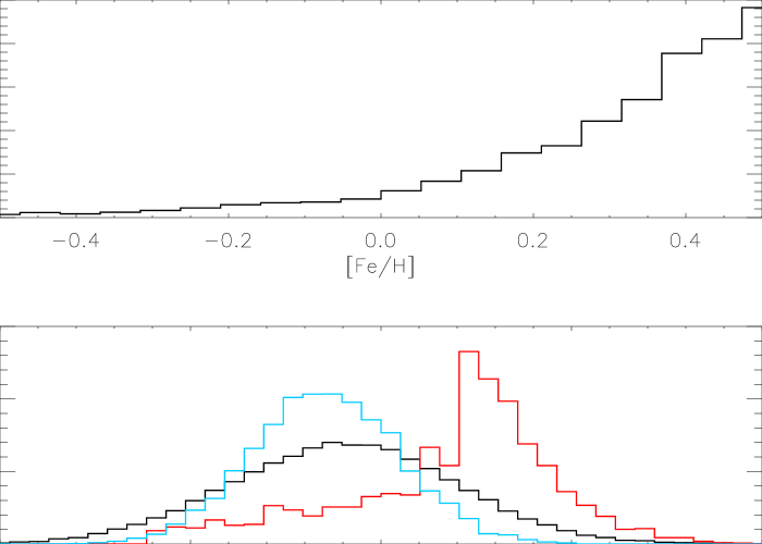
Figure 1: Distribution of stars as a function of their metallicity [Fe/H]. Upper panel: Fraction of stars with planets as a function of their metallicity, as obtained from radial velocity surveys (Santos et al. 2004; Fischer & Valenti 2005). Bottom panel: Normalized distribution of stellar metallicities assumed in Paper I (blue) and in this work (black). The resulting [Fe/H] distribution of planet-hosting stars is also shown in red.

2.4 Statistical evaluation of the performances of the model

As shown in detail in the appendix (see online version), the model is evaluated using univariate, two-dimensional and multivariate statistical tests. Specifically, we show that the parameters for the simulated and observed planets have globally the same mean and standard deviation and that both Student-t tests and Kolmogorov-Smirnov tests indicate that the two populations are statistically indistinguishable. However, while these univariate tests provide preliminary tests of the quality of the data, they are not sufficient because of the multiple correlations between parameters of the problem.

Table 3: Pearson correlations between planetary and stellar characteristics. Significant correlations ($\geq 0.5$) are boldfaced.

	$Y^{\star}$	$\theta$	${\rm[Fe/H]}$	$T_{\rm eff}$	$R_{\star}$	$M_{\star}$	$T_{eq}$	$P$	$R_{p}$	$M_{p}$
$\theta$	$-0.0046$
${\rm[Fe/H]}$	$0.0048$	$0.0560$
$T_{\rm eff}$	$-0.0013$	$-0.1300$	$-0.0227$
$R_{\star}$	$0.0006$	$0.1240$	$-0.0283$	$\mathbf{0.8103}$
$M_{\star}$	$0.0003$	$-0.1301$	$-0.0237$	$\mathbf{0.9359}$	$\mathbf{0.8761}$
$T_{eq}$	$0.0006$	$-0.1411$	$-0.0013$	$\mathbf{0.7338}$	$\mathbf{0.7605}$	$\mathbf{0.7380}$
$P$	$-0.0029$	$0.4184$	$0.0068$	$-0.0304$	$-0.0280$	$-0.0303$	$-0.3990$
$R_{p}$	$0.0015$	$-0.3038$	$\mathbf{-0.5129}$	$\mathbf{0.4833}$	$\mathbf{0.5203}$	$\mathbf{0.5030}$	$\mathbf{0.5191}$	$-0.1931$
$M_{p}$	$-0.0046$	$\mathbf{0.6560}$	$0.0676$	$-0.0317$	$-0.0318$	$-0.0324$	$-0.0476$	$-0.3250$	$-0.1457$
$\star$: variable $Y$ has value 1 if the planet is observed, 0 if it is simulated.

Table 3 presents the Pearson correlation coefficients between each variable. It shows that the problem indeed possesses multiple, complex correlations. In this table, the variable $Y$ characterizes the ‘reality’ of the planet considered (it is equal to $1$ if the planet of the list is an observed one, and to $0$ if it is a simulated planet). We see that $Y$ is very weakly correlated with parameters of the problem. This indicates that the model is well-behaved, but does not constitute a complete validity test in itself.

Table 4 presents the results of a multivariate test using a so-called logistic regression (see the appendix for more details). This method allows to include simultaneously all planet characteristics as predictors of the probability of being a known transiting planet (hereafter named ‘real’ planets as opposed to simulated ones), thereby controlling for the correlations between variables at once. Based on maximum likelihood estimation method, it provides information on whether a given characteritics is positively (resp. negatively) and significantly (resp. non significantly) related with the fact of being a real planet. Moreover, it computes the probability ${\cal{P}}_{\chi^{2}}$ as a general assessment of the quality of the fit. In our case, a large ${\cal{P}}_{\chi^{2}}$ implies no significant difference between the simulated and real planets. Globally, the general fit of the model shows that simulated planets are not significantly distinct from real planets (${\cal{P}}_{\chi^{2}}=0.765$). This can be compared to a model in which model radii are artificially increased by 10%, for which ${\cal P}_{\chi^{2}}\sim 10^{-4}$ (see appendix)

Table 4: Logistic maximum likelihood estimates: $\hat{\beta}$ is indicative of a correlation with $Y$; “t-stat” is the the distance in standard deviations from no correlation, and ${\cal{P}}$ represents the probability that the model and observations are not significantly different.

Variable	$\hat{\beta}$	t-stat.	${\cal{P}}$
$M_{\star}$	0.467	0.63	0.528
${\rm[Fe/H]}$	0.415	1.39	0.164
$T_{\rm eff}$	-0.517	-0.81	0.417
$R_{\star}$	0.059	0.12	0.901
$P$	-0.235	-0.32	0.746
$M_{p}$	0.329	0.35	0.726
$R_{p}$	0.305	0.90	0.370
$T_{eq}$	-0.296	-0.46	0.648
$\theta$	-0.904	-0.58	0.563
Maximum likelihood estimations
Probability ${\cal{P}}_{\chi^{2}}$= 0.756

Table 4 also presents for each seven independent variables of the problem plus the planet equilibrium temperature $T_{eq}$ and Safronov number $\theta$ how a given variable is correlated with the fact that a planet is “real” (as opposed to being one of the simulated planets in the list). The different statistical parameters presented in this table are defined in the appendix. We only provide here a short description: $\hat{\beta}$ is indicative of a correlation between a given variable and the $Y$ (reality) variable. “t-stat” represent the distance from the mean in terms of standard deviations (student-t test). ${\cal{P}}$ represents the probability that the correlation is significant. The two last parameters are evaluated using bootstrap.

The fact that the parameters $\hat{\beta}$ in table 4 are non-zero indicate that there is a correlation between each parameter and the variable $Y$. However, the t-student test indicates that in every case but one (for [Fe/H]), the values obtained for $\hat{\beta}$ are consistent with $0$ to within one standard-deviation: the agreement between model and observations is good. This is further shown by the high ${\cal{P}}$ values (indicative of consistency between model and observations): The lowest ${\cal{P}}$ value is associated with the stellar metallicty ${\rm[Fe/H]}$, but it is high enough not to show a statistically significant difference between our modeled sample and real observations. However, this characteristic is the one with the largest error bars, and the only one to have missing data (for TrES-3, TrES-4, WASP-2 and CoRoT-Exo-2). We included ${\rm[Fe/H]}$, as it is an important feature of our model, in our multivariate analysis, but the comparison with real planets for this characteristic is to be considered carefully. The quality of the agreement between observed planets characteristics and our model improves to $88.4\%$ if we remove ${\rm[Fe/H]}$ from our logistic maximum likelihood estimates (see the appendix for details and further tests).

2.5 Updated mass-radius diagram

Throughout the article, we will use density maps of the simulated detections and compare them to the observations. These density maps use a resolution disk template to get smooth plots. The size of the resolution template is a function of the number of events present in the diagram. The color levels follow a linear density rule for most diagrams we show. In the case of specific diagrams showing rare long period discoveries (more than 5 days) and large surface gravity or Safronov number, we choose to use a logarithmic color range for density maps to emphasize these rare events. A probability map is established using the model detections sample (50,000 detections obtained by simulating multiple times the number of observations from the OGLE survey). Again, we stress that we limited our model to planets below $0.3M_{\rm Jup}$, both because the question of the composition becomes more important and complex for small planets, and because RV detection biases are also more significant. their distribution is only partially known from RV surveys.

Figure 2 shows the mass-radius diagram density map simulated with CoRoTlux and compared to the known planets. Gaps in the diagram at $\sim 3M_{\rm Jup}$ and $\sim 6-7M_{\rm Jup}$ are due to the small sample of close-in RV planets in these ranges and the fact that our mass distribution is obtained by cloning these observed planet rather than relying on a smooth distribution (see Paper I for a discussion). These gaps should disappear with more discoveries of close-in planets by RV. Otherwise, the model distribution and the known planets are in fairly good agreement, as indicated by the $1.7\sim 1.8\sigma$ distance to the maximum likelihood for this diagram (Table 9). However, the agreement is not as good as one would expect probably because of two planets that possess especially large radii CoRoT-Exo-2b and TrES-4b. The existence of these planets is a problem for evolution models in general that goes beyond the present statistical tests that we propose in this article.

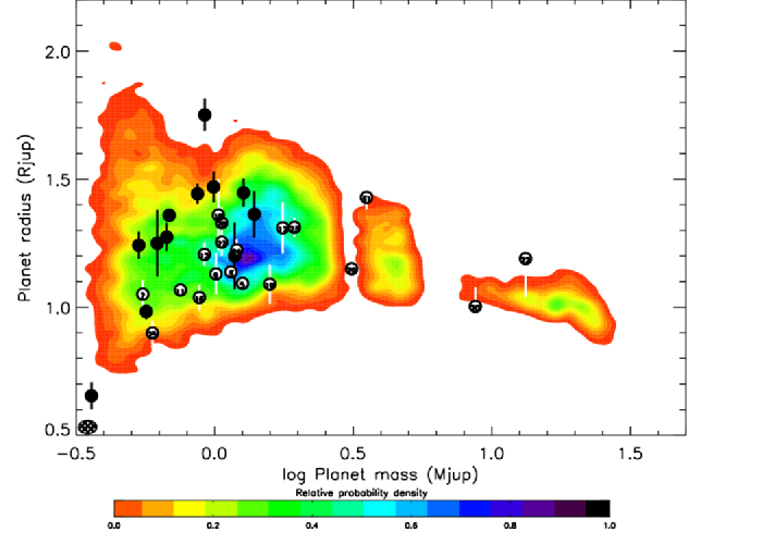
Figure 2: Mass - radius relation for the transiting Pegasids discovered to date (filled circles for planets with low Safronov number $\theta<0.05$, open circles for planets with higher $\theta$ values). The joint probability density map obtained from our simulation is shown as grey contours (or color contours in the electronic version of the article). The resolution disk size used for the contour plot appears in the bottom left part of the picture. At a given (x,y) location the normalized joint probability density is defined as the number of detected planets in the resolution disk centered on (x,y) divided by the maximum number of detected planets in a resolution disk anywhere on the figure.

3 Trends between mass, surface gravity and orbital period

3.1 A correlation between mass and orbital period of Pegasids

Figure 3 compares the known radial-velocity planets to the ones detected in transit. The figure highlights the fact that transit surveys are clearly biased towards detecting short-period planets. However, as shown in Paper I and furthermore reinforced in the present study, the two populations are perfectly compatible provided a limited proportion of very small planets ($P<2$ days) are added.

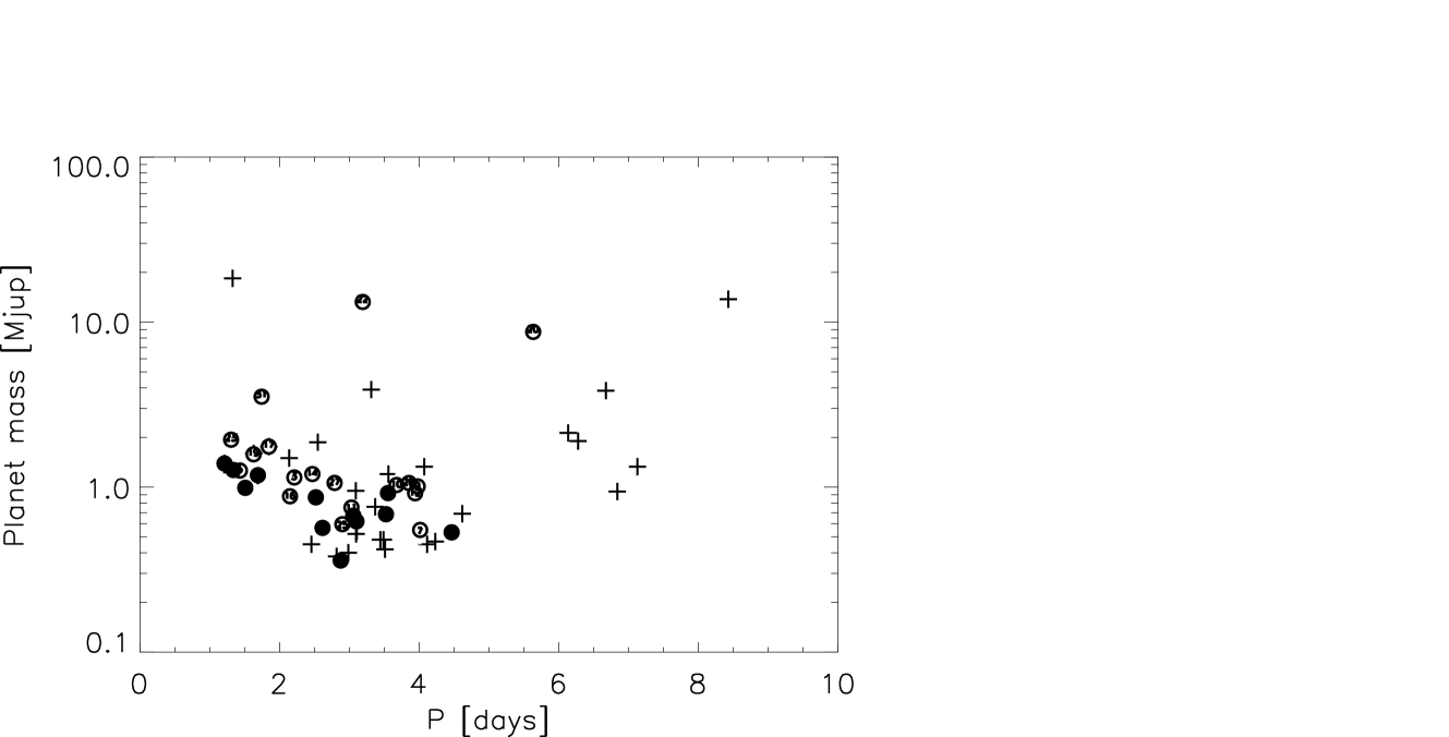
Figure 3: Mass-period distribution of known short-period exoplanets. Crosses correspond to non-transiting planets discovered by radial-velocity surveys. Open and filled circles correspond to transiting planets (with Safronov numbers below and over $0.05$, respectively)

Mazeh et al. (2005) had pointed out the possibility of an intriguing correlation between the masses and periods of the six first known transiting exoplanets. Figure 3 shows that the trend is confirmed with the present sample of planets. This correlation may be due to a migration rate that is inherently dependant upon planetary mass or to other formation mechanisms. It is not the purpose of the present article to analyze this correlation. However, because we use clones of the radial-velocity planets in our model, it is important to stress that this absence of small-mass planets with very short orbital distances can subtend some of the results that will be discussed hereafter.

3.2 A correlation between surface gravity and orbital period of Pegasids ?

The existence of a possible anti-correlation between planetary surface gravity $g=GM_{\rm p}/R_{\rm p}^{2}$ and the orbital period of the nine first transiting planets has been pointed out for some time (Southworth et al. 2007). This correlation still holds (fig. 4) for the Pegasids with periods below 5 days and with jovian masses discovered to date. At the same time, it is important to stress that massive objects (XO-3b, HAT-P-2b and HD17156b) are clear outliers (see fig. 5): Their much larger surface gravity probably implies that they are in a different regime.

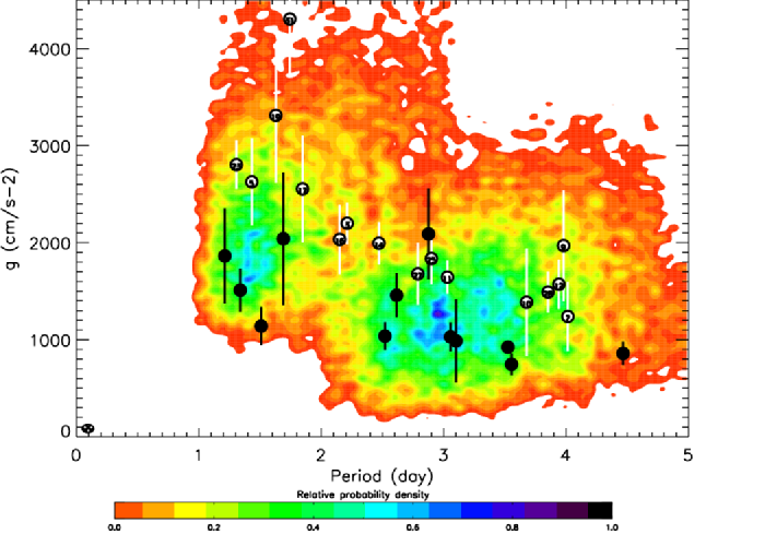
Figure 4: Planetary surface gravity versus orbital period of transiting giant planets discovered to date (circles) compared to a simulated joint probability density map (contours). Symbols and density plot are the same as in fig. 2.

Our model agrees well with the observations (in this $P-g$ diagram real planets are at $0.51$ $\sigma$ from maximum likelihood of the simulated results). We can explain the apparent correlation in Figure 4 as stemming from the existence of two zones with few detectable transiting giant planets:

1. The bottom left part of the diagram where planets are rare, because of a lack of light planets (with low surface gravity) with short periods, as discussed in section 3.1;

2. The upper right part of the diagram (high surface gravity, low planetary radius) where transiting planets are less likely to transit and more difficult to detect.

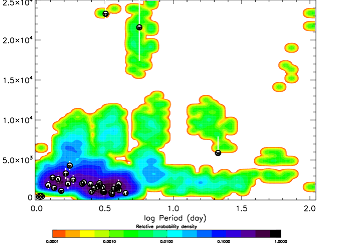
Figure 5: Same figure as Figure 4 with extended surface gravity and period ranges. Note that the scale of the color levels is logarithmic, in order to emphasize the presence of outliers.

Figure 5 shows the same probability density map as in fig. 4 but at a larger scale in period and gravity. The three outliers to the “correlation” appear. These are the large mass planets XO-3b, HAT-P-2b and HD17156b. Given the method chosen to draw the planet population with CoRoTlux, the probability density function that we derive is small, but non-zero around these objects, and also elsewhere in the diagram due to the presence of non-transiting giant planets with appropriate characteristics. Seen at this larger scale, it is clear that the planetary-gravity vs. period relation is much more complex than a simple linear relation.

Globally, figures 4 and 5 indicate that the relation between planet surface gravity and orbital period is not a consequence of a link between the planet composition and its orbital period. Rather, we see it as a consequence of the correlation between planetary mass and orbital period for short period giant planets, which is, as discussed in the previous section, probably linked to mass-dependent migration mechanisms.

4 A correlation between stellar effective temperature and planet radius ?

The range of radius of Pegasids is surprisingly large, especially when one considers the difference in compositions (masses of heavy elements varying from almost 0 to $\sim 100\,\rm M_{\oplus}$) that are required to explain known transiting planets within the same model (Guillot et al. 2006; Guillot 2008). Our underlying planet composition/evolution model is based on the assumption of a correlation of the stellar metallicity with the heavy element content in the planet. We checked that no other variable is responsible for a correlation that would affect this conclusion.

We present the results obtained in the $T_{\rm eff}-R_{\rm p}$ diagram as they are the most interesting: the two variables indeed are positively correlated. Furthermore, given that errors in the stellar parameters are the main sources of uncertainty in the planetary radii determinations, one could suppose that a systematic error in the stellar radius measurement as a function of its effective temperature could be the cause of the variation in the estimated planetary radii. If true, this may alleviate the need for extreme variations in composition. It would cast doubts on the stellar metallicity vs. planetary heavy elements content correlation.

Table 5: Mean planet radius for cool versus hot stars

	Cool stars	Hot stars
	$T_{\rm eff}<5400$ K	$T_{\rm eff}\geq 5400$ K
“Real” planets	$1.072R_{\rm Jup}$	$1.267R_{\rm Jup}$
All simulated planets	$1.058R_{\rm Jup}$	$1.202R_{\rm Jup}$
Detectable simulated planets	$1.074R_{\rm Jup}$	$1.251R_{\rm Jup}$

As shown in Table 5, the mean radius of planets orbiting cool stars ($T_{\rm eff}<5400K$) is $1.072\rm R_{\rm Jup}$ and it is $1.267\rm R_{\rm Jup}$ for planets orbiting hot stars ($T_{\rm eff}\geq 5400K$). Slightly smaller values are obtained in our simulation when considering all transiting planets. However, the values obtained when considering only the detectable transiting planets are in extremely good agreement with the observations.

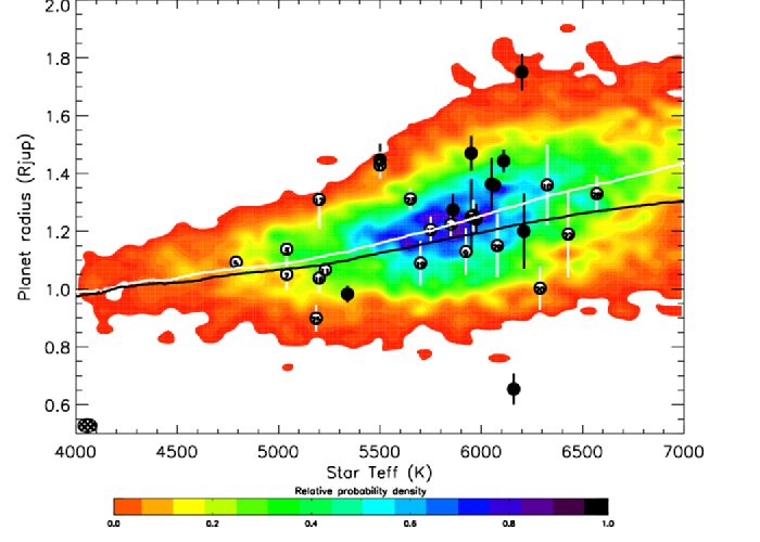
Figure 6: Stellar effective temperature versus planetary radius of transiting giant planets discovered to date (circles) compared to a simulated joint probability density map (contours). The black line is the sliding average of radii in the $[-250K,+250K]$ effective temperature interval for all simulated transiting planets (both below and over the detection threshold). The white line is the same average for the detectable planets in the simulation. The symbols and density map are the same as in fig. 2.

Figure 6 shows in more detail how stellar effective temperature and planetary radius are linked. We interpret the correlation between the two as the combined effect of irradiation (visible with the plotted average radius of all planets with at least one transit event in simulated light curves) and detection bias (visible with the plotted average radius of simulated planets detected):

1. The planets orbiting bright stars are more irradiated. The mean radius of a planet orbiting a warmer star is thus higher at a given period. This effect is taken into account in our planetary evolution model (see Guillot & Showman (2002); Guillot et al. (2006)).

2. The detection of a planet of a given radius is easier for cooler stars since for main sequence stars effective temperature and stellar radius are positively correlated.

We therefore conclude that the effective temperature–planetary radius correlation is a consequence of the physics of the problem rather than the cause of the spread in planetary radii. This implies that another explanation – an important variation of the planetary composition – is needed to account for the observed radii.

As in the mass-radius diagram (fig. 2), there is an outlier at the bottom of figure 6, HD149026b. As discussed previously, this object lies at the boundary of what we could simulate, both in terms of masses and amounts of heavy elements, so that we do not consider this as significant. It is also presently not detectable from a transit survey. Clearly, with more sensitive transit surveys, the presence of low-mass planets with large fraction of heavy elements compared to hydrogen and helium will populate the bottom part of this diagram.

A last secondary outcome of the study of this diagram concerns the possible existence of two groups of planets roughly separated by a $T_{\rm eff}=5400$ K line. We find that the existence of two such groups separated by $\sim 200$ K or more appears serendipitously in our model in 10% of the cases and is therefore absolutely not statistically significant.

5 Two classes of Hot Jupiters, based on their Safronov numbers?

According to Hansen & Barman (2007), the 16 planets discovered at the time of their study show a bimodal distribution in Safronov numbers, half of the sample having Safronov numbers $\theta\sim 0.07$ (“class I”) while the other half is such that $\theta\sim 0.04$ (“class II”). They also point out that the equilibrium temperatures of the two classes of planets differ, the class II planets being on average hotter. This is potentially of great interest because the Safronov number is indicative of the efficiency with which a planet scatters other bodies and therefore this division in two classes, if real, may tell us something about the processes that shaped planetary systems.

5.1 No significant gap between two classes.

Figure 7 shows how the situation has evolved with the new transiting giant planets discovered thus far: Although a few planets have narrowed the gap between the two ensemble of planets, it is still present and located at a Safronov number $\theta\sim 0.05$. The two classes also have mean equilibrium temperatures that differ.

On the other hand, our model naturally predicts a continuous distribution of Safronov numbers. A trend is found in which planets with high equilibrium temperatures tend to have lower Safronov numbers, which is naturally explained by the fact that equilibrium temperature and orbital distance are directly linked (remember that $\theta=(a/R_{\rm p})\,(M_{\rm p}/M_{\star}$)).

We find that our $\theta-T_{\rm eq}$ joint probability density function is representative of the observed population, being at $0.68\sigma$ from the maximum likelihood (see appendix). A K-S test on the Safronov number yields a distance between the observed and simulated distributions of 0.163 and a corresponding probability for a good match of 0.38, a value that should be improved in future models, but that shows that the two ensembles are statistically indistinguishable.

Figure 8 compares the histogram of the distribution of Safronov number for simulated detections with the histogram of real events. Interestingly, although distributions seem different from the $0.05$-scale histogram, with a gap appearing in the $0.05-0.055$ slots, they fit each other while using the $0.1$-scale histogram, more appropriate for this low-number statistics analysis (7 intervals for 31 events).

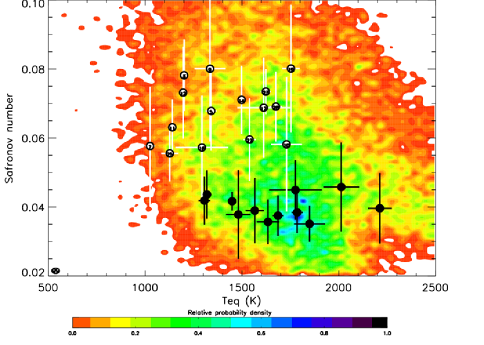
Figure 7: Safronov number versus equilibrium temperature of transiting giant planets discovered to date (circles) compared to a simulated joint probability density map (contours). Open (resp. filled) circles correspond to class I (resp. class II) planets. The symbols and density map are the same as in fig. 2.

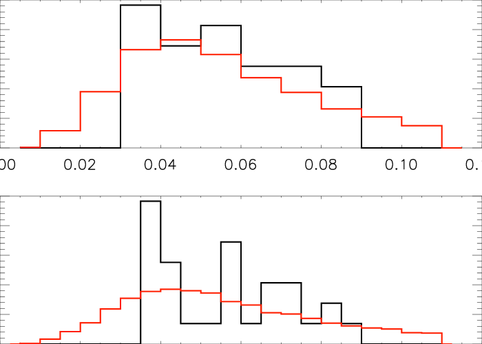
Figure 8: Comparison of the distribution of Safronov number between simulated detections (Red) and real events (Black). Top: histogram with 6 $0.1$-scale columns, Bottom: histogram with 12 $0.05$-scale columns.

Figure 9 shows the probability to obtain a gap of a given size between the Safronov numbers of two potential groups of a random draw. 26 of the known transiting Pegasids have their Safronov number between 0 and 0.1. Setting a minimum number of 5 planets in each of two classes, we look for the largest gap between Safronov numbers of a random draw of 26 simulated Pegasids. For each one of the 10000 Monte-Carlo draws among the model detections sample, we calculate how large is the most important difference between successive Safronov numbers of the 26 random draws. We find that a gap of $0.0102$ between two potential groups is an uncommon event (10 % of the cases, as 4 % of the cases have gaps of this size, and a total of 6 % of the cases have larger gaps), yet it is not exceptionally rare. Considering the 7 planet/star characteristics and their many possible combinations, this level of ”rarity” is not statistically significant.

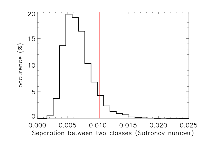
Figure 9: Occurrence of the largest observed separation of Safronov numbers between two ‘groups’ selected in random draws among the model detections sample. The vertical line shows the separation ($0.0102$) between the two classes of planets as inferred from the observational sample.

It is also interesting to consider the few high-Safronov-number planets discovered as in Figure 10. The different gaps in the diagram are due to our mass vs. period carbon copies of RV planets that do not uniformly cover the space of parameters. The desert part in the right edge of the density map is due to the absence of massive planets in the $[3,15]M_{\rm Jup}$ range at close orbit in the RV planets. The simulated detections at both high Safronov number and equilibrium temperature correspond to simulated clones of the planet HD41004b, with its large mass of 18 $M_{\rm Jup}$ and its very close-in period of $1.33$ days.

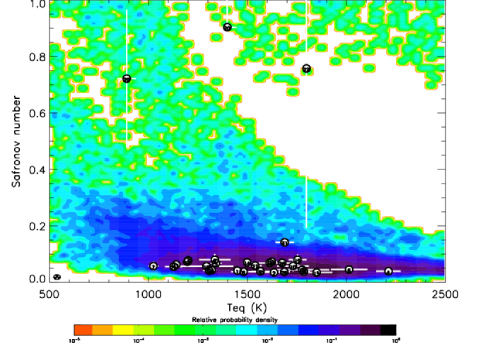
Figure 10: Same as Figure 7 but for a larger range of Safronov numbers. Note that the scale of the color levels is logarithmic, in order to emphasize the presence of outliers.

5.2 No bimodal distribution visible in other diagrams.

When plotted as a function of different stellar (effective temperature, mass, radius) and planetary characteristics (mass, radius, period, equilibrium temperature), the two potential Safronov classes do not differ in a significant way. When plotting our simulated detections as a function of their Safronov number in different diagrams, the two groups formed by cutting our model detections sample with a Safronov number cut-off set at $0.05$ partly overlap each other on most diagrams. Here, we choose to present the planetary mass vs. equilibrium temperature diagram which used to provide a clear separation between the two populations (Hansen & Barman 2007; Torres et al. 2008). We present in fig 11 this diagram as an example of partial overlap of the class I and class II detected planets and probability density maps. Contrary to indications based on a smaller sample of observations, there is no more a clear separation in this diagram between class I and class II planets.

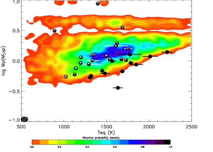
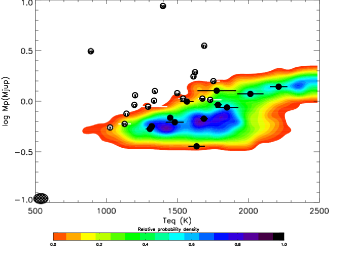
Figure 11: Planetary mass versus equilibrium temperature of transiting giant planets discovered to date (circles) compared to a simulated joint probability density map (contours). Top panel: The density map accounts only for simulated planets with a Safronov number $\theta>0.05$ (class I planets). Bottom panel: The density map corresponds only to planets with $\theta<0.05$ (class II planets). The symbols and density maps are the same as in fig. 2.

5.3 No correlation between metallicity and Safronov number/class.

Torres et al. (2008) showed that a significant difference could be observed between the metallicity distributions of the two Safronov classes. The high-Safronov number class (class I, $\theta>0.05$) had its host star metallicity centered on $0.0$, and the low-Safronov number class (class II) was centered on $0.2$. They pointed out that the Safronov numbers for Class I planets show a decreasing trend with metallicity.

The two recent discoveries of CoRoT-Exo-1-b ($\rm{\rm[Fe/H]}=-0.4$ and $\theta=0.038$) and OGLE TR182-b ($\rm{\rm[Fe/H]}=0.37$ and $\theta=0.08$) tend to contradict this argument. Considering the 31 known giant planets, the mean metallicity of stars hosting class I planets is now $\rm{\rm[Fe/H]}=0.6$, and it is $1.6$ for class II planets. Figure 12 shows that although the metallicity vs. Safronov number distribution of detections we simulate is a likely result ($0.63\sigma$ from maximum likelihood), the potential anticorrelation between $\theta$ and host star [Fe/H] (pointed out by Torres et al. (2008)) for class I planets is not present in our simulation, which shows a continouous density map.

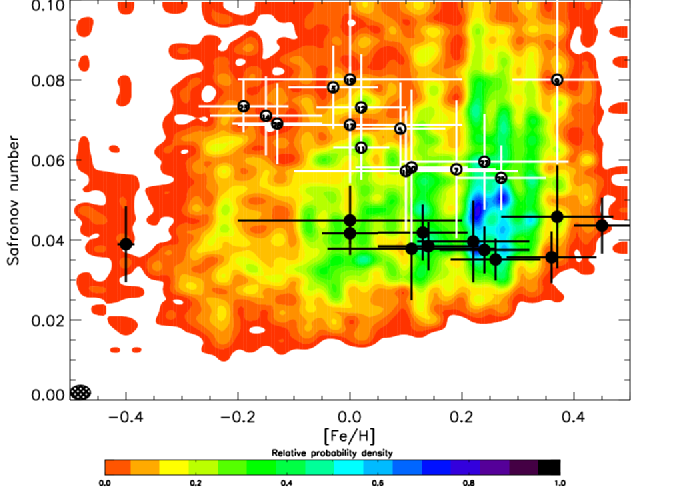
Figure 12: Safronov number of transiting planets as a function of their host star metallicity. The density map with linear contours comes from the model detections sample. Open and filled circles are respectively class I planets [with Safronov number over $0.05$] and class II planets [with Safronov number below $0.05$] Symbols and density plot are the same as in fig. 2.

5.4 No significant gap between two Safronov number classes.

Our study has shown us that a separation between two groups of planets linked to their Safronov number is unlikely for at least two reasons:

1. The separation between the two groups is marginal. It only appears in the Safronov number histogram if the resolution of the histogram is high in comparison to the number of events sampled. The separation of $\sim 0.01$ between two possible Safronov classes has a non-negligible $10\%$ probability to occur serendipitously in our distribution which is otherwise continuous. Considering the relatively numerous parameters (4 for the star, 3 linked with the planet) and their combinations, such a division in two groups appears quite likely to occur fortuitously for one such parameter.

2. The separation between the two classes is not present on any figures other than the ones involving the Safronov number itself. This includes also the separation in metallicity vs. $\theta$ which is not statistically significant, especially given recent discoveries of CoRoT-Exo-1b and OGLE-TR-182b .

On the other hand, we cannot formally rule out the existence of these two groups of planets. We hence eagerly await other observations of transiting planets for further tests.

6 Conclusions

We have presented a coherent model of a population of stars and planets that matches within statistical errors the observations of transiting planets performed thus far. Thanks to new observations, we have improved on our previous model (Paper I). In particular, we now show that with slightly improved assumptions about the metallicity of stars in the solar neighborhood, the metallicity of stars with transiting giant planets can be explained without assuming any bias in period vs. metallicity.

In order to validate our model, we have used a series of univariate, bivariate and multivariate statistical tests. As the sample of radial-velocimetry planets and of transiting planets grow, we envision that with these tools we will be able to much better characterize the planet population in our Galaxy and its dependence with star population, and also test models of planet formation and evolution.

With today’s sample of transiting planets, our model provides a very good match with the observations, both when considering planetary and stellar parameters one by one or globally. Our analysis has revealed that the parameters for the modeled planets are presently statistically indistinguishable from the observations, although there may be room for improvement of the model. It should be noted that our underlying assumptions for the compositions and evolution of planets and for the stellar populations are relatively simple. With a larger statistical sample, tests of these assumptions will be possible and will bring important constraints on the planet-star distribution in our galactic neighborhood. The CoRoT mission is expected to be very important in that respect, especially given the careful determination of the characteristics of the stellar population that is being monitored.

Using this method, we have been able to analyze and explain the different correlations observed between transiting planets characteristics:

1. Mass vs. period: One of the first correlations observed among the planet/star characteristics was the mass vs. period of close-in RV planets (Mazeh et al. 2005). Although our model does not explain it, we confirm with a sample that is now 4 times larger than at the time of the publication that there is a lack of low-mass planets ($M_{p}$ $<1\rm M_{\rm Jup}$) on very short periods ($P<2$ days).

2. Surface gravity vs. period: There is an inverse correlation between the surface gravity and period of transiting planets. We show that this correlation is caused by the above mass vs. period effect, and by a lower detection probability for planets with longer periods and higher surface gravities.

3. Radius vs. stellar effective temperature: Planets around stars with larger effective temperatures tend to have larger sizes. This is naturally explained by a combination of slower contraction due to the larger irradiation and by the increased difficulty in finding planets around hotter, larger stars.

4. Safronov number: Hansen & Barman (2007); Torres et al. (2008) have identified a separation between two classes of planets, based on their Safrononov number, and visible in different diagrams ($\theta$ vs. $T_{eq}$ and vs. ${\rm[Fe/H]}$, $M_{p}$ vs. $T_{eq}$). With recent discoveries, this separation is still present in the Safronov number distribution, but not anymore in other diagrams. On the other hand, our simulation predicts distributions that are continuous, in particular in terms of Safronov number. With this continuous distribution, we show that a random draw of 30 simulated planets produces two spurious groups separated in Safronov number by a distance equal to or larger than the observations in 30% of the cases. The separation is not visible and significant between the two classes in any other diagram we plotted. Therefore, we conclude that the separation in two classes is not statistically significant but is to be checked again with a larger sample of observed planets. Interestingly, if on the contrary two classes of Safronov numbers were found to exist we would have to revise our model for the composition of planets.

In the next few years, precise analyses of surveys with well-defined stellar fields and high yields (like CoRoT and Kepler) will allow to precisely test different formation theories and to link planetary and stellar characteristics. It should also allow precising the laws behind the occurrence of planets and their orbital and physical parameters. Up to now, we have focused on giant planets, but with larger statistical samples, we hope to be able to extend these kind of studies to planets of smaller masses which will be intrinsically more complex because of a larger variety in their compositions (rocks, ices, gases). Altogether, this stresses the need for a continuation of radial-velocity and photometric surveys for, and follow-up observations of, new transiting planets to greatly increase the sample of known planets and obtain accurate stellar and planetary parameters. The goal is of importance: to better understand what our galactic neighborhood is made of.

Online data

Appendix: Statistical evaluation of the model

6.1 Univariate tests on individual planet characteristics

In this section, we detail the statistical method and tests that have been used to validate the model. We first perform basic tests of our model with simulations repeating multiple timesthe number of observations of the OGLE survey in order to get $50,000$ detections. This number was chosen as a compromise between statistical significance and computation time. Table 6 compares the mean values and standard variations in the observations and in the simulations. The closeness of the values obtained for the two populations is an indication that our approach provides a reasonably good fit to the real stellar and planetary populations, and to the real planet compositions and evolutions.

Table 6: Mean values and standard deviations for the system parameters for the observed transiting planets and our simulated detections.

real planets
	$M_{p}$	$R_{p}$	$P$	$T_{eq}$	$M_{\star}$	$R_{\star}$	$T_{\rm eff}$	${\rm[Fe/H]}$	$\theta$
mean	1.834	1.235	3.387	1510	1.094	1.164	5764	0.087	0.148
$\sigma$	2.645	0.178	3.540	300.2	0.186	0.304	464	0.187	0.270
simulated detections
	$M_{p}$	$R_{p}$	$P$	$T_{eq}$	$M_{\star}$	$R_{\star}$	$T_{\rm eff}$	${\rm[Fe/H]}$	$\theta$
mean	1.655	1.248	3.217	1564	1.073	1.167	5813	0.07805	0.129
$\sigma$	2.401	0.186	2.897	411.0	0.195	0.324	599	0.217	0.270

However, we do require more advanced statistical tests. First, we use the so-called Student’s t-test to formally compare the mean values of all characteristics for both types of planets. The intuition is that, should the model yield simulated planets of attributes similar to real planets, the average values of these attributes should not be significantly different from one another. In other words, the so-called null hypothesis $H_{0}$ is that the difference of their mean is zero. Posing $H_{0}$: $\mu^{r}-\mu^{s}=0$ where superscripts $r$ and $s$ denote real and simulated planets respectively, and the alternative hypothesis $H_{a}$ being the complement $H_{a}$: $\mu^{r}-\mu^{s}\neq 0$, we compute the $t$ statistics using the first and second moments of the distribution of each planet characteristics as follows:

$$t=\frac{{\left({\mu_{x}^{r}-\mu_{x}^{s}}\right)}}{{\frac{{s_{p}}}{{\sqrt{n_{r}+n_{s}}}}}},$$ (2)

where $x$ is each of the planet characteristics, $n$ is the size of each sample, and $s_{p}$ is the square root of the pooled variance accounting for the sizes of the two population samples. The statistics follows a $t$ distribution, from which one can easily derive the two-tailed critical probability that the two samples come from one unique population of planets, i.e. $H_{0}$ cannot be rejected. The results are displayed in Table 7 (Note that $\theta$ is the Safronov number; other parameters have their usual meaning). In all cases, the probabilities are larger than 40%, implying that there is no significant difference in the mean characteristics of both types of planets. In other words, the two samples exhibit similar central tendencies.

Table 7: Test of equality of means. Student’s $t$ value and critical probabilities $p$ that individual parameters for both real and simulated planets have the same sample mean.

parameter	$t$	$p$
$M_{\star}$	-0.277	0.782
${\rm[Fe/H]}$	-0.392	0.695
$T_{\rm eff}$	0.707	0.480
$R_{\star}$	0.331	0.741
$P$	-0.276	0.783
$M_{p}$	-0.570	0.569
$R_{p}$	0.642	0.521
$T_{eq}$	0.834	0.405
$\theta$	-0.585	0.559

Next, we perform the Kolmogorov-Smirnov test to allow for a more global assessment of the compatibility of the two populations. This test has the advantage of being non-parametric, making no assumption about the distribution of data. This is particularly important since the number of real planets remains small, which may alter the normality of the distribution. Moreover, the Kolmogorov-Smirnov comparison tests the stochastic dominance of the entire distributions of real planets over simulated planets. To do so, it computes the largest absolute deviations $D$ between $F_{r}(x)$, the empirical cumulative distribution function of characteristics $x$ for real planets, and $F_{s}(x)$ the cumulative distribution function of characteristics $x$ for simulated planets, over the range of values of $x$: $D=\mathop{\max}\limits_{x}\left\{{\left|{F_{real}\left(x\right)-F_{sim}\left(x\right)}\right|}\right\}$. If the calculated $D$-statistic is greater than the critical $D^{*}$-statistic (provided by the Kolmogorov-Smirnov table –for 31 observations $D^{*}=0.19$ for a 80% confidence level and $D^{*}=0.24$ for a 95% confidence level–), then one must reject the null hypothesis that the two distributions are similar, $H_{0}:|F_{r}(x)-F_{s}(x)|<D^{*}$, and accept $H_{a}:|F_{r}(x)-F_{s}(x)|\geq D^{*}$. Table 8 shows the result of the test. The first column provides the D-Statistics, and the second column gives the probability that the two samples have the same distribution.

Table 8: Kolmogorov-Smirnov tests. $D$-statistics and critical probabilities that individual parameters for both real and simulated planets have the same distribution.

parameter	$D$	$p$
$M_{\star}$	0.154	0.492
${\rm[Fe/H]}$	0.161	0.438
$T_{\rm eff}$	0.135	0.662
$R_{\star}$	0.141	0.612
$P$	0.145	0.572
$M_{p}$	0.173	0.347
$R_{p}$	0.126	0.745
$T_{eq}$	0.180	0.303
$\theta$	0.163	0.381

Again, we find a good match between the model and observed samples: the parameters that have the least satisfactory fits are the planet’s equilibrium temperature and the planet mass respectively. These values are interpreted as being due to imperfections in the assumed star and planet populations. It is important to stress that although the extrasolar planets’ main characteristics (period, mass) are well-defined by the radial-velocity surveys, the subset of transiting planets is highly biased towards short periods and corresponds to a relatively small sample in the known radial-velocity planet population. This explains why the probability that the planetary mass is drawn from the same distribution in the model and in the observations is relatively low, which may otherwise seem surprising given that the planet mass distribution would be expected to be relatively well defined by the radial-velocity measurements.

6.2 Tests in two-dimensions

Tests of the adequation of observations and models in two dimensions,i.e. when considering one parameter as compared to another one can be performed using the method of maximum likelihood as described in Paper I. Table 9 provides values of the standard deviations from maximum likelihood for important combinations of parameters. The second column is a comparison using all planets discovered by transit surveys, and the third column using all known transiting planets (including those discovered by radial velocity).

Table 9: Standard deviations from maximum likelihood of the model and observed transiting planet populations

parameter	planets from	all planets
	transit surveys
$M_{\star}$ vs. P	1.19 $\sigma$	1.25 $\sigma$
$M_{\star}$ vs. P	1.48 $\sigma$	1.62 $\sigma$
$R_{p}$ vs. $M_{p}$	1.70 $\sigma$	1.82 $\sigma$
P vs. ${\rm[Fe/H]}$	1.09 $\sigma$	1.09 $\sigma$
$R_{p}$ vs. ${\rm[Fe/H]}$	1.61 $\sigma$	1.71 $\sigma$
g vs. P	0.61 $\sigma$	0.51 $\sigma$
$\theta$ vs. $T_{\rm eff}$	0.68 $\sigma$	0.63 $\sigma$
$R_{p}$ vs. $T_{\rm eff}$	1.22 $\sigma$	1.45 $\sigma$

The results are generally good, with deviations not exceeding $1.82\sigma$. They are also very similar when considering all planets or only the subset discovered by photometric surveys. This shows that the radial-velocity and photometric planet characteristics are quite similar. The mass vs. radius relation shows the highest deviation, as a few planets are outliers of our planetary evolution model.

6.3 Multivariate assessment of the performance of the model

6.3.1 Principle

Tests such as the student-t statistics and the Kolmogorov-Smirnov test are important to determine the adequation of given parameters, but they do not provide a multivariate assessment of the model. In order to assess globally the viability of our model we proceed as follows: We generate a list including 50,000 “simulated” planets and the 31 “observed” giant planets from Table 1. This number is necessary to get an accurate multi-variate analysis (see paragraph 6.3.2). A dummy variable $Y$ is generated with value $1$ if the planet is observed, $0$ if the planet is simulated.

In order to test dependencies between parameters, we have presented in table 3 (§ 2.4) the Pearson correlation coefficients between each variable including $Y$. A first look at the table shows that the method rightfully retrieves the important physical correlation without any a priori information concerning the links that exist between the different parameters. For example, the stellar effective temperature $T_{\rm eff}$ is positively correlated to the stellar mass $M_{\star}$, and radius $R_{\star}$. It is also naturally positively correlated to the planet’s equilibrium temperature $T_{\rm eq}$, and to the planet’s radius $R_{\rm p}$ simply because evolution models predict planetary radii that are larger for larger values of the irradiation, all parameters being equal. Interestingly, it can be seen that although the Safronov number is by definition correlated to the planetary mass, radius, orbital period and star mass (see eq. 1), the largest correlation parameters for $\theta$ in absolute value are those related to $M_{p}$ and $P$ (as the range of these parameters both vary by more than one decade, while $M_{\star}$ and $R_{p}$ only vary by a factor $2$). Also, we observe that the star metallicity is only correlated to the planet radius. This is a consequence of our assumption that a planet’s heavy element content is directly proportional to the star’s [Fe/H], and of the fact that planets with more heavy elements are smaller, all other parameters being equal. The planet’s radius is itself correlated negatively with [Fe/H] and positively with $T_{\rm eq}$, $M_{\star}$,$R_{\star}$ and $T_{\rm eff}$. Table 3 also shows the correlations with the “reality” parameter. Of course, a satisfactory model is one in which there is no correlation between this reality parameter and other physical parameters of the model. In our case, the corresponding correlation coefficients are always small and indicate a good match between the two populations.

Obviously the unconditional probability that a given planet is real is $\Pr(Y=1)=31/50031\simeq.00062$. Now we wish to know whether this probability is sensitive to any of the planet characteristics, controlling for all planet characteristics at once. Hence we model the probability that a given planet is ”real” using the logistic cumulative density function as follows:

$$\Pr(Y=1|{\mathbf{X_{i}}})=\frac{{e^{{\mathbf{X_{i}{b}}}}}}{{1+e^{{\mathbf{X_{i}{b}}}}}}$$ (4)

where $\mathbf{X_{i}}$ is the vector of explanatory variables (i.e. planet characteristics) for the planet $i$ (real or simulated), and $\mathbf{{b}}$ is the vector of parameter to be estimated, and $\mathbf{X_{i}{b}}\equiv b_{0}+\sum_{j}X_{ij}b_{j}$, and $b_{0}$ is a constant. There are $n$ events to be considered ($i=1..n$) and $m$ explanatory variables ($j=1..m$).

Importantly, an ordinary least square estimator shall not be used in this framework, due to the binary nature of the dependent variables. (Departures from normality and predictions outside the range $[0;1]$ are the quintessential motivations). Instead, Equation 4 can be estimated using maximum likelihood methods. The so-called logit specification (Greene 2000) fits the parameter estimates $\mathbf{{b}}$ so as to maximize the log likelihood function :

$$\log L({\mathbf{Y}}|{\mathbf{X,{b}}})=\sum\limits_{i=1}^{n}{y_{i}\ {{\mathbf{X_{i}{b}}}}}-\sum\limits_{i=1}^{n}{\log\left[{1+e^{{\mathbf{X_{i}{b}}}}}\right]}.$$ (5)

The $\log L$ function is then maximized choosing $\mathbf{\hat{b}}$ such that ${\partial\log L(y_{i},{\mathbf{X_{i},\hat{b}}})}/{\partial\mathbf{\hat{b}}}=0$, using a Newton-Raphson algorithm. The closer the coefficients $\hat{b}_{1},\hat{b}_{2},..,\hat{b}_{m}$ are to $0$, the closer the model is to the observations. Conversely, a coefficient that is significantly different from zero tells us that there is a correlation between this coefficient and the probability for a planet to be “real”, i.e. the model is not a good match to the observations.

Two features of logistic regression using maximum likelihood estimators are worth to be mentioned. First, the value added of the exercise is that the multivariate approach allows us to hold all other planet characteristics constant, extending the bivariate correlations to the multivariate case. In other words, we control for all planet characteristics at once. Second, one can test whether a given parameter estimate is equal to 0 with the usual null hypothesis $H_{0}$: ${b}=0$ versus $H_{a}$: ${b}\neq 0$. The variance of the estimator is used to derive the standard error of the parameter estimate. Using equation 6, dividing for each variable $\hat{{b}}_{j}$ by the standard error ${\rm s.e.}(\hat{{b}}_{j})$ yields the t-statistics and allows us to test $H_{0}$. We note ${\cal P}_{j}$ the probability that a higher value of $t$ would occur by chance . This probability is evaluated for each explanatory variable $j$. Should our model perform well, we would expect the $t$ value of each parameter estimate to be null, and the corresponding probability ${\cal P}_{j}$ to be close to one. This would imply no significant association between a single planet characteristics and the event of being a ”real” planet.

Last but not least, the global probability that the model and observations are compatible can be estimated. To do so, we compute the log likelihood obtained when $b_{j}=0$ for $j=1..m$, where $m$ is the number of variables. Following eq. (6):

$$\log L({\mathbf{Y}}|1,b_{0})=\sum\limits_{i=1}^{n}{y_{i}b_{0}}-\sum\limits_{i=1}^{n}{\log\left[{1+e^{b_{0}}}\right]}.$$ (6)

The maximum of this quantity is $\log L_{0}=n_{0}\log(n_{0}/n)+n_{1}\log(n_{1}/n)$, where $n_{0}$ is the number of cases in which $y=0$ and $n_{1}$ is the number of observations with $y=1$. $L_{0}$ is thus the maximum likelihood obtained for a model which is in perfect agreement with the observations (no explanatory variable is correlated to the probability of being real). Now, it can be shown that the likelihood statistic ratio

$$c_{\rm LL}=2(\log L_{1}-\log L_{0})$$ (7)

follows a $\chi^{2}$ distribution for a number of degrees of freedom $m$ when the null hypothesis is true (Aldrich & Nelson (1984)). The probability that a sum of $m$ normally distributed random variables with mean $0$ and variance $1$ is larger than a value $c_{\rm LL}$ is:

$${\cal P}_{\chi^{2}}=P(m/2,c_{\rm LL}/2),$$ (8)

where $P(k,z)$ is the regularized Gamma function (e.g. Abramowitz & Stegun (1964)). ${\cal{P}}_{\chi^{2}}$ is thus the probability that the model planets and the observed planets are drawn from the same distribution.

6.3.2 Determination of the number of model planets required

A problem that arose in the course of the present work was to evaluate the number of model planets that were needed for the logit evaluation. It is often estimated that about 10 times more model points than observations are sufficient for a good tests. We found that this relatively small number of points indeed leads to a valid identification of the explanatory variables that are problematic, i.e. those for which the $\hat{b}$ coefficient is significantly different from $0$ (if any). However, the evaluation of the global $\chi^{2}$ probability was then found to show considerable statistical variability, probably given the relatively large number of explanatory variables used for the study.

In order to test how the probability ${\cal{P}}_{\chi^{2}}$ depends on the size n of the sample to be analyzed, we first generated a very large list of $N_{0}$ simulated planets with CoRoTlux. We generated by Monte-Carlo a smaller subset of $n_{0}\leq N_{0}$ simulated planets that was augmented of the $n_{1}=31$ observed planets and computed ${\cal{P}}_{\chi^{2}}$ using the logit procedure. This exercise was performed 1000 times, and the results are shown in fig. 13. The resulting ${\cal{P}}_{\chi^{2}}$ is found to be very variable for a sample smaller than $\sim 20,000$ planets. As a consequence, we chose to present tests performed for $n_{0}=50,000$ model planets.

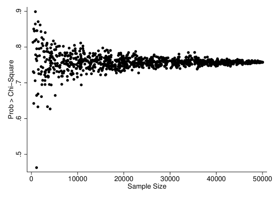
Figure 13: Values of the $\chi^{2}$ probability, ${\cal{P}}_{\chi^{2}}$ (see text) obtained after a logit analysis as a function of the size of the sample of model planets $n_{0}$.

6.3.3 Analysis of two CoRoTlux samples

Table 4 (see § 2.4) reports the parameter estimates for each of the planet/star characteristics. We start by assessing the general quality of the logistic regression by performing the chi-square test. If the vector of planet characteristics brings no or little information as to which type of planets a given observation belongs to, we would expect the logistic regression to perform badly. In technical terms, we would expect the conditional probability $\Pr(Y=1|{\mathbf{X}})$ to be equal to the unconditional probability $\Pr(Y=1)$. The $\chi^{2}$ test described above is used to evaluate the significance of the model.

We performed several tests: the first column of results in table 10 shows the result of a logit analysis with the whole series of 9 explanatory variables. Globally, the model behaves well, with a likelihood statistic ratio $c_{\rm LL}=5.8$ and a $\chi^{2}$ distribution for 9 degrees of freedom yielding a probability ${\cal{P}}_{\chi^{2}}=0.758$. When examining individual variables, we find that the lowest probability derived from the Student test is that on [Fe/H]: ${\cal{P}}_{\rm{\rm[Fe/H]}}=0.164$, implying that the stellar metallicity is not well reproduced. As discussed previously, this is due to the fact that several planets of the observed list have no or very poorly constrained determination of the stellar [Fe/H], and that a default value of $0$ was then used.

The other columns in table 10 show the result of the logit analysis when removing one variable (i.e. with only 8 explanatory variables). In agreement with the above analysis, the highest global probability ${\cal{P}}_{\chi^{2}}$ is obtained for the model without the [Fe/H] variable. When removing other variables, the results are very homogeneous, indicating that although the model can certainly be improved, there is no readily identified problem except that on [Fe/H]. (We hope that future observations will allow for better constraints on these stars’ metallicities).

In order to further test the method, we show in table 11 the results of an analysis in which the model radii where artificially augmented by 10%. The corresponding probabilities are significantly lower: we find that the model can explain the observations by chance only in less than 1/10,000. The probabilities for each variable are affected as well so that it is impossible to identify the culprit for the bad fit with the 9 variables. However, when removing $R_{\rm p}$ from the analysis sample, the fit becomes significantly better. (Note that the results for that column are slightly different than those for the same column in table 10 because of the dependance of $\theta$ with $R_{\rm p}$.)

Table 10: Result of the logit analysis for the fiducial model with 50,000 model planets and 31 observations.

		All variables	Missing variable
			[Fe/H]	$T_{eff}$	$R_{\star}$	$M_{\star}$	$P$	$R_{p}$	$M_{p}$	$\theta$	$T_{eq}$
[Fe/H]	${\hat{b}}_{{\rm[Fe/H]}}$	0.415		0.435	0.413	0.430	0.421	0.229	0.385	0.371	0.369
	${\cal P}_{{\rm[Fe/H]}}$	[0.164]		[0.148]	[0.164]	[0.150]	[0.157]	[0.242]	[0.177]	[0.196]	[0.182]
$T_{eff}$	${\hat{b}}_{T_{\rm eff}}$	-0.517	-0.579		-0.541	-0.191	-0.569	-0.563	-0.541	-0.537	-0.618
	${\cal P}_{T_{\rm eff}}$	[0.417]	[0.366]		[0.372]	[0.601]	[0.355]	[0.378]	[0.391]	[0.395]	[0.298]
$R_{\star}$	${\hat{b}}_{R_{\rm{\star}}}$	0.059	0.046	0.190		0.212	-0.009	0.061	0.027	0.023	-0.063
	${\cal P}_{R_{\rm{\star}}}$	[0.901]	[0.924]	[0.681]		[0.609]	[0.984]	[0.898]	[0.953]	[0.961]	[0.871]
$M_{\star}$	${\hat{b}}_{M_{\rm{\star}}}$	0.467	0.541	-0.001	0.511		0.472	0.524	0.483	0.486	0.497
	${\cal P}_{M_{\rm{\star}}}$	[0.528]	[0.468]	[0.998]	[0.433]		[0.523]	[0.481]	[0.512]	[0.508]	[0.499]
$P$	${\hat{b}}_{P}$	-0.236	-0.288	-0.425	-0.199	-0.250		-0.281	-0.269	-0.356	-0.070
	${\cal P}_{P}$	[0.746]	[0.698]	[0.605]	[0.754]	[0.737]		[0.706]	[0.708]	[0.618]	[0.883]
$R_{p}$	${\hat{b}}_{R_{\rm p}}$	0.305	-0.069	0.331	0.305	0.328	0.316		0.261	0.246	0.241
	${\cal P}_{R_{\rm p}}$	[0.370]	[0.778]	[0.332]	[0.370]	[0.336]	[0.352]		[0.416]	[0.456]	[0.443]
$M_{p}$	${\hat{b}}_{M_{\rm p}}$	0.329	-0.032	0.432	0.306	0.379	0.386	0.055		-0.229	0.118
	${\cal P}_{M_{\rm p}}$	[0.726]	[0.968]	[0.656]	[0.737]	[0.693]	[0.674]	[0.947]		[0.474]	[0.876]
$\theta$	${\hat{b}}_{\theta}$	-0.904	-0.496	-1.005	-0.879	-0.971	-1.049	-0.625	-0.422		-0.653
	${\cal P}_{\theta}$	[0.563]	[0.706]	[0.540]	[0.567]	[0.548]	[0.497]	[0.658]	[0.410]		[0.620]
$T_{eq}$	${\hat{b}}_{T_{\rm eq}}$	-0.296	-0.023	-0.520	-0.250	-0.339	-0.169	-0.089	-0.186	-0.150
	${\cal P}_{T_{\rm eq}}$	[0.648]	[0.970]	[0.414]	[0.635]	[0.605]	[0.744]	[0.882]	[0.742]	[0.801]
overall assessment of the fit
Log likelihood		-257.059	-258.123	-257.410	-257.066	-257.275	-257.129	-257.439	-257.126	-257.316	-257.171
$c_{\rm LL}$		5.821	3.692	5.119	5.805	5.389	5.681	5.060	5.687	5.307	5.597
${\cal{P}}_{\chi^{2}}$		0.758	0.884	0.745	0.669	0.715	0.683	0.751	0.682	0.724	0.692

Table 11: Result of the logit analysis for the altered model ($R_{\rm p}$ increased by 10%) with 50,000 model planets and 31 observations.

		All variables	Missing variable
			${\rm[Fe/H]}$	$T_{eff}$	$R_{\star}$	$M_{\star}$	$P$	$R_{p}$	$M_{p}$	$\theta$	$T_{eq}$
[Fe/H]	${\hat{b}}_{{\rm[Fe/H]}}$	-0.738		-0.740	-0.737	-0.737	-0.733	0.224	-0.607	-0.728	-0.664
	${\cal P}_{{\rm[Fe/H]}}$	[0.002]		[0.002]	[0.002]	[0.002]	[0.002]	[0.251]	[0.009]	[0.002]	[0.005]
$T_{\rm eff}$	${\hat{b}}_{T_{\rm eff}}$	-0.729	-0.713		-0.742	-0.255	-0.819	-0.573	-0.545	-0.739	-0.308
	${\cal P}_{T_{\rm eff}}$	[0.260]	[0.268]		[0.231]	[0.483]	[0.192]	[0.366]	[0.404]	[0.256]	[0.618]
$R_{\star}$	${\hat{b}}_{R_{\rm{\star}}}$	0.032	0.013	0.197		0.247	-0.091	0.032	0.237	0.018	0.558
	${\cal P}_{R_{\rm{\star}}}$	[0.945]	[0.978]	[0.661]		[0.540]	[0.828]	[0.945]	[0.620]	[0.970]	[0.149]
$M_{\star}$	${\hat{b}}_{M_{\rm{\star}}}$	0.677	0.650	0.017	0.702		0.684	0.532	0.557	0.667	0.598
	${\cal P}_{M_{\rm{\star}}}$	[0.370]	[0.388]	[0.966]	[0.291]		[0.363]	[0.472]	[0.461]	[0.377]	[0.430]
$P$	${\hat{b}}_{P}$	-0.417	-0.356	-0.664	-0.395	-0.432		-0.366	-0.393	-0.249	-1.706
	${\cal P}_{P}$	[0.585]	[0.618]	[0.421]	[0.565]	[0.575]		[0.622]	[0.641]	[0.716]	[0.037]
$R_{p}$	${\hat{b}}_{R_{\rm p}}$	-1.986	-1.264	-1.974	-1.986	-1.985	-1.995		-1.763	-1.973	-1.796
	${\cal P}_{R_{\rm p}}$	[0.000]	[0.000]	[0.000]	[0.000]	[0.000]	[0.000]		[0.000]	[0.000]	[0.000]
$M_{p}$	${\hat{b}}_{M_{\rm p}}$	-1.359	-0.894	-1.350	-1.359	-1.354	-1.305	-0.328		-1.150	-1.045
	${\cal P}_{M_{\rm p}}$	[0.001]	[0.019]	[0.002]	[0.001]	[0.001]	[0.001]	[0.558]		[0.001]	[0.052]
$\theta$	${\hat{b}}_{\theta}$	0.384	0.271	0.461	0.376	0.387	0.193	0.021	-1.714		0.338
	${\cal P}_{\theta}$	[0.359]	[0.541]	[0.327]	[0.347]	[0.372]	[0.494]	[0.976]	[0.009]		[0.633]
$T_{eq}$	${\hat{b}}_{T_{\rm eq}}$	1.189	0.797	0.940	1.212	1.165	1.439	-0.009	0.603	1.202
	${\cal P}_{T_{\rm eq}}$	[0.045]	[0.162]	[0.100]	[0.014]	[0.051]	[0.001]	[0.987]	[0.334]	[0.054]
overall assessment of the fit
Log likelihood		-243.645	-247.922	-244.341	-243.648	-244.098	-243.872	-257.580	-246.194	-243.872	-245.271
$c_{\rm LL}$		32.647	24.094	31.256	32.643	31.743	32.194	4.778	27.551	32.194	29.395
${\cal{P}}_{\chi^{2}}$		0.000	0.002	0.000	0.000	0.000	0.000	0.781	0.001	0.000	0.000

References

- Abramowitz & Stegun (1964) Abramowitz, M. & Stegun, I. A. 1964, Handbook of Mathematical Functions, ninth dover printing, tenth gpo printing edn. (New York: Dover)
- Aldrich & Nelson (1984) Aldrich, J. & Nelson, F. 1984, Linear Probability, Logit, and Probit Models (Sage Series on Quantitative Analysis)
- Alonso et al. (2008) Alonso, R., Auvergne, M., Baglin, A., et al. 2008, Astron. & Astrophys, 482, L21
- Alonso et al. (2004) Alonso, R., Brown, T. M., Torres, G., et al. 2004, ApJ, 613, L153
- Bakos et al. (2006) Bakos, G., Noyes, R. W., Latham, D. W., et al. 2006, in Tenth Anniversary of 51 Peg-b: Status of and prospects for hot Jupiter studies, ed. L. Arnold, F. Bouchy, & C. Moutou, 184–186
- Bakos et al. (2007) Bakos, G. Á., Shporer, A., Pál, A., et al. 2007, ApJ, 671, L173
- Barge et al. (2008) Barge, P., Baglin, A., Auvergne, M., et al. 2008, Astron. & Astrophys, 482, L17
- Bouchy et al. (2005) Bouchy, F., Pont, F., Melo, C., et al. 2005, Astron. & Astrophys, 431, 1105
- Bouchy et al. (2004) Bouchy, F., Pont, F., Santos, N. C., et al. 2004, Astron. & Astrophys, 421, L13
- Bouchy et al. (2008) Bouchy, F., Queloz, D., Deleuil, M., et al. 2008, Astron. & Astrophys, 482, L25
- Burke et al. (2007) Burke, C. J., McCullough, P. R., Valenti, J. A., et al. 2007, ApJ, 671, 2115
- Charbonneau et al. (2000) Charbonneau, D., Brown, T. M., Latham, D. W., & Mayor, M. 2000, ApJ, 529, L45
- Charbonneau et al. (2006) Charbonneau, D., Winn, J. N., Latham, D. W., et al. 2006, ApJ, 636, 445
- Collier Cameron et al. (2006) Collier Cameron, A., Bouchy, F., Hebrard, G., et al. 2006, ArXiv Astrophysics e-prints
- Duquennoy & Mayor (1991) Duquennoy, A. & Mayor, M. 1991, Astron. & Astrophys, 248, 485
- Fischer & Valenti (2005) Fischer, D. A. & Valenti, J. 2005, ApJ, 622, 1102
- Fressin et al. (2007) Fressin, F., Guillot, T., Morello, V., & Pont, F. 2007, Astron. & Astrophys, 475, 729
- Gillon et al. (2006) Gillon, M., Pont, F., Moutou, C., et al. 2006, Astron. & Astrophys, 459, 249
- Gillon et al. (2007) Gillon, M., Pont, F., Moutou, C., et al. 2007, Astron. & Astrophys, 466, 743
- Greene (2000) Greene, W. H. 2000, Econometric Analysis, fourth edition edn. (Prentice Hall International, International Edition)
- Guillot (2008) Guillot, T. 2008, Physica Scripta Volume T, 130, 014023
- Guillot et al. (2006) Guillot, T., Santos, N. C., Pont, F., et al. 2006, Astron. & Astrophys, 453, L21
- Guillot & Showman (2002) Guillot, T. & Showman, A. P. 2002, Astron. & Astrophys, 385, 156
- Hansen & Barman (2007) Hansen, B. M. S. & Barman, T. 2007, ApJ, 671, 861
- Holman et al. (2006) Holman, M. J., Winn, J. N., Latham, D. W., et al. 2006, ApJ, 652, 1715
- Knutson et al. (2007) Knutson, H. A., Charbonneau, D., Noyes, R. W., Brown, T. M., & Gilliland, R. L. 2007, ApJ, 655, 564
- Konacki et al. (2003) Konacki, M., Sasselov, D. D., Torres, G., Jha, S., & Kulkarni, S. R. 2003, in Bulletin of the American Astronomical Society, 1416–+
- Kovács et al. (2007) Kovács, G., Bakos, G. Á., Torres, G., et al. 2007, ApJ, 670, L41
- Mandushev et al. (2007) Mandushev, G., O’Donovan, F. T., Charbonneau, D., et al. 2007, ApJ, 667, L195
- Mazeh et al. (2005) Mazeh, T., Zucker, S., & Pont, F. 2005, MNRAS, 356, 955
- McCullough et al. (2006) McCullough, P. R., Stys, J. E., Valenti, J. A., et al. 2006, ApJ, 648, 1228
- Minniti et al. (2007) Minniti, D., Fernández, J. M., Díaz, R. F., et al. 2007, ApJ, 660, 858
- Nordström et al. (2004) Nordström, B., Mayor, M., Andersen, J., et al. 2004, Astron. & Astrophys, 418, 989
- O’Donovan et al. (2007) O’Donovan, F. T., Charbonneau, D., Bakos, G. Á., et al. 2007, ApJ, 663, L37
- O’Donovan et al. (2006) O’Donovan, F. T., Charbonneau, D., Mandushev, G., et al. 2006, ApJ, 651, L61
- Pont et al. (2005) Pont, F., Bouchy, F., Melo, C., et al. 2005, Astron. & Astrophys, 438, 1123
- Pont et al. (2004) Pont, F., Bouchy, F., Queloz, D., et al. 2004, Astron. & Astrophys, 426, L15
- Pont et al. (2008) Pont, F., Tamuz, O., Udalski, A., et al. 2008, Astron. & Astrophys, 487, 749
- Pont et al. (2006) Pont, F., Zucker, S., & Queloz, D. 2006, MNRAS, 373, 231
- Robin et al. (2003) Robin, A. C., Reylé, C., Derrière, S., & Picaud, S. 2003, Astron. & Astrophys, 409, 523
- Santos et al. (2004) Santos, N. C., Israelian, G., & Mayor, M. 2004, Astron. & Astrophys, 415, 1153
- Sato et al. (2005) Sato, B., Fischer, D. A., Henry, G. W., et al. 2005, ApJ, 633, 465
- Shporer et al. (2007) Shporer, A., Tamuz, O., Zucker, S., & Mazeh, T. 2007, MNRAS, 136
- Smith et al. (2006) Smith, A. M. S., Collier Cameron, A., Christian, D. J., et al. 2006, MNRAS, 373, 1151
- Southworth et al. (2007) Southworth, J., Wheatley, P. J., & Sams, G. 2007, MNRAS, 379, L11
- Sozzetti et al. (2004) Sozzetti, A., Yong, D., Torres, G., et al. 2004, ApJ, 616, L167
- Torres et al. (2007) Torres, G., Bakos, G. Á., Kovács, G., et al. 2007, ApJ, 666, L121
- Torres et al. (2004) Torres, G., Konacki, M., Sasselov, D. D., & Jha, S. 2004, ApJ, 609, 1071
- Torres et al. (2008) Torres, G., Winn, J. N., & Holman, M. J. 2008, ApJ, 677, 1324
- Udalski (2003) Udalski, A. 2003, Acta Astronomica, 53, 291
- Winn et al. (2007a) Winn, J. N., Holman, M. J., Bakos, G. Á., et al. 2007a, AJ, 134, 1707
- Winn et al. (2007b) Winn, J. N., Holman, M. J., & Fuentes, C. I. 2007b, AJ, 133, 11
- Winn et al. (2007c) Winn, J. N., Holman, M. J., Henry, G. W., et al. 2007c, AJ, 133, 1828
- Winn et al. (2005) Winn, J. N., Noyes, R. W., Holman, M. J., et al. 2005, ApJ, 631, 1215