Quantum polarization spectroscopy of correlations in attractive fermionic gases

Abstract

We show how spin-spin correlations, detected in a non-destructive way via spatially resolved quantum polarization spectroscopy, strongly characterize various phases realized in trapped ultracold fermionic atoms. Polarization degrees of freedom of the light couple to spatially resolved components of the atomic spin. In this way quantum fluctuations of matter are faithfully mapped onto those of light. In particular we demonstrate that quantum spin polarization spectroscopy provides a direct method to detect the Fulde-Ferrell-Larkin-Ovchinnikov phase realized in a one-dimensional imbalanced Fermi system.

1 Introduction

Condensation of fermionic pairs occurs in nature in a variety of systems, such as neutron stars, atomic nuclei, excitons in solids and superconducting materials. Ultracold Fermi gases have been in the last years at the forefront of research both theoretically and experimentally [1]. Indeed homonuclear mixtures of fermionic atoms in two different hyperfine (pseudo-spin) states offer the unprecedented advantage of a continuous tuning of the interspecies attractive interaction. Thanks to this unique feature recent experiments have spectacularly demonstrated high-temperature superfluidity of attractive fermions [2, 3, 4, 5] for a large interval of values of the scattering length, spanning for the first time the crossover from Bardeen-Cooper-Schrieffer (BCS) pairing to the Bose-Einstein condensation (BEC) of bosonic molecules composed of two fermions (BCS-BEC crossover) [6]. The fate of the fermionic superfluid upon imbalancing the two spin species has been monitored in elongated traps, showing that conventional pairing accompanied by segregation of the excess majority atoms persists over a large interval of imbalance values [7, 8]. This finding stands in contrast to the expectation for one-dimensional systems, where exotic pairing with finite-momentum pairs of Fulde-Ferrell-Larkin-Ovchinnikov (FFLO) type [9] is predicted to occur [10, 11, 12, 13, 14]. In addition, ultracold heteronuclear fermionic mixtures [15] with controllable interactions have been very recently realized, as well Bose-Fermi mixtures in which the attractive interaction can create a Fermi gas of polar molecules [16].

One of the major difficulties confronted by recent experiments is the problem of faithful detection of correlations in the strongly correlated regime of the gas. For attractive fermionic gases, the best-developed probe for phase correlations to date is represented by the dynamical projection of fermionic pairs onto deeply bound molecules and the destructive time-of-flight measurement of the latter [2, 7, 8]. In the limit of deeply bound molecules, noise correlation analysis [17] has been used as well to detect pairing correlations [18]. The other crucial probes used in experiments are phase-contrast imaging [7, 8] which reveals only the local correlations between the two species; imaging of the vortex lattice induced by stirring, which reveals macroscopic phase coherence [5]; and radio-frequency spectroscopy [3, 19], which probes the binding energy of the fermion pairs.

In this paper we focus on the fundamental insight that can be gained by shining polarized light onto the atoms and detecting the quantum fluctuations imprinted onto the light polarization by the atomic sample (quantum polarization spectroscopy, QPS) [20]. This non-destructive measurement gives direct access to spin-spin correlations in the atomic system [21]. When the light shone on the atomic sample is a standing wave [22], this type of measurement allows to directly probe the magnetic structure factor at the wavevector corresponding to the standing-wave period. Here we focus on the case of trapped attractive fermions, and we show that the measurement of the fluctuations of the light quadratures – which gives the information on spatially resolved spin correlations and fluctuations – is very sensitive to various aspects of the paired phases occurring in this system. In the case of a balanced Fermi gas undergoing a crossover from the BCS regime to the BEC regime, we show that the evolution of spin-spin fluctuations at a given wavevector exhibits directly the shrinking of the size of the pairs upon varying the scattering length. In the case of a one-dimensional imbalanced Fermi gas in an optical lattice, we show that FFLO pairing leaves an unambiguous fingerprint on spin-spin correlations. This signature enjoys the full robustness of the FFLO phase in 1D [10, 11, 12, 13, 14], and it persists also in presence of a parabolic trapping potential.

The structure of the paper is as follows. In section 2 we introduce the atom-light interfaces and the interaction Hamiltonian and show how the atomic spin fluctuations are mapped onto the fluctuations of light. Section 3 deals with balanced Fermi mixtures, and the fate of spin-spin correlations across the BEC-BCS crossover. Section 4 focusses on an imbalanced Fermi mixture in a one-dimensional optical lattice, and demonstrates the FFLO fingerprint on spin-spin correlations. Conclusions are discussed in Section 5. Before proceeding further, let us stress that the method we propose here to unveal spin-spin correlations in ultracold atomic gases is not restricted to atomic samples. It could be extended, e.g., to study the spin physics of fermionic molecules created in Bose-Fermi mixtures. Fermionic molecules might posses very large electric dipole moments which modifies substantially the properties of the strongly interacting regime with respect to the case of short-range interactions. QPS could hence help to diagnose the effects of dipole interactions on the spin correlations in such a regime.

2 Atom-light interfaces

A thorough derivation of the atom-light interafaces that result from the propagation of polarized light in an atomic sample can be found in [23]. The effective dipole interaction between an atom with spin J and a linearly polarized off-resonant light propagating in an arbitrary direction reads

$$\!\!\!\!\!\!\!\!\!\!\!\!\!\!\!\!\!\!\!\!\!\!\!\!\!\!\!\!\!\!\!\!\!\!\!H_{\rm int}^{\rm eff}=-a\int d{\bm{r}}\left[a_{0}\hat{\mathbf{1}}_{ph}\hat{\mathbf{1}}_{at}+\hat{s}_{z}\hat{J}_{z}-\frac{1}{\sqrt{2}}\left(\hat{a}^{\dagger}_{z}\hat{a}_{+}+\hat{a}^{\dagger}_{-}\hat{a}_{z}\right)\hat{J}_{+}-\frac{1}{\sqrt{2}}\left(\hat{a}^{\dagger}_{z}\hat{a}_{-}+\hat{a}^{\dagger}_{+}\hat{a}_{z}\right)\hat{J}_{-}\right].$$ (1)

Here, $\hat{a}^{\dagger}({\bm{r}},t)$ and $\hat{a}({\bm{r}},t)~{}$ denote the creation and annihilation electric field operators, $\hat{s}_{z}({\bm{r}},t)=\frac{1}{2}\left(\hat{a}^{\dagger}_{+}\hat{a}_{+}-\hat{a}^{\dagger}_{-}\hat{a}_{-}\right)$ is the Stokes operator, and $\hat{\mathbf{1}}_{at(ph)}$ denotes the total density of atoms (photons). The constant coupling $a=a_{0}c\gamma\lambda^{2}\hbar/(\mathcal{A}\delta\pi)$ where $\gamma$ is the excited state linewidth, $\lambda$ the wavelength of the probing laser, $\mathcal{A}$ the cross section of the probing laser overlapping with the atomic sample, $\delta$ is the detuning and $a_{0}$ is the standard AC Stark shift (for quantum number $F=3/2$, $a_{0}=3$). For a two-component Fermi system the atomic spin $\hat{{\bm{J}}}$ can be defined in terms of the field operators $\hat{\psi}_{\sigma=\uparrow\downarrow}^{\dagger}({\bm{r}},t)$ in the usual manner

$$\!\!\!\!\!\!\!\hat{J}_{z}=\frac{1}{2}(\hat{\psi}_{\uparrow}^{\dagger}\hat{\psi}_{\uparrow}-\hat{\psi}_{\downarrow}^{\dagger}\hat{\psi}_{\downarrow}),\hskip 28.45274pt\hat{J}_{x}=\frac{1}{2}(\hat{J}_{+}+\hat{J}_{-}),\hskip 28.45274pt\hat{J}_{y}=\frac{1}{2i}(\hat{J}_{+}-\hat{J}_{-}),$$ (2)

where $\hat{J}_{+}({\bm{r}},t)=\hat{\psi}_{\uparrow}^{\dagger}\hat{\psi}_{\downarrow}$, $\hat{J}_{-}({\bm{r}},t)=\hat{\psi}_{\downarrow}^{\dagger}\hat{\psi}_{\uparrow}$.

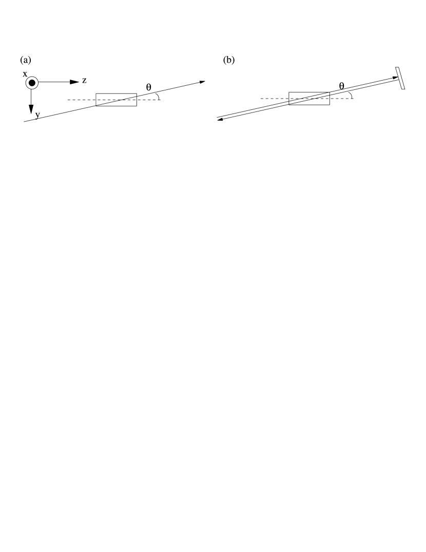
Figure 1: (a) Setup for a single beam with intensity $I({\bm{r}})$ propagating in direction $\theta$; (b) Two plane waves counterpropagating in direction $\theta$, giving rise to a standing wave configuration in the propagation direction. The second one is obtained by a mirror reflection of the first one.

We consider the different probing configurations shown in Fig. 1. They lead to an effective interaction Hamiltonian of the form

$$H_{\rm int}^{\rm eff}=-a\int d{\bm{r}}A({\bm{r}})\hat{s}_{z}\hat{J}_{P}$$ (3)

where $\hat{J}_{P}=\hat{J}_{z}\cos\theta-\hat{J}_{y}\sin\theta$ and the intensity $A({\bm{r}})=I({\bm{r}})$ for a tilted beam shown in fig.  1 (a). Probing setup (b) leads to $A({\bm{r}})=2\cos^{2}[kr_{P}+\phi]$, where $r_{P}=z\cos\theta-y\sin\theta$ and $\phi$ is the spatial phase of the probing standing wave.

In general both the atomic spin vectors and the Stokes operators are functions of space and time coordinates. Neglecting retardation effects, we can integrate over the duration of the probe pulse (of the order of $\mu s$) and define a macroscopic Stokes operator $\hat{S}_{\alpha}=\int dt\hat{s}_{\alpha}$ where $\alpha=x,y,z$. We consider light initially polarized in the $x$- direction $\langle\hat{S}_{x}\rangle=N_{P}/2$ and $\langle\hat{S}_{y}\rangle=\langle\hat{S}_{z}\rangle=0$, where $N_{P}$ is the photon number. Heisenberg equations of motion for the atomic spin lead to $\hat{J}_{\alpha}({\bm{r}},t)\equiv\hat{J}_{\alpha}({\bm{r}})$ $\forall\alpha$ to first order in time, while the spin in the direction of the probe $\hat{J}_{P}$ is conserved to all orders. Due to the atom-light interaction, the Stokes operator performs a Faraday rotation in the plane perpendicular to propagation

$$\partial_{\bm{r}}\hat{S}_{y}=-a\hat{J}_{P}({\bm{r}})\frac{N_{P}}{2}A({\bm{r}}).$$ (4)

Integrating equation (4), we find that the light quadrature, defined by the Stokes operators $\hat{S}_{y}$, $\hat{X}_{S}=\sqrt{2/N_{P}}\hat{S}_{y}$ reads after propagation through the sample

$$\langle\hat{X}_{s}^{\rm out}\rangle=\langle\hat{X}_{s}^{\rm in}\rangle-\frac{\kappa}{\sqrt{N_{A}}}\int d{\bm{r}}\langle\hat{J}_{P}({\bm{r}})\rangle A({\bm{r}}),$$ (5)

where $\kappa^{2}=a^{2}N_{P}N_{A}/2$, being $N_{A}$ the total number of atoms. The fluctuations read

$$(\delta\hat{X}_{S}^{\rm out})^{2}=\frac{1}{2}+\frac{\kappa^{2}}{N_{A}}\int d{\bm{r}}A({\bm{r}})\int d{\bm{r}^{\prime}}A({\bm{r}^{\prime}})\langle\delta\hat{J}_{P}({\bm{r}})\delta\hat{J}_{P}({\bm{r}^{\prime}})\rangle,$$ (6)

where $\delta\hat{J}_{P}=\hat{J}_{P}-\langle\hat{J}_{P}\rangle$. Thus fluctuations of the light quadrature (polarization fluctuations) after crossing the atomic sample contain the photon shot noise plus a contribution proportional to second order correlations of the atomic spins. Experimentally, spin-spin correlations can be detected if their contribution in the polarization fluctuations is larger that the photon shot noise, which for a coherent initial source corresponds to $(\delta\hat{X}_{S}^{\rm in})^{2}=\frac{1}{2}$. To this end, the relevant parameter is $\kappa^{2}=\eta\alpha$ where $\alpha$ is the resonant optical depth of the sample and $\eta$ is the spontaneous emission probability [20, 22]. It can be shown that the optimal signal is obtained when $\eta$ is tuned to $\eta_{opt}=1/\sqrt{2\alpha}$ and $\kappa^{2}=\sqrt{\alpha/2}$ [30]. BEC clouds have typical optical depths of the order of a few hundreds, for which one obtains quantum fluctuations imprinted on light by the spin fluctuations which are significantly bigger than the photon shot noise.

Technically it might be challenging to fix the spatial phase of the probing light $\phi$ with respect to the trapping potential of the atoms in standing wave probing configuration (b). We assume that the average of the signal over various shots of the experiment leads to averaging over $\phi$. Under phase averaging, Eq. (6) reduces to

$$(\delta\hat{X}_{S}^{\rm out}(\bm{k}))^{2}=\frac{1}{2}+\frac{\kappa^{2}V}{4N_{A}}\left[4S_{m}(0)+S_{m}(2\bm{k})+S_{m}(-2\bm{k})\right].$$ (7)

Here we have introduced the magnetic structure factor

$$S_{m}(\bm{k})=\frac{1}{V}\int d\bm{r}\int d\bm{r}^{\prime}e^{i\bm{k}(\bm{r}-\bm{r}^{\prime})}\langle\delta\hat{J}_{P}({\bm{r}})~{}\delta\hat{J}_{P}({\bm{r}^{\prime}})\rangle$$ (8)

where $V$ is the volume of the system and $\bm{k}$ is the momentum of the probing standing wave. If the Hamiltonian of the system conserves the total spin along the probing direction $P$, as it will be the case in the following examples, then $S_{m}(0)=0$. Moreover, due to the commutation of $\delta\hat{J}_{P}({\bm{r}}$ at different locations, $S(-2\bm{k})=S(2\bm{k})$.

In atoms are trapped in a one dimensional optical lattice as considered in Section 4, the atomic spin field ($e.g.$ along the $z$ direction) is localized at lattice sites, and it is conveniently expressed as

$$\hat{J}_{z}({\bm{r}})=\frac{1}{2}\sum_{i}|w({\bm{r}}-{\bm{r}}_{i})|^{2}~{}\hat{m}_{i}$$ (9)

where $\sum_{i}$ runs over the sites of the optical lattice and $\hat{m}_{i}=(\hat{n}_{i\uparrow}-\hat{n}_{i\downarrow})/2$ where $\hat{n}_{i,\sigma}$ is the occupation of fermions with spin $\sigma$ at lattice site $i$. $w({\bm{r}}-{\bm{r}}_{i})$ is the Wannier function at lattice site $i$; in the following we will approximate it with a $\delta$-function for simplicity. If the probing standing wave is not phase-locked spatially to the one creating the optical lattice, averaging over the relative phase between the two leads to Eq. (7) which contains the lattice magnetic structure factor:

$$S_{m}({\bm{k}})=\frac{|\tilde{w}({\bm{k}})|^{4}}{L^{d}}\sum_{ij}e^{i\bm{k}\cdot(\bm{r}_{i}-\bm{r}_{j})}\left(\langle\hat{m}_{i}\hat{m}_{j}\rangle-\langle\hat{m}_{i}\rangle\langle\hat{m}_{j}\rangle\right).$$ (10)

where $\tilde{w}$ is the Fourier transform of the Wannier function, and $L$ is the linear dimension of the $d$-dimensional lattice. In the following we consider for simplicity $w({\bm{r}})\sim\delta({\bm{r}})$, and consequently we neglect the ${\bm{k}}$-dependence of $\tilde{w}$.

Hence the method proposed here gives direct access to the magnetic structure factor of the atomic sample. This piece of information is crucial in detecting the onset of spin-spin correlations in the strongly interacting phases of trapped atomic samples. The (pseudo)spin degree of freedom of spin-$S$ atoms is encoded in $2S+1$ internal hyperfine states which are populated in the atomic sample. A fundamental example of spin correlations is the antiferromagnetic phase emerging at low temperatures in a Mott insulator of spin-(1/2) bosons or fermions in an optical lattice [24, 25]. More exotic spin states appear in spin-1 bosons, including dimerized states in one dimensional optical lattices [26]. Moreover, recent proposals envision the dipolar coupling of a $S=1/2$ pseudospin degree of freedom of molecules dressed with microwaves [27]: the spin couplings realized in this way give rise to novel magnetic phases including, e.g., topological quantum order.

3 Three dimensional balanced Fermionic superfluids

We begin by considering superfluidity in an homogeneous two-component balanced 3D Fermi system with two-body contact attractive interactions. The presence of interactions leads to pairing between the different spins described by the pairing order parameter $\Delta({\bm{r}})=|g|\langle\hat{\psi}^{\dagger}_{\uparrow}({\bm{r}})\hat{\psi}^{\dagger}_{\downarrow}({\bm{r}})\rangle$, where the interaction strength $g\propto 2k_{F}a_{s}$, $a_{s}$ is the two-body scattering length, and $k_{F}$ is the Fermi vector. For an homogeneous balanced 3D gas $\langle\hat{\bm{J}}({\bm{r}})\rangle=0$ and the spin fluctuations are the same along all directions. Using Wick’s theorem, the fluctuations in $\hat{J}_{z}$ read

$$4\langle\delta\hat{J}_{z}({\bm{r}})\delta\hat{J}_{z}({\bm{r}^{\prime}})\rangle=\sum_{\sigma=\uparrow\downarrow}(\langle\hat{n}_{\alpha}({\bm{r}})\rangle\delta({\bm{r-r^{\prime}}})-|\langle\hat{\psi}_{\sigma}^{\dagger}({\bm{r}})\psi_{\sigma}({\bm{r}^{\prime}})\rangle|^{2})-2|\langle\psi^{\dagger}_{\uparrow}({\bm{r}})\psi^{\dagger}_{\downarrow}({\bm{r}^{\prime}})\rangle|^{2}.$$ (11)

The BCS formalism [6] describes the BCS-BEC crossover, characterized by different values of the scattering length $1/k_{F}a_{s}$, in terms of the Bogoliubov amplitudes $u_{\textbf{k}}^{2}(v_{\textbf{k}}^{2})=\frac{1}{2}\left(1\pm\frac{\textbf{k}^{2}-\mu}{\sqrt{\Delta^{2}+(\textbf{k}^{2}-\mu)^{2}}}\right)$ where the chemical potential $\mu$ and superfluid gap $\Delta$ are obtained from the simultaneous solution of the gap and number equations [28]:

$$\frac{1}{k_{F}a}=(\tilde{\mu}^{2}+\tilde{\Delta}^{2})^{1/4}P_{1/2}(x)$$ (12)

$$\frac{\pi}{4}=\tilde{\mu}(\tilde{\mu}^{2}+\tilde{\Delta}^{2})^{1/4}P_{1/2}(x)+(\tilde{\mu}^{2}+\tilde{\Delta}^{2})^{3/4}P_{-1/2}(x)$$ (13)

where $x=-\mu/(\mu^{2}+\Delta^{2})^{1/2}$, $\tilde{\Delta}=\Delta/\epsilon_{F}$, $\tilde{\mu}=\mu/\epsilon_{F}$ and $P_{\eta}(x)$ are the Legendre functions of the first kind.

We consider two types of probing configurations: a running Gaussian beam [Fig. 1(a)] and a phase-averaged standing-wave configuration [Fig. 1(b)]. A Gaussian probing beam has an amplitude profile $A({\bm{r}})=e^{-{|{\bm{r}}_{\perp}|^{2}}/{\sigma^{2}}}$, where ${\bm{r}}_{\perp}$ are the coordinates perpendicular to the propagation direction. When the light is macroscopically polarized in the $x$-direction propagating through the sample, it yields $\langle\hat{X}_{s}^{\rm out}\rangle=\langle\hat{X}_{s}^{\rm in}\rangle$ and

$$(\delta X^{\rm out}_{s}({\bf k}))^{2}-\frac{1}{2}=\frac{\kappa^{2}}{2}\left[1-\frac{V}{N_{A}}\int d{\bm{r}}~{}e^{-r_{\perp}^{2}/\sigma^{2}}\left(|I_{\uparrow\uparrow}(\bm{r})|^{2}+|I_{\downarrow\uparrow}(\bm{r})|^{2}\right)\right],$$ (14)

where

$$I_{\uparrow\uparrow}(\bm{r})=\frac{1}{(2\pi)^{2}}\int_{0}^{\infty}dk~{}k^{2}~{}v_{\bf k}^{2}~{}j_{0}(kr)$$

$$I_{\uparrow\downarrow}(\bm{r})=\frac{1}{(2\pi)^{2}}\int_{0}^{\infty}dk~{}k^{2}~{}v_{\bf k}u^{*}_{\bf k}~{}j_{0}(kr),$$ (15)

and $j_{0}$ is the Bessel function.

For a homogeneous probing set-up the total spin fluctuations are zero [29], while a finite Gaussian probe shows a finite value of the spin fluctuations.

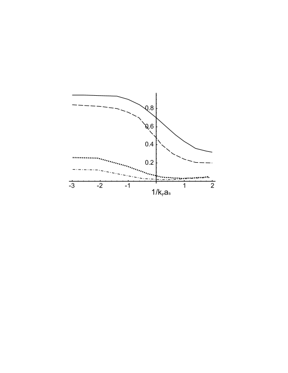
Figure 2: Spin fluctuations $((\delta X^{\rm out}_{s})^{2}-\frac{1}{2})/\frac{\kappa^{2}}{2}$ in the BCS ($a<0$)-BEC crossover for a Gaussian probing beam. Sizes $k_{F}\sigma=0.5$ (solid) , $k_{F}\sigma=1$ (dashed), $k_{F}\sigma=5$ (dotted) and $k_{F}\sigma=10$ (dot-dashed). Here $V=L^{3}$ with $Lk_{F}=100$.

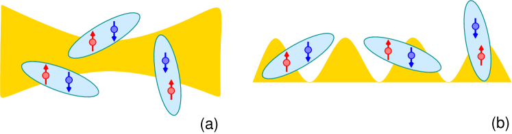
Figure 3: Probing schemes of spin fluctuations in paired fermionic gases. (a) Gaussian laser beam. (b) Standing wave.

Results in Fig. 2 show how the polarization fluctuations decrease with decreasing pair size along the BCS-BEC crossover. These results are in agreement with those of Ref. [31], and they reveal that the quantum fluctuations of the atomic spins imprinted on the light polarization are significantly suppressed when the characteristic pair size becomes smaller than the Gaussian beam waist $\sigma$. This is due to the simple fact that an $s$-wave pair is in a total spin singlet, and hence it does not contribute to the spin fluctuations of the atoms illuminated by the laser beam when it is fully contained within the beam waist. A sizable quantum noise imprinted in the polarization corresponds to the optimal situation in which the pair size is larger than or comparable to the beam waist, as sketched in Fig. 3(a). Yet a fundamental remark is necessary: in order to obtain a total excursion of order ${\cal O}(1)$ in the noise signal along the crossover, one needs to focus the laser to the experimentally challenging waists $\sigma\sim 1-10~{}k_{F}^{-1}$. In fact, for typical sample densities of order $n\sim 10^{13}$ atoms/cm³, one has $k_{F}^{-1}=(3\pi^{2}n)^{-1/3}\sim 150$ nm.

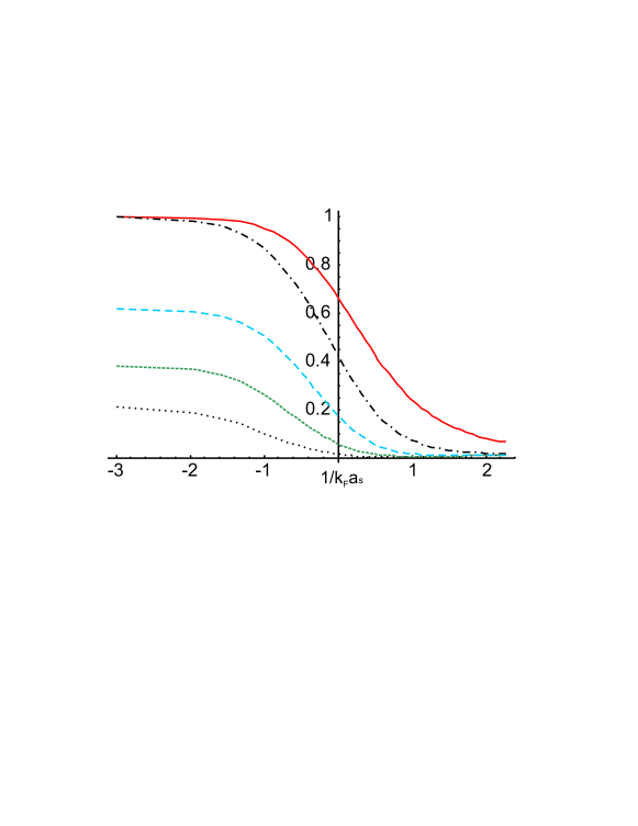
Figure 4: Spin fluctuations $((\delta X^{\rm out}_{s})^{2}-\frac{1}{2})/\frac{\kappa^{2}}{2}$ for different momenta of a phase-averaged probing standing wave $k$ in the BCS ($a<0$)-BEC crossover. This is also proportional to the magnetic structure factor $S_{m}(2k)$. Different lines correspond to $k/k_{F}=0.25,0.5,1,2,3$ in ascending order.

On the other hand, probing the system with a standing wave, as proposed in the previous section, gives high spatial resolution without the need of focusing a laser over prohibitively small length scales. Fig. 4 shows the magnetic structure factor $S_{m}(2k)V/N_{A}$, Eq. (8), at fixed wavevector $k$, obtained via the phase-averaged polarization fluctuations of two counter-propagating beams at wavevector $k$, as a function of the product $(k_{F}a_{s})^{-1}$. Strongly correlated spin fluctuations, recorded by the magnetic structure factor, are present over length scales related to the pair size, while the inter-pair spin correlations are vanishing. Hence the magnetic structure factor is very strongly affected by the shrinking of the pairs controlled by the scattering length, which gradually pushes the correlation length of spin fluctuations below the probe wavelength $2\pi/k$ (Fig. 3(b)). The light wavevectors $k/k_{F}$ = 0.25, 0.5, 1, 2, and 3, considered in Fig. 4, correspond to wavelengths $\sim$ 3770, 1885, 942, 471, and 314 nm respectively. The strongest excursion on the magnetic structure factor along the BCS-BEC crossover is observed for the largest wavevectors, which correspond to conventional laser wavelengths. The other wavelengths can be obtained effectively by crossing the counter-propagating beams at an angle, as we will discuss in a forthcoming publication.

The inflection point of the magnetic structure factor $S_{m}(2k)$ as a function of $(k_{F}a)^{-1}$ contains the information about the characteristic length $\xi_{l}$ beyond which the spatial average of spin fluctuations imprinted on the light polarization is strongly suppressed. The various scans of $S_{m}(2k)$ at fixed $k$ for varying $(k_{F}a)^{-1}$ allow to extract the $(k_{F}a)^{-1}$ location of the inflection point, and to reconstruct how the associated wavelength $\xi_{l}=2\pi/k$ depends upon $(k_{F}a)^{-1}$. This dependence is shown in Fig. 5. It is remarkable to see that the length $\xi_{l}$ follows the same behavior of the Pippard coherence length $\xi_{p}$ (up to a scaling factor) on the BCS side of the crossover, while it starts decreasing much faster around the unitarity limit. In this respect, it would be desirable to go beyond mean-field theory in the description of the strongly interacting regime, and to extend to that regime the comparison of the spatial features contained in the structure factor with the characteristic pair size.

The above analysis can be applied to BCS pairs as well as to molecules. Therefore QPS based on standing waves appears as a promising method to probe the internal structure of $s$-wave Feshbach molecules. Further analysis of the QPS signal in the case of, e.g., $p$-wave or $d$-wave pairing and Feshbach molecules will be the subject of future investigations.

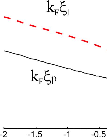
Figure 5: Solid line shows the Pippard coherent length ($\xi_{p}=1/\Delta\pi$) in $\log$-scale while the dashed line shows the corresponding length $\xi_{l}=2\pi/k_{0}$ where $k_{0}$ is the inflection point of the magnetic structure factor $S_{m}(2k)$.

4 Imbalanced Fermions in one dimension. Fingerprint of the FFLO phase

The possibility of exotic pairing in imbalanced fermionic mixtures has been recently the subject of a very intense research. In particular the mismatch between the Fermi momenta $k_{F\uparrow}$ and $k_{F\downarrow}$ of the two spin species can lead to the appearance of FFLO pairs with finite momentum $Q=|k_{F\uparrow}-k_{F\downarrow}|$. The experiments carried out so far seem to rule out this possibility in three dimensions, where phase separation of the gas into a balanced mixture (with conventional pairing) and a fully polarized gas of the remaining majority atoms is observed [7, 8]. On the other hand, analytical and numerical studies have rigorously proved the occurrence of a highly stable FFLO phase in one dimension [10, 11, 12, 13, 14].

In the following we concentrate on the case of one-dimensional imbalanced attractive fermions in an optical lattice, described by the 1D attractive Hubbard model in a parabolic trap:

$$H=-t\sum_{i,\sigma}\left(\hat{c}_{i,\sigma}^{\dagger}\hat{c}_{i+1,\sigma}+\rm{h.c.}\right)-U\sum_{i}\hat{n}_{i\uparrow}\hat{n}_{i\downarrow}$$ (16)

where $\hat{c}_{i,\sigma}^{\dagger}$ creates a fermion with spin $\sigma=\uparrow\downarrow$ at site $i$ , $\hat{n}_{i\sigma}=\hat{c}_{i,\sigma}^{\dagger}\hat{c}_{i,\sigma}$, $t$ is the hopping matrix and $U$ is the on-site attractive interaction.

We investigate this model by means of numerically exact quantum Monte Carlo simulations based on the Stochastic Series Expansion algorithm [32] in the canonical ensemble [33]. The temperature is set to reproduce the $T=0$ properties of the system. As pointed out in Section 2 the method of quantum polarization spectroscopy gives access to the magnetic structure factor Eq. (10), which is the quantity we calculate numerically with quantum Monte Carlo.

It is well known that, for a bipartite lattice, the attractive Hubbard model can be mapped onto the repulsive one via a particle-hole transformation on one of the two species, $\hat{c}_{i\uparrow}^{\dagger}=(-1)^{i}~{}\hat{c^{\prime}}_{i\uparrow}$, $\hat{c}_{i\downarrow}^{\dagger}=\hat{c^{\prime}}^{\dagger}_{i\downarrow}$. The fillings of the $c^{\prime}$ fermions are $n^{\prime}_{\uparrow}=1-n_{\uparrow}$ and $n^{\prime}_{\downarrow}=n_{\downarrow}$, and accordingly the Fermi wavevectors are transformed as $k^{\prime}_{F\uparrow}=\pi-k_{F\uparrow}$ and $k^{\prime}_{F\downarrow}=k_{F\downarrow}$. In particular the spin-spin correlation function of the attractive model maps onto the density-density correlation function of the repulsive one

$$C_{mm}(r)=\langle\hat{m}_{i}\hat{m}_{i+r}\rangle-\langle\hat{m}_{i}\rangle\langle\hat{m}_{i+r}\rangle=\frac{1}{4}\left(\langle\hat{n}^{\prime}_{i}\hat{n}^{\prime}_{i+r}\rangle-n^{\prime 2}\right)$$ (17)

where $\hat{n}^{\prime}_{i}=\hat{n}^{\prime}_{i\uparrow}+\hat{n}^{\prime}_{i\downarrow}$. The density-density correlation function for the repulsive Hubbard model has been investigated extensively in the past via Bethe Ansatz, and its general form is of the type

$$C^{\prime}_{nn}(r)=\langle\hat{n}^{\prime}_{i}\hat{n}^{\prime}_{i+r}\rangle-n^{\prime 2}=\sum_{l}B_{l}\frac{\cos(\alpha_{l}k^{\prime}_{F\uparrow}r+\beta_{l}k^{\prime}_{F\downarrow}r)}{r^{\Delta_{l}}}$$ (18)

where the various terms appearing in the sum are imposed by selection rules [34]. In particular it is found that $(\alpha_{l},\beta_{l})=(2,0),(0,2),(2,2),...$. To the best of our knowledge, the amplitudes $A_{l}$ of the various contributions have not been determined for the case of a spin-imbalanced Hubbard model at an arbitrary filling.

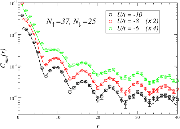
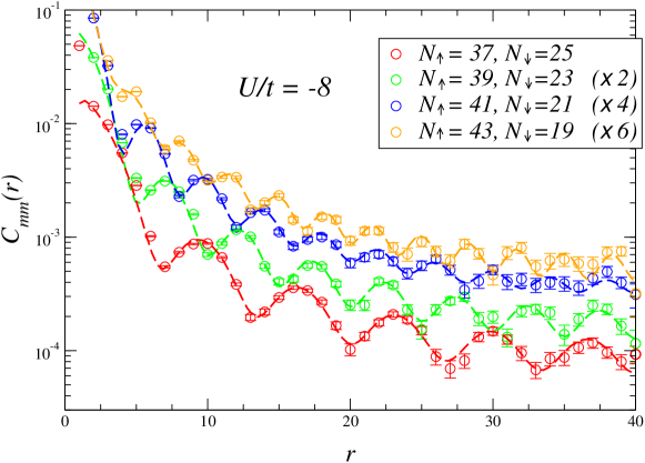
Figure 6: Spin-spin correlations in the 1D attractive Hubbard model with population imbalance for different polarization values and interaction strengths. The simulation data refer to a system size of $L=80$. To improve readability, in both panels some sets are multiplied by a constant (indicated in the set legends). The dashed lines are fits to the symmetrized form of Eq. (19). All results show consistency with the estimates $\Delta_{1}\approx 1.8$ and $\Delta_{2}\approx 2-2.2$, although the precision on the fitting coefficients does not allow us to extract the systematic dependence of the exponents on the polarization and interaction parameters.

The spin-spin correlation function for the attractive imbalanced 1D Hubbard model is shown in Fig. 6 for various values of the attraction and of the imbalance. Our numerical findings are all consistent with the expression

$$C_{mm}(r)=\frac{1}{4}~{}C^{\prime}_{nn}(r)\approx A_{1}~{}\frac{1}{r^{\Delta_{1}}}+A_{2}~{}\frac{\cos(2k^{\prime}_{F\uparrow}r+k^{\prime}_{F\downarrow}r)}{r^{\Delta_{2}}}=A_{1}~{}\frac{1}{r^{\Delta_{1}}}+A_{2}~{}\frac{\cos(2Qr)}{r^{\Delta_{2}}},~{}~{}$$ (19)

which, in the symmetrized form $C_{mm}(r)+C_{mm}(L-r)$, provides excellent fits to the finite-size numerical data.

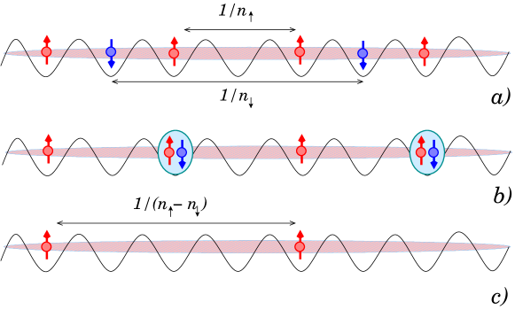
Figure 7: Sketch of the short-range properties of an imbalanced mixture of strongly attractive 1D fermions. $a)$ The two-component gas displays strong fluctuations towards a short-range crystalline-like arrangement with the majority spins at a maximum mutual distance $1/n_{\uparrow}$, and similarly for the minority spins. $b)$ The strongly attractive interaction leads to pairing fluctuations, which set the two short-range crystalline arrangement in phase spatially. From the magnetic point of view, pairing effectively erases some of the itinerant spins in the system, so that the resulting magnetic texture at short range has a characteristic length $\approx(n_{\uparrow}-n_{\uparrow})^{-1}$ and a characteristic associated wavevector $2\pi(n_{\uparrow}-n_{\uparrow})=2Q$.

This shows that the spin-spin correlation function of the attractive model is directly sensitive to the Fermi momentum mismatch $Q$ at which FFLO pairing occurs. A sketchy picture on the relationship between spin-spin correlations and FFLO pairing in the strong pairing limit is offered in Fig. 7. The FFLO state is effectively a mixture of bound pairs and of unbound majority atoms, which are mutually hardcore repulsive due to Pauli exclusion principle. Infinite repulsion in 1D leads to algebraically decaying charge-density-wave (CDW) correlations, namely the system displays strong fluctuations towards a local CDW state which very roughly corresponds to an equally spaced arrangement of pairs and excess $\uparrow$ particles [35]. From the point of view of the spin texture, considering bound pairs as spinless objects leaves out an algebraically decaying spin-density-wave arrangement which has a characteristic wavevector $2\pi(n_{\uparrow}-n_{\downarrow})=2Q$. Hence this argument shows that the $2Q$-modulation of spin-spin correlations is a direct fingerprint of pairing in an imbalanced mixture.

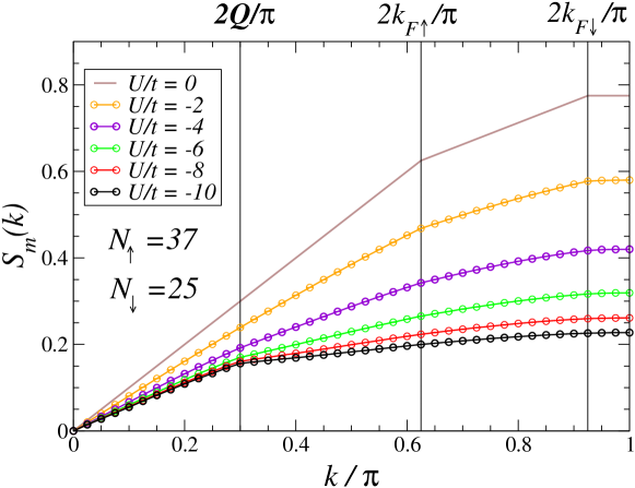
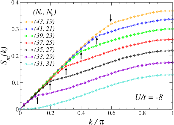
Figure 8: Magnetic structure factor in the 1D attractive Hubbard model with population imbalance for different polarization values and interaction strengths. The arrows in the lower panel mark the location $2Q/\pi$.

The $2Q$ modulation of spin-spin correlations translates into a pronounced kink at $k=2Q$ in the magnetic structure factor, as shown in Fig. 8 for various values of the attraction and of the imbalance. This kink is shown to be the only relevant feature in $S_{m}(k)$, and to be most pronounced for small imbalance. Fig. 8 also shows a comparison with the case of two non-interacting spin species $U=0$, which is exactly solvable. In that case the magnetic structure factor reads (for $k_{F\uparrow}>k_{F\downarrow}$)

$$S_{m}(k) = \frac{|k|}{\pi}~{}~{}~{}~{}~{}~{}~{}~{}~{}~{}~{}~{}~{}{\rm for}~{}~{}|k|\leq 2k_{F\downarrow}$$ (20)

$$= \frac{|k|+2k_{F\downarrow}}{2\pi}~{}~{}~{}~{}{\rm for}~{}~{}2k_{F\downarrow}\leq|k|\leq 2k_{F\uparrow}$$

$$= \frac{k_{F\uparrow}+k_{F\downarrow}}{\pi}~{}~{}~{}~{}~{}{\rm for}~{}~{}2k_{F\uparrow}\leq|k|\leq\pi~{}~{}.$$

This expression clearly exhibits two independent kinks at $2k_{F\uparrow}$ and $2k_{F\downarrow}$. As shown in Fig. 8, upon increasing the attraction $|U|$ among the two species, the two kinks of the non-interacting case disappear gradually, while the kink at $2Q$ appears clearly for $|U|/t\gtrsim 4$. The occurrence of a single kink at $2Q$ in the interacting model is hence a direct consequence of pairing.

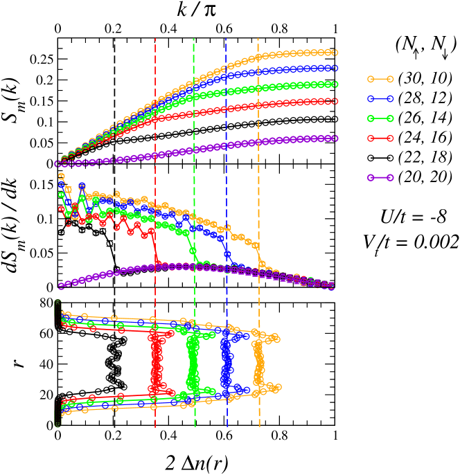
Figure 9: Upper panel. Magnetic structure factor in the trapped 1D attractive Hubbard model with population imbalance for different polarization values and interaction strengths.Middle panel. Momentum derivative of the magnetic structure factor. Lower panel. Corresponding density imbalance profiles, $\Delta n=n_{\uparrow}-n_{\downarrow}$. The dashed lines mark the correspondence between the central density imbalance in the trap, the position of the kink in the structure factor, and the corresponding jump in the structure factor derivative.

To make full contact with experiments, we also add a parabolic trap to the Hamiltonian Eq. (16)

$${\cal H^{\prime}}={\cal H}+V_{t}\sum_{i,\sigma}(i-L/2)^{2}~{}n_{i,\sigma},$$ (21)

where $L$ is the size of the lattice. We use similar parameters to those of Ref. [12], which shows clear evidence of FFLO pairing in terms of off-diagonal correlators. Fig. 9 remarkably shows that the kink feature in the magnetic structure factor survives to the presence of a trap. In particular, the presence of a kink is even better evidenced by the momentum derivative $dS_{m}(k)/dk$, which correspondingly exhibits a marked jump. The persistence of this feature in a trap is intimately connected with the fundamental fact that the density imbalance $\Delta n=n_{\uparrow}-n_{\downarrow}$ is almost constant over a significant portion of the trap center (although the density profiles of the two species independently are not as flat). Given that the location of the kink is only sensitive to the imbalance $Q=\pi\Delta n$, the persistence of the same $\Delta n$ over a large portion of the cloud protects the kink from smearing. Conversely, the position of the kink can be regarded as an efficient measure of the density imbalance in the trap center, which is not in principle known a priori. This is a valuable alternative to the direct in-situ phase contrast imaging recently applied to polarized Fermi gases [36] for the measurement of the density profiles of both species.

5 Conclusions

We have shown how spin-spin correlations of an attractive Fermi gas can be detected in a non-destructive way using spatially resolved quantum polarization spectroscopy (QPS). The atomic spins couple to the polarization degree of freedom of light and they imprint their correlations on the quantum fluctuations of the polarization, which can be measured using homodyne detection. When a standing wave is shone on the atomic sample, the measured signal allows a high resolution of spin-spin correlations in momentum space at the wavector of the standing wave.

Spin-spin correlations are shown to strongly characterize the superfluid phases of fermionic systems with attractive interactions. In a three-dimensional spin-balanced system the spatial structure of spin-spin correlations depends strongly on the pair size and hence it evolves strongly along the crossover from the BCS to the BEC regime: as a consequence, QPS is able to reveal the evolution of the characteristic pair size as a function of the scattering length. In a one-dimensional system with spin imbalance, the magnetic structure factor, recorded by the QPS signal, shows a kink at the difference between the Fermi vectors of the two spin species, providing a direct signature of finite-momentum Fulde-Ferrell-Larkin-Ovchinnikov pairing. The proposed experimental technique is most promising to detect the spin structure of exotic pairs and molecules, including e.g. $p$-wave and $d$-wave pairing, and to detect the magnetic phases which can be potentially realized by strongly correlated atoms and molecules loaded in optical lattices.

6 Acknowledgements

We acknowledge the support of the the European Commission through the“SCALA” project and STREP “NAMEQUAM”. the grant EMALI and FET grants HIDEAS, number FP7-ICT-221906 and COMPAS. Moreover we acknowledge the support coming from the grants of the Spanish Ministerio de Educación y Ciencia (FIS2005-0462, FIS2008-01236, Consolider Ingenio 2010 “QOIT”), the Catalan Goverment grant SGR00185, and the ESF-MEC Program “EUROQUAM” (“Fermix”).

References

- [1] Giorgini S, Pitaevskii L and Stringari S 2008 Rev. Mod. Phys. 63; Bloch I, Dalibard J, Zwerger W 2008 Rev. Mod. Phys. 80, 885; Ketterle W and Zwierlein M, Proceedings of the International School of Physics ”Enrico Fermi”, Course CLXIV, Varenna, June 2006
- [2] Regal C A, Greiner M and Jin D S 2004 Phys. Rev. Lett. 92, 040403.
- [3] Chin C, Bartenstein M, Altmeyer M, Riedl S, Jochim S, Hecker Denschlag J, and Grimm R 2004 Science 305 1128.
- [4] Kinast J, Turlapov A, Thomas J E, Chen Q, Stajic J, and Levin K 2005 Science 307 1296.
- [5] Zwierlein M W, Schunck C H, Schirotzek A, Ketterle W 2006 Nature 442, 54.
- [6] Leggett A J, 1980 J Phys C (Paris) 41, 7.
- [7] Zwierlein M W, Schirotzek A, Schunck C H, and Ketterle W 2006 Science 311, 492.
- [8] Partridge G B, Li W, Kamar R I, Liao Y, and Hulet R G 2006, Science 311, 503.
- [9] Fulde P and Ferrell A 1964 Phys. Rev. 135, A550; Larkin A and Ovchinikov Y, 1964 Zh. Eksp. Teor. Fiz. 47, 1136.
- [10] Batrouni G C, Huntley M H, Rousseau V G and Scalettar R T, 2008 Phys. Rev. Lett. 100, 116405; Casula M, Ceperley D M and Mueller E 2008 Phys. Rev. A 78, 033607.
- [11] Tezuka M and Ueda M 2008 Phys. Rev. Lett 100, 110403; Rizzi M et al. 2008 Phys. Rev. B 77, 245105.
- [12] Feiguin A F and Heidrich-Meisner F 2007, Phys. Rev. B 76 220508(R).
- [13] Drummond P 2007 Phys. Rev. Lett. 98, 070403; Orso G 2007 Phys. Rev. Lett. 98, 070402; Liu X-L, Hu H, and Drummond P D, 2007 Phys. Rev. A 76, 043605.
- [14] Ying Z, Cuoco M, 2008 Phys. Rev. Lett. 100, 140406; Asgari R 2008 Phys. Rev. A 77, 033604.
- [15] Wille E, Spiegelhalder E M, Kerner G, Naik D, Trenkwalder A, Hendl G, Schreck F, Grimm R, Tiecke G, Walraven J T M, Kokkelmans S J J M F, Tiesinga E, and Julienne P S 2008 Phys. Rev. Lett. 100, 053201 (2008).
- [16] Ni K K, Ospelkaus S, de Miranda M H G, Pe’er A, Neyenhuis B, Zirbel J J , Kotochigova S, Julienne P S, Jin D S, and Ye J 2008 Science 322, 231.
- [17] Altman E, Demler E, and Lukin M D 2004, Phys. Rev. A 70, 013603.
- [18] Greiner M, Regal C A, Stewart J T, and Jin D S 2005, Phys. Rev. Lett. 94, 110401.
- [19] Schunk C H, Shin Y, Schirotzek A, and Ketterle W 2008, Nature 454 739.
- [20] Sorensen J L, Hald J, and Polzik E S 1998 Phys. Rev. Lett., 80, 3847; Sherson J , Julsgaard B, and Polzik E S Adv. At. Mol. Opt. Phys., 54, November 2006, Academic Press.
- [21] Eckert K, Zawitkowski Ł, Sanpera A, Lewenstein M, and Polzik E S 2007 Phys. Rev. Lett. 98, 100404.
- [22] Eckert E, Romero-Isart O, Rodriguez M, Lewenstein M, Polzik E S and Sanpera A, 2008 Nature Physics 4, 50.
- [23] Julsgaard, ph-D thesis
- [24] Kuklov A B, and Svistunov B V 2003, Phys. Rev. Lett. 90, 100401.
- [25] Duan L M, Demler E, and Lukin M D 2003, Phys. Rev. Lett. 91, 090402.
- [26] Rizzi M, Rossini D, De Chiara G, Montangero S, and Fazio R 2005, Phys. Rev. Lett 95, 240404.
- [27] Micheli A, Brennen G K, and Zoller P 2006, Nature Phys. 6, 341.
- [28] Papaenbrock T and Bertsch G F 1999 Phys. Rev. C 59, 2052.
- [29] Mihaila B et al. 2005 Phys. Rev. Lett. 95, 090402.
- [30] Hammerer K, Molmer K, Polzik E S and Cirac J I 2004, Phys. Rev. A 70 ,044304.
- [31] Bruun G M, Andersen B M , Demler E and Sørensen A S 2008, arXiv:0809.0312.
- [32] Sandvik A W 1999, Phys. Rev. B 59, R14157; Syljuåsen O F 2003, Phys. Rev. E 67, 046701.
- [33] Roscilde T 2008, Phys. Rev. A 77, 063605.
- [34] Essler F H L, Frahm H, Göhmann F, Klümper A, and Korepin V E 2005, The One-Dimensional Hubbard Model, Cambridge.
- [35] A closer inspection into density correlations shows that, due to the attractive interactions, each bound pair is actually surrounded by a weak cloud of excess atoms, and viceversa the density-density correlations of atoms shows a weak modulation at the Fermi wavevector of the ones. Yet these aspects turn out to be irrelevant for the dominant behavior of spin-spin correlations.
- [36] Shin Y, Zwierlein M W, Schunck C H, Schirotzek A, and Ketterle W 2008, Phys. Rev. Lett. 97, 030401.