Coupled Mode Effects on Energy Transfer Rates in Two Temperature Plasmas

Abstract

We investigate the effects of collective modes on the temperature relaxation rates in fully coupled electron-ion systems. Firstly, the well-understood limit of weakly coupled plasmas is considered and the coupled mode formula within the random phase approximation is derived starting from the Lenard-Balescu kinetic equation. We show how the frequency integration can be performed by standard methods without applying additional approximations. Due to the well-defined approximation scheme, the results can serve as a benchmark for more approximate theories and numerical simulations in this limit. The coupled mode electron-ion transfer rates show a considerable reduction compared to the Fermi-Golden Rule approach for certain parameters and very small changes for other systems. We demonstrate how these coupled mode effects are connected to the occurance of ion acoustic modes and under which conditions they occur. Interestingly, coupled mode effects can also occur for plasmas with very high electron temperatures; a regime, where the Landau-Spitzer approach is believed to give accurate results. Finally, we extend the approach to systems with strongly coupled ions by applying static local field corrections. This extension can substantially increase the coupled mode effects.

I Introduction

Experimental characterization of warm dense matter and strongly coupled plasmas becomes increasingly powerful with the development of new methods for the creation and probing of such states. For instance, x-ray scattering allows not only for the measurement of equation of state data (like in traditional shock wave experiments, see, e.g., Refs. CDCG_98 ; KHBH_01 ), but also to obtain structural, dynamic, and collective properties of matter RWSW_00 ; RGBD_07 ; GLNL_07 ; GGGV_08 ; KNCD_08 . With these new possibilities, one is now able to probe the physics of high energy density matter as it is encountered during inertial confinement fusion or in the interior of planets.

The creation of the these high energy density states in the laboratory requires large and fast energy inputs into matter. Since static techniques, like diamond anvil cells, are restricted to lower temperatures and densities by the given stress point of the material, one relies on dynamic experiments applying intense particle beams and lasers to heat and compress the material under investigation. Inevitably, highly nonequilibrium states are produced with the energy being pumped mainly either into the ion or the electron subsystem. Such states are of great interest by itself since they reveil many dynamic and collective properties of the system more clearly.

A good understanding of nonequilibrium states is also needed for definitive measurements of equilibrium properties. After a very short time of approximately an inverse plasma frequency, electrons and ions have established temperatures within their subsystems and a full kinetic description is not necessary later on. Apart from the final hydrodynamic response, temperature equilibration thus takes the longest time of all relaxation processes driven by the intial energy deposition and defines the minimum time delay between the pump and probe pulses needed for equilibrium measurements.

Temperature equilibration is furthermore interesting since its time scale is experimentally accessible. Indeed, experiments investigating dense plasmas, both laser- and shock-produced, found relaxation times considerably longer than predicted by classical Landau-Spitzer formula CNXF_92 ; NCXF_95 . Two shortcomings of this easy-to-use approach were associated with these discrepancies: the neglect of collective excitations and the use of classical collisions. A full quantum binary collision approach yields however even larger energy transfer rates GMS_02 ; GMS_02b ; com_1 . Considering independent collective modes in the electronic and ionic subsystems within the Fermi-Golden-Rule (FGR) approach yields rates very close to the Landau-Spitzer results HZRD_01 . Therefore, collective modes in fully coupled electron-ion systems seem to be the only candidate to explain the lower electron-ion energy transfer measured.

More complex descriptions of temperature relaxation involve the interplay of all contributions to the internal energy. In addition to the kinetic parts interesting for temperature relaxation, correlations and exchange energies GM_05 ; GMBS_03 ; GBS_06 and the ionisation equilibrium including excitations OBBK_96 ; BSP_98 ; GGBS_06 can be important. The latter processes have been shown to considerable influence the relaxation under conditions far from equilibrium, but are not sufficient to explain the measured slower temperature equilibration.

Here, we assume ionisation, recombination, and charge transfer processes to be completed and concentrate on the electron-ion energy transfer including collisions and collective excitations in a fully coupled system. We use a quantum statistical description which avoids any ad hoc cutoffs known from classical descriptions and enables us to rigorously derive formulas for the energy transfer rates within a given approximation scheme.

The occurance and magnitude of coupled mode effects on temperature relaxation are still under discussion (see Refs. DP_98 ; D_01 ; DM_07 ; DM_08 ; GG_08 ). In the beginning, we therefore consider weakly coupled plasmas, where the classical coupling parameter, $\Gamma_{\!j}\!=\!Z_{\!j}^{2}e^{2}/a_{\!j}\,k_{\!B}T_{\!j}$ with $a_{\!j}\!=\!(3/4\pi n_{\!j})^{1/3}$ is small for all species. In this limit, we can employ the well-established random phase approximation (RPA) to describe the dynamic response of fully coupled systems and the quantum version of the Lenard-Balescu equation L_60 ; B_60 ; brown on the kinetic level. We show that the weak coupling version of the coupled mode formula derived by Dharma-wardana & Perrot DP_98 follows. Moreover, we re-write the density response functions of their approach in terms of dielectric functions and obtain a form that can be evaluated by standard integration procedures.

Under certain conditions, we observe a lowering of the energy transfer rates compared to the Landau-Spitzer and the FGR approaches in the order of a factor of two. These differences are connected to the occurance of ion acoustic modes and a related redistribution of weight in the dynamic density response toward smaller frequencies. This fact also explains why a simpler approximation like FGR is suitable for other parameters. The most striking fact is that coupled mode effects can occur also for very high electron temperatures where the Landau-Spitzer approach is believed to work well.

We have good control over our approximation scheme. The results in the well-understood weak coupling limit can thus serve as a benchmark for more approximate approaches. In particular, numerical simulations such as applied in Refs. GGMM_08 ; JFCC_08 should be tested against these analytic results since they are based on classical mechanics and apply pseudo-potentials to approximately incorporate the qantum nature of the electrons as an uncontrolled approximation.

As an extension to the RPA scheme, we consider strongly coupled ions where the additional correlation effects are treated on the level of static local field corrections. The additional shifts in the mode structure can further reduce the electron-ion energy transfer. For compressed silicon as discussed in Ref. NCXF_95 , we report large reductions although coupled mode effects on the RPA level do not change the rates much. In addition, we discuss the influence of degeneracy, mass and ion charge.

II Energy Transfer Rates

II.1 General Kinetic Description

Changes of the kinetic energy of species $a$, that is $\dot{E}_{a}$, are fully determind by the changes of the one-particle Wigner distribution of the species $f_{a}$

$$\frac{\partial}{\partial t}E_{a} \!\!=\!\! \int\frac{d{\mbox{\boldmath$p$}}}{{(2\pi\hbar)^{3}}}\,\frac{p^{2}}{2m_{a}}\,\frac{\partial}{\partial t}f_{a}({\mbox{\boldmath$p$}},t)$$ (1)

$$\!\!=\!\! \int\frac{d{\mbox{\boldmath$p$}}}{{(2\pi\hbar)^{3}}}\,\frac{p^{2}}{2m_{a}}\,\sum_{b}I_{ab}(p,t)\,.$$

In the second line, two-particle collision integrals $I_{ab}$ were introduced by using a general kinetic equation for homogeneous and isotropic systems: $\partial f_{a}/\partial t=\sum_{b}I_{ab}$. The equations for the electron and ion species are coupled by the collision integrals $I_{ei}=I_{ie}$ and, thus, the total energy of the plasma is conserved.

There exists a hierachy of approximations for the collision integrals $I_{ab}$ brown which via Eq. (1) also defines the quality of the related energy transfer rates. The different kinetic equations can be devided into two classes: the first describes the interactions by binary collisions only (Landau equation L_36 and Boltzmann-like equation D_84 ), the second includes also collective effects such as dynamic screening (Lenard-Balescu-type kinetic equations L_60 ; B_60 ). The mutual influence of electrons and ions via the common dielectric function of the plasma (coupled collective modes) is here included and predicted to strongly modify the energy transfer in two-temperature plasmas DP_98 ; D_01 .

II.2 Classical and Quantum Binary Collisions

The easiest approximation for the two-particle collision integral considers classical binary collisions. The corresponding energy transfer rates were derived in the first description of temperature relaxation by Landau and Spitzer L_36 ; S_62

$$\frac{\partial}{\partial t}E^{LS}_{e\to i}=\frac{3}{2}n_{e}k_{B}\frac{T_{i}-T_{e}}{\tau_{ei}}$$ (2)

with the electron-ion relaxation time

$$\tau_{ei}=\frac{3m_{e}m_{i}}{8\sqrt{2}n_{i}Z_{i}^{2}e^{4}\ln\Lambda}\left(\frac{k_{B}T_{e}}{m_{e}}+\frac{k_{B}T_{i}}{m_{i}}\right)^{3/2}\,.$$ (3)

The plasma properties define the Coulomb logarithm $\ln\Lambda$, where $\Lambda$ is the ratio of the maximum and minimum impact parameters. Here, we use a Coulomb logarithm of the form $\ln\Lambda\!=\!0.5\ln(1+\lambda_{e}^{2}/(\varrho_{\perp}^{2}+\lambda_{dB}^{2}))$ with the electron screening length $\lambda_{e}\!=\!(k_{B}T_{e}/4\pi e^{2}n_{e})^{1/2}$, the distance of closest approach $\varrho_{\perp}\!=\!Z_{b}e^{2}/m_{e}v_{th}^{2}$, the deBroglie wave length $\lambda_{dB}\!=\!\hbar/m_{e}v_{th}$, and the thermal velocity $v_{th}\!=\!(k_{B}T_{e}/m_{e})^{1/2}$. This form, which follows by considering hyperbolic orbits of the electrons, has the advantage to give non-negative results even for the dense plasmas considered in this paper. For a more extensive discussion see Ref. GMS_02 .

The Landau-Spitzer formula (3) suffers from a number of deficits. The most crucial one is the classical description of electron-ion collisions which may result in negative Coulomb logarithms and rates. Well-defined energy transfer rates in the binary collision approximation can however be derived based on the collision integral of the quantum Boltzmann equation zhdan ; GMS_02 . If the collision cross sections needed are calculated from the two-particle Schrödinger equation, these rates consider strong electron-ion collisions as well but collective excitations cannot be included since statically screened interactions are used. Most binary collision approaches are also limited to systems with nondegenerate electrons due to the way the collision cross sections are calculated.

II.3 Collective Modes in Weakly Coupled Plasmas

The collective excitations of a weakly coupled plasma are fully accounted for in the well-known random phase approximation (RPA). Since the electrons and ions are treated as one combined system in this approach, their mutual influence is naturally accounted for and, so called, coupled collective modes arise. This becomes particularly clear when considering the dielectric function on the RPA level that includes a sum over all species

$$\varepsilon^{RPA}(k,\omega)=1-\sum_{a}V_{aa}(k)\,\chi_{aa}^{0}(k,\omega)\,,$$ (4)

where $\chi_{aa}^{0}$ is the free density response function for the particles of species $a$.

The kinetic equation corresponding to the RPA is the Lenard-Balescu equation L_60 ; B_60 . Here, we will use its quantum generalization that accounts for degeneracy brown . The energy transfer rates are again obtained by inserting the appropriate collision integral into the energy balance (1). Details of the derivation can be found in Appendix A and the final result is

$$\frac{\partial}{\partial t}E^{CM}_{e\to i} \!\!=\!\! -4\hbar\sum\limits_{i}\int\!\frac{d{\mbox{\boldmath$k$}}}{{(2\pi\hbar)^{3}}}\!\int\limits_{0}^{\infty}\frac{d\omega}{2\pi}\;\omega\,\left|\frac{{\mathrm{V}}_{ei}(k)}{\varepsilon^{RPA}(k,\omega)}\right|^{2}$$

$$\times\mathop{\mathrm{Im}}\chi^{0}_{ee}(k\omega)\,\mathop{\mathrm{Im}}\chi^{0}_{ii}(k\omega)\,\Big{[}n_{B}^{e}(\omega)-n_{B}^{i}(\omega)\Big{]}\,.$$

$n_{B}^{a}(\omega)\!=\![\exp(\hbar\omega/k_{B}T_{a})-1]^{-1}$ is a Bose function that characterises the occupation number of the collective modes and $V_{ei}(k)\!=\!4\pi Ze^{2}/k^{2}$ is the pure Coulomb potential. The zeros of the total dielectric function in the denominator determine the collective excitations of the fully coupled system. Thus, the energy transfer rate (LABEL:cm_transf) carries the label ‘CM’ for coupled mode. It is applicable for weakly coupled plasmas without any restriction with respect to degeneracy. For weakly coupled plasmas, equation (LABEL:cm_transf) is equivalent to the CM formula given by Dharma-wardana & Perrot (see Eq. (50) in Ref. DP_98 ) which is demonstrated in Appendix B.

We would like to emphasis again that expression (LABEL:cm_transf) represents a CM formula for the energy transfer rates in weakly coupled, two-temperature systems. It was derived from the well-established (quantum) Lenard-Balescu equation in RPA without further approximations. Therefore, it can serve as a benchmark for more approximate approaches and numerical simulations in the weak coupling limit.

One of the more approximate, but easier to calculate, approaches for the energy transfer rates is the Fermi golden rule (FGR) approach. Here, electrons and ions are treated as separate subsystems. Accordingly, both subsystems have their own distinct dielectric functions $\varepsilon_{a}^{RPA}\!=\!1\!-\!V_{aa}\,\chi_{aa}^{0}$. The expression for the energy transfer rates reflects this fact by having a product of these dielectric functions in the denominator DP_98 ; G_05

$$\frac{\partial}{\partial t}E^{FGR}_{e\to i} \!\!=\!\! -4\hbar\sum\limits_{i}\int\!\!\frac{d{\mbox{\boldmath$k$}}}{{(2\pi\hbar)^{3}}}\!\int\limits_{0}^{\infty}\frac{d\omega}{2\pi}\;\frac{\omega\,\left|{\mathrm{V}}_{ei}(k)\right|^{2}}{\left|\varepsilon_{e}(k,\omega)\right|^{2}\left|\varepsilon_{i}(k,\omega)\right|^{2}}$$

$$\times\mathop{\mathrm{Im}}\chi^{0}_{ee}(k\omega)\,\mathop{\mathrm{Im}}\chi^{0}_{ii}(k\omega)\,\Big{[}n_{B}^{e}(\omega)-n_{B}^{i}(\omega)\Big{]}\,.$$

It can be shown that the FGR rate reduces to Landau-Spitzer (LS) if classical expressions for the dielectric function are used HZRD_01 ; G_05 .

Although both, the CM expression (LABEL:cm_transf) and the FGR formula (LABEL:fgr_transf), contain effects of collective excitations, they describe quite different systems since the spectra of the modes do not agree. To evaluate the corresponding differences in the energy transfer rates is the main purpose of this paper.

II.4 Incorporation of Strong Coupling Effects

In dense plasmas, the Coulomb correlations between the particles can strongly effect the mode spectrum and scattering cross sections. The extensions towards strong coupling in the CM formula were already given in the original derivation by Dharma-wardana & Perrot DP_98 .

Strong electron-ion collisions may be accounted for by a weaker electron-ion pseudo-potential: ${\mathrm{V}}_{ei}(k)\to{\mathrm{U}}_{ei}(k)$. Spatial correlations, in particular in the ionic subsystem, can be described by a dielectric function that includes local field corrections. Here, we will use static local field correction (SLFC) for the strongly coupled ions only. In this case, the ionic dielectric function reads I_82

$$\varepsilon_{i}(k,\omega)=1-\frac{V_{ii}(k)\chi^{0}_{ii}(k,\omega)}{1+V_{ii}(k)G_{ii}(k)\chi^{0}_{ii}(k,\omega)}\,.$$ (7)

The local field factor $G_{ii}(k)$ is connected to the ionic structure factor $S_{ii}(k)$ via

$$G_{ii}(k)=1-\frac{k_{B}T_{i}}{n_{i}V_{ii}(k)}\left(\frac{1}{S_{ii}(k)}-1\right)\,.$$ (8)

The spatial correlations in $S_{ii}(k)$ can be calculated by molecular dynamics or Monte Carlo simulations as well as integral equations like the hypernetted chain approach HM_book .

It should be mentioned here that the changes due to SLFC influence only the CM rates. Within the FGR approach, the $\omega$-integration is essentially determined by the f-sum rule HZRD_01 ; G_05 which gives the same result independent of the approximation level used. Therefore, strong coupling effects are always included in the FGR rates.

III Evaluation of the Coupled Mode and FGR Expressions

The occurance of collective modes in the systems is connected with zeros in the dielectric function and results in sharp peaks in the $\omega$-integration. These peaks prohibit the evaluation of Eqs. (LABEL:cm_transf) and (LABEL:fgr_transf) by standard integration routines. We will first show under which conditions these modes occur and then describe the numerical integration procedure.

III.1 Mode Structure in CM and FGR

The electron modes have the well-known acoustic and plasmon-like branches and are almost unaffected by the presence of the ions. While the acoustic branch is strongly damped, the plasmon results in a sharp peak at the plasmon frequency $\omega_{e}\!\approx\!(4\pi e^{2}n_{e}/m_{e})^{1/2}$ (see Fig. 1). However, these modes are practically not included in the $\omega$-integration which is effectively limited by the function $\mathop{\mathrm{Im}}\chi^{0}_{ii}(k,\omega)$ to frequencies less than the ion plasma frequency $\omega_{i}\!\approx\!(4\pi Z_{i}^{2}e^{2}n_{i}/m_{i})^{1/2}$.

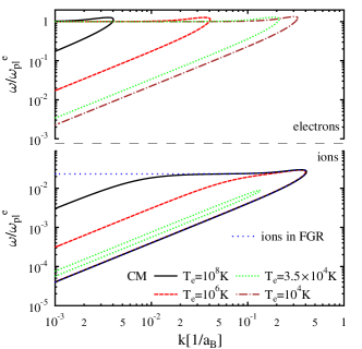
Figure 1: (Color online) Dispersion relations, $\mbox{Re}\varepsilon(k,\omega)\!=\!0$, for the modes in a hydrogen plasma with an ion temperature of $T_{i}\!=\!10^{4}\,$K, a density of $n\!=\!10^{22}\,$cm^-3, and different electron temperatures. Frequencies are normalized to the electron plasma frequency. In the FGR approach, there exists an electron and an ion plasmon mode (upper blue dotted line) whereas all ion modes become acoustic in the coupled system.

The ionic modes used in the FGR and CM approaches are qualitatively different. For small momenta, the ion subsystem in FGR has always a plasmon mode which is similar to the electron plasmon (just scaled by $Z_{i}$ and $m_{i}$) as well as an acoustic mode. The coupling between the electronic and ionic subsystems as included in the CM formula leads to screening of the ionic plasmon mode which therefore turns into a weakly damped upper acoustic branch of the ionic spectrum. The finite mode frequency at $k\!=\!0$ is thus shifted to much smaller frequencies that linearly increase with $k$. Interestingly, this new acoustic branch becomes more plasmon-like for larger temperature differences and momenta and coincides with the prediction for an isolated ion system in the unscreened limit with $T_{e}\!\to\!\infty$. For the important small $k$ values, the modes are however for all finite electron temperatures acoustic (in contrast to the FGR modes).

Fig. 1 also clearly demonstrates that the ionic modes in the coupled system cease to exist if the temperature difference, $T_{e}\!-\!T_{i}$, becomes too small. The mode frequency is, for small $k$, in very good approximation given by the zeros of the real part of the dielectric function. While the product of dielectric functions in the FGR approach has always zeros, the summation over species in the full dielectric function (4) puts strict limits to the occurrence of ionic modes and changes their location in $\omega$-space; a fact that is crucial for the understanding of the CM effect on the energy relaxation.

To estimate under which conditions ion acoustic modes in the coupled plasma occur, we have to balance the electronic terms which can be treated statically and the frequency-dependent ionic part. It is well-known that a zero in the real part of the full dielectric function can be achieved under the condition $T_{i}\!\ll\!T_{e}$ LL_81 . A more precise analysis (see Appendix C) shows that either of the relations VG_08

$$T_{i}\leq 0.27\cdot Z_{i}\,T_{e} n_{e}\Lambda_{e}^{3}\ll 1\;,$$ for

$$T_{i}\leq 0.27\cdot Z_{i}\,T_{F} n_{e}\Lambda_{e}^{3}\gg 1$$ for (9)

must hold to allow for an ion acoustic mode in coupled electron-ion systems. The upper case gives the limit for nondegenerate electrons while the second line sets the limit for highly degenerate electrons ($\Lambda_{e}^{2}=2\pi\hbar/m_{e}k_{B}T_{e}$ is the thermal wave length). In the high density case, the important temperature scale is thus defined by the electron Fermi temperature $T_{F}\!=\!\hbar^{2}(3\pi^{2}n_{e})^{2/3}/2k_{B}m_{e}$. Accordingly, sharp ion acoustic modes may also occur for $T_{e}\!<\!T_{i}$ if the electron density is high enough.

III.2 Evaluating the FGR Formula

The FGR formula for the energy transfer rates (LABEL:fgr_transf) always features sharp peaks at small wave numbers that are roughly located at the ion plasmon frequency. The exact value of the mode frequency $\Omega$ can be easily obtained numerically. To avoid the sharp peaks, these contributions around the location of the mode are cut out. The cut out contributions can be easily calculated from the differences to an $\omega$-integral that allows for an evaluation by the f-sum rule KSG_90 . Thus, we have to compute

$$\quad\int\limits_{0}^{\infty}\frac{d\omega}{2\pi}\,\omega\,\Delta N_{ei}(\omega)\frac{\mathop{\mathrm{Im}}\varepsilon_{e}(\omega)\,\mathop{\mathrm{Im}}\varepsilon_{i}(\omega)}{\big{|}\varepsilon_{e}(\omega)\big{|}^{2}\,\big{|}\varepsilon_{i}(\omega)\big{|}^{2}}$$

$$\;\,=\int\limits_{0}^{\infty}\frac{d\omega}{2\pi}\,\omega\,\frac{\mathop{\mathrm{Im}}\varepsilon_{i}(\omega)}{\big{|}\varepsilon_{i}(\omega,t)\big{|}^{2}}\,F(\omega)\left[1-\frac{F(\Omega)}{F(\omega)}\right]-\frac{\pi}{2}\omega_{i}^{2}F(\Omega)\,.$$

Here, $\Delta N_{ei}(\omega)\!=\!n_{B}^{e}(\omega)\!-\!n_{B}^{i}(\omega)$ is the difference in the mode occupation numbers. The function $F(\omega)$ includes the electronic dielectric functions and $\Delta N_{ei}(\omega)$, that is, $F(\omega)\!=\!\Delta N_{ei}(\omega)\mathop{\mathrm{Im}}\varepsilon_{e}(\omega)/|\varepsilon_{e}(\omega)|^{2}$. In this way, the sharp plasmon peak has been removed and then treated exactly. All remaining integrals are over smooth functions.

III.3 Evaluating the CM Expression

Unfortunately, an evaluation as for the FGR formula is impossible for the CM integrand. Here, the electronic and ionic parts do not separate and one cannot expand the integrand into a full dielectric function needed for the f-sum rule.

The functions under the $\omega$-integral can, however, be rearranged to allow for an integration with standard routines. For this aim, we artificially decompose the total dielectric function into an electron and an ion part

$$\varepsilon^{RPA}(k,\omega)=1\!\!\! +[\mathop{\mathrm{Re}}\varepsilon_{e}(k,\omega)-1]\!\!\! +\mathop{\mathrm{Im}}\varepsilon_{e}(k,\omega)\;\,$$ (11)

$$+[\mathop{\mathrm{Re}}\varepsilon_{i}(k,\omega)-1]\!\!\! +\mathop{\mathrm{Im}}\varepsilon_{i}(k,\omega)\,.$$

Then, we express the density respose functions in terms of dielectric functions: $\mathop{\mathrm{Im}}\varepsilon_{a}^{RPA}(k,\omega)\!=\!V_{aa}(k)\mathop{\mathrm{Im}}\chi_{aa}^{0}(k,\omega)$. In the case of a Coulombic interaction, $V_{ei}^{2}=V_{ii}V_{ee}$ holds and can be used to do the transformation above. The $\omega$-integral has now the form

$$I_{\omega}=\int\limits_{0}^{\infty}\frac{d\omega}{2\pi}\,\omega\,\Delta N_{ei}(\omega)\frac{\mathop{\mathrm{Im}}\varepsilon_{e}(k,\omega)\,\mathop{\mathrm{Im}}\varepsilon_{i}(k\omega)}{\big{|}\varepsilon^{RPA}(k,\omega)\big{|}^{2}}\,.$$ (12)

This form can still have very sharp peaks at the positions of the weakly damped upper ion acoustic modes. However, these peaks are limited in height since the real part of the total dielectric functions vanish at the mode frequency and we have

$$\lim_{\mathop{\mathrm{Re}}\varepsilon\to 0}\frac{\mathop{\mathrm{Im}}\varepsilon_{e}(k,\omega)\,\mathop{\mathrm{Im}}\varepsilon_{i}(k,\omega)}{\left|\varepsilon^{RPA}(k,\omega)\right|^{2}}\qquad\qquad\qquad\quad$$

$$=\frac{\mathop{\mathrm{Im}}\varepsilon_{e}(k,\omega)\,\mathop{\mathrm{Im}}\varepsilon_{i}(k,\omega)}{\left|\mathop{\mathrm{Im}}\varepsilon_{e}(k,\omega)+\mathop{\mathrm{Im}}\varepsilon_{i}(k,\omega)\right|^{2}}<1\,.$$ (13)

This rearrangement makes a brute force approach for integrating the CM equation (12) feasible since extremely narrow peaks have now no contribution to the integral.

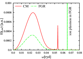
Figure 2: (Color online) Examples the combination of dielectric functions in the $\omega$-integrand of the CM and FGR expressions, i.e., $f_{CM}\!=\!\mbox{Im}\varepsilon_{e}\mbox{Im}\varepsilon_{i}/|\varepsilon|^{2}$ and $f_{FGR}\!=\!\mbox{Im}\varepsilon_{e}\mbox{Im}\varepsilon_{i}/|\varepsilon_{e}|^{2}|\varepsilon_{i}|^{2}$, respectively. Considered is a small wave number of $k\!=\!a_{B}^{-1}$ and a hydrogen plasma with $T_{i}\!=\!10^{5}\,$K, $T_{e}\!=\!10^{6}\,$K, and $n\!=\!10^{24}\,$cm^-3. Note: the height of the ion plasmon peak in the FGR approach is 1500 a.u.

III.4 Results of the $\omega$-integration

Example of the $\omega$-integrands for the two approaches are plotted in Fig. 2. The wave number has been chosen small enough that the ion acoustic mode exists in the CM approximation. It is clearly visible that the ion mode is shifted to lower frequencies. Moreover, the height of this peak has reduced dramatically indicating much larger damping. Although the particle excitation (left broad peak) is increasing, it cannot compensate the loss in weight. For a pure ion system, as in the FGR approach, almost the entire contribution stems from the plasmon peak whereas the main contribution to the CM integral comes from the particle peak.

The above points are the basics to understand the lowering of the energy transfer due to coupled collective modes. Figure 3 demonstrates that the CM effect is caused by differences at small wave numbers. Here, the ion acoustic mode exists and the influence of the electrons shifts the weight to smaller $k$ as shown in Fig. 1. Thus, the overall contributions to the CM integral are of the same order as the particle peak of the FGR which itself is negligible compared to the ion plasmon peak. Accordingly, small $k$-values give almost no contribution in the CM expression compared to the FGR results as shown in Fig. 3. If these small $k$ are important, significantly reduced CM rates, compared to FGR, can be expected. For large momentum transfers $k$, the situation is different: here, the ion acoustic mode (in CM) and the plasmon mode (in FGR) do not exist anymore and the $\omega$-integrals of both approaches merge. If such larger $k$ dominate in expressions (LABEL:cm_transf) and (LABEL:fgr_transf), no coupled mode effects can be expected.

IV Results and Discussion of the Energy Transfer Rates

We now turn to the analysis of energy transfer rates in dense two-temperature plasmas applying the CM, the FGR and the LS approaches. We consider a variety of situations typical for laser- as well as shock-produced plasmas. First, we will concentrate on weakly coupled plasmas and describe the plasma within the random phase approximation. Based on the methods presented above, this allows us to calculate the CM energy transfer rates on a well-established approximation level (similar to that of the quantum Lenard-Balescu equation) without any further approximations. In a second step, we will include static local field corrections to extend the CM approach to plasmas with strongly coupled ions.

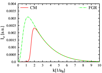
Figure 3: (Color online) Examples for the $\omega$-integral in the CM and FGR expressions for hydrogen as in Fig. 2.

IV.1 Results for Hydrogen within RPA

In a first example, hydrogen at a high density, as needed for the simulation of inertial confinement fusion scenarios, is considered in Fig. 4. In this example, we have relatively warm ions and hotter electrons (the range of $T_{e}$ has been extended to see the limiting behavior). All approaches show similar curves: i) a strong increase of the rates when the electron temperature is just a few times the ion temperature, ii) maximum of the energy transfer, and iii) a LS-like asymptotic reduction of the energy transfer $\sim T_{e}^{1/2}$. However, considerable quantitative differences arise when comparing the approximation levels presented.

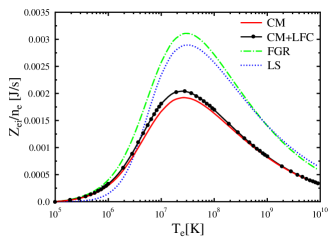
Figure 4: (Color online) Electron-ion energy transfer rates in fully ionized hydrogen with $n\!=\!10^{26}\,$cm^-3 and $T_{i}\!=\!10^{5}\,$K versus electron temperature. The applied approximations are the coupled mode formula within RPA (LABEL:cm_transf) and with static local field corrections (8), Fermi’s golden rule approach (LABEL:fgr_transf), and the Landau-Spitzer formual (2).

In the first region, the FGR, CM and CM+LFC results agree since here ion acoustic or coupled collective modes do not existent. As expected, the LS formula gives different results in this region since the Coulomb logarith is not well-defined for these plasmas with relatively cold, degenerate electrons. At electron temperatures of about $T_{e}\!=\!10^{6}\,$K, ion accoustic modes start to occur at small $k$ and, accordingly, the CM results show increasing deviations from the FGR rate.

Around the maximum of the energy transfer rates the ion acoustic modes are fully developed. Since they result in smaller $\omega$-integrals for small $k$ (see Fig. 3), the CM results show here a considerable lowering compared to FGR rates. Although strong coupling effects are small in this example, the effect of the local field corrections is also largest in this region.

For very high electron temperatures, the Landau-Spitzer formula is believed to be accurate due to the very weak electron-ion and electron-electron coupling. However, our results show that the LS rate only agrees with the FGR rate and the full binary collision approach (see Ref. GMS_02 ) in this limit. The differences between the FGR and LS results for smaller electron temperatures are due to the different definition of “Coulomb logarithms” as the FGR approach was shown to reduce to a LS-like formula HZRD_01 . On the other hand, the CM expression (LABEL:cm_transf) gives considerably reduced energy transfer rates even in this high electron temperature limit as the ion accoustic modes are well-pronounced here. CM effects only cease to exist for high ion temperatures where these modes are not present. Thus CM mode effects can be also present when describing very hot fusion plasmas.

The relation between different approaches is studied in more detail in Fig. 5. The first panel demonstrates how an increasing temperature difference increases the lowering of the energy transfer in the CM compared to the FGR descriptions. Whereas CM effects slowly develop with increasing electron temperatures for the lower plasmas densities, they are already present at $T_{e}\!=\!T_{i}$ for densities above $n\!=\!10^{23}\,$cm^-3. Here, the electrons are degenerate with a Fermi temperature that is higher than the ion temperature and, therefore, ion acoustic modes exist even for similar electron and ion temperatures (see Eq. (9) for the occurance of ion acoustic modes). Under these conditions, the actual temperature difference becomes irrelevant when searching for CM effects. An extreme case is given by a density of $n\!=\!10^{26}\,$cm^-3 where a lowering of CM rates of up to 90% can be found near the maximum of the energy transfer.

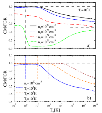
Figure 5: (Color online) Ratio of the CM and FGR energy transfer rates for fully ionized hydrogen as a function of the electron temperature. Panel a) considers various densities while the ion temperature is constant; panel b) shows results for different ion temperatures at constant density. All results are obtained within the random phase approximation. The vertical lines mark the condition $T_{e}\!=\!T_{i}$.

Of course, an increasing ion temperature has a similar effect as a decreasing electron density as shown in the second panel of Fig. 5 where the well established CM effect for $T_{i}=10^{4}K$ vanishes for higher ion temperatures. Nevertheless, sufficiently high electron temperatures always guarantee that the CM rates are lower than FGR or LS rates in these parameter regions.

Interestingly, the ratio of the CM and FGR rates seems to always approach 1/2 in the limit of high electron temperatures. In laser-produced plasmas with $T_{e}\!\gg\!T_{i}$, one should therefore almost always expect reduced energy transfer rates due to coupled collective modes. On the other hand, the density in a shock-produced plasma ($T_{e}\!<\!T_{i}$) must be high enough to observe CM effects.

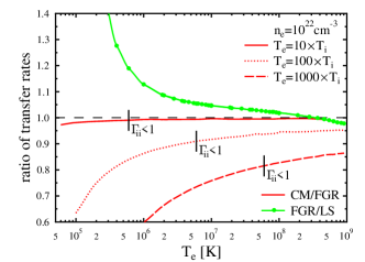
Figure 6: (Color online) Ratio of energy transfer rates in CM, FGR, and LS in the high temperature (low coupling) limit for fully ionized hydrogen. Curves for different ratios of electron and ion temperature are given. The three curves below unity belong to the ratio of CM to FGR rate. The ratio of FGR rate and LS rate is independent of the temperature ratio and is given by the green dotted line. The region were the ion coupling is small is indicated for each case.

Let us analyze the above mentioned high temperature, low density limit of the CM energy transfer rate in more detail (see Fig. 6). The CM and FGR approaches do agree in the weak coupling limit if and only if the temperature difference between the subsystems is sufficiently low so that no coupled collective modes can be excited. Larger deviations occur for increased temperature differences and smaller electron temperatures (more strongly coupled ions; although RPA is used in Fig. 6). However, even for very large electron temperatures the CM effects still reduce the coupling between the electron and ion components.

Moreover, FGR and LS have a ratio independent of the temperature difference. In addition, numerics show, that even in the weakly coupled case with small temperature difference, FGR and LS curves intersect rather than converge. This is due to the poor cut off in the Coulomb integral in LS. Thus the FGR approach rather than LS formula should be used to compare with experiments or simulations if one searches for coupled mode effects in the data.

Of particular interest is the question whether the easier FGR is strictly valid in some cases or not. The difference between FGR and CM originates from the different denominators. Within RPA, one easily obtains

$$|\varepsilon^{R}(k,\omega)|^{2}\!\! = \!\!|\varepsilon_{ee}(k,\omega)|^{2}\,|\varepsilon_{ii}(k,\omega)|^{2}$$ (14)

$$+2V_{ee}(k)V_{ii}(k)\,\mathop{\mathrm{Re}}\chi^{0}_{ee}(k,\omega)\mathop{\mathrm{Re}}\chi^{0}_{ii}(k,\omega)$$

$$+2V_{ee}(k)V_{ii}(k)\,\mathop{\mathrm{Im}}\chi^{0}_{ee}(k,\omega)\mathop{\mathrm{Im}}\chi^{0}_{ii}(k,\omega)$$

$$-\Big{[}|\varepsilon_{ee}(k,\omega)|^{2}-1\Big{]}\Big{[}|\varepsilon_{ii}(k,\omega)|^{2}-1\Big{]}\,.$$

For the FGR approach to be accurate, the first line only most hold. Strictly, this is only possible for very large wave numbers $k$. For the interesting small $k$ values, we must require low plasma densities and the static case with vanishing imaginary contributions. However, it is essential for the occurrence of coupled collective modes and the resulting mechanism of energy transfer to retain the frequency dependence in the dielectric functions. Whenever, the FGR and CM modes agree (numerics shows us that this requires the non-occurance of ion acoustic modes), it results from redistributing weights and is a numerical and approximate agreement of the expressions.

IV.2 Charge State and Strong Coupling Effects

Coupled mode effects on the energy transfer rates are of course much more pronounced for plasma ions with higher charges since here the ion acoustic modes occur for smaller temperature differences or even $T_{e}\!=\!T_{i}$ (see Eq. (9). These modes exist also for higher $k$ values if the ion charge is higher. Different masses of the ions also shift the modes to different locations in $k$ space which is, however, irrelevant for the (relative) CM effect as the modes in FGR behave similarly.

In addition to the charge state, strong coupling effects must be investigated as the CM reduction of the rates is stronger for colder system as shown in Fig. 6. In this case, the ions can be strongly coupled and not described within RPA. Thus, both strong coupling and collective excitations must be considered in many situations.

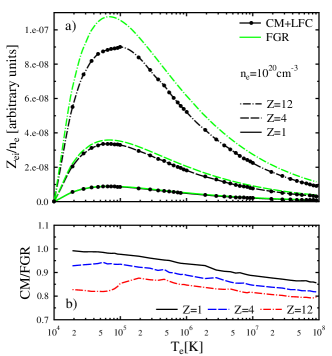
Figure 7: (Color online) Effect of the (nonequilibrium) ion charge state on the energy transfer rates in different approximations for a high–Z plasma. Panel a) displays the rates and panel b) shows the ratio of the CM and FGR results. The ion temperature is $T_{i}=10^{4}K$.

Figure 7 shows an example for plasmas with highly charged ions. When normalized to the electron density the energy transfer rates rise linearly with the charge $Z$ in the FGR and LS approaches. CM energy transfer rates naturally depend stronger on the coupled mode structure. Panel b) of Fig. 7 shows that the relative reduction for $Z=4$ is higher than for $Z=1$ so that the charge dependence of CM rates is smaller than $Z$. We find charge state effects especially for smaller electron temperatures where the occurance of the ion acoustic mode strongly depends on the charge state of the ion (see in Eqs. (9)). If the electron temperature is already high enough to allow for the mode at $Z\!=\!1$, the charge state effect is much weaker. For the highest charge state considered in Fig. 7, the influence of the CM rates is even more strongly pronounced due to strong coupling effects.

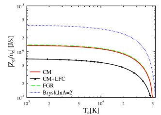
Figure 8: (Color online) Energy transfer rate for shocked silicon at $n_{e}\!=\!5.36\times 10^{23}\,$cm^-3, $T_{i}\!=\!54539\,$K, and with $Z\!=\!4$ in different approximations. The electron Fermi temperature is $T_{F}\!=\!2.8\times 10^{5}\,$K. These conditions are as in the experiment of Ng et al. NCXF_95 .

The second example in Fig. 8 considers the situation in shocked silicon plasmas as prepared in the experiment by Ng et al. NCXF_95 . For this case, the electron temperature is lower than the ion temperature. The electrons are highly degenerate so that according to Eq. (9) CM effects are possible since the Fermi temperature considerably exceeds the ion temperature. The ions are also strongly coupled, $\Gamma_{ii}\!=\!64$, and local field corrections to the response functions have a larger effect as in the examples given so far.

When analysing the case, the first point to realise is that neither the usual Landau-Spitzer approach nor the Brysk formula B_74 that (partially) accounts for degeneracy effects is well defined. Both formulas contain a Coulomb logarithm that either becomes negative or very small when considering straight line trajectories or hyperbolic orbits, respectively. Thus, the Coulomb logarithm is usually clamped at some larger value. Here, we use $\lambda_{C}\!=\!2$ for comparison. Still both the LS and Brysk formula give energy transfer rates that are orders of magnitude larger than the FGR or CM results which acount for degenerate electrons in a regular fashion. This is qualitatively consistent with the experimentally observed facts.

Comparing the rates obtained by the CM and FGR expressions, one makes an interesting observation: on the RPA level both approaches yield more or less the same results although ion acoustic modes are present in the system. The weighting due to the electron Fermi distributions favors however larger $k$ values where no collective mode exist. However, we find a further reduction of the CM rates when the effect of strong coupling is included by static local field corrections. Since the FGR approach naturally includes strong coupling effect HZRD_01 , no changes occur within this approach. Accordingly, we find now a factor of roughly two between the rates calculated by the CM and FGR expressions, respectively. Thus, we can confirm the occurance of coupled mode effects under these conditions although the main effect arises from the correct treatment of degeneracy.

V Conclusions

We investigated the electron-ion energy transfer rates in two-temperature plasmas with special emphasis on coupled mode effects. For weakly coupled plasmas, the starting point was the quantum version of the Lennard-Balescu kinetic equation which naturally includes fully coupled collective excitations in the screening function. It was shown that a straightforward derivation without further approximations yields a coupled mode expression for the energy relaxation rates. This kinetic approach is consistent and accurate for weakly coupled plasmas of any degeneracy. It can be easily extended to plasmas with strongly coupled ions by including (static) local field corrections.

For certain conditions, the coupled mode expression yield considerably reduced electron-ion energy transfers when compared to the LS and FGR approaches. A detailed analysis showed that this reduction can be traced back to the occurance of ion acoustic modes and a related redistribution of weight in the dielectric response function. This reflects the fact that the coupled mode approach consideres a much more realistic mode structure. Precise conditions for the occurrence of ion accoustic modes and the coupled mode reduction of the energy transfer rates were derived. Interestingly, the CM reduction is preserved for very high electron temperatures where the rates are roughly a factor of two less than the ones calculated with the FGR or LS approaches. An agreement between CM and FGR expressions can only be reached if the temperature difference is small or the ion temperature is high enough to prohibit the occurance of ion acoustic modes.

The results presented here are concistent with experimental RWSW_00 ; CNXF_92 ; NCXF_95 and theoretical DP_98 ; D_01 findings of lowered electron-ion energy transfers and thus longer equilibration times. In particular, the strong reduction of the equilibration rates in shocked silicon is in qualitative agreement with measurements. The experiments probed however regimes where collective modes as well as strong binary collisions and changing potential energies are of importance. Thus, a full description must also include these effects at least on a level as described in Refs. GMS_02 ; GM_05 ; G_05 . The conditions for the occurance of CM effects derived also explain why no or very small CM reductions have been seen in recent numerical simulations GGMM_08 ; DD_08 ; JFCC_08 .

Appendix A Derivation Coupled Mode Expression in Random Phase Approximation

We start with the quantum Lennard-Balescu equation for the electron distribution $f_{e}(p,t)$ in homogeneous and isotropic plasmas brown

$$\frac{\partial}{\partial t}f_{e}(p,t) \!\!=\!\! \frac{1}{\hbar}\sum\limits_{i}\int\frac{d{\mbox{\boldmath$p$}}^{\prime}}{{(2\pi\hbar)^{3}}}\frac{d{\mbox{\boldmath$\overline{p}$}}}{{(2\pi\hbar)^{3}}}\frac{d{\mbox{\boldmath$\overline{p}$}}^{\prime}}{{(2\pi\hbar)^{3}}}\,\left|\frac{{\mathrm{V}}_{ei}({\mbox{\boldmath$p$}}-{\mbox{\boldmath$\overline{p}$}})}{\varepsilon^{RPA}\left({\mbox{\boldmath$p$}}-{\mbox{\boldmath$\overline{p}$}},E_{e}(p)-E_{e}({\overline{p}}),t\right)}\right|^{2}$$

$$\times 2\pi\delta\!\;\Big{(}E_{e}({\mbox{\boldmath$p$}})+E_{i}({\mbox{\boldmath$p$}}^{\prime})-E_{e}({\mbox{\boldmath$\overline{p}$}})-E_{i}({\mbox{\boldmath$\overline{p}$}}^{\prime})\Big{)}\;{(2\pi\hbar)^{3}}\,\delta\!\!\;\Big{(}{\mbox{\boldmath$p$}}+{\mbox{\boldmath$p$}}^{\prime}-{\mbox{\boldmath$\overline{p}$}}-{\mbox{\boldmath$\overline{p}$}}^{\prime}\Big{)}$$

$$\times\Big{\{}f_{e}({\mbox{\boldmath$\overline{p}$}},t)f_{i}({\mbox{\boldmath$\overline{p}$}}^{\prime},t)\,[1-f_{e}({\mbox{\boldmath$p$}},t)]\,[1-f_{i}({\mbox{\boldmath$p$}}^{\prime},t)]-f_{e}({\mbox{\boldmath$p$}},t)f_{i}({\mbox{\boldmath$p$}}^{\prime},t)\,[1-f_{e}({\mbox{\boldmath$\overline{p}$}},t)]\,[1-f_{i}({\mbox{\boldmath$\overline{p}$}}^{\prime},t)]\Big{\}}\,.$$

The sum runs over all species, but only the ions contribute to the energy relaxation. $E_{a}(p)\!=\!p^{2}/2m_{a}$ denotes the kinetic energy of particles of species $a$ and $V_{ab}(k)\!=\!4\pi Z_{a}Z_{b}e^{2}/k^{2}$ the (unscreened) Coulomb potential. Dynamic screening is described by the retarded dielectric function which is used here in RPA

$$\varepsilon^{RPA}({\mbox{\boldmath$p$}},E,t) = 1-\sum_{a}\;V_{aa}(p)\,\chi^{0}_{aa}({\mbox{\boldmath$p$}},E,t)\,.$$ (16)

The upper expression relates the screening function to the density response function of free particles given by

$$\chi^{0}_{aa}({\mbox{\boldmath$p$}},E,t)=\int\frac{d{\mbox{\boldmath$p$}}^{\prime}}{{(2\pi\hbar)^{3}}}\frac{f_{a}({\mbox{\boldmath$p$}}^{\prime},t)-f_{a}({\mbox{\boldmath$p$}}^{\prime}+{\mbox{\boldmath$p$}},t)}{E+E_{a}({\mbox{\boldmath$p$}}^{\prime})-E_{a}({\mbox{\boldmath$p$}}^{\prime}+{\mbox{\boldmath$p$}})+i\epsilon}\,,$$ (17)

which is, in turn, determined by the electron or the ion distribution function.

The electron-ion energy transfer rates are now obtained by multiplying the Lenard-Balescu equation (LABEL:balescu_gl) by the electron energy, $E_{e}=p^{2}/2m_{e}$, and an integration over the free momentum (see balance equation (1).

For the further proceedings, it is useful to use the momentum and the energy transfer during the collision, ${\mbox{\boldmath$k$}}\!=\!{\mbox{\boldmath$p$}}\!-\!{\mbox{\boldmath$\overline{p}$}}$ and $\omega\!=\!E_{e}(p)\!-\!E_{e}({\overline{p}})$, respectively. With these new variables, one can now apply the relations between Fermi-distributions of the plasma species and Bose functions $n_{B}^{a}(\omega)\!=\![\exp(\hbar\omega/k_{B}T_{a})\!-\!1]^{-1}$, namely

$$\!\!\!\!\!f_{a}({\mbox{\boldmath$p$}})\,[1-f_{a}({\mbox{\boldmath$p$}}+{\mbox{\boldmath$k$}})]=$$ (18)

$$[f_{a}({\mbox{\boldmath$p$}}+{\mbox{\boldmath$k$}})-f_{a}({\mbox{\boldmath$p$}})]\,n_{B}^{a}\!\Big{(}E_{a}({\mbox{\boldmath$p$}})-E_{a}({\mbox{\boldmath$p$}}+{\mbox{\boldmath$k$}})\Big{)}\,,$$

$$\!\!\!\!\!f_{a}({\mbox{\boldmath$p$}}+{\mbox{\boldmath$k$}})\,[1-f_{a}({\mbox{\boldmath$p$}})]=$$ (19)

$$[f_{a}({\mbox{\boldmath$p$}})-f_{a}({\mbox{\boldmath$p$}}+{\mbox{\boldmath$k$}})]n_{B}^{a}\!\Big{(}E_{a}({\mbox{\boldmath$p$}}+{\mbox{\boldmath$k$}})-E_{a}({\mbox{\boldmath$p$}})\Big{)}\,.$$

The set of distributions in the third line of the collision integral of the Lenard-Balescu equation (LABEL:balescu_gl) can then be written as

$$\Big{\{}f()\Big{\}}\!\! = \!\![f_{e}({\mbox{\boldmath$\overline{p}$}}+{\mbox{\boldmath$k$}})-f_{e}({\mbox{\boldmath$\overline{p}$}})]\,[f_{i}({\mbox{\boldmath$p$}}^{\prime})-f_{i}({\mbox{\boldmath$p$}}^{\prime}+{\mbox{\boldmath$k$}})]$$ (20)

$$\!\!\times\Big{[}n_{B}^{e}(-\omega)\,n_{B}^{i}(\omega)-n_{B}^{e}(\omega)\,n_{B}^{i}(-\omega)\Big{]}\,.$$

With these transformations, we obtain for the electron-ion energy transfer rate

$$\frac{\partial}{\partial t}E^{CM}_{e\to i} \!\!=\!\! -\frac{1}{\hbar}\sum\limits_{i}\int\frac{d{\mbox{\boldmath$\overline{p}$}}}{{(2\pi\hbar)^{3}}}\frac{d{\mbox{\boldmath$k$}}}{{(2\pi\hbar)^{3}}}\frac{d\omega}{2\pi}\;E_{e}({\mbox{\boldmath$\overline{p}$}}+{\mbox{\boldmath$k$}})\;\left|\frac{{\mathrm{V}}_{ei}({\mbox{\boldmath$k$}})}{\varepsilon^{R}({\mbox{\boldmath$k$}}\omega)}\right|^{2}\Big{[}f_{e}({\mbox{\boldmath$\overline{p}$}}+{\mbox{\boldmath$k$}})-f_{e}({\mbox{\boldmath$\overline{p}$}})\Big{]}2\pi\delta\!\!\;\Big{(}\omega-E_{e}({\mbox{\boldmath$\overline{p}$}}+{\mbox{\boldmath$k$}})+E_{e}({\mbox{\boldmath$\overline{p}$}})\Big{)}$$

$$\times\Big{[}n_{B}^{e}(-\omega)\,n_{B}^{i}(\omega)-n_{B}^{e}(\omega)\,n_{B}^{i}(-\omega)\Big{]}\;\int\frac{d{\mbox{\boldmath$p$}}^{\prime}}{{(2\pi\hbar)^{3}}}\>[f_{i}({\mbox{\boldmath$p$}}^{\prime})-f_{i}({\mbox{\boldmath$p$}}^{\prime}+{\mbox{\boldmath$k$}})]\>\,2\pi\delta\!\!\;\Big{(}\omega-E_{i}({\mbox{\boldmath$p$}}^{\prime}+{\mbox{\boldmath$k$}})+E_{i}({\mbox{\boldmath$\overline{p}$}}^{\prime})\Big{)}\,.$$

The integral in the second line of this expression is just the definition of the imaginary part of the free particle density response function for the ionic subsystem $\mathop{\mathrm{Im}}\chi^{0}_{ii}(k\omega)$ as defined by (17). The difference of Bose functions in the second line determines the direction of the energy transfer. After another variable transformation to $\omega^{\prime}\!=\!-\omega$, ${\mbox{\boldmath$k$}}^{\prime}\!=\!-{\mbox{\boldmath$k$}}$, and ${\mbox{\boldmath$p$}}^{\prime}\!=\!{\mbox{\boldmath$\overline{p}$}}\!-\!{\mbox{\boldmath$k$}}^{\prime}$ (changing the sign) in the second term proportional to $n_{B}^{e}(\omega)\,n_{B}^{i}(-\omega)$, this second term has the same form as the first one, except that the energy in front of the screened potential is $E_{e}({\mbox{\boldmath$\overline{p}$}})$ instead of $E_{e}({\mbox{\boldmath$\overline{p}$}}\!-\!{\mbox{\boldmath$k$}})$. Applying the energy conserving $\delta$-function in the collision integral yields

$$E_{e}({\mbox{\boldmath$\overline{p}$}}+{\mbox{\boldmath$k$}})-E_{e}({\mbox{\boldmath$\overline{p}$}})=\omega\,.$$ (22)

Now the remaining electron distributions together with the energy conserving $\delta$-function give also the definition of an imaginary part of the free density response function; this time, the one for the electrons, i.e. $\mathop{\mathrm{Im}}\chi^{0}_{ee}(k\omega)$. The energy transfer rate is thus given by

$$\frac{\partial}{\partial t}E^{CM}_{e\to i} \!\!=\!\! -4\hbar\sum\limits_{i}\int\frac{d{\mbox{\boldmath$k$}}}{{(2\pi\hbar)^{3}}}\int\limits_{-\infty}^{\infty}\!\!\frac{d\omega}{2\pi}\,\omega\,\left|\frac{{\mathrm{V}}_{ei}(k)}{\varepsilon^{RPA}(k\omega)}\right|^{2}\;$$

$$\times\mathop{\mathrm{Im}}\chi^{0}_{ee}(k\omega)\,\mathop{\mathrm{Im}}\chi^{0}_{ii}(k\omega)\,n_{B}^{e}(-\omega)\,n_{B}^{i}(\omega)\,.$$

If we use the fact that $[1/2\!-\!n_{B}(\omega)]$ and $\mathop{\mathrm{Im}}\chi^{0}_{aa}(\omega)$ are odd functions with respect to $\omega$, we can rearrange the upper expression in the form

$$\frac{\partial}{\partial t}E^{CM}_{e\to i} \!\!=\!\! -4\hbar\sum\limits_{i}\int\frac{d{\mbox{\boldmath$k$}}}{{(2\pi\hbar)^{3}}}\int\limits_{0}^{\infty}\!\!\frac{d\omega}{2\pi}\;\>\omega\,\left|\frac{{\mathrm{V}}_{ei}(k)}{\varepsilon^{RPA}(k\omega)}\right|^{2}\;$$

$$\times\mathop{\mathrm{Im}}\chi^{0}_{ee}(k\omega)\,\mathop{\mathrm{Im}}\chi^{0}_{ii}(k\omega)\,\Big{[}n_{B}^{e}(\omega)-n_{B}^{i}(\omega)\Big{]}\,.$$

This expression gives the electron-ion energy transfer rate including the effects of fully coupled collective modes in the electron-ion system. Similar to the Lenard-Balescu equation that was used as a starting point, it describes weakly coupled plasmas without restriction with respect to the degeneracy.

Appendix B Equivalence to Coupled Mode Description by Dharma-wardana & Perrot

The coupled mode expression derived by Dharma-wardana & Perrot, equation (50) in Ref. DP_98 , reads

$$\dot{E}_{rlx} \!\!=\!\! \hbar\int\limits_{0}^{\infty}\frac{d\omega}{2\pi}\int\frac{d{\bf k}}{(2\pi\hbar)^{3}}\;\omega\,V_{ie}^{2}(k)$$ (25)

$$\times\frac{\Delta N_{ei}(\omega)\,A^{i}(k,\omega)\,A^{e}(k,\omega)}{|1-V_{ie}^{2}(k)\,\chi_{ee}(k,\omega)\,\chi_{ii}(k,\omega)|^{2}}\,,$$

where we assumed all potentials to be of Coulomb type for simplicity. The difference of Bose functions is here the same as in Eq. (LABEL:coupled_transf_a_appen): $\Delta N_{ei}\!=\!n_{B}^{e}(\omega)-n_{B}^{i}(\omega)$. The functions $A^{a}(k,\omega)$ are related to the imaginary parts of the response functions $\chi_{aa}(k,\omega)$

$$A^{a}(k,\omega)=-2\mbox{Im}\chi_{aa}(k,\omega)\,.$$ (26)

One should however notice that these are full density response functions of a coupled system.

The density response function $\chi_{aa}$ for a single species can also be written in terms of the polarization function $\Pi_{aa}$ and the dielectric function $\varepsilon$ of the (fully coupled) medium. Neglecting cross terms, we have green

$$\chi_{aa}(k,\omega)=\frac{\Pi_{aa}(k,\omega)}{1-V_{aa}(k)\Pi_{aa}(k,\omega)}=\frac{\Pi_{aa}(k,\omega)}{\varepsilon_{aa}(k,\omega)}\,.$$ (27)

This is nothing else than the equation of motion for the density response function. Real and imaginary parts of the response function can then be expressed as

$$\mbox{Re}\chi_{aa}(k,\omega) \!\!=\!\! \frac{\mbox{Re}\varepsilon_{a}(k,\omega)-|\varepsilon_{a}(k,\omega)|^{2}}{V_{aa}(k)|\varepsilon_{a}(k,\omega)|^{2}}\,,$$ (28)

$$\mbox{Im}\chi_{aa}(k,\omega) \!\!=\!\! -\frac{\mbox{Im}\varepsilon_{a}(k,\omega)}{V_{aa}(k)|\varepsilon_{a}(k,\omega)|^{2}}\,.$$ (29)

With the help of these expressions, the denominator in expression (25) which constitudes the differences to the FGR formula becomes

$$|1-V_{ie}^{2}(k)\,\chi_{ee}(k,\omega)\chi_{ii}(k,\omega)|^{2}$$ (30)

$$\qquad\qquad\qquad=\frac{|\varepsilon(k,\omega)|^{2}}{|\varepsilon_{e}(k,\omega)|^{2}|\varepsilon_{i}(k,\omega)|^{2}}\,.$$

The dielectric function in the numerator of Eq. (30) is the one for the full system given by $\varepsilon=1-\sum_{a}V_{aa}\Pi_{aa}$. The partial dielectric functions $\varepsilon_{a}$ in this expression are cancled by the one contained in the imaginary part of the full density response function $\chi_{aa}$ when the latter are written as in eq. (29). Accordingly, one obtains an expression identical to Eq. (LABEL:coupled_transf_a_appen) when inserting these definitions and transformations into Eq. (25).

Appendix C Conditions for the Occurance of Ion Acoustic Modes

It is well known that ion accoustic modes occur in non-equilibrium plasmas with $T_{e}\!\gg\!T_{i}$ LL_81 . Here, we give a more precise estimate of the necessary temperature relation needed to allow for this type of collective modes in weakly coupled plasmas.

For ion acoustic modes to exist, the real part of the total dielectric function must vanish. We first consider the ionic contribution in non-degenerate limit which is almost always sufficient for the heavy ions. In RPA, the polarisation function is identical to the free particle density response function, that is $\Pi_{ii}\!=\!\chi_{ii}^{0}$. Its real part can be written in terms of the confluent hypergeometric function green ; brown

$$\mbox{Re}\chi^{0}_{ii}(k,\omega)=\frac{n_{i}}{k_{B}T}\left[1-\frac{\omega^{2}m_{i}}{p^{2}k_{B}T}\,_{1}F_{1}\!\left(1,\frac{3}{2},-\frac{\omega^{2}m_{i}}{2p^{2}k_{B}T}\right)\right]$$ (31)

which is defined over an integral grad . However, one can approximate this function for the special first two arguments needed by the following Padé formula brown

$${}_{1}F_{1}\!\left(1,\frac{3}{2},-x\right)=$$ (32)

$$\frac{1+\frac{x}{3}+\frac{x^{2}}{10}+\frac{x^{3}}{42}+\frac{x^{4}}{218}+\frac{7x^{5}+x^{6}}{9360}}{1+x+\frac{x^{2}}{2}+\frac{x^{3}}{6}+\frac{x^{4}}{24}+\frac{x^{5}}{120}+\frac{x^{6}}{720}+\frac{x^{7}}{4860}}\,.$$

As a required condition for ion acoustic modes to occur, the minimum of the response functions (31) must at least compensate the electronic contribution plus unity. We thus search for an approximation of Eq. (32) that conserves this minimum. Performing a frequency derivative, we find its location to be approximately at $\omega_{0}\!=\!2.36\,k\,(k_{B}T_{i}/m_{i})^{1/2}$. Using the minimum frequency $\omega_{0}$ in Eq. (31) with the hypergeometric function given by Eq. (32) yields

$$\mbox{Re}\;\!\varepsilon_{i}(k,\omega_{0})=1-0.27\,\frac{\kappa_{i}^{2}}{k^{2}}\,,$$ (33)

where $\kappa_{i}=(4\pi Z_{i}^{2}e^{2}n_{i}/k_{B}T_{i})^{1/2}$ is the inverse of the ion part of the classical Debye screening length.

The electronic part of the dielectric function can be very well estimated in the zero frequency (static) long wave length limit

$$\mbox{Re}\;\!\varepsilon_{e}(k,0)=1+\frac{\kappa_{e}^{2}}{k^{2}}\,.$$ (34)

Again, $\kappa$ denotes the inverse screening length. For small momenta, the unity in Eqs. (33) and (34) can be neglected. The condition for the ion acoustic modes to emerge becomes then

$$\kappa_{e}^{2}\leq 0.27\,\kappa_{i}^{2}\,.$$ (35)

Eq. (35) quantifies the long known condition of $T_{i}\ll T_{e}$ LL_81 for the ion acoustic waves to occur. Direct relations for the electron and ion temperatures needed may be obtained by inserting an appropriate expression for the electron screening length. In the nondegenerate limit, it is given by the electron Debye length and one obtains the upper relation of Eq. (9). For highly degenerate electrons, Thomas-Fermi screening with $\kappa_{e}\!=\!\kappa_{TF}^{2}\!=\!4m_{e}e^{2}(3n_{e}/\pi)^{1/3}$ must be used. Since the Thomas-Fermi length is temperature independent, the role of the electron temperature is taken over by the electron Fermi temperature which yields the second condition in Eq. (9) for the existence of the ion acoustic modes. Accordingly, they can also occur in degenerate plasmas at equilibrium or even in shock-produced high-density plasmas with $T_{e}\!<\!T_{i}$.

References

- (1) G.W. Collins at al., Science 281, 1178 (1998).
- (2) M.D. Knudson, D.L. Hanson, J.E. Bailey, C.A. Hall, and J.R. Asay, and W.W. Anderson, Phys. Rev. Lett. 87, 225501 (2001).
-
(3)
D. Riley, N.C. Woolsey, D. McSherry, I. Weaver,
A. Djaoui, and E. Nardi, Phys. Rev. Lett. 84, 1704 (2000). - (4) A. Ravasio et al., Phys. Rev. Lett. 99, 135006 (2007).
- (5) S.H. Glenzer et al., Phys. Rev. Lett. 98, 065002 (2007).
- (6) E. Garćia Saiz at el., accepted for publication in Nature Physics.
- (7) A.L. Kritcher at al., Science 322, 69 (2008).
- (8) P. Celliers, A. Ng, G. Xu, and A. Forsman, Phys. Rev. Lett. 68, 2305 (1992).
- (9) A. Ng, P. Celliers, G. Xu, and A. Forsman, Phys. Rev. E 52, 4299 (1995).
- (10) D.O. Gericke, M.S. Murillo, and M. Schlanges, Phys. Rev. E 65, 036418 (2002).
- (11) D.O. Gericke, M.S. Murillo, and M. Schlanges, Laser and Part. Beams 20, 543 (2002).
- (12) The break-down of the classical collision theory first yields too low than negative Coulomb logarithms which translates into too low or negative energy transfer rates in the Landau-Spitzer theory.
-
(13)
G. Hazak, Z. Zinamon, Y. Rosenfeld, and
M.W.C. Dharma-wardana, Phys. Rev. E 64, 066411 (2001). - (14) D.O. Gericke and M.S. Murillo, Proceedings Int. Conf. on Inertial Fusion Science and Applications , edited by W.J. Hogan, Monterey (2004).
- (15) D.O. Gericke, M.S. Murillo, D. Semkat, M. Bonitz, and D. Kremp, J. Phys. A 36, 6087 (2003).
- (16) D.O. Gericke, Th. Bornath, and M. Schlanges, J. Phys. A 39, 4739 (2006).
- (17) Th. Ohde, M. Bonitz, Th. Bornath, D. Kremp, and M. Schlanges, Phys. Plasmas 3, 1241 (1996).
- (18) Th. Bornath, M. Schlanges, and R. Prenzel, Phys. Plasmas 5, 1485 (1998).
-
(19)
D.O. Gericke, G.K. Grubert, Th. Bornath, and
M. Schlanges, J. Phys. A 39, 4727 (2006). - (20) M.W.C. Dharma-wardana and F. Perrot, Phys. Rev. E 58, 3705 (1998).
- (21) M.W.C. Dharma-wardana, Phys. Rev. E 64, 035401(R) (2001).
- (22) J. Daligault and D. Mozyrsky, Phys. Rev. E 75, 026402 (2007).
- (23) J. Daligault and D. Mozyrsky, High Energy Density Physics 4, 58 (2008).
- (24) G. Gregori and D.O. Gericke, Europhys. Lett. 83, 15002 (2008).
- (25) A. Lenard, Ann. Phys. 3, 390 (1960).
- (26) R. Balescu, Phys. Fluids 3, 52 (1960).
- (27) D. Kremp, M. Schlanges, and W.-D. Kraeft, Quantum Statistics of Nonideal Plasmas (Springer, Berlin, 2006).
- (28) J.N. Glosli et al., Phys. Rev. E 78, 025401(R) (2008).
- (29) B. Jeon, M. Foster, J. Colgan, G. Csanak, J.D. Kress, L.A. Collins, and N. Grønbech-Jensen, Phys. Rev. E 78, 036403 (2008).
- (30) L.D. Landau, Phys. Z. Sowjetunion 10 154 (1936).
- (31) P. Danielewicz, Ann. Phys. (N.Y.) 152 239 (1984).
- (32) L. Spitzer, Physics of Fully Ionized Gases (Interscience, New York, 1962).
- (33) D.O. Gericke, J. Phys. (Conf. Series) 11, 111 (2005).
- (34) V.M. Zhdanov, Transport Processes in Multicomponent Plasma (Taylor & Francis, London, New York, 2002).
- (35) S. Ichimaru, Rev. Mod. Phys. 54, 1017 (1982).
- (36) J.P. Hansen and I.R. McDonald, Theory of Simple Liquids (Academic Press, London, 1990).
-
(37)
L.D. Landau and E.M. Lifshitz,
Course in Theoretical
Physics (Pergamon, Oxford, 1981). - (38) G. Dimonte and J. Daligault, Phys. Rev. Lett. 101, 135001 (2008).
- (39) J. Vorberger, D.O. Gericke, J. Phys. (Conf. Series) 112, 032077 (2008).
- (40) W.-D. Kraeft, B. Strege, and M. Girardeau, Contrib. Plasma Phys. 30, 563 (1990).
- (41) H. Brysk, Plasma Phys. 16, 927 (1974).
-
(42)
W.-D. Kraeft, D. Kremp, W. Ebeling, and G. Röpke,
Quantum Statistics of Charged Particle Systems
(Akademie-Verlag, Berlin, 1986). -
(43)
I.S. Gradshteyn and I.M. Ryzhik,
Table of Integrals,
Series, and Products (Academic Press, San Diego, 1980).