Intermode Dephasing in a Superconducting Stripline Resonator - Supplementary Information

This paper contains suplementary information for Suchoi et al. (2009). The supplementary information is devoted to three main issues. In section I we describe the fabrication process; in section II we present the derivation of the Hamiltonian of the system and provide a more detailed discussion about the properties of the microbridges; in section III the hysteretic response of the resonator and the effect of heating are discussed.

I Fabrication processes

The fabrication process starts with a high resistivity Si substrate coated with SiN layers of thickness $100\operatorname{nm}$ on both sides. A $150\operatorname{nm}$ thick Nb layer is deposited on the wafer using magnetron DC sputtering. Then, e-beam lithography and a subsequent liftoff process are employed to pattern an Al mask, which defines the SSR and the SQUID leads. The device is then etched using electron cyclotron resonance system with CF₄ plasma. The nanobridges are fabricated using FEI Strata 400 Focus Ion Beam (FIB) system Hao et al. (2008, 2007); Bell et al. (2003); Datesman et al. (2005a); Troeman et al. (2007) at accelerating voltage of $30\operatorname{kV}$ and Ga ions current of $9.7$ pA. The outer dimensions of the bridges are about $150\times 50\operatorname{nm}.$ However, the actual dimensions of the weak-links are smaller, since the bombarding Ga ions penetrate into the Nb layer, and consequently, suppress superconductivity over a depth estimated between $30\operatorname{nm}$ to $50\operatorname{nm}$ Troeman et al. (2007); Datesman et al. (2005b).

II Detailed derivation of the effective Hamiltonian

The effective Hamiltonian of the closed system comprising the SSR and the SQUID Clark et al. (2001); Blencowe and Buks (2007) is found using the same method that was previously employed in Refs. Blencowe and Buks (2007); Nation et al. (2008). Here however, we relax the assumption that the self inductance of the SQUID loop is small, and also the assumption that both junctions have the same critical currents. On the other hand, we assume that the inductance of the SQUID, which is denoted as $L_{\mathrm{S}}$, is much smaller than the total inductance of the stripline $L_{\mathrm{T}}l_{\mathrm{T}}$. This assumption can be justified by considering the fact that the measured angular resonance frequencies $\omega_{n}$ of the first 3 modes ($n\in\left\{1,2,3\right\}$) for all values of $\Phi_{x}$ (see Figs. 2 and 3 in Suchoi et al. (2009)) are very close to the values expected from a uniform resonator having length $l_{\mathrm{T}}$, namely $n\omega_{\mathrm{T}}$, where $\omega_{\mathrm{T}}=\pi/l_{\mathrm{T}}\sqrt{L_{\mathrm{T}}C_{\mathrm{T}}}$. Moreover, the normalized flux-induced shift $\Delta\omega_{n}/n\omega_{\mathrm{T}}$ in the angular resonance frequency of the first 3 modes is quite small and never exceeds $10^{-3}$. Both observations indicate that the ratio $L_{\mathrm{S}}/L_{\mathrm{T}}l_{\mathrm{T}}$ can indeed be considered as a small parameter.

The resultant Hamiltonian of the closed system is given by $\mathcal{H}=\mathcal{H}_{\mathrm{SSR}}+\mathcal{H}_{\mathrm{S}}\left(I\right)$, where $\mathcal{H}_{\mathrm{SSR}}$ is the SSR Hamiltonian and where $\mathcal{H}_{\mathrm{S}}\left(I\right)$ is the SQUID Hamiltonian, which depends on the current $I$ at the center of the SSR, namely, the current flowing through the SQUID. In terms of annihilation ($A_{1}$ and $A_{3}$) and creation ($A_{1}^{{\dagger}}$ and $A_{3}^{{\dagger}}$) operators for the first and third modes of the SSR respectively, the Hamiltonian $\mathcal{H}_{\mathrm{SSR}}$ can be expressed as

$$\mathcal{H}_{\mathrm{SSR}}=\hbar\omega_{\mathrm{T}}\left(N_{1}+3N_{3}\right)+V_{\mathrm{in}}\;,$$ (1)

where $N_{1}=A_{1}^{{\dagger}}A_{1}$ and $N_{3}=A_{3}^{{\dagger}}A_{3}$ are number operators,

$$V_{\mathrm{in}}=\hbar\sqrt{2\gamma_{\mathrm{f}1}}b_{1}^{\mathrm{in}}\left(e^{-i\omega_{\mathrm{p}}t}A_{1}+e^{i\omega_{\mathrm{p}}t}A_{1}^{{\dagger}}\right)$$ (2)

represents the external driving, $\gamma_{\mathrm{f}1}$ is the coupling constant between the 1st mode and the feedline, $b_{1}^{\mathrm{in}}$ is the amplitude of the driving pump tone, which is injected into the feedline to excite the first mode, and $\omega_{\mathrm{p}}$ is its angular frequency.

II.1 The kinetic inductance of the nanobridges

The Hamiltonian for the SQUID depends on the properties of the nanobridges. Due to the Ga ions implanted in the outer layer of the Niobium during the FIB process and the consequent suppression of superconductivity in that layer Troeman et al. (2007); Datesman et al. (2005b), the weak links are treated as variable thickness nanobridges. The behavior of such a nanobridge is strongly dependent on the ratio $l/\xi$ Granata et al. (2008); Hasselbach et al. (2002, 2000); Baratoff et al. (1970); Likharev (1979); Likharev and Yakobson (1975); Gumann et al. (2007); Podd et al. (2007), where $l$ is the bridge length and $\xi$ is the coherence length of the Cooper pairs. The coherence length $\xi$ depends also on the temperature of the bridge. In the dirty limit $\xi$ is given by $\xi(T)=0.852\sqrt{\xi_{0}l_{f}\left(T_{C}/T-1\right)^{-1}}$ Likharev (1979), where $\xi_{0}$ is the size of the cooper pair and $l_{f}$ is the mean free pathPronin et al. (1998); Maxfield and McLean (1965). The current-phase relation (CPR) of the bridges is periodic with respect to the gauge invariant phase $\delta$ across the bridge. When $l/\xi(T)\ll 1,$ the nanobridge behaves like a regular Josephson junction (JJ) with a sinusoidal CPRGolubov et al. (2004). However, as the ratio $l/\xi(T)$ becomes larger, the CPR deviates from the sinosoidal form and can also become multivalued Likharev (1979). In case the CPR is not multivalued the bridge can be approximately considered as a JJ having an extra kinetic inductance $L_{\mathrm{K}}$ . The effect of the kinetic inductance can be taken into account by replacing the screening parameter of the loop $\beta_{L}=2\pi\Lambda I_{c}/\Phi_{0}$ by an effective one given by $\beta_{L}+\Delta\beta$, where $\Delta\beta=2\pi L_{\mathrm{K}}I_{\mathrm{c}}/\Phi_{0}$.

In order to estimate $\Delta\beta$ we use Eqs. (47)-(49) and the data in Fig. 5 of Ref. Troeman et al. (2008). For $l/\xi=1.7$ the bridges’ contribution is $\Delta\beta\simeq 1$ . As we will discuss below, both $\beta_{L}$ and $\Delta\beta$ depend on the injected power $P_{\mathrm{in}}$ that is used to excite the resonator due to a heating effect. However, for all values of $P_{\mathrm{in}}$ that were used in our experiment, we estimate that the ratio $\Delta\beta/\beta_{L}$ never exceeds the value $0.5$ and thus the effect of kinetic inductance can be considered as small. Furthermore, the CPR remains a single valued function in the entire range of parameters that is explored in our experiments. Consequently, the nanobridges can be treated as regular JJs to a good approximation.

II.2 The SQUID Hamiltonian

In the following derivation we treat the nanobridges as regular JJs. We consider the case where the critical currents of both nanobridges are $I_{\mathrm{c1}}=I_{\mathrm{c}}\left(1+\alpha\right)$ and $I_{\mathrm{c2}}=I_{\mathrm{c}}\left(1-\alpha\right)$ respectively, where the dimensionless parameter $\alpha$ characterizes the asymmetry in the SQUID. The Hamiltonian for the SQUID, which is expressed in terms of the two gauge invariant phases $\delta_{1}$ and $\delta_{2}$ across both junctions, and their canonical conjugates $p_{1}$ and $p_{2}$, is given by

$$\mathcal{H}_{\mathrm{S}}\left(I\right)=\frac{2\pi\omega_{p}^{2}\left(p_{1}^{2}+p_{2}^{2}\right)}{E_{0}}+E_{0}u\left(\delta_{1},\delta_{2};I\right)\;,$$ (3)

where $\omega_{pl}=\sqrt{I_{c}/C_{\mathrm{J}}\Phi_{0}}$ is the plasma frequency, $E_{0}=\Phi_{0}I_{c}/\pi$ is the Josephson energy, and the dimensionless potential $u$ is given by Mitra et al. (2008)

$$u=-\frac{\left(1+\alpha\right)\cos\delta_{1}+\left(1-\alpha\right)\cos\delta_{2}}{2}+\frac{\left(\frac{\delta_{1}-\delta_{2}}{2}+\frac{\pi\Phi_{x}}{\Phi_{0}}\right)^{2}}{\beta_{L}}-\frac{\left(\delta_{1}+\delta_{2}\right)I}{4I_{c}}-\frac{\zeta\left(\delta_{1}+\delta_{2}\right)^{2}}{16}\;,$$ (4)

where $\zeta=\Phi_{0}/2I_{c}L_{\mathrm{T}}l_{\mathrm{T}}$.

II.3 Adiabatic approximation

Due to the extremely small capacitance $C_{\mathrm{J}}$ of both nanobridges Ralph et al. (1996), the plasma frequency $\omega_{pl}$ of the SQUID is estimated to exceed $1\operatorname{THz}$. Thus, the effect of the SQUID on the SSR, which has a much slower dynamics, can be treated using the adiabatic approximation Buks et al. (2008, 2007). Formally, treating the current $I$ as a parameter (rather than a degree of freedom), the Hamiltonian $\mathcal{H}_{\mathrm{S}}$ can be diagonalized $\mathcal{H}_{\mathrm{S}}\left|k\left(I\right)\right\rangle=\varepsilon_{k}\left(I\right)\left|k\left(I\right)\right\rangle$, where $k=0,1,2,...$, and $\left\langle k\left(I\right)|l\left(I\right)\right\rangle=\delta_{kl}$. To lowest order in the adiabatic expansion the effective Hamiltonian governing the dynamics of the slow degrees of freedom corresponding to the fast part of the system occupying the state $\left|k\left(I\right)\right\rangle$ is given by $\mathcal{H}_{k}^{\mathrm{A}}=\mathcal{H}_{\mathrm{SSR}}+\varepsilon_{k}\left(I\right)$ Littlejohn and Flynn (1991); Panati et al. (2002). Furthermore, in the limit where the thermal energy $k_{\mathrm{B}}T$ is much smaller than the typical energy spacing between different levels of $\mathcal{H}_{1}$ ($\simeq\hbar\omega_{pl}$) one can assume that the SQUID remains in its current dependent ground state $\left|0\left(I\right)\right\rangle$. For most cases this assumption is valid for our experimental parameters. It is important, however, to note that when the externally applied magnetic flux is close to a half-integer value (in units of $\Phi_{0}$), namely, when $\Phi_{x}\simeq\left(n+1/2\right)\Phi_{0}$, where $n$ is integer, this approximation may break down. Near these points the potential $u$ may have two different neighboring wells having similar depth. Consequently, near these points, the energy gap between the ground state and the first excited state can become much smaller than $\hbar\omega_{pl}$. On the other hand, the ratio between the height of the barrier separating the two wells ($\simeq E_{0}$) and the energy spacing between intra-well states ($\simeq\hbar\omega_{pl}$) is typically $E_{0}/\hbar\omega_{pl}\simeq 100$ for our samples. Since the coupling between states localized in different wells depends exponentially on this ratio, we conclude that to a good approximation the inter-well coupling can be neglected. Moreover, in the same limit where $E_{0}/\hbar\omega_{pl}\gg 1$, one can approximate the ground state energy $\varepsilon_{0}$ by the value of $E_{0}u$ at the bottom of the well where the system is localized.

The current $I$ at the center of the SSR can readably be expressed in terms of the annihilation and creation operators $A_{1}$, $A_{1}^{{\dagger}}$ $A_{3}$ and $A_{3}^{{\dagger}}$. This allows expanding the current dependent ground state energy $\varepsilon_{0}\left(I\right)$ as a power series of these operators. In the rotating wave approximation oscillating terms in such an expansion are neglected since their effect on the dynamics for a time scale much longer than a typical oscillation period is negligibly small. Moreover, constant terms in the Hamiltonian are disregarded since they only give rise to a global phase factor. In the present experiment the 1st SSR mode is externally driven, and we focus on the resultant dephasing induced on the 3rd mode. To that end we include in the effective Hamiltonian of the closed system in addition to the linear terms corresponding to the 1st and 3rd modes, also the Kerr nonlinearity term of the 1st mode, which is externally driven, and also the term representing intermode coupling between the 1st and the 3rd modes

$$\mathcal{H}_{\mathrm{eff}}=\hbar\omega_{1}N_{1}+\hbar\omega_{3}N_{3}+V_{\mathrm{in}}+\hbar K_{1}N_{1}^{2}+\hbar\lambda_{1,3}N_{1}N_{3}\ .$$ (5)

The angular resonance frequency shift of the 1st and the 3rd modes, which is given by

$$\frac{\omega_{1}-\omega_{\mathrm{T}}}{\omega_{\mathrm{T}}}=\frac{\omega_{3}-3\omega_{\mathrm{T}}}{3\omega_{\mathrm{T}}}=\zeta\frac{\partial^{2}\left(\varepsilon_{0}/E_{0}\right)}{\partial\left(I/I_{\mathrm{c}}\right)^{2}}\;,$$ (6)

can be attributed to the inductance of the SQUID, which is proportional to the second derivative of $\varepsilon_{0}$ with respect to $I$. On the other hand, the Kerr nonlinearity, which is given by

$$\frac{K_{1}}{\omega_{1}}=\frac{\zeta^{2}\hbar\omega_{1}}{2E_{0}}\frac{\partial^{4}\left(\varepsilon_{0}/E_{0}\right)}{\partial\left(I/I_{\mathrm{c}}\right)^{4}}\;,$$ (7)

and the intermode coupling, which is given by $\lambda_{1,3}=9K_{1}$, can both be attributed to the nonlinear inductance of the SQUID Yurke and Buks (2006), which is proportional to the fourth derivative of $\varepsilon_{0}$ with respect to $I$.

II.4 Evaluation of $\omega_{1},$ $\omega_{3},$ $K_{1}$ and $\lambda_{1,3}$ in the limit $\beta_{L}\ll 1$

The evaluation of the parameters $\omega_{1}$, $\omega_{3}$, $K_{1}$ and $\lambda_{1,3}$ generally requires a numerical calculation. However, an analytical approximation can be employed when $\beta_{L}\ll 1$. In this limit the phase difference $\delta_{2}-\delta_{1}$ is strongly confined near the value $2\pi\Phi_{x}/\Phi_{0}$, as can be seen from Eq. (4). This fact can be exploited to further simplify the dynamics by applying another adiabatic approximation, in which the phase difference $\delta_{2}-\delta_{1}$ is treated as a ’fast’ variable and the phase average $\delta_{+}=\left(\delta_{1}+\delta_{2}\right)/2$ as a ’slow’ one. To lowest order in the adiabatic expansion one finds that for low frequencies $\omega\ll\omega_{pl}$, namely in the region where the impedance associated with the capacitance of the JJs is much larger in absolute value in comparison with the impedance associated with the inductance, the SQUID behaves as a single JJ having critical current given by Tesche and Clarke (1977)

$$I_{\mathrm{S}}=2I_{\mathrm{c}}\sqrt{1-\left(1-\alpha^{2}\right)\sin^{2}\left(\pi\Phi_{x}/\Phi_{0}\right)}\;.$$ (8)

Note that this approximation may break down when $\Phi_{x}\simeq\left(n+1/2\right)\Phi_{0}$ unless the asymmetry parameter $\alpha$ is sufficiently large. The relatively large value of $\alpha$ in our device ($\alpha\simeq 0.5$) ensures the validity of the above approximation. Using this result, it is straightforward to obtain the following analytical approximations:

$$\frac{\partial^{2}\left(\varepsilon_{0}/E_{0}\right)}{\partial\left(I/I_{\mathrm{c}}\right)^{2}} =\frac{I_{\mathrm{c}}}{\pi I_{\mathrm{S}}}\;,$$ (9a)

$$\frac{\partial^{4}\left(\varepsilon_{0}/E_{0}\right)}{\partial\left(I/I_{\mathrm{c}}\right)^{4}} =-\frac{8}{3\pi^{2}}\left(\frac{I_{\mathrm{c}}}{I_{\mathrm{S}}}\right)^{3}\;,$$ (9b)

which can be used to evaluate all the terms in Eq. (5).

III Hysteretic response and heating of the nanobridges

As we discuss in Suchoi et al. (2009), the resonator exhibits hysteretic response to magnetic flux when the input power is relatively low. Such a behavior occurs, as can be seen from Eq. (4) above, when the screening parameter $\beta_{L}$ is sufficiently large to give rise to metastability in the dimensionless potential $u$. A fitting of the model to the experimental data shown in Fig. 3(a) of Suchoi et al. (2009) yields a value of $\beta_{L}=7.4$. Another example of hysteretic response is shown in Fig. 1 below that shows data taken with another sample, which was fabricated using the same process that is described in the first section. The larger critical current in that sample yields a larger value of the screening parameter $\beta_{L}=20$.

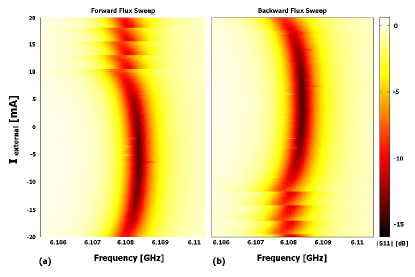
Figure 1: Measured $\left|S_{11}\right|$ at input power $P_{\mathrm{in}}=-95$dBm for forward (a) and backward (b) magnetic flux sweep. In this sample $\beta_{L}=20,$ and the response is highly hysteretic.

As is mentioned in the Suchoi et al. (2009), as the input power is increased the response becomes non-hysteretic. The gradual transition between the hysteretic region to the non-hysteretic one is seen in Fig. 2 below, which shows the difference in the measured resonance frequency of the first mode obtained from increased flux sweep $\left(f_{\mathrm{1inc}}\right)$ and decreased flux sweep $\left(f_{\mathrm{1dec}}\right)$ at different input powers. Dark blue in the color map corresponds to no difference, namely to monostable regions, whereas in the red regions, where a large difference is observed, the system is bistable. As can be clearly seen from the figure, the bistable regions shrink as the input power is increased. The experimental results suggest that the critical current of the nanobridges drops as the input power is increased, and consequently the response becomes non-hysteretic due to the resultant smaller value of the screening parameter $\beta_{L}$. We hypothesize that the drop in the critical current occurs due to heating of the nanobridges by the input power.

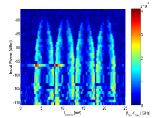
Figure 2: The difference between the measured resonance frequencies obtained in the increasing flux sweep ($f_{\mathrm{1inc}})$ and the decreasing flux sweep ($f_{\mathrm{1dec}})$ of the first (detector) mode. The dark blue areas correspond to monostable regions, namely, the same resonance frequency is measured for both the increased and decreased sweep. The red indicates the regions where the system is bistable.

To estimate the effect of heating, we assume the case where the substrate is isothermal and that the heat is mainly dissipated down into the substrate rather than along the film Johnson et al. (1996). Moreover, we assume that most of the externally injected power into the resonator is dissipated near the nanobridges, where, the current density obtains its largest value. By estimating the heat transfer coefficient per unit area between each nanobridge and the substrate beneath it ($100\operatorname{nm}$ SiN on top of high-resistivity Si) to be $\kappa\simeq 1\operatorname{W}\operatorname{cm}^{-2}\operatorname{K}^{-1}$ Monticone et al. (1999); Weiser et al. (1981) and the area of the nanobridge to be $A\simeq\left(50\operatorname{nm}\right)^{2}$one finds that the expected temperature rise for $P_{\mathrm{in}}=-70$ dBm is $\Delta T=P_{\mathrm{in}}/A\kappa\simeq 4\operatorname{K}$.

Since heating is produced by AC current flowing through the nanobridges, it is important to estimate also the thermal rate, which characterizes the inverse of the typical time scale of thermalization, and is given by $\gamma_{\mathrm{T}}=A\kappa/C$, where the heat capacity $C$ of the nanobridge is given by $C=C_{v}Ad$, $C_{v}$ is the heat capacity per unit volume, and $d$ is the thickness of the superconducting film. Using the estimate $C_{v}\simeq 10^{-3}\operatorname{J}\operatorname{cm}^{-3}\operatorname{K}^{-1}$ Weiser et al. (1981) one finds $\gamma_{\mathrm{T}}\simeq 0.1\operatorname{GHz}$. Since the frequency of the AC heating current is 1-2 orders of magnitude higher, we conclude that to a good approximation the temperature of the nanobridges can be considered as stationary in the steady state.

References

- Suchoi et al. (2009) O. Suchoi, B. Abdo, E. Segev, O. Shtempluck, M. P. Blencowe, and E. Buks, arXiv:0901.3133v1 (2009).
- Hao et al. (2008) L. Hao, J. C. Macfarlane, J. C. Gallop, D. Cox, J. Beyer, D. Drung, and T. Schurig, Applied Physics Letters 92, 192507 (pages 3) (2008), URL http://link.aip.org/link/?APL/92/192507/1.
- Hao et al. (2007) L. Hao, J. C. Macfarlane, J. C. Gallop, D. Cox, P. Joseph-Franks, D. Hutson, J. Chen, and S. K. H. Lam, IEEE Transactions on Instrumentation and Measurement 56, 392 (2007).
- Bell et al. (2003) C. Bell, G. Burnell, D.-J. Kang, R. H. Hadfield, M. J. Kappers, and M. G. Blamire, Nanotechnology 14, 630 (2003), URL http://stacks.iop.org/0957-4484/14/630.
- Datesman et al. (2005a) A. Datesman, J. Schultz, A. Lichtenberger, D. Golish, C. Walker, and J. Kooi, IEEE Transactions on Applied Superconductivity 15, 928 (2005a).
- Troeman et al. (2007) A. Troeman, H. Derking, B. Borger, J. Pleikies, D. Veldhuis, and H. Hilgenkamp, Nano Letters 7, 2152 (2007), ISSN 1530-6984, URL http://pubs3.acs.org/acs/journals/doilookup?in_doi=10.1021/nl%070870f.
- Datesman et al. (2005b) A. Datesman, J. Schultz, T. Cecil, C. Lyons, and A. Lichtenberger, IEEE Transactions on Applied Superconductivity 15, 3524 (2005b), ISSN 1051-8223.
- Clark et al. (2001) T. D. Clark, R. J. Prance, R. Whiteman, H. Prance, M. J. Everitt, A. R. Bulsara, and J. F. Ralph, Journal of Applied Physics 90, 3042 (2001), URL http://link.aip.org/link/?JAP/90/3042/1.
- Blencowe and Buks (2007) M. P. Blencowe and E. Buks, Phys. Rev. B 76, 14511 (2007).
- Nation et al. (2008) P. D. Nation, M. P. Blencowe, and E. Buks, Phys. Rev. B 78, 104516 (2008).
- Granata et al. (2008) C. Granata, E. Esposito, A. Vettoliere, L. Petti, and M. Russo, Nanotechnology 19, 275501 (2008).
- Hasselbach et al. (2002) K. Hasselbach, D. Mailly, and J. Kirtley, Journal of Applied Physics 91, 4432 (2002).
- Hasselbach et al. (2000) K. Hasselbach, C. Veauvy, and D. Mailly, Physica C Superconductivity 332, 140 (2000).
- Baratoff et al. (1970) A. Baratoff, J. A. Blackburn, and B. B. Schwartz, Phys. Rev. Lett. 25, 1096 (1970).
- Likharev (1979) K. K. Likharev, Rev. Mod. Phys. 51, 101 (1979).
- Likharev and Yakobson (1975) K. K. Likharev and L. A. Yakobson, Sov. Phys. - Tech. Phys. (Engl. Transl.) 20, 950 (1975).
- Gumann et al. (2007) A. Gumann, T. Dahm, and N. Schopohl, Physical Review B (Condensed Matter and Materials Physics) 76, 064529 (pages 14) (2007), URL http://link.aps.org/abstract/PRB/v76/e064529.
- Podd et al. (2007) G. J. Podd, G. D. Hutchinson, D. A. Williams, and D. G. Hasko, Physical Review B (Condensed Matter and Materials Physics) 75, 134501 (2007).
- Pronin et al. (1998) A. V. Pronin, M. Dressel, A. Pimenov, A. Loidl, I. V. Roshchin, and L. H. Greene, Phys. Rev. B 57, 14416 (1998).
- Maxfield and McLean (1965) B. W. Maxfield and W. L. McLean, Phys. Rev. 139, A1515 (1965).
- Golubov et al. (2004) A. A. Golubov, M. Y. Kupriyanov, and E. Il’ichev, Rev. Mod. Phys. 76, 411 (2004).
- Troeman et al. (2008) A. G. P. Troeman, S. H. W. van der Ploeg, E. Il’Ichev, H.-G. Meyer, A. A. Golubov, M. Y. Kupriyanov, and H. Hilgenkamp, Physical Review B (Condensed Matter and Materials Physics) 77, 024509 (pages 5) (2008), URL http://link.aps.org/abstract/PRB/v77/e024509.
- Mitra et al. (2008) K. Mitra, F. W. Strauch, C. J. Lobb, J. R. Anderson, F. C. Wellstood, and E. Tiesinga, Physical Review B (Condensed Matter and Materials Physics) 77, 214512 (pages 10) (2008), URL http://link.aps.org/abstract/PRB/v77/e214512.
- Ralph et al. (1996) J. F. Ralph, T. D. Clark, R. J. Prance, H. Prance, and J. Diggins, J. Phys.: Condens. Matter 8, 10753 (1996).
- Buks et al. (2008) E. Buks, E. Arbel-Segev, S. Zaitsev, B. Abdo, and M. P. Blencowe, Europhys. Lett. 81, 10001 (2008).
- Buks et al. (2007) E. Buks, S. Zaitsev, E. Segev, B. Abdo, and M. P. Blencowe, Phys. Rev. E 76, 26217 (2007).
- Littlejohn and Flynn (1991) R. G. Littlejohn and W. G. Flynn, Phys. Rev. A 44, 5239 (1991).
- Panati et al. (2002) G. Panati, H. Spohn, and S. Teufel, Phys. Rev. Lett. 88, 250405 (2002).
- Yurke and Buks (2006) B. Yurke and E. Buks, J. Lightwave Tech. 24, 5054 (2006).
- Tesche and Clarke (1977) C. D. Tesche and J. Clarke, J. low Temp. Phys. 29, 301 (1977).
- Johnson et al. (1996) M. W. Johnson, A. M. Herr, and A. M. Kadin, J. Appl. Phys. 79, 7069 (1996).
- Monticone et al. (1999) E. Monticone, V. Lacquaniti, R. Steni, M. Rajteri, M. Rastello, and L. Parlato, IEEE Trans. Appl. Super. 9, 3866 (1999).
- Weiser et al. (1981) K. Weiser, U. Strom, S. A. Wolf, and D. U. Gubser, J. Appl. Phys. 52, 4888 (1981).