Phase diagram of the frustrated, spatially anisotropic $S=1$ antiferromagnet on a square lattice

Abstract

We study the $S=1$ square lattice Heisenberg antiferromagnet with spatially anisotropic nearest neighbor couplings $J_{1x}$, $J_{1y}$ frustrated by a next-nearest neighbor coupling $J_{2}$ numerically using the density-matrix renormalization group (DMRG) method and analytically employing the Schwinger-Boson mean-field theory (SBMFT). Up to relatively strong values of the anisotropy, within both methods we find quantum fluctuations to stabilize the Néel ordered state above the classically stable region. Whereas SBMFT suggests a fluctuation-induced first order transition between the Néel state and a stripe antiferromagnet for $1/3\leq J_{1x}/J_{1y}\leq 1$ and an intermediate paramagnetic region opening only for very strong anisotropy, the DMRG results clearly demonstrate that the two magnetically ordered phases are separated by a quantum disordered region for all values of the anisotropy with the remarkable implication that the quantum paramagnetic phase of the spatially isotropic $J_{1}$-$J_{2}$ model is continuously connected to the limit of decoupled Haldane spin chains. Our findings indicate that for $S=1$ quantum fluctuations in strongly frustrated antiferromagnets are crucial and not correctly treated on the semiclassical level.

I Introduction

A striking commonality between the recently discovered iron pnictides superconductorsKamihara et al. (2008); Takahashi et al. (2008); Ren et al. (2008); Chen et al. (2008a, b) and the high-$T_{c}$ cuprates is that in both cases superconductivity emerges on doping antiferromagnetic parent compounds. In trying to unravel the mechanisms of superconductivity frustrated quantum antiferromagnets on the square lattice have been subject to intense research over the last decades with particular interest in the extreme quantum limit $S=\frac{1}{2}$ relevant for the cuprates, whereas the interest in higher spin values increased tremendously with the discovery of the pnictides.

Thereby, the Heisenberg model with antiferromagnetic exchange couplings $J_{1}$ and $J_{2}$ between nearest neighbor (NN) and next-nearest neighbor (NNN) has served as a prototype model for studying magnetic frustration. On a classical level, one finds Néel order to be stable for $J_{2}/J_{1}\leq 1/2$ whereas for larger ratios the classical ground state is give by a stripe-antiferromagnet with ordering wave-vector $(\pi,0)$. Not surprisingly, the $J_{1}$-$J_{2}$ model has been used to rationalize the $(\pi,0)$ magnetismde la Cruz et al. (2008) of the iron pnictide superconductors and to subsequently calculate the magnetic excitation spectraYao and Carlson (2008); Zhao et al. (2008a) where the incorporation of a strong anisotropy between the NN couplings turned out to be necessary to reproduce the low energy spin-wave excitations. Recently, it has been suggested that the strong anisotropies in the magnetismZhao et al. (2008a), but also in electronic propertiesMcGuire et al. (2008) of the pnictides originate in the coupling to orbital degrees of freedom arising from an orbital degeneracy of an intermediate $S=1$ spin stateKrüger et al. (2008). Even if the charge degrees of freedom are not completely localized, the $J_{1}$-$J_{2}$ model can be used as the starting point for a symmetry-based analysis of magnetism and superconductivity in the iron-based superconductors Xu et al. (2008); Fang et al. (2008).

The $1/S$ expansion serves as a natural starting point to investigate the stability of the classical orders against quantum fluctuations which are expected to induce a paramagnetic phase near $J_{2}/J_{1}=1/2$ where both orders compete. Indeed, on the level of lowest order linear spin-wave theory one finds an intermediate paramagnetic phase for all spin valuesChandra and Doucot (1988). However, the incorporation of spin-wave interactions within a modified spin-wave theory (MSWT)Xu and Ting (1990); Gochev (1995) or the SBMFTMila et al. (1991) drastically changes this picture. Within both approaches one finds a dramatic stabilization of the classical orders by quantum fluctuation for the Néel order even up to values considerably larger than the classical threshold value $J_{2}/J_{1}=1/2$. This has been interpreted as an order-out-of-disorder phenomenon giving rise to a fluctuation induced first order transition between the two orders. This picture has been confirmed recently by a functional one-loop renormalization group analysisKrüger and Scheidl (2006) where it was shown that the Néel phase becomes unstable towards a fluctuation induced first order transition for $S>0.68$.

Surely, it is questionable if the semiclassical treatment can correctly account for the quantum fluctuations in the regime of strong frustration and small spins. In fact, in the case $S=\frac{1}{2}$ various numerical studies including exact diagonalizationDagotto and Moreo (1989); Schulz and Ziman (1992); Schulz et al. (1996); Sindzingre (2004), variational Monte CarloCapriotti and Sorella (2000); Capriotti et al. (2001) series expansionGelfand et al. (1989); Gelfand (1990); Singh et al. (1999); Sushkov et al. (2001, 2002) as well as the coupled cluster approachBishop et al. (1998) give the consistent picture that in the regime $0.4\lesssim J_{2}/J_{1}\lesssim 0.6$ no magnetic order is present clearly indicating that the aforementioned semiclassical treatments overestimate the stability of the ordered states. Another key observation of the series expansion and in particular of the unbiased exact diagonalization studies is that in the paramagnetic phase the lattice symmetry is spontaneously broken due to the formation of columnar valence bond solid order. Such states have been predicted beforeRead and Sachdev (1989, 1990) on the basis of a large $N$ treatment for non frustrated systems in the absence of long-range antiferromagnetic order. These depend however crucially on the value of the spin, revealing the subtle workings of the spin Berry phases (see e.g. [Sachdev, 2008] and references therein). For $S=\frac{1}{2}$ these act to give a special stability to ’valence bond’ pair singlets involving nearest-neighbor spins, and the quantum disordered phases are actually valence bond crystals breaking the translational symmetry of the square lattice further to fourfold degenerate spin-Peierls states. But for $S=1$ the Berry phases act in favor of the formation of ’chain singlets’Read and Sachdev (1989, 1990) that can stack either along the $x$ or $y$ direction of the square lattice yielding a twofold degenerate ground state.

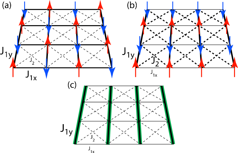
Figure 1: The model studied in this paper consists of a $S=1$ Heisenberg system with spatially anisotropic nearest-neighbor couplings $J_{1x}$, $J_{1y}$ and isotropic next-nearest-neighbor couplings $J_{2}$. Pending the balance of these couplings one finds either a simple staggered- (a) or ’stripe’ (b) antiferromagnetic order. In the limit of isolated chains a stack of isolated Haldane spin chains is formed (c) and based on our DMRG calculations we could conclude that these survive all the way to the isotropic limit in the vicinity of the point of maximal frustration ($J_{2}/J_{1}=0.5$).

In this paper we investigate the $S=1$ version of the spatially anisotropic $J_{1}$-$J_{2}$ model, given by the Hamiltonian

$$H=J_{1x}\sum_{\langle i,j\rangle_{x}}\mathbf{S}_{i}\mathbf{S}_{j}+J_{1y}\sum_{\langle i,j\rangle_{y}}\mathbf{S}_{i}\mathbf{S}_{j}+J_{2}\sum_{\langle\langle i,j\rangle\rangle}\mathbf{S}_{i}\mathbf{S}_{j},$$ (1)

where the first two sums run over NN spins with exchange couplings $J_{1x}\leq J_{1y}$ in $x$ and $y$ directions, respectively, and the third sum runs over all NNN pairs with exchange couplings $J_{2}$ as illustrated in Fig 1. We note that both the spatially isotropic $J_{1}$-$J_{2}$ model as well as the decoupled Haldane spin-chain limit appear as special cases of Hamiltonian (1).

Unlike for $S=\frac{1}{2}$ this model has been hardly explored for $S=1$ despite the potential relevance for the iron pnictides, and to best of our knowledge exact diagonalization studies are not available. In a very recent coupled cluster treatmentBishop et al. (2008) it has been found that at the isotropic point $J_{1x}=J_{1y}=J_{1}$ the Néel and stripe ordered phases are separated by a first order transition at $J_{2}/J_{1}\approx 0.55$ slightly smaller than the MSWTXu and Ting (1990); Gochev (1995) and SBMFTMila et al. (1991) results and that the transition remains first order up to an anisotropy $J_{1x}/J_{1y}\approx 0.66$. For stronger anisotropies the authors find continuous transitions very close to the classical transition line $J_{2}=J_{1x}/2$, although they were not able to resolve an intermediate paramagnetic region within the numerical resolution. On contrary, a two step DMRG studyMoukouri (2006) at the particular point $J_{1x}/J_{1y}=0.2$ indicated a much wider non-magnetic region with a spin-gap reaching its maximum $\Delta\approx 0.39J_{1y}$ close to the maximally frustrated point $J_{2}/J_{1y}=0.1$, which is only slightly below the gap $\Delta_{H}\approx 0.41J$ [Sorensen and Affleck, 1993] of an isolated Haldane chainHaldane (1983a, b).

Starting from the Haldane chain limit ($J_{1x}=J_{2}=0$) it has been predicted by Monte Carlo simulationsTodo et al. (2001) as well as analyticallyAnfuso and Rosch (2007) that an infinitesimal coupling $J_{1x}$ leads to the destruction of the topological string orderdenNijs and Rommelse (1989) of the Haldane chain. However, due to the protection by the finite energy gap of the spin-1 Haldane chain all other ground-state properties as well as the thermodynamics are only minimally affected by a small interchain coupling $J_{1x}$ and a finite, albeit smallKim and Birgeneau (2000); Matsumoto et al. (2001); Alet and Sorensen (2002); Zinke et al. (2008) coupling is necessary to establish magnetic long range order. Whereas a similar reasoning should hold for a vanishing NN coupling perpendicular to the chains ($J_{1x}=0$) and small diagonal coupling $J_{2}$ the Haldane chain phase seems to be considerably more stable against the simultaneous increase of the two mutually frustrating couplings $J_{1x}$ and $J_{2}$ as indicated by two step DMRG results showing an almost negligible reduction of the spin gap for moderate interchain couplingsMoukouri (2006). This suggests that the paramagnetic phase of the frustrated two dimensional spin model can be viewed as a continuation of the Haldane spin chain. Recently, based on a theoretical method with a continuous deformation of the $J_{1}$-$J_{2}$ model, the ground state at the special isotropic case $J_{2}=J_{1}/2$ has been conjecturedCai et al. (2007) to be a two-fold degenerate valence bond solid state along either the horizontal or vertical direction of the square lattice. The main result of this paper is that by employing DMRG and by studying systematically how matters evolve as function of increasing anisotropy we arrive at solid evidence for the smooth continuation between the Haldane chain phase and an isotropic disordered phase near $J_{2}=J_{1}/2$.

Since for $S=1$ exact diagonalization is restricted to very small system sizes and since the quantum Monte Carlo method suffers from the infamous sign problem in the presence of frustration we employ the DMRG methodR.White (1992) to map out the phase diagram of the spatially anisotropic $J_{1x}-J_{1y}-J_{2}$ model (1) over the whole parameter range including the decoupled Haldane spin chains and the isotropic $J_{1}$-$J_{2}$ model as limiting cases. The DMRG has the merits of not being biased as analytical treatments based on $1/S$ or $1/N$ expansions, being capable of dealing with frustrated systems, and allowing to investigate much bigger system than possible with exact diagonalization. Moreover, it is capable of reproducing the spin gap of the decoupled Haldane chain limit with high accuracyMoukouri (2006). The resulting phase diagram is contrasted by analytical results we obtain within a generalization of the SBMFT to the anisotropic system.

The remainder of the paper is organized as follows. In Sec. II we outline the SBMFT and calculate the resulting phase diagram which is used for comparison with the numerical results. In Sec. III we use the DMRG to construct the phase diagram by a careful finite-size analysis of the magnetic structure factor at the ordering wave vectors of the two magnetically ordered phases as well as of the spin-gap in the non magnetic region as a function of the NNN coupling $J_{2}$ for various ratios of the NN couplings $J_{1x}$ and $J_{1y}$. Finally, in Sec. IV the results obtained within the two methods are compared and the shortcomings of the semiclassical approach are highlighted. Further, the potential relevance of our findings for the iron pnictides is discussed.

II SBMFT

In this section we generalize the SBMF calculation for the isotropic $J_{1}$-$J_{2}$-modelMila et al. (1991) to the case of anisotropic nearest-neigbor exchange couplings. For abbreviation we define $J_{x}:=J_{1x}$, $J_{y}:=J_{1y}$, and $J_{d}:=J_{2}$. Assuming $J_{x}\leq J_{y}$, the classical ground states are given by a Néel ordered state with an ordering wavevector ${\bm{Q}}=(\pi,\pi)$ for $J_{d}/J_{x}\leq 1/2$ and by a columnar antiferromagnetic state with ${\bm{Q}}=(0,\pi)$ for $J_{d}/J_{x}>1/2$. Following the previous calculations, we perform a spin rotation ${\tilde{S}}^{x}_{i}=\sigma_{i}S^{x}_{i}$, ${\tilde{S}}^{y}_{i}=\sigma_{i}S^{y}_{i}$, ${\tilde{S}}^{z}_{i}=S^{z}_{i}$, where $\sigma_{i}=\exp(i{\bm{Q}}{\bm{r}}_{i})=\pm 1$ with ${\bm{Q}}$ the ordering wavevectors of the two classical orders, and represent the rotated spin operators in terms of Schwinger bosons $b_{i,\uparrow}$, $b_{i,\downarrow}$ as

$${\tilde{\bm{S}}}_{i}=\frac{1}{2}b_{i,\nu}^{\dagger}{\bm{\sigma}}_{\nu,\nu^{\prime}}b_{i,\nu^{\prime}}.$$ (2)

Here ${\bm{\sigma}}=(\sigma^{x},\sigma^{y},\sigma^{z})$ with $\sigma^{\alpha}$ the standard Pauli matrices. The constraint $b_{i,\nu}^{\dagger}b_{i,\nu}=2S$ ensures that $\langle{\bm{S}}^{2}\rangle=S(S+1)$. The Hamiltonian (1) can then be rewritten in the compact form

$${\mathcal{H}} = \frac{1}{2}\sum_{(i,j)}J_{ij}\left[\frac{\sigma_{i}\sigma_{j}+1}{2}(F_{ij}^{\dagger}F_{ij}-2S^{2})\right.$$ (3)

$$\left.+\frac{\sigma_{i}\sigma_{j}-1}{2}(G_{ij}^{\dagger}G_{ij}-2S^{2})\right],$$

where the sum runs over all bonds and we have introduced the bond operators $F_{ij}^{\dagger}=b_{i,\nu}^{\dagger}b_{j,\nu}$ and $G_{ij}^{\dagger}=b_{i,\nu}^{\dagger}b_{j,-\nu}^{\dagger}$. A mean-field decoupling is then performed with respect to the order parameters $f_{ij}=\langle F_{ij}^{\dagger}\rangle/2$ and $g_{ij}=\langle G_{ij}^{\dagger}\rangle/2$. For the Néel ordered phase we have to introduce fields $g_{x}$, $g_{y}$ for the non-frustrated nearest-neigbor bonds and $f_{d}$ for frustrated NNN bonds whereas the $(0,\pi)$-phase is characterized by order-parameter fields $g_{y}$ and $g_{d}$ for the non-frustrated bonds along the y and diagonal directions and $f_{x}$ for the frustrated x-bonds. The local constraints are replaced by a global one and treated with a Lagrange multiplier $\lambda$. The resulting mean-field Hamiltonian, which in momentum space is given by

$${\mathcal{H}}_{\text{mf}} = \int_{\bm{q}}\left[(h_{\bm{q}}+\lambda)(b^{\dagger}_{{\bm{q}}\uparrow}b_{{\bm{q}}\uparrow}+b^{\dagger}_{-{\bm{q}}\downarrow}b_{-{\bm{q}}\downarrow})\right.$$ (4)

$$\left.-\Delta_{\bm{q}}(b^{\dagger}_{{\bm{q}}\uparrow}b^{\dagger}_{-{\bm{q}}\downarrow}+b_{{\bm{q}}\uparrow}b_{-{\bm{q}}\downarrow})\right],$$

is easily diagonalized by a Bogolioubov transformation yielding the dispersion

$$\omega_{\bm{q}}=[(h_{\bm{q}}+\lambda)^{2}-\Delta_{\bm{q}}^{2}]^{1/2}$$ (5)

with

$$h_{\bm{q}} = 4f_{d}J_{d}\cos q_{x}\cos q_{y},$$ (6a)

$$\Delta_{\bm{q}} = 2(g_{x}J_{x}\cos q_{x}+g_{y}J_{y}\cos q_{y})$$ (6b)

in the Néel phase and likewise in the $(0,\pi)$ phase

$$h_{\bm{q}} = 2f_{x}J_{x}\cos q_{x},$$ (7a)

$$\Delta_{\bm{q}} = 2g_{y}J_{y}\cos q_{y}+4g_{d}J_{d}\cos q_{x}\cos q_{y}.$$ (7b)

The Lagrange multiplier in the ordered phases is determined by the requirement that $\omega_{\bm{Q}}=0$ for the corresponding ordering wavevectors yielding $\lambda=2(g_{x}J_{x}+g_{y}J_{y})-4f_{d}J_{d}$ in the Néel and $\lambda=2(g_{y}J_{y}-f_{x}J_{x})+4g_{d}J_{d}$ in the $(0,\pi)$-phase. The reduced moment $S^{*}$ in the ordered phases is determined by

$$S^{*}=S-\frac{1}{2}\left(\int_{\bm{q}}\frac{h_{q}+\lambda}{\omega_{q}}-1\right).$$ (8)

Naturally, one might expect that quantum fluctuations tend to destabilize the classical orders introducing an intermediate paramagnetic phase. In this case the second order transitions between the two different magnetic orders are determined by the lines where the corresponding magnetizations go to zero, $S^{*}\to 0$. However, the analysis of the isotropic modelMila et al. (1991) ($J_{x}=J_{y}$) shows that the quantum fluctuations can lead to a significant stabilization of the Néel order leading to a region where $S^{*}_{(\pi,\pi)}>0$ and $S^{*}_{(0,\pi)}>0$. In this region which is expected to persist for not too strong anisotropy, a discontinuous first order transition between the two different magnetic orders is likely and can be estimated from a comparison of the ground-state energies which immediately follow from Eq. (3) as

$$E_{(\pi,\pi)} = -J_{x}(2g_{x}^{2}-S^{2})-J_{y}(2g_{y}^{2}-S^{2})$$ (9a)

$$+2J_{d}(2f_{d}^{2}-S^{2})$$

$$E_{(0,\pi)} = J_{x}(2f_{x}^{2}-S^{2})-J_{y}(2g_{y}^{2}-S^{2})$$ (9b)

$$-2J_{d}(2g_{d}^{2}-S^{2}).$$

The order parameter fields entering the mean-field Hamiltonian (4) have to be determined self consistently. Using the above Bogoliubov transformation we obtain for the Néel ordered phase

$$g_{x} = S^{\ast}+\int_{\bm{q}}\frac{\Delta_{\bm{q}}}{2\omega_{\bm{q}}}\cos q_{x},$$ (10a)

$$g_{y} = S^{\ast}+\int_{\bm{q}}\frac{\Delta_{\bm{q}}}{2\omega_{\bm{q}}}\cos q_{y},$$ (10b)

$$f_{d} = S^{\ast}+\int_{\bm{q}}\frac{h_{\bm{q}}+\lambda}{2\omega_{\bm{q}}}\cos q_{x}\cos q_{y},$$ (10c)

whereas in the $(0,\pi)$ phase the self-consistency equations for the order-parameter fields are given by

$$f_{x} = S^{*}+\int_{\bm{q}}\frac{h_{\bm{q}}+\lambda}{2\omega_{\bm{q}}}\cos q_{x},$$ (11a)

$$g_{y} = S^{*}+\int_{\bm{q}}\frac{\Delta_{\bm{q}}}{2\omega_{\bm{q}}}\cos q_{y},$$ (11b)

$$g_{d} = S^{*}+\int_{\bm{q}}\frac{\Delta_{\bm{q}}}{2\omega_{\bm{q}}}\cos q_{x}\cos q_{y}.$$ (11c)

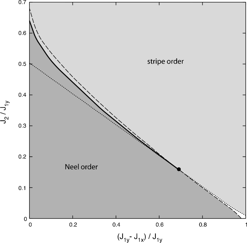
Figure 2: Phase diagram for $S=1$ as a function of and anisotropy $\alpha=(J_{1y}-J_{1x})/J_{1y}>0$ between the nearest neigbor exchange couplings and relative strength of the next nearest neighbor coupling $J_{2}/J_{1y}$ obtained within SBMFT. Up to an anisotropy $\alpha\approx 0.66$ the $(\pi,\pi)$ and $(0,\pi)$ antiferromagnetic orders are separated by a first order transition (solid line). At the tricritical point the first-order line splits into two second-order lines (dashed and dotted) separating the two magnetic phases from a gapped non-magnetic phase.

The resulting phase diagram for $J_{1x}\leq J_{1y}$ is shown in Fig. 2 as a function of the anisotropy $\alpha=(J_{1y}-J_{1x})/J_{1y}$ between the NN exchange couplings and of the relative strength $\beta=J_{2}/J_{1y}$ of the NNN coupling. In agreement with earlier studies of the isotropic limit $J_{1x}=J_{1y}=J_{1}$ within SBMFT and MSWT we find a dramatic stabilization of the Néel order above the classical value and a large region $0.51\lesssim\beta\lesssim 0.68$ where the two competing orders are potentially stable, indicated by $S_{(\pi,\pi)}^{\ast}>0$ and $S_{(0,\pi)}^{\ast}>0$. The crossing of the self-consistently determined energies of the two states suggests a first order transition at $\beta\approx 0.64$ considerably larger than the classical value $1/2$ and about 10 percent bigger than the coupled cluster resultBishop et al. (2008). Although the region of coexistence is considerably narrowed by a small anisotropy we find it to persist up to $\alpha\approx 0.66$ where the first order line terminates. The existence of such a tricritical point was also suggested by the coupled cluster analysis although located at a much smaller anisotropy $\alpha\approx 0.34$. For anisotropies $\alpha>0.66$ we find an intermediate non-magnetic region ($S_{(\pi,\pi)}^{\ast}=S_{(0,\pi)}^{\ast}=0$) separating the two ordered phases. This region is found to be very narrow and close to the classical phase boundary $\beta=(1-\alpha)/2$.

Although the existence of a tricritical point and of a very narrow paramagnetic strip terminating at the Haldane chain limit $J_{1x}=J_{2}=0$ is in qualitative agreement with the coupled cluster resultsBishop et al. (2008) the small width of the paramagnetic region is in disagreement with other available numerical results. For $J_{1x}/J_{1y}=0.2$ ($\alpha=0.8$) a two step DMRG calculationMoukouri (2006) shows a much wider non magnetic region centered around the classical transition point $J_{2}/J_{1y}=0.1$. Interestingly, the spin gap at this maximally frustrated point is almost identical to that of an isolated Haldane chain suggesting that even for relatively strong interchain couplings one dimensional Haldane chain physics is still important. This is certainly missed by the SBMF calculation which treats the spin as a continuous variable and does not distinguish between integer and half-integer spins crucial for the existence of the Haldane spin gap. Moreover, it has been established within quantum Monte Carlo calculationsKim and Birgeneau (2000); Matsumoto et al. (2001); Alet and Sorensen (2002) that for $J_{2}=0$ the transition between the Néel ordered phase and the gapped non-magnetic phase is located at $J_{1x}/J_{1y}=0.044$, again indicating that the paramagnetic region close to the Haldane chain limit is considerably wider than suggested by both the SBMFT and the coupled cluster resultsBishop et al. (2008). Since for $J_{2}=0$ the system is not frustrated quantum Monte Carlo can be considered exact in this regime.

We have also calculated the transition out of the $(0,\pi)$ state in linear spin-wave theory, for comparison to the SBMFT calculation and to preliminary neutron scattering results on the pnictides that found $(0,\pi)$ order but with a small moment. This method computes the reduction of the classical antiferromagnetic moment due to zero-point excitations of spin waves (which captures the $1/S$ correction to the classical moment in a large-$S$ expansion). The transition line out of the ordered phase is estimated as the point where the correction is as large as the original moment.

We assume three antiferromagnetic couplings: $J_{1x}$, $J_{1y}$, and $J_{2}$ with $J_{1y}>J_{1x}$ and that we are in a $(0,\pi)$ ordered phase, which requires (as is evident from the formula below) that $J_{1x}<2J_{2}$. The dispersion relation for spin-wave excitations was previously obtained for this anisotropic $J_{1}$-$J_{2}$ model in Ref. Krüger et al., 2008. The integral for the correction to the classical moment around the $(0,\pi)$ case is, in units of the Bohr magneton and with lattice spacing $a=1$,

$$\Delta m=\int_{[0,2\pi]^{2}}\frac{\textrm{d}^{2}\mathbf{k}}{(2\pi)^{2}}\left(\frac{1}{\sqrt{1-\cos^{2}(k_{y})/f(k_{x})^{2}}}-1\right)\quad$$ (12)

with

$$f(k_{x})=\frac{2J_{2}+J_{1y}-J_{1x}[1-\cos(k_{x})]}{2J_{2}\cos(k_{x})+J_{1y}}.$$ (13)

The transition is found numerically to lie very close to the classical transition line $J_{1x}=2J_{2}$: the normalized difference $(J_{2}^{c}-J_{1x}/2)/J_{1y}$, where $J_{2}^{c}$ is the critical coupling where the correction is equal to the original moment, is always less than 2% for $0<J_{1x}<0.99J_{1y}.$ Significant reduction of the ordered moment also occurs only near the classical transition line. The primary difference from the SBMFT calculation is that the spin-wave calculation always predicts a paramagnetic phase between stripe and Neél order. The width of this paramagnetic phase is much smaller in either approach than in the DMRG calculation of the following section, because these analytical approaches do not capture the strong quantum fluctuations that favor the Haldane phase.

III DMRG

The above SBMFT has clearly shown an interesting narrow boundary region between the Néel and stripe ordered phases in the phase diagram of Fig. 2, where the quantum fluctuations are expected to become very important. Most interestingly, it suggests an increasing tendency towards a fluctuation induced first order transition on approaching the isotropic point $J_{1x}=J_{1y}$. However, the comparison with previous numerical resultsMoukouri (2006); Kim and Birgeneau (2000); Matsumoto et al. (2001); Alet and Sorensen (2002) indicates that the SBMFT tends to overestimate the stability of the magnetically ordered phases, surely close to the Haldane chain limit but presumably also for larger values of $J_{1x}$ and $J_{2}$. In the following we shall refine the boundary region by using DMRG method.

In the following DMRG calculation, we will set $J_{1y}=J_{1}$ as energy unit, and a periodic boundary condition (PBC) is used and in each DMRG block up to $m=3200$ states are to be kept with the truncation error in the order of or less than $10^{-5}$.

III.1 Isotropic case with $J_{1x}=J_{1y}=J_{1}$

Let us first consider the isotropic case $J_{1x}=J_{1y}=J_{1}$ where the SBMFT suggests the strongest tendency towards a first order transition although the transition point $J_{2}/J_{1}\approx 0.64$ obtained from a comparison of the energy minima seems to be suspiciously high compared to the classical transition point $J_{2}/J_{1}=0.5$. Fig. 3 shows the ground state energy per site calculated by DMRG with the sample size varying from $N=4\times 4$ ($16$ sites) up to $N=8\times 8$ ($64$ sites). The ground state energy reaches the maximum with $J_{2}$ between $0.54J_{1}$ and $0.58J_{1}$, which becomes sharper with the increase of sample size, indicating a region with possible phase transitions below the first order transition point obtained in SBMFT but still notable above the classical transition.

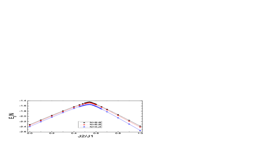
Figure 3: (color online) The ground-state energy per site at different system size $N=4\times 4$ (blue triangle), $6\times 6$ (red circle) and $8\times 8$ (black square), for the isotropic case with $J_{1x}=J_{1y}=J_{1}$.

We examine such a region by calculating the magnetic structure factor $S_{z}(\mathbf{q})$, defined by

$$S_{z}(\mathbf{q})={\frac{1}{N}}{\sum_{i,j}}e^{-i\mathbf{q}(\mathbf{r}_{i}-\mathbf{r}_{j})}\langle S_{i}^{z}S_{j}^{z}\rangle.$$

As expected, we find that $S_{z}(\mathbf{q})$ shows a dramatic change from peaking at ${\bm{Q}}=(\pi,\pi)$ (the Néel order) to ${\bm{Q}}=(0,\pi)$ (the stripe order) with increasing $J_{2}/J_{1}$. Fig. 4 (a) and (b) illustrate $S_{z}(\mathbf{q})/N$ vs. $J_{2}/J_{1}$ for system sizes $N=4\times 4$, $6\times 6$ and $8\times 8$, as well as the thermodynamic limit values obtained by a finite size scaling. Here we have used the quadratic function $f(x)=A+Bx+Cx^{2}$ with $x=\frac{1}{N}$ to perform the finite-size scaling.

The Néel order transition point is found at $J_{2}/J_{1}\approx 0.525$ in Fig. 4(a), which is clearly distinct from the stripe order tranistion point at $J_{2}/J_{1}\approx 0.55$ in Fig. 4(b) indicating that the two magnetically ordered phases are separated by an intermediate non-magnetic region.

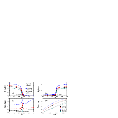
Figure 4: (color online) The evolution of the peak values of the structure factors, $S_{z}(\pi,\pi)/N$ (a), $S_{z}(0,\pi)/N$ (b), and of the spin-1 gap (c), at three different size $N=4\times 4$, $6\times 6$ and $8\times 8$, as well as their thermodynamic limit extrapolations in the isotropic case $J_{1x}=J_{1y}=J_{1}=1$. The finite-size scaling for the spin-1 gap is shown in (d).

To independently verify the above results, we also calculate the spin-1 gap $\Delta E(S=1)\equiv E_{1}(S=1)-E_{0}$ presented in Fig. 4(c) and (d). Fig. 4(d) illustrates the finite-size scaling for the spin gap $\Delta E(S=1)$ at different values of $J_{2}$ using a scaling function $f(x)$. In Fig. 4(c), the evolution of the spin-1 gap as a function of $J_{2}$ is given. In the thermodynamic limit, the transition points determined by the spin-1 gap are at $J_{2}\approx 0.525$ and $J_{2}\approx 0.555$, respectively, which are very close to the previous results determined by the structure factor. Therefore, for the present $S=1$ $J_{1}$-$J_{2}$ model in the isotropic limit, our numerical approach has established an intermediate spin disordered region with a finite spin gap which separates the two ordered magnetic phases.

III.2 Anisotropic case with $J_{1x}<J_{1y}=J_{1}$

Now we consider how the spin disordered phase evolves with the increase of anisotropy at $J_{1x}<J_{1y}=J_{1}$. First we consider the case at $J_{1x}=0.5J_{1}$, and the results are presented in Fig. 5. By using the same finite size scaling procedure, we find that the spin disordered phase is bound by a lower transition point $J_{2}/J_{1}\approx 0.24$ and an upper transition point $J_{2}/J_{1}\approx 0.28$ based on the structure factor calculation. Again the spin gap calculation gives rise to a consistent spin disordered regime between $J_{2}/J_{1}\approx 0.23$ and $J_{2}/J_{1}\approx 0.285$ as shown in Fig. 5 (c).

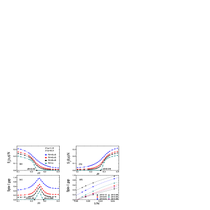
Figure 5: (color online) The peak values, (a) $S_{z}(\pi,\pi)/N,$ (b) $S_{z}(0,\pi)/N$, and (c) the spin-1 gap, versus $J_{2}/J_{1y}$ at $J_{1x}/J_{1y}=0.5$ for different sizes. The finite-size scaling for the spin-1 gap is shown in (d).

In the same regime, with a fixed $J_{2}/J_{1}=0.25$, we have further studied the phase boundaries by varying $J_{1x}/J_{1}$. As shown in Fig. 6, the lower transition point is obtained at $J_{1x}/J_{1}=0.45$ and the upper transition point at $J_{1x}/J_{1}\approx 0.52$, while the finite size scaling for the spin-1 gap results in a similar region between $J_{1x}/J_{1}=0.44-0.54$.

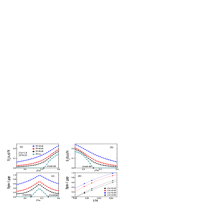
Figure 6: (color online) (a) $S_{z}(\pi,\pi)/N$, (b) $S_{z}(0,\pi)/N$, and (c) the spin-1 gap, versus $J_{1x}/J_{1y}$ at $J_{2}/J_{1y}=0.25$ for different sample sizes. In (d), the finite-size scaling for the spin-1 gap is given.

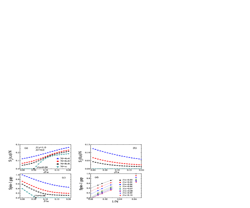
Figure 7: (color online) (a) $S_{z}(\pi,\pi)/N$, (b) $S_{z}(0,\pi)/N$, and (c) the spin-1 gap, versus $J_{1x}/J_{1y}$ at $J_{2}=0$ at different sizes. In (d), the finite-size scaling for the spin-1 gap is given.

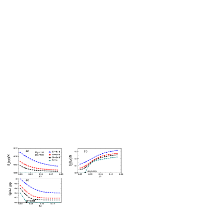
Figure 8: (color online) At $J_{1x}=0$, the structure factors $S_{z}(\pi,\pi)/N$ (a) and $S_{z}(0,\pi)/N$ (b) as well as the spin-1 gap (c) versus $J_{2}/J_{1y}$ are shown at different sizes, including their thermodynamic extrapolations.

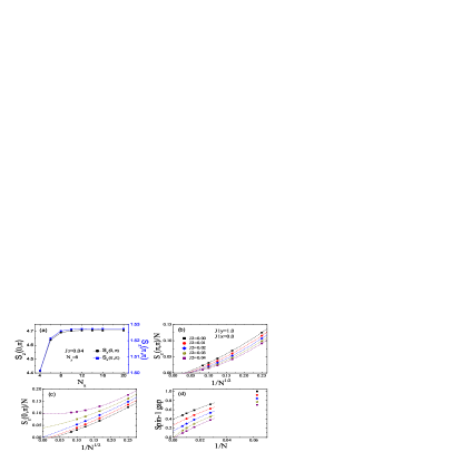
Figure 9: (color online) (a) The size dependence of the structure factor [for a given $N_{y}=$ $6$ (6-leg systems)] at $J_{1x}=0$ and small $J_{2}/J_{1y}$ which quickly saturates at $N_{x}>N_{y}$, indicating that $x=1/N_{y}$ in the scaling function $f(x)$ for the structure factor is more appropriate in this extreme limit. The corresponding finite-size scaling of the structure factors for square samples are illustrated in (b) and (c), respectively. For comparsion, the spin-1 gap at different $J_{2}$ is still well scaled by $x=1/N$ in the scaing function as shown in (d).

In the extreme case at $J_{1x}=0$ and $J_{2}=0$ with $J_{1y}=J_{1}$, the system simply reduces to an array of decoupled $S=1$ spin chains with a finite Haldane gap. Fig. 7 shows how the ground state continuously evolves from that of the well-known decoupled spin chains to the anisotropic 2D case by turning on $J_{1x}/J_{1}$, which remains disordered until the Néel order sets in at $J_{1x}/J_{1}\approx 0.05$ with $S_{z}(\pi,\pi)/N$ becoming finite in the thermodynamic limit. Indeed the corresponding spin-1 gap continuously decreases with the turning on of a finite $J_{1x}$, but only vanishes around $J_{1x}/J_{1}\approx 0.06$ as shown in Fig. 7 (c) and (d).

Now we turn on $J_{2}$. At $J_{1x}=0,$ we find that while the calculated structure factor at $(\pi,\pi)$ continuously reduces as the sample size increases from $N=4\times 4$, $6\times 6$, to $8\times 8$, and is extrapolated to zero by finite size scaling, a finite stripe order $S_{z}(0,\pi)/N$ will emerge at $J_{2}/J_{1y}=0.025$ in the thermodynamic limit, which is further supported by vanishing spin-1 excitation gap at the same point as shown in Fig. 8. It is noted that the best finite scaling for the structure factor here is obtained with using a $f(x)$ with $x=1/\sqrt{N}=1/N_{y},$ for a square lattice $N_{x}=N_{y},$ instead of $x=1/N$ used previously. The justification of such a finite-size scaling for the spin structure factors at $J_{1x}=0$ and small $J_{2}/J_{1y}$ is given in Fig. 9 and its caption.

III.3 Phase diagram

The resulting phase diagram obtained by the DMRG calculations with careful finite size scalings of the magnetic structure factor as well as the spin gap is shown in Fig. 10 as a function of the anisotropy $\alpha=(J_{1y}-J_{1x})/J_{1y}$ between the NN couplings and the relative strength $\beta=J_{2}/J_{1y}$ of the NNN superexchange.

In contrast to the SBMFT which in the regime of small anisotropy $\alpha$ suggests a first order transition between the Néel and stripe ordered phases (see Fig. 2), the DMRG results clearly indicate a paramagnetic strip separating the two magnetically ordered phases for all values of the anisotropy $\alpha$ including the isotropic point $J_{1x}=J_{1y}$ ($\alpha=0$). With increasing $\alpha$ the width of this region is found to slightly increase. Close to the Haldane chain limit the SBMFT predicts an intermediate non magnetic phase, though the width of this region is found to be much larger in the DMRG calculation in quantitative agreement with a previous two step DMRG analysis at fixed $\alpha=0.8$ (Ref. Moukouri, 2006).

For $J_{2}=0$ we can compare our results to recent QMC simulationsKim and Birgeneau (2000); Matsumoto et al. (2001); Alet and Sorensen (2002), which in this regime can be considered exact since the system is not frustrated and QMC is therefore free of any sign problem. Within DMRG we find the transition between the gapped Haldane phase and the Néel ordered phase to occur at $J_{1x}/J_{1y}\approx 0.05$ (see Fig. 10) in good agreement with QMC transition point $J_{1x}/J_{1y}=0.044$. Moreover, in the Haldane chain limit $J_{1x}=J_{2}=0$ we obtain a spin gap $\Delta\approx 0.4$ (see Fig. 7(d)) very close to the exact value $\Delta_{H}=0.41$ for the Haldane spin chainSorensen and Affleck (1993), again demonstrating that the finite size scaling is well converged.

Very interestingly, starting from the Haldane chain limit we find the maximum spin gap in the paramagnetic phase to decrease only very slowly with increasing couplings $J_{1x}$ and $J_{2}$. Up to $J_{1x}/J_{1y}=0.5,$ the gap is almost identical to the Haldane spin gap (see Fig. 5(d)) indicating that the Haldane spin chain is very robust against the simultaneous increase of the mutually frustrating couplings $J_{1x}$ and $J_{2}$. Remarkably, even the paramagnetic phase of the isotropic $J_{1}$-$J_{2}$ model with a maximum spin gap still being about half of the Haldane gap is continuously connected to the Haldane spin-chain limit.

At the isotropic point $J_{1x}=J_{1y}$ ($\alpha=0$) we find an intermediate paramagnetic phase for $0.525\lesssim J_{2}/J_{1}\lesssim 0.555$. This region is considerably smaller than in the $S=\frac{1}{2}$ case, where a paramagnetic regime $0.4\lesssim J_{2}/J_{1}\lesssim 0.6$ presumably with columnar valence bond order has been established by various numerical methodsDagotto and Moreo (1989); Schulz and Ziman (1992); Schulz et al. (1996); Sindzingre (2004); Capriotti and Sorella (2000); Capriotti et al. (2001); Gelfand et al. (1989); Gelfand (1990); Singh et al. (1999); Sushkov et al. (2001, 2002). Interestingly, the stabilization of the Néel phase above the classical transition point is in agreement with the SBMFT.

Despite the apparent failure of the semiclassical SBMFT in dealing with the strong quantum fluctuations in the boundary region between the two magnetically ordered phases it is interesting to note that the paramagnetic region covers the phase boundaries obtained by SBMFT for the most of $J_{1x}<J_{1y}=J_{1}$ region except for the part close to the isotropic limit and that the points where the spin gap is maximum (indicated by crosses and dotted in Fig. 10) are almost on top of both the first order transition line as well as of the two narrow second order lines obtained within SBMFT.

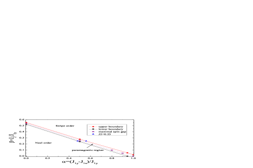
Figure 10: (color online) Phase diagram for the anisotropic $J_{1}$-$J_{2}$ model determined by DMRG. The Néel order and stripe order phases are separated by a paramagnetic regime with the boundaries denoted by the red line with full circles for the upper and the blank line with full squares for the lower transition points, respectively. In the middle of the paramagnetic region lies in a dotted line with crosses which marks the maximal spin-1 gap $\Delta E_{\mathrm{max}}$. Note that the symbols of circle, square, and triangular denote the phase transition points determined by DMRG in the previous figures.

IV Discussion

In summary, we have studied the frustrated spin-1 Heisenberg $J_{1x}$-$J_{1y}$-$J_{2}$ model on a square lattice numerically using the DMRG method and analytically employing the Schwinger-Boson mean-field theory (SBMFT). Interestingly, this model contains both the isotropic $J_{1}$-$J_{2}$ model as well as decoupled Haldane spin chains as limiting cases. Moreover, it has attracted a lot of attention recently since it has been motivated as an effective model to describe the $(0,\pi)$-magnetism and the low-energy spin-wave excitations of the celebrated novel iron pnictide superconductors. Furthermore it has been suggested that the drastic reduction of magnetic moments to a value of 0.4 $\mu_{B}$ is caused by strong quantum fluctuations in the vicinity of a continuous phase transition. However, to the present day the phase diagram has not been determined yet.

Within both the SBMFT and the DMRG we find that the Néel phase is stabilized considerably by quantum fluctuations above the classically stable region up to a relatively strong anisotropy between the NN couplings. However, in all other regards the phase diagrams obtained by the two methods clearly disagree, indicating the importance of the strong quantum fluctuations.

The SBMFT suggest a fluctuation induced first order transition between the Néel and the stripe antiferromagnets terminating at a tricritical point and splitting into two second order lines separated by an intermediate paramagnetic region only for large anisotropies. Although the existence of a tricritical point and a hardly seizable paramagnetic strip terminating at the decoupled Haldane spin chain point ($J_{1x}=J_{2}=0$) are consistent with a recent coupled cluster calculationBishop et al. (2008), the SBMFT definitely falls short on approaching the Haldane chain limit. This becomes clear by a comparison with quantum Monte Carlo simulationsKim and Birgeneau (2000); Matsumoto et al. (2001); Alet and Sorensen (2002) showing a much larger region of stability of the Haldane chain phase against interchain couplings $J_{1x}$. Also the previous two-step DMRG calculationMoukouri (2006) at $J_{1x}/J_{1y}=0.2$ indicates a paramagnetic region being an order of magnitude wider than found within the SBMFT.

On the contrary, the phase diagram obtained within DMRG by a careful finite size scaling of the magnetic structure factor and the spin gap is consistent with both the QMC and the previous DMRG results. Furthermore the spin gap in the decoupled chain limit agrees well with the exact value for the isolated Haldane chain. The width of the paramagnetic region slightly decreases on approaching the isotropic point but remains finite over the entire parameter range. This has the remarkable implication that the paramagnetic phase of the frustrated two dimensional spin model, including the isotropic $J_{1}$-$J_{2}$ limit, is continuously connected to the Haldane spin-chain phase. In other words, the paramagnetic phase can be viewed as a continuation of the Haldane spin chain phase, with the caveat that the topological string order has to disappear at any finite interchain couplingTodo et al. (2001); Anfuso and Rosch (2007).

The reason for the failure of the semiclassical SBMFT in dealing correctly with the strong quantum fluctuations in the boundary region between the two classical orders is easy to understand. The SBMFT deals with the spin as continuous variable while it is blind for the Berry phase effects that distinguish between half-integer and integer spin values crucial for the existence of the Haldane gap as well the valence bond crystals. This physics is definitely missed by the semiclassical treatment. Our DMRG results demonstrates that the Haldane chain phase is very robust against the simultaneous increase of the couplings $J_{1x}$ and $J_{2}$ along the strongly frustrated boundary region, indicated by the minute reduction of the spin gap compared to the isolated Haldane chain limit.

What does the study of this spin system teach us regarding the superconductivity in the iron pnictides? One could speculate that the basic physics is similar as in the cuprates. Although the spins are larger in the pnictides, the geometrical frustration renders the spin system to be on the verge of undergoing a quantum phase transition in a quantum disordered state. This quantum spin physics then sets the conditions for the emergence of superconductivity in the doped systems. But in this regard the size of the microscopic spin does matter more than one intuitively anticipates. For $S=1/2$ the well established fact that the Berry phases conspire to turn the quantum disordered states of the spin-only systems into valence bond solids gives a rationale to take Anderson’s resonating valence bond (RVB) idea for the origin of high Tc superconductivity quite seriously. The valence bonds are protected by the spin gap and the effect of doping could well be to just turn the valence bond solids into translational quantum liquids that transport two units of electrical charge. Focussing on the Berry phases in the pnictides one has only the options of an ‘intermediate’ crystal field $S=1$ stateKrüger et al. (2008) or the high spin $S=2$ for the microscopic spin. In the former case the ground state has a twofold degeneracy and the ‘building blocks’ are no longer pair singlets but instead the ‘chain singlets’. Thinking along the RVB lines, what to expect when such a system is doped? The dopants will increase the quantum fluctuations but chains are not pairs. One anticipates that doping might drive the system into the non-magnetic ‘Haldane chain phase’ breaking the two-fold rotational symmetry of the lattice. One notices that something of the kind is found in the phase diagram of the pnictides: the structural transition to the orthorombic phase persists to much higher dopings than the stripe antiferromagnetismZhao et al. (2008b). At first view this seems rather detached from the RVB idea. But now one has to realize that the charge carriers are themselves spinfull, carrying by default a half-integer spin. Taking for instance the intermediate $S=1$ background, the holes would carry $S=1/2$, and t-J models corresponding with a mix of $S=1$ and $S=1/2$ states have been studied in the pastZaanen et al. (1992). One anticipates that in an incompressible ‘chain like’ $S=1$ background the $S=1/2$ carriers might again be ‘glued by Berry forces’ into valence bond pairs, re-establishing a connection with the RVB mechanism of the cuprates. A similar idea has been previously proposed from a different approachBaskaran (2008).

In conclusion, it is quite questionable that any of these considerations have a bearing on pnictide superconductivity but they do make the case that there is still much interesting physics to be explored dealing with systems characterized by a larger microscopic spin.

Acknowledgment: We are grateful for stimulating discussion with M. Q. Weng. This work is partially supported by NSFC and the National Program for Basic Research of MOST, China, the DARPA OLE program, the DOE grant DE-FG02-06ER46305, the NSF grant DMR-0605696 and the Stichting voor Fundamenteel Onderzoek der Materie (FOM).

References

- Kamihara et al. (2008) Y. Kamihara, T. Watanabe, M. Hirano, and H. Hosono, J. Am. Chem. Soc. 130, 3296 (2008).
- Takahashi et al. (2008) H. Takahashi, K. Igawa, A. Kazunobu, and Y. Kamihara, Nature (London) 453, 376 (2008).
- Ren et al. (2008) Z. A. Ren, J. Yang, W. Lu, W. Yi, G. C. Che, X. L. Dong, L. L. Sun, and Z. X. Zhao, Materials Research Innovations 12, 105 (2008).
- Chen et al. (2008a) X. H. Chen, T. Wu, G. Wu, R. H. Liu, H. Chen, and D. F. Fang, Nature (London) 453, 761 (2008a).
- Chen et al. (2008b) G. F. Chen, Z. Li, D. Wu, G. Li, W. Z. Hu, J. Dong, P. Zheng, J. L. Luo, and N. L. Wang, Phys. Rev. Lett. 100, 247002 (2008b).
- de la Cruz et al. (2008) C. de la Cruz, Q. Huang, J. W. Lynn, W. R. J. Li, J. L. Zarestky, H. A. Mook, G. F. Chen, J. L. Luo, N. L. Wang, and P. Dai, Nature (London) 453, 899 (2008).
- Yao and Carlson (2008) D.-X. Yao and E. W. Carlson, Phys. Rev. B 78, 052507 (2008).
- Zhao et al. (2008a) J. Zhao, D.-X. Yao, S. Li, T. Hong, Y. Chen, S. Chang, W. R. II, J. W. Lynn, H. A. Mook, G. F. Chen, et al., Phys. Rev. Lett. 101, 167203 (2008a).
- McGuire et al. (2008) M. A. McGuire, A. D. Christianson, A. S. Sefat, B. C. Sales, M. D. Lumsden, R. Jin, E. A. Payzant, D. Mandrus, Y. Luan, V. Keppens, et al., Phys. Rev. B 78, 094517 (2008).
- Krüger et al. (2008) F. Krüger, S. Kumar, J. Zaanen, and J. van den Brink (2008), URL arXiv.org:0811.4104.
- Xu et al. (2008) C. Xu, M. Muller, and S. Sachdev, Phys. Rev. B 78, 020501(R) (2008).
- Fang et al. (2008) C. Fang, H. Yao, W.-F. Tsai, J. P. Hu, and S. A. Kivelson, Phys. Rev. B 77, 224509 (2008).
- Chandra and Doucot (1988) P. Chandra and B. Doucot, Phys. Rev. B 38, 9335 (1988).
- Xu and Ting (1990) J. H. Xu and C. S. Ting, Phys. Rev. B 42, 6861 (1990).
- Gochev (1995) I. G. Gochev, Phys. Rev. B 51, 16421 (1995).
- Mila et al. (1991) F. Mila, D. Poilblanc, and C. Bruder, Phys. Rev. B 43, 7891 (1991).
- Krüger and Scheidl (2006) F. Krüger and S. Scheidl, Europhys. Lett. 74, 896 (2006).
- Dagotto and Moreo (1989) E. Dagotto and A. Moreo, Phys. Rev. Lett. 63, 2148 (1989).
- Schulz and Ziman (1992) H. J. Schulz and T. A. L. Ziman, Europhys. Lett. 18, 355 (1992).
- Schulz et al. (1996) H. J. Schulz, T. A. L. Ziman, and D. Poilblanc, J. Phys. I 6, 675 (1996).
- Sindzingre (2004) P. Sindzingre, Phys. Rev. B 69, 094418 (2004).
- Capriotti and Sorella (2000) L. Capriotti and S. Sorella, Phys. Rev. Lett. 84, 3173 (2000).
- Capriotti et al. (2001) L. Capriotti, F. Becca, A. Parola, and S. Sorella, Phys. Rev. Lett. 87, 097201 (2001).
- Gelfand et al. (1989) M. P. Gelfand, R. R. P. Singh, and D. A. Huse, Phys. Rev. B 40, 10801 (1989).
- Gelfand (1990) M. P. Gelfand, Phys. Rev. B 42, 8206 (1990).
- Singh et al. (1999) R. R. P. Singh, Z. Weihong, C. J. Hamer, and J. Oitmaa, Phys. Rev. B 60, 7278 (1999).
- Sushkov et al. (2001) O. P. Sushkov, J. Oitmaa, and Z. Weihong, Phys. Rev. B 63, 104420 (2001).
- Sushkov et al. (2002) O. P. Sushkov, J. Oitmaa, and Z. Weihong, Phys. Rev. B 66, 054401 (2002).
- Bishop et al. (1998) R. F. Bishop, D. J. J. Farnell, and J. B. Parkinson, Phys. Rev. B 58, 6394 (1998).
- Read and Sachdev (1989) N. Read and S. Sachdev, Phys. Rev. Lett. 62, 1694 (1989).
- Read and Sachdev (1990) N. Read and S. Sachdev, Phys. Rev. B 42, 4568 (1990).
- Sachdev (2008) S. Sachdev, Nature Physics 4, 173 (2008).
- Bishop et al. (2008) R. F. Bishop, P. H. Y. Li, R. Darradi, and J. Richter, Europhys. Lett. 83, 47004 (2008).
- Moukouri (2006) S. Moukouri, Phys. Lett. A 352, 256 (2006).
- Sorensen and Affleck (1993) E. S. Sorensen and I. Affleck, Phys. Rev. Lett. 71, 1633 (1993).
- Haldane (1983a) F. D. M. Haldane, Phys. Lett. A 93, 464 (1983a).
- Haldane (1983b) F. D. M. Haldane, Phys. Rev. Lett. 50, 1153 (1983b).
- Todo et al. (2001) S. Todo, M. Matsumoto, C. Yasuda, and H. Takayama, Phys. Rev. B 64, 224412 (2001).
- Anfuso and Rosch (2007) F. Anfuso and A. Rosch, Phys. Rev. B 76, 085124 (2007).
- denNijs and Rommelse (1989) M. denNijs and K. Rommelse, Phys. Rev. B 40, 4709 (1989).
- Kim and Birgeneau (2000) Y. J. Kim and R. J. Birgeneau, Phys. Rev. B 62, 6378 (2000).
- Matsumoto et al. (2001) M. Matsumoto, C. Yasuda, S. Todo, and H. Takayama, Phys. Rev. B 65, 014407 (2001).
- Alet and Sorensen (2002) F. Alet and E. S. Sorensen, Phys. Rev. B 65, 092408 (2002).
- Zinke et al. (2008) R. Zinke, J. Schulenburg, and J. Richter, Eur. Phys. J. B 61, 147 (2008).
- Cai et al. (2007) Z. Cai, S. Chen, S. Kou, and Y. Wang, Phys. Rev. B 76, 054443 (2007).
- R.White (1992) S. R.White, Phys. Rev. Lett 69, 2863 (1992).
- Zhao et al. (2008b) J. Zhao, Q. Huang, C. de la Cruz, S. Li, J. W. Lynn, Y. Chen, M. A. Green, G. F. Chen, G. Li, Y. Li, et al., Nature Materials 7, 953 (2008b).
- Zaanen et al. (1992) J. Zaanen, A. M. Oles, and P. Horsch, Phys. Rev. B 46, 5798 (1992).
- Baskaran (2008) G. Baskaran (2008), URL arXiv.org:0804.1341.