The Evolution and Decay of Supersymmetric Flat Directions in the Early Universe and Their Role in Thermalizing the Universe

Abstract

I study the post-inflation oscillation and decay of light coherent scalar field condensates that may develop during an inflationary phase of the universe. In particular, the light scalars studied are a composition of the scalar particles of a supersymmetric theory which correspond to the flat directions of the theory’s scalar potential. Some toy models that possess supersymmetric flat directions are presented and numerical solutions for the evolution of the scalar fields are obtained. Both analytic and numeric results suggest that such condensates, if they existed in the early universe, can decay through a rapid and nonperturbative process long before these condensates could significantly affect the thermalization of the universe.

University of Minnesota Physics Prof. Marco Peloso

December 2008

I would like to thank my Adviser Marco Peloso who I worked closely with on much of the material presented here and who provided invaluable suggestions and comments. I would also like to thank A. Emir Gümrükçüoğlu and Professor Keith Olive who also worked on these problems and who contributed helpful comments and suggestions. Finally, I would like to thank the other members of my Dissertation committee; Professors John Wygant, Joseph Kapusta, and Dan Cronin-Hennessey for their time and helpful comments. This work is dedicated to my wife Dohi, to our boys Owen and Ryan and to our parents whose encouragement made this work possible.

Chapter Introduction

Inflation and Supersymmetry are central topics in modern cosmology and modern particle physics. There is indirect evidence in support of inflation [1], and there is theoretical and phenomenological motivation for supersymmetry [3]. This thesis is devoted to some problems in early universe cosmology assuming both inflation and low energy supersymmetry are a part of nature. The discussion will be of the dynamics of coherent scalar fields in the early universe and their possible effects on Cosmology. One coherent scalar field to be reviewed is the inflaton which is the proposed field responsible for inflation. The other scalars, which are the focus of the work, are those of a supersymmetric theory such as the Minimal Supersymmetric Standard Model (MSSM). These fields may have been prepared in a coherent state through the process of inflation. Our goal is to obtain an order of magnitude estimate for the decay (or decoherence) time of these coherent scalar fields after the conclusion of the inflation.

It is worthwhile to briefly consider the larger context of fundamental scalar fields in nature. Scalar fields are associated with many strange effects in particle physics and cosmology. For example, the Higgs Mechanism, which is believed to be responsible for Electroweak symmetry breaking, is mediated by a fundamental scalar Higgs field(s). Also, inflation is believed to be due to the evolution of a coherent scalar field called the inflaton. Similarly, the present observed acceleration of the universe [8] may be caused by the dynamics of a scalar field called quintessence [9]. While composite scalar fields (bound states) have been observed, not one fundamental scalar field has ever been observed. All the observed fields of the standard model of particle physics are spin 1/2 fermions or vector gauge bosons. The yet to be observed Higgs boson is in fact the only fundamental scalar field in the standard model. One possibility is that fundamental scalars simply do not exist in nature. For instance, there exist well motivated models of particle physics which allow for Electroweak symmetry breaking without a fundamental scalar Higgs field [10]. However, there appears to be no a priori reason to disallow fundamental scalars, and on the contrary, nature may be signaling their existence in the above examples.

Scalar fields also possess peculiar classical and quantum mechanical properties. For instance, without some protective mechanism, the effective masses of scalar fields are not stable to quantum corrections and they will run up to the fundamental scale of ones theory which is typically the Planck scale $M_{P}\sim 10^{19}\,\mathrm{GeV}$ or the Grand Unification Scale $M_{GUT}\sim 10^{16}\,\mathrm{GeV}$. This sensitivity to the ultraviolet scale is one aspect of what is commonly known as the Hierarchy problem. The second aspect to the Hierarchy problem is why these scales should be so much larger than the scale of Electroweak symmetry breaking which is of order $\mathrm{TeV}$. We do not attempt to explain the Hierarchy of scales here, but this Hierarchy, which amounts to thirteen or sixteen orders of magnitude, will in fact play a role in our models and analyses.

A second peculiar property of scalar fields is that they may obtain a uniform classical Vacuum Expectation Value (VEV) over all the observable universe. The above three examples of the Higgs mechanism, inflation, and quintessence are all essentially consequences of this property that scalar fields may obtain a VEV. Other fields such as the gravitational field and gauge vector fields may obtain Vacuum Expectation Values, but for these to be uniform over our observable universe implies a preferred direction to space, or could be simply reinterpreted as a scalar component to these fields (in the case of cosmological perturbations for instance). Vector and tensor fields can be classical on local scales of course, as in a laser or in the gravitational fields of stars and planets. Only a scalar field can possess a Lorentz invariant vacuum expectation value which would be essentially unobservable except for its modification of fundamental properties of nature. Specifically, in the Higgs mechanism, the Lorentz invariant scalar Higgs VEV couples to the leptons and quarks of the standard model in such a way to give them the effective masses that we measure in the laboratory. The proposed inflaton evolved in time and thus broke Lorentz invariance; however, it was a uniform VEV over a large patch of space which resulted in a largely uniform energy density and temperature in the early universe. The remnants of this uniform bath are observable today as the nearly perfect thermal spectrum of the cosmic microwave background [11]. The concept of a vacuum expectation value of a scalar field is so fundamental to modern particle theories, that when it arises in a model, it is simply referred to as “the” vacuum of the model.

The first property mentioned above of the instability of the scalar field’s mass to quantum corrections can be corrected by making ones theory supersymmetric which cancels the instability and allows for a hierarchy of scales to be phenomenologically viable. Note that supersymmetry does not explain why the hierarchy is there however. The second property mentioned is a generic property of bosonic fields that they may coalesce into a Bose-Einstein condensate. To understand how such VEVs can develop in nature, it is unavoidable to look to cosmology for guidance.

The theory of inflation proposes that there was a stage during the early universe in which space stretched at an accelerated rate. If the inflation was exponential, the line element would be written $ds^{2}=dt^{2}-e^{2Ht}d{\vec{x}}^{2}$. This inflation ended when the agent which was responsible for the acceleration had spent enough of its energy into the expansion that the exponential expansion could no longer continue. If one neglects quantum effects during inflation, then all other species of particles are diluted to negligible amounts by the inflation, with the only remaining constituent to the energy density being the inflaton. The model of inflation solved a few outstanding problems of cosmology at the time it was conceived [12], and other useful models of inflation were soon developed [13, 14]. The model of chaotic inflation [14] is the one which will be applied here.

A first ingredient to our study is the fact that inflation can magnify the quantum fluctuations of a field into an observable classical wave with non-negligible energy density. It may be shown in particular that this happens to scalar fields whose mass is sufficiently small [15]. This effect on the quantum fluctuations of a field is actually a generic property of all inflation models because it is an effect of the accelerated expansion itself. Specifically, all that is required is a small enough event horizon during inflation for the fluctuations to propagate past and become frozen [16]. The event horizon during inflation is approximately the inverse Hubble parameter $H^{-1}$ which can be as small as $10^{-30}$ meters in many inflation models. It is not so unbelievable to imagine a quantum fluctuation propagating over such a short distance. Finally, it is noted that this effect of inflation on the quantum fluctuations of a field is believed to be the source of the cosmological perturbations [17] which has left a signature in the large scale structure of the universe [18] and in the Cosmic Microwave Background [19]. While the study of the cosmological perturbations is a central theme in cosmology, it will not be the focus of this work.

The second ingredient to our study is that supersymmetry and the MSSM in particular provides many such light scalar fields. If inflation lasted a long enough time, then some set of these scalar fields would have obtained non-negligible VEVs by the conclusion of inflation through the above effect on their quantum fluctuations. Such scalar field VEVs may then have implications for cosmology. For instance, one beneficial feature of these scalar field VEVs is their potential to contribute to baryogenesis [20]. There may also be adverse effects from light scalar field VEVs in the early universe, and these will be discussed shortly.

The scalar fields we are interested in are the scalar particles of the MSSM. In general, these fields are coupled to one another, and if during inflation any one of these begin to obtain a VEV, it will induce an effective mass in the other fields it couples to. It may even induce an effective mass to itself through quartic self-interactions of the MSSM. To see this, one may expand the field as $\phi=\Phi+\delta\phi$ where $\Phi$ is the VEV (to be treated classically) and $\delta\phi$ are the quantum fluctuations. Considering a potential such as $V=m^{2}|\phi|^{2}+\lambda|\phi|^{4}$ and expanding in $\delta\phi$, the mass term of the perturbations may be extracted. Schematically, one obtains,

$$m^{2}|\phi|^{2}+\lambda|\phi|^{4}\rightarrow(m^{2}+\lambda\Phi^{2})\delta\phi^{2}$$ (1)

Then assuming the bare mass $m$ is small (specifically $m<H$), and assuming inflation lasts a sufficiently long time, the VEV $\Phi$ will accumulate during inflation, and the above effective mass of the perturbations will grow. In some patches of the universe, the effective mass may grow to exceed $m$ and become comparable to $H$. After this instant, the growth of the VEV in these patches will stop. In this way, the interaction terms of the scalar potential in the MSSM can suppress the growth of VEVs during inflation to be orders of magnitude below the Planck mass. However, in the MSSM and other supersymmetric theories, there are special combinations of the scalar fields for which the renormalizable potential is exactly zero! These are known as supersymmetric flat directions. The flat directions are tilted slightly by supersymmetry breaking masses $m\sim\mathrm{TeV}$, but these masses are small compared to the Hubble parameter during inflation which can be $10^{13}\,\mathrm{GeV}$ in many models. In this case, assuming there are no other higher order Planck suppressed interactions in the scalar potential, and assuming inflation lasts a relatively long time, the scalar field VEV can become larger than $M_{P}$. Because the mass is small, the energy density of these VEVs should still remain below that of the inflaton during inflation. However, after inflation has ended and after the inflaton condensate has decayed, there are scenarios in which the energy density of the light scalar fields can in fact overtake that of the inflaton’s decay products. One potential adverse effect of such scenarios is that if the light scalars possess a baryonic or leptonic charge, as in the Affleck-Dine mechanism [20], they could yield an overly large baryon asymmetry [20, 21]. Additionally if the scalars dominate the inflaton, their fluctuations will be the cosmological perturbations, and then ones modeling must be sensitive to the associated phenomenological constraints from the CMB (see [22] and references there in).

The above problem of a flat direction field coming to dominate the energy density of the universe is one example of a generic problem in reconciling many extensions of the standard model with inflationary cosmology. It is known as the moduli problem. The problem is that weakly interacting light fields with large enough energy density may persist in the universe for an extended period of time and may upset the successful predictions of the big bang cosmology. For instance if the fields decay late, they may generate too much entropy and result in an unacceptably small baryon asymmetry [23, 24] or they may upset the the predictions of nucleosynthesis [24]. Alternatively, if these fields are stable, they may provide too much dark matter to be consistent with observation such as in the case of the gravitino problem to be discussed shortly.

However, there can be benefits of having flat direction VEVs. One benefit is the mechanism of baryogenesis mentioned earlier [20]. Another possible benefit is a lower reheating temperature [25], but this benefit may be difficult to realize [26, 27], and why this is the case will be reviewed shortly. In general, the cosmological effects of flat directions depend strongly on the evolution of the inflaton and flat direction fields during the post-inflation phase of the universe but before the thermal phase. This is the phase of thermalization or “reheating” as it is commonly known and we shall briefly discuss this. After inflation has ended, the inflaton dominates the energy density of the universe, and it will be mostly uniform over large patches of space, but it will oscillate in time and otherwise behave as a condensate of massive zero momentum particles in any particular patch. It will decay by some unknown mechanism into the quanta of the standard model or of MSSM or of some other extension of the standard model. The reheating temperature mentioned above is simply the temperature achieved by the inflaton’s decay products once they have thermalized. The reheating temperature can also be loosely thought of as the highest temperature that the universe ever reached.

An upper bound for the reheating temperature is determined by the energy density of the inflaton at the conclusion of inflation if one assumes that decay and thermalization happen instantly at this time. The energy density at this time is related to the Hubble parameter through the Friedmann equation, and measurements of the CMB put a bound on the Hubble parameter at the end of inflation of about $H_{I}<10^{15}\,\mathrm{GeV}$. From this, a bound on the reheating temperature $T_{RH}<10^{16}\,\mathrm{GeV}$ is obtained (see Section The Evolution and Decay of Supersymmetric Flat Directions in the Early Universe and Their Role in Thermalizing the Universe). At the opposite extreme, the reheating temperature must be greater than a MeV because nucleosythesis happens at this temperature and requires a thermal bath. Thus, there is approximately 19 orders of magnitude of uncertainty in the reheating temperature. However, we note that in most models, the reheating temperature is significantly lower than the above upper bound to account for a finite decay time of the inflaton. To summarize, both $H_{I}$ and $T_{RH}$ are two important benchmarks for a cosmological model as both quantities set the energy scale for the physical processes which may occur. For instance, one successful feature of inflation is that it can dispose of dangerous heavy relic particles or topological defects such as magnetic monopoles which are prevalent in Grand Unified theories and also generated in large quantities at GUT scale temperatures [12]. Such particles are disposed of by the effect of dilution. Inflation thus solves the monopole problem, but there are other heavy relics which can be generated thermally and perhaps non-thermally after inflation has ended. If the reheating temperature is higher than about $10^{6}-10^{9}\,\mathrm{GeV}$ then one such hypothetical heavy particle, the gravitino, can be produced in large enough quantities to either upset the predictions of nucleosynthesis, or if the gravitino is stable, provide too much dark matter [28, 29, 30]. Thus, there is incentive for cosmologists to construct models with naturally lower reheating temperatures. A simple and well motivated mechanism to lower the reheating temperature is if the inflaton decays through Planck suppressed interactions, here referred to as a gravitational decay. The reheating temperature is then restricted to be below approximately $10^{9}\,\mathrm{GeV}$ which is still not quite enough to prevent the above mentioned gravitino problem [28, 29, 30]. The reheating temperature may be further reduced if the interactions which thermalize the inflaton decay products are somehow suppressed. These interactions would presumably be gauge interactions, and a simple mechanism for suppressing them is if the gauge bosons which mediate the interactions have acquired large masses [20, 25]. In fact, the flat direction VEVs just discussed can provide this mechanism because the VEVs typically break many or all of the standard model gauge symmetries [31, 32]. The effective vacuum established will then consist of heavy gauge vector bosons among other heavy states. This would indeed suppress the thermalizing interactions and it could lower the reheating temperature as mentioned above. However, to obtain a significant suppression, it requires the flat directions to remain coherent over a long time and in such cases the flat direction’s energy density may come to dominate over that of the inflaton [26, 33]. Flat direction domination can be problematic as discussed above.

The suppression of thermalization depends on the flat direction VEVs remaining coherent over a relatively long time, and this has spurred a recent discussion over the time scale for the decay of flat direction VEVs [25, 26, 27, 34, 35, 36, 37, 38, 39] of which this thesis is a part. A perturbative estimate of the decay rate of the flat direction VEVs support the hypothesis of a long lived flat direction [25], but this estimate clearly depends on the VEVs remaining coherent. The VEVs will decay eventually, putting the universe back into the gauge symmetric state, but until the decay, the vacuum is in the broken state discussed above. However the vacuum is also evolving – so strictly speaking it is not a vacuum – and it has been pointed out in [26] that the evolution may in fact be non-adiabatic. The time scale of the evolution is long compared to the fast (heavy) scales such as the oscillation of the inflaton. In this sense it is a good approximation to treat the background VEVs as a vacuum. However, the flat direction VEVs typically possess more than one complex degree of freedom, and the relative evolution of these light degrees of freedom can be a source of non-adiabatic evolution. The corresponding light quanta to the flat direction degrees of freedom are thus not necessarily adiabatically invariant. The argument along the above lines is proposed and developed in [26, 27], and the results indicate that non-adiabatic evolution may contribute to flat direction decay. Much of the new material presented in this thesis is based on the work of [27] and also extends and clarifies some of these results. In the remainder of the introduction, this work is described.

The decay of the flat directions can equivalently be described as the onset of spatial instability to the flat direction condensates. Like the inflaton, the flat direction VEVs can be treated as condensates of massive zero momentum scalar particles, but with masses approximately $10^{10}$ times smaller than that of the inflaton. The decay of the condensates proceeds by “kicking” quanta from the zero momentum modes into higher momentum states through the effect of the non-adiabatically evolving background. In position space, this simply corresponds to the development of spatial instability of the condensate.

If the condensate is perfectly uniform over space and if all fields are treated classically, a spatial instability will not develop. However, one expects there to be small noise fluctuations on top of the uniform field. Even assuming the absence of classical noise, there is quantum noise, and the dynamics of the uniform field is not necessarily stable to either source of noise. Specifically, both classical and quantum noise can be amplified by the effect of the evolving background which couples to the noise perturbations through effective and time dependent mass terms. The instability is thus produced by parametric resonance.

The formalism here used to quantify the above instability is that of quantum fields in external backgrounds, and it is commonly used in quantum field theory and cosmology [40]. It is typically applied to handle the case of a single field with a time dependent frequency. The formalism was extended to handle multiple scalar and fermionic fields in [41] and it is further developed for scalars here. As an example of these new developments, consider in the single field analysis, the quantity $\dot{\omega}/\omega^{2}$. Specifically, one indication of nonadiabatic evolution is when the frequency of a state changes in a time comparable to or faster than one period of oscillation for the state, or $\dot{\omega}/\omega^{2}\raisebox{-0.43057pt}{ $\begin{array}[]{@{}c}\scriptstyle>\\ \scriptstyle\sim\end{array}$}1$. This measure of non-adiabatic evolution is here generalized to the case of multiple scalar fields where one must not only keep track of the time evolution of the eigenfrequencies, but also the time evolution of the eigenvectors. In particular, if any eigenvector has changed during a time comparable to or greater than the oscillation period of any state of the system, the evolution can be non-adiabatic. These quantities can thus be arranged in a matrix. The matrix expression is relatively simple and is presented here and in [27], but to our knowledge has not been reported elsewhere. As in the single field case, the elements of this matrix provide a convenient preliminary measure of non-adiabatic evolution. They are applied in this thesis for this specific purpose.

An alternative method for studying the spatial instability of the flat directions, which contrasts to the above formalism, is the lattice simulation of the classical field theory [42]. Such classical simulations are possible when the condensates have large occupation numbers. For instance, lattice methods have been performed successfully to study nonperturbative decay of the inflaton condensate [43]. Lattice methods may in principle also be applied to study flat directions but there are no published examples to date. However as these simulations are very demanding with respect to computer memory, the types of models that can be studied are thus limitted. The methods used here are more amenable to analytic arguments, are less computationally demanding than lattice methods, and these methods also incorporate quantum effects by construction. Lattice methods are not applied in this work, but have not been ruled out for future work.

One limitation to our formalism is that it is performed at quadratic order in the perturbations. Interaction terms are not included, and also the production of quanta is not reflected by a corresponding depletion of the evolving flat direction condensate. Our models strictly do not conserve energy in this respect and thus become unreliable when the energy density of the produced quanta becomes comparable to the energy density in the flat direction VEVs. However, the formalism is known to adequately model the initial phase of exponential particle production. For instance, a comparison of the two methods for a toy inflation model has been found in qualitative agreement [44]. Our goal is to obtain an order of magnitude estimate of the VEV’s decoherence (decay) time, and by determining the initial growth exponent, this goal may be achieved. The effects of interactions will be discussed at the conclusion of Section The Evolution and Decay of Supersymmetric Flat Directions in the Early Universe and Their Role in Thermalizing the Universe.

Another important aspect to studying the decay of flat directions which is developed here is the handling of the gauge symmetry. Due to the complexity involved in studying flat directions with the full $SU(3)\times SU(2)\times U(1)$ standard model gauge group, only $U(1)$ gauge models are here presented. Despite this limitation, our analysis correctly handles the gauge fixing of the perturbations and in particular the vector longitudinal modes (Goldstone mode) which do not necessarily decouple from the other scalar perturbations. Choosing the unitary gauge is the most convenient choice and once this gauge is fixed, the constraints of gauge current conservation become transparent. We show how the constraints of current conservation lead to non-trivial consequences for the evolution of the flat direction VEVs.

We apply the above gauge fixing to two simple $U(1)$ models involving both a single flat direction and also multiple flat directions [26]. The multiple flat direction model will be shown to yield non-adiabatic evolution. One expects the perturbations to the flat direction VEVs to also be the states involved in the non-adiabatic evolution because these are the light states of the vacuum and so evolve on the same time scale as the vacuum. To understand why the model can lead to a parametric resonance, one first tabulates the degrees of freedom. The multiple flat direction model consists of the gauge vector and four charged complex scalars. The time-like component of the vector is non-dynamical so this removes one degree of freedom, and the gauge fixing removes a second degree of freedom. There remains ten propagating physical degrees of freedom. Three of these degrees of freedom will belong to the massive vector and one will belong to a heavy Higgs state of the same mass as the vector. There remains six light degrees of freedom, and these necessarily correspond to three flat direction degrees of freedom of the model. However not all of the flat directions necessarily obtain VEVs, and in the solutions we consider, the gauge current constraint mentioned above allows only two of the three flat directions to obtain a VEV. The remaining flat direction which did not obtain a VEV mix with the Higgs perturbation and this system of three real fields mixes strongly and results in parametric resonance.

It will be shown that all three states including the heavy Higgs will be produced in the resonance. It will also be found that the production of the heavy states compared to that of the two light quanta is consistent with the principle of equipartition of the energy. The equipartition here will not be that of a thermal bath, but rather a property of the strong coupling between the modes, and more akin to the equipartition seen in some classical systems of strongly coupled oscillators [45, 46]. The equipartition observed in the numeric results is also obtained by direct analysis of the Heisenberg equations of motion from which a scaling property of these equations is obtained. In particular, this scaling allows us to rescale our numerical solutions, which are limited by machine precision to a small hierarchy of approximately nine orders of magnitude to the phenomenologically relevant case in which the hierarchy is up to sixteen orders of magnitude.

The numeric results of this thesis will suggest that a system of multiple flat directions can decay nonperturbatively for a broad range of parameters via parametric resonance. Numerical estimates of the decay time will be part of these results. In addition to the numeric results, some formal results stand on their own. In particular the scaling arguments, the adiabaticity parameters, the reformulation of the Heisenberg equations of motion (not mentioned above), and the gauge fixing procedure are all new results, and potentially useful tools in further study.

The plan of the thesis is as follows: In Section The Evolution and Decay of Supersymmetric Flat Directions in the Early Universe and Their Role in Thermalizing the Universe, we lay out the formalism for identifying and cataloguing of MSSM flat directions. This includes a motivation of the scalar potential (the D and F terms) of the MSSM, the formalism of gauge invariant monomials for identifying flat directions, and the lifting of flat directions by the nonrenormalizable superpotential. This section concludes with a brief discussion of supersymmetry breaking, and the spectrum of soft sparticle masses.

In Section The Evolution and Decay of Supersymmetric Flat Directions in the Early Universe and Their Role in Thermalizing the Universe we discuss the formalism for describing the quantum evolution of a system of coupled scalar fields in a time dependent background, or the Heisenberg equations of motion. In particular we continue the program begun in [41] by presenting some new formal tools and discussing the solution of the Heisenberg equations when there is a hierarchy of mass scales. We also draw the connection between the evolution and an equipartition of energy.

In Section The Evolution and Decay of Supersymmetric Flat Directions in the Early Universe and Their Role in Thermalizing the Universe a brief introduction to classical inflation is presented followed by a description of the mechanism by which quantum fluctuations of light scalar field such as the SUSY flat directions will be converted into a VEV through inflation. We discuss the post-inflation evolution of the VEVs and the likelihood of obtaining large VEVs of order the Planck Mass.

Section The Evolution and Decay of Supersymmetric Flat Directions in the Early Universe and Their Role in Thermalizing the Universe contains discussion of different scenarios for reheating but is focused on a standard case in which the bulk of the produced entropy is from the inflaton. In our discussion of reheating, we emphasize nonperturbative dynamics or “preheating” scenarios as they are known in the literature. The calculation of the reheating temperature and the baryon asymmetry is discussed. The potential effects of flat directions on the reheating process is also discussed

In Section The Evolution and Decay of Supersymmetric Flat Directions in the Early Universe and Their Role in Thermalizing the Universe we explain the procedure for gauge fixing a generic model of U(1) flat directions to the unitary gauge. We then apply the procedure to two simple U(1) symmetric models of flat directions, and we calculate the formal expressions which describe the non-perturbative decay of one of the models.

In Section The Evolution and Decay of Supersymmetric Flat Directions in the Early Universe and Their Role in Thermalizing the Universe the multiple flat direction model is solved numerically and the results for the production of quanta is presented. A useful scaling relation is described which allows us to rescale our results from an energy scale dictated by limitations of the computer to the much smaller Electroweak scale masses that are phenomenologically relavant.

We conclude in Section The Evolution and Decay of Supersymmetric Flat Directions in the Early Universe and Their Role in Thermalizing the Universe with some discussion of the implications of our results, and in particular which features may be generically applicable to the MSSM. We also indicate future directions of study.

In the Appendix, a brief discussion of the notation of the thesis is provided, as well as some calculations too lengthy to show in the main text.

Chapter Supersymmetry and Flat Directions of the Scalar Potential

In this section, we present a brief introduction to supersymmetric field theory in order to motivate the scalar potential in these theories, and the “flat directions” which are the minima of the scalar potential. We describe the methods for identifying flat directions of a supersymmetric theory which involve gauge invariant monomials [47]. We then discuss the terms of the superpotential which are expected to lift the flat directions [31, 32], providing a natural cutoff for the VEV a flat direction may obtain during inflation. We conclude with a brief discussion of supersymmetry breaking and the spectrum of soft sparticle masses which also appear in the scalar potential and which characterize the classical evolution of a flat direction during and after inflation. Much of the background material related to supersymmetry was gathered from the review [4].

1 The Lagrangian of a Supersymmetric Field Theory and its Scalar Potential

Below we introduce supersymmetric field theory and the scalar potential in these theories.

A supersymmetry transformation will transform a bosonic field into a fermionic one and vice-versa while preserving the form of the terms in the Lagrangian. For instance, the canonical kinetic terms for a complex spin-0 scalar $\phi$, and that of a two component spin-1/2 fermion $\psi$ in the Lagrangian are

$$\partial_{\mu}\phi^{*}\partial^{\mu}\phi+i\psi^{\dagger}{\bar{\sigma}}^{\mu}\partial_{\mu}\psi$$ (2)

A supersymmetry transformation should have the effect $\{\phi,\psi\}\rightarrow\{\tilde{\phi},\tilde{\psi}\}$ such that the form of the above kinetic terms will have not changed after the transformation. A simpler symmetry which one may compare to supersymmetry, is the symmetry of the following Lagrangian involving two complex scalar fields $\phi_{1}$ and $\phi_{2}$,

$$\partial_{\mu}\phi_{1}^{*}\partial^{\mu}\phi_{1}+\partial_{\mu}\phi_{2}^{*}\partial^{\mu}\phi_{2}-m^{2}(|\phi_{1}|^{2}+|\phi_{2}|^{2})$$ (3)

This Lagrangian is invariant under SU(2) transformations of the doublet $(\phi_{1},\phi_{2})$ which rotates the scalar fields $\phi_{1}$ and $\phi_{2}$ into each-other. The transformation matrix can be written $e^{i\vec{\epsilon}\cdot\vec{\tau}}$ where $\vec{\epsilon}=(\epsilon_{1},\epsilon_{2},\epsilon_{3})$ is a vector specifying the rotation and $\tau=\frac{1}{2}(\sigma_{1},\sigma_{2},\sigma_{3})$ are the group generators. The infinitesimal form of this transformation is,

$$\left(\begin{array}[]{l}\phi_{1}\\ \phi_{2}\end{array}\right)\rightarrow(1+i\vec{\epsilon}\cdot\vec{\sigma})\left(\begin{array}[]{l}\phi_{1}\\ \phi_{2}\end{array}\right).$$ (4)

For example, the standard model Higgs field transforms in this way. A supersymmetry transformation is slightly more involved than an SU(2) transformation however as the generators of the supersymmetry transformation are anti-commuting spinors. Under an infinitesimal supersymmetry transformation a scalar $\phi$ and a fermion $\psi$ will transform via an anti-commuting two component spinor $\epsilon$ as follows,

$$\delta\phi\rightarrow\phi+\epsilon^{\alpha}\psi_{\alpha}\;\;\;,\;\;\;\psi_{\alpha}\rightarrow\psi_{\alpha}+i(\sigma^{\mu}\epsilon^{\dagger})_{\alpha}\partial_{\mu}\phi$$ (5)

where $\alpha=1,2$ indexes the two components of the spinor. This infinitesimal SUSY transformation is to be compared with the infinitesimal $SU(2)$ transformation (4) shown above. There is a further subtlety in the above SUSY transformation that for the transformation to be consistent, it is necessary that the number of bosonic degrees of freedom in $\phi$ match the number of fermionic degrees of freedom in $\psi$. At a cursory level there is a problem since the spinor is described by two complex values while the scalar is described by one complex value. Of course, there are only two on-shell degrees of freedom in both the scalar and spinor, but the other two spinor degrees of freedom can go off-shell when calculating a quantum amplitude, and we will want our transformation to be applicable both on-shell and off-shell. In order to match both the on-shell and off-shell degrees of freedom, a complex auxiliary field $F$ is introduced. This field will not be dynamical. It will be rather a Lagrange multiplier in the classical sense, but it will make up the difference of off-shell degrees of freedom for the scalar so that the fermion may consistently “rotate” into the spin-0 boson. The auxiliary $F$ field is necessary for the supersymmetry transformation to be consistent. The combination of a complex spin-0 scalar $\phi$, a two component spinor $\psi$, and the auxiliary field $F$ is known in the literature as a “chiral multiplet”, and it transforms consistently into itself under supersymmetry transformations. The chiral multiplets have the following form in the Lagrangian,

$$\mathcal{L}_{\mathrm{chiral}}=\partial_{\mu}\phi_{i}^{*}\partial^{\mu}\phi_{i}+i\psi_{i}^{\dagger}{\bar{\sigma}}^{\mu}\partial_{\mu}\psi_{i}+F_{i}^{*}F_{i}+\mathcal{L}_{\mathrm{chiral\;int}}$$ (6)

which is simply the canonical kinetic terms shown previously, plus a quadratic part in the the auxiliary field $F$, plus interactions between multiplets encoded in ${\cal L}_{\mathrm{chiral\;int}}$ to be specified shortly. Every standard model fermion (a quark or lepton) is expected to belong to a “chiral multiplet” such as above, and so is expected to have a spin-0 counterpart (a squark or slepton). Additionally, the as yet to be discovered Higgs sector fields are also expected to belong to chiral multiplets, and have their respective spin-1/2 counterparts (Note the MSSM requires two Higgs doublets versus one for the Standard Model).

The interactions, $\mathcal{L}_{\mathrm{chiral\;int}}$ shown above must preserve supersymmetry as well as gauge invariance, and these two constraints are enough to restrict its form. Without going into the details of the derivation, $\mathcal{L}_{\mathrm{chiral\;int}}$ may be encoded into a complex quantity referred to as the superpotential $W$. The interaction Lagrangian and the superpotential are then defined,

$$\mathcal{L}_{\mathrm{chiral\;int}} = -\frac{1}{2}\left(W^{ij}\psi_{i}\psi_{j}+W^{i}F_{i}\right)+\mbox{c.c.}$$ (7)

$$W = b_{a}\Phi^{a}+m_{ab}\Phi^{a}\Phi^{b}+\lambda_{abc}\Phi^{a}\Phi^{b}\Phi^{c}$$ (8)

$$W^{i} = \frac{\delta W}{\delta\Phi_{i}}\;\;\;,\;\;\;W^{ij}=\frac{\delta^{2}W}{\delta\Phi_{i}\delta\Phi_{j}}$$

where the standard convention of writing $W$ in superfield notation is used. The superfield $\Phi_{a}$ is a compact notation to represent both the scalar $\phi_{a}$ as well as its fermionic superpartner $\psi_{a}$. Note also that $W$ is not in truth a potential because it is in general complex valued. To summarize, $W$ is invariant under both supersymmetry and the gauge symmetries, and it encodes the information required to construct ${\cal L}_{\mathrm{chiral\;int}}$ as shown above.

The above defined scalar fields and their superpartners must be charged under the standard model gauge group. Our SUSY models then require gauge vector particles $A_{\mu}^{a}$, and each of these will possess a fermionic superpartner, $\lambda^{a}$ (a gaugino) for supersymmetry to be preserved. For the same reasons as we required an auxiliary field $F$ for the chiral multiplet, we will require a real scalar auxiliary field $D$ for the gauge vector multiplet. The counting of the off-shell and on-shell degrees of freedom in this case are as follows. The vector and spin-1/2 particles both have two on-shell degrees of freedom. Off-shell, the vector has three degrees of freedom as the gauge symmetry always allows us to eliminate one of the degrees of freedom. We must then add one degree of freedom to make up the difference, and this is provided by a real scalar auxiliary field $D$. The vector gauge multiplet thus contains a real vector $A_{\mu}^{a}$, a spin-1/2 fermion $\lambda$ and real scalars $D^{a}$ which appear in the Lagrangian as follows

$${\cal L}_{\mathrm{total}} = {\cal L}_{\mathrm{chiral}}+{\cal L}_{\mathrm{gauge}}+{\cal L}_{\mathrm{additional\;int}}$$ (9)

$$\mathcal{L}_{\mathrm{gauge}} = -\frac{1}{4}F_{\mu\nu}^{a}F^{\mu\nu a}-i\lambda^{\dagger a}{\bar{\sigma}}^{\mu}\mathcal{D}_{\mu}\lambda^{a}+\frac{1}{2}D^{a}D^{a}$$ (10)

$$F_{\mu\nu}^{a} = \partial_{\mu}A_{\nu}^{a}-\partial_{\nu}A_{\mu}^{a}+gf^{abc}A_{\mu}^{b}A_{\nu}^{c}$$

$$\mathcal{D}_{\mu}\lambda^{a} = \partial_{\mu}\lambda^{a}+gf^{abc}A_{\mu}^{b}\lambda^{c}$$

where $f^{abc}$ are the gauge structure constants for the specific vector gauge particle contained in the multiplet. The interactions of these gauge particles is partly specified by replacing gauge covariant derivatives for the regular derivatives in (6). However, there are additional interactions between the gauge particles and the chiral multiplets which are allowed by supersymmetry and gauge symmetry. These are parametrized by ${\cal L}_{\mathrm{additional\;int}}$ above and have the form,

$${\cal L}_{\mathrm{additional\;int}}=-\sqrt{2}g\left[(\phi^{*}T^{a}\psi)\lambda^{a}+\mbox{c.c}\right]+g(\phi^{*}T^{a}\phi)D^{a}$$ (11)

where $g$ is the relevant gauge coupling. To be complete, the supersymmetry transformation for the fields after inclusion of both chiral and gauge vector multiplets is generalized [4] from (5) to,

$$\delta\phi = \epsilon\psi_{i}$$

$$\delta\psi_{i\ga} = i(\sigma^{\mu}\epsilon^{\dagger})_{\ga}\mathcal{D}_{\mu}\phi_{i}+\epsilon_{\ga}F_{i}$$

$$\delta F_{i} = i\epsilon^{\dagger}{\bar{\sigma}}^{\mu}\mathcal{D}_{\mu}\psi_{i}+\sqrt{2}g(T^{a}\phi)_{i}\epsilon^{\dagger}\lambda^{\dagger a}$$

$$\delta A^{a}_{\mu} = \frac{1}{\sqrt{2}}\left(\epsilon^{\dagger}{\bar{\sigma}}^{\mu}\lambda^{a}-\lambda^{\dagger a}{\bar{\sigma}}^{\mu}\epsilon\right)$$

$$\delta\lambda^{a}_{\ga} = \frac{i}{2\sqrt{2}}(\sigma^{\mu}{\bar{\sigma}}^{\nu}\epsilon)_{\ga}F_{\mu\nu}^{a}+\frac{1}{\sqrt{2}}\epsilon_{\ga}D^{\ga}$$

$$\delta D^{a} = \frac{i}{\sqrt{2}}\left(\epsilon^{\dagger}{\bar{\sigma}}^{\mu}\mathcal{D}_{\mu}\lambda^{a}-\mathcal{D}_{\mu}\lambda^{\dagger a}{\bar{\sigma}}^{\mu}\epsilon\right)$$

The transformation is quite complicated, but this should not obscure the general idea which is very simple. To summarize, the Lagrangian of our supersymmetric field theories is defined by the Eqs. 6 - 11. The scalar potential of the candidate theory is determined by solving the equations of motion for the auxiliary fields $F^{\ga}$ and $D^{a}$ (which are Lagrange Multipliers) and substituting these back into the Lagrangian. The result of this procedure is the following,

$$V(\phi,\phi^{*}) = \frac{1}{2}\sum_{\ga}D^{\ga}(\phi,\phi^{*})^{2}+\sum_{a}|F^{a}(\phi)|^{2}$$ (12)

$$D^{\ga} = g_{\ga}\sum_{a,b}\phi^{*}T^{a}\phi$$ (13)

$$F_{a}(\phi) = \frac{\partial W}{\partial\phi^{a}}$$ (14)

where the first line is the scalar potential, and the latter two lines are the equations of motion for the auxiliary fields. Note that the scalar potential ultimately arises as a constraint from the demands of both supersymmetry and gauge invariance since (i) the auxiliary fields were required to satisfy the demand of supersymmetry and (ii) the interaction Lagrangians were required to satisfy both demands. Note also that the scalar potential is strictly greater than or equal to zero. The above expressions for the scalar potential, and the auxiliary fields will be referred to frequently in the subsequent sections.

With the scalar potential now motivated, we return briefly to a larger scope and to the analogy between supersymmetry and the SU(2) symmetry. One requirement that both supersymmetry and the SU(2) symmetry demand is that the fields which are transforming into each-other must have the same mass. However, in the same way that the SU(2) symmetry may be broken spontaneously, the supersymmetry may also be broken spontaneously so that it is effectively hidden from us. One consequence of supersymmetry breaking is that the masses of a particle and its superpartner generally become different. We conclude that if the fields in nature are truly supersymmetric, then supersymmetry is necessarily broken, because experimenters have never observed a fundamental boson with the same mass and charge as the electron. If such a particle exists, its mass must be larger than the mass scale probed by existing colliders. The topic of supersymmetry breaking will be raised again when we discuss the the MSSM and the parametrization of supersymmetry breaking in the the MSSM’s effective Lagrangian. The scalar potential above will then be augmented by soft SUSY breaking contributions.

In the next section we identify the roots to the scalar potential (12), which are the minimum field configurations called flat directions.

2 D-Flat Directions and How to Identify Them

The Lagrangian of supersymmetric field theories just discussed in general possesses directions in field space for which the scalar potential (12) is zero. The fields which compose these flat directions may thus in principle be excited to large classical field strengths at no cost to the potential energy. As we saw in Section The Evolution and Decay of Supersymmetric Flat Directions in the Early Universe and Their Role in Thermalizing the Universe, inflation provides a mechanism by which these large VEVs for flat directions may develop. Of course, there will be soft supersymmetry breaking additions to the effective scalar potential as well as non-renormalizable terms which may lift the flat directions. Both types of terms will limit the growth of the flat direction VEVs during inflation with the limiting effects of the non-renormalizable terms becoming more relevant at larger field strengths (as these terms possess higher powers of the VEV amplitude). Also, there may be supergravity corrections in the effective potential which, if present could strongly limit the growth of a VEV [48, 32]. The presence of SUGRA corrections are model dependent however, and there exist well-motivated models of supergravity such as “no-scale” supergravity [49] in which such corrections are absent at tree-level and thus supressed [50].

In this section, we temporarily put aside the above mentioned subtleties of lifting a flat direction, since our first task is to identify the flat directions. To solve for all the roots of the scalar potential (12) is a formidable task, but one may use gauge symmetry to simplify the problem. Specifically, to solve for these special field configurations, one may use the theorem of [47] which relates solutions of $D^{\ga}(\phi_{a})=0$ to the gauge invariant polynomial of the fields $\phi_{a}$ composing the flat direction. Having identified these solutions, one may then impose the F-flatness constraint $F_{a}=0$, to further isolate the flat direction manifold. The theorem of [47] is summarized next.

To begin, define the set of $\Phi_{a}\neq 0$ to be a particular solution of the D-flat constraint, $D^{\ga}=0$ which, using (12), is written,

$$\Phi_{a}^{*}T^{\ga}\Phi_{a}=0\;\;\mbox{ for all }\ga$$ (15)

In the following we refer to $\phi_{a}$ as fields, although the proof only requires that they are complex quantities which transform under the gauge symmetries. Recall that an infinitesimal gauge transformation may be written

$$\phi\rightarrow(1+iT^{\ga}\epsilon^{\ga})\phi\\$$ (16)

where $T^{\ga}$ are the gauge generators of the group, and $\epsilon^{\ga}$ are infinitesimal parameters. Assuming one can construct a gauge invariant polynomial $I(\phi_{a})$ of the same set of the $\phi_{a}$, and performing an infinitesimal gauge transformation on the $\phi_{a}$, the function $I$ transforms as,

$$I \rightarrow I(\phi_{a}+iT^{\ga}\epsilon^{\ga}\phi_{a})$$ (17)

$$\rightarrow I(\phi_{a})+\frac{\partial I}{\partial\phi_{a}}T^{\ga}\epsilon^{\ga}\phi_{a}$$ (18)

The gauge invariance of $I$ then requires,

$$\frac{\partial I}{\partial\phi_{a}}T^{\ga}\phi_{a}=0\mbox{ for all }\ga$$ (19)

This statement for the gauge invariance of $I$ becomes the statement of D-flatness (15) if one chooses $\phi_{a}=\Phi_{a}$ and if one can additionally show that

$$\left.\frac{\partial I}{\partial\phi_{a}}\right|_{\phi=\Phi}=C\Phi_{a}^{*}\;\;\;\mbox{for all }a$$ (20)

where $C$ is a nonzero complex factor independent of $a$. The authors of [47] point out that this additional condition (20) is typically obtained.

As an example of the above correspondence between flat directions and gauge invariant polynomials, consider a toy model with a $U(1)$ symmetry consisting of two complex scalar fields $\phi_{a}$ and $\phi_{b}$ with charges $+1$ and $-1$. The D-term in the scalar potential (12) is,

$$\frac{1}{2}g^{2}(|\phi_{a}|^{2}-|\phi_{b}|^{2})^{2}$$ (21)

and the flat direction is simply $\{\Phi_{a}=fe^{\sigma+\theta}\;,\;\Phi_{b}=fe^{\sigma-\theta}\}$ where $f$ is real and $\theta$ is a complex phase which can be eliminated via gauge transformation. The gauge invariant polynomial corresponding to this flat direction is the monomial, $I_{2}=\phi_{a}\phi_{b}$, and the condition (20) may be checked,

$$\left.\frac{\partial I_{2}}{\partial\phi_{a}}\right|_{\phi=\Phi} = \Phi_{b}=\left(\frac{\Phi_{b}\Phi_{a}}{f^{2}}\right)\Phi_{a}^{*}=C\Phi_{a}^{*}$$ (22)

$$\left.\frac{\partial I_{2}}{\partial\phi_{b}}\right|_{\phi=\Phi} = \Phi_{a}=\left(\frac{\Phi_{a}\Phi_{b}}{f^{2}}\right)\Phi_{b}^{*}=C\Phi_{b}^{*}$$ (23)

where it is apparent that the common complex factor in this case is $C=\frac{I(\Phi)}{f^{2}}$. We note that the MSSM monomials studied in the following sections will satisfy the constraint (20) in a similar way as above.

To summarize, by constructing gauge invariant polynomials $I(\phi_{a})$ with the property (20), we implicitly find solutions to the D-flat constraint. Next, the F-flat constraints may be imposed. To be precise, a D-flat direction is lifted, when there is a nonzero $F^{a}=\frac{\partial W}{\partial\phi^{a}}$ in the scalar potential (12) which can happen when there exists a term in the superpotential (8) with one or less fields that do not obtain a VEV in the flat direction. It is helpful to notice that the terms of the superpotential are themselves gauge invariant monomials and there are some flat directions which are lifted just by their corresponding monomial appearing in the superpotential.

One comment is in order with regard to the flat direction VEVs and to the larger goal of studying the dynamics of these flat directions which is perhaps obvious, but we will mention none-the-less. The VEVs $\Phi_{a}$ can take on a continuum of values – they are not isolated solutions to the D-flatness constraint – and the solution space is typically a $n$-dimensional surface with $n>1$. Hence, there is no obstacle to constructing space-time dependent solutions $\Phi_{a}(x^{\mu})$. The price to pay of course is an increase in the energy of the system from the kinetic and gradient terms for $\Phi_{a}$ which would appear in the Lagrangian. This suggests that a flat direction VEV with an initially uniform value such as would be generated during inflation can decay via spatial instability – one need only study the dynamics to determine if this realized in any particular model. This is done in later sections, but we now return to the topic of identifying the flat directions.

The above procedure for determining the F and D-Flat directions is systematically carried out for the MSSM fields in [31] and in [32]. In the next section, we outline the procedure and we present a few examples.

3 Identifying D-Flat Directions of the MSSM

The correspondence between flat directions and gauge invariant polynomials can be exploited to catalog the possible flat directions in the MSSM by computing all the monomials invariant under the standard model gauge group $SU(3)\times SU(2)_{L}\times U(1)_{Y}$. This has been done in [31] and [32]. The procedure of [31] for constructing monomials of the MSSM fields is summarized as follows: First, the color indices of all the fields are contracted to form $SU(3)$ singlets in a basis of monomials denoted $B_{3}$. The $SU(2)_{L}$ indices of the fields in $B_{3}$ are then contracted to form all the possible $SU(3)\times SU(2)_{L}$ singlets in a basis $B_{32}$. Finally this basis $B$ of all $SU(3)\times SU(2)_{L}\times U(1)$ singlets are formed by combining the polynomials in $B_{32}$ into hypercharge zero combinations. It can then be shown that not all of monomials constructed in this way are independent. There are nonlinear relations between some monomials, and the authors of [31] are able to reduce the set of monomials with these relations.

We will explain this in slightly more detail. The notation used is that of [31] in which Greek letters $\ga,\beta,\gamma$ refer to $SU(2)_{L}$ indices, latin letters $a,b,c,...$ refer to color indices, and latin letters $i,j,k,...$ refer to family (generation) indices. The uppercase latin letters $I,J,K,...$ are also used below and their meaning should be clear from the context they are written.

The basis $B_{3}$ is constructed by contracting the color indices of the squark fields. The $SU(3)$ invariant combinations are,

$$(q_{I}{\bar{q}}_{J}) \equiv q_{I}^{a}{\bar{q}}_{aJ}$$ (24)

$$(q_{I}q_{J}q_{K}) \equiv q_{I}^{a}q_{J}^{b}q_{K}^{c}\epsilon_{abc}$$ (25)

$$({\bar{q}}_{I}{\bar{q}}_{J}{\bar{q}}_{K}) \equiv {\bar{q}}_{aI}{\bar{q}}_{bJ}{\bar{q}}_{cK}\epsilon^{abc}$$ (26)

where $I,J,K,...=1...6$ index the quark, and the symmetry under interchange of $I,J,K...$ is not specified. For the squark $SU(2)_{L}$ doublets, the following two classes of monomials are possible,

$$(Q_{i}Q_{j}Q_{k})^{\ga} \equiv Q_{i}^{\beta a}Q_{j}^{\gamma b}Q_{k}^{\ga c}\epsilon_{abc}\epsilon_{\beta\gamma}\;\;\;\mbox{not all family indices equal}$$ (27)

$$(QQQ)_{4}^{(\ga\beta\gamma)} \equiv Q_{i}^{\ga a}Q_{j}^{\beta b}Q_{k}^{\gamma c}\epsilon_{abc}\epsilon^{ijk}$$ (28)

where the first of the above transforms as an $SU(2)_{L}$ doublet and the second of the above transforms in the spin-3/2 representation. The $SU(2)_{L}$ singlets for the basis $B_{32}$ are constructed from the doublets via,

$$(\varphi_{I}\varphi_{J})\equiv\varphi_{I}^{\ga}\varphi_{J}^{\beta}\epsilon_{\ga\beta}$$ (29)

Finally, the basis $B$ is constructed by combining the monomials of $B_{32}$ which appear with the hypercharges $Y=\{-2,-1,0,1,2\}$ into monomials of the form

$$\xi_{0}\;\;,\;\;\xi_{1}\xi_{-1}\;\;,\;\;\xi_{2}\xi_{-2}\;\;,\;\;\xi_{2}\xi_{-1}\xi_{-1}\;\;,\;\;\xi_{-2}\xi_{1}\xi_{1}$$ (30)

The following relations between monomials are also applicable to reducing the above bases $B_{3}$, $B_{32}$ and $B$ into smaller bases,

$$q_{I}^{a}(q_{K}q_{L}q_{M}) = q_{K}^{a}(q_{I}q_{L}q_{M})+q_{L}^{a}(q_{K}q_{I}q_{M})+q_{M}^{a}(q_{K}q_{L}q_{I})$$

$$(q_{I}q_{J}q_{K})({\bar{q}}_{L}{\bar{q}}_{M}{\bar{q}}_{N}) = (q_{I}{\bar{q}}_{L})(q_{J}{\bar{q}}_{M})(q_{K}{\bar{q}}_{N})\pm(\mbox{permutations})$$

$$(\varphi_{I}\varphi_{J})(\varphi_{K}\varphi_{L}) = (\varphi_{I}\varphi_{K})(\varphi_{J}\varphi_{L})+(\varphi_{I}\varphi_{L})(\varphi_{K}\varphi_{J})$$

$$(\xi^{I}_{1}\xi^{J}_{-1})(\xi^{K}_{1}\xi^{L}_{-1}) = (\xi^{I}_{1}\xi^{L}_{-1})(\xi^{K}_{1}\xi^{J}_{-1})$$

$$(\xi_{2}\xi^{I}_{1}\xi^{J}_{-1})(\xi_{2}\xi^{K}_{1}\xi^{L}_{-1}) = (\xi_{2}\xi^{I}_{1}\xi^{L}_{-1})(\xi_{2}\xi^{K}_{1}\xi^{J}_{-1})$$

$$...$$

where the first three above have been obtained from the properties of Levi-cevita symbol. It is instructive to look at a few simple examples of monomials (with the gauge index structure also shown),

$$LL{\bar{e}} = L^{\ga}L^{\beta}\epsilon_{\ga\beta}{\bar{e}}$$ (31)

$$Q{\bar{d}}L = Q^{\ga}_{a}{\bar{d}}^{a}L^{\beta}\epsilon_{\ga\beta}$$ (32)

$$Q\bar{u}H_{u} = Q^{\ga}_{a}{\bar{u}}^{a}H_{u}^{\beta}\epsilon_{\ga\beta}$$ (33)

$$\bar{u}\bar{d}\bar{d} = {\bar{q}}_{a}{\bar{q}}_{b}{\bar{q}}_{c}\epsilon^{abc}$$ (34)

where the family indices have been suppressed. Also note these particular monomials will appear again in the next section when R-parity is discussed. Tables of the numerous other monomials can be found in [31, 32]. In the next section, we look at the lifting of the D-flat directions from the F-terms and from the soft supersymmetry breaking terms of the MSSM.

4 The F-terms of the Scalar Potential and Lifting of D-Flat Directions

The D-flat directions are lifted by three main contributions; the renormalizable F-terms, the non-renormalizable F-terms, and soft supersymmetry breaking terms of the Lagrangian [31, 32]. We will discuss the renormalizable F-terms first. The renormalizable F-terms are determined from the superpotential (8) via (14). The MSSM superpotential has the form,

$$W_{\mathrm{MSSM}}=\bar{u}y_{u}QH_{u}-\bar{d}y_{d}QH_{d}-\bar{e}y_{e}LH_{d}+\mu H_{u}H_{d}$$ (35)

where the $y$’s above are $3\times 3$ dimensionless yukawa matrices which operate in the family space and which are assumed to have magnitude of order unity. The gauge invariant contraction of indices is done in the same way as in the previous section, and in fact the above terms in the superpotential are nothing else but gauge invariant monomials. The fields $H_{u}$ and $H_{d}$ are the two Higgs $SU(2)_{L}$ doublets of the MSSM, and the $\mu$ parameter has dimensions of mass and it is taken to be order of magnitude TeV [4]. There are some terms that could have been included into the MSSM superpotential, but are disallowed because they violate baryon number conservation or lepton number conservation. These terms are,

$$W_{\mathrm{omitted}}=\frac{1}{2}\lambda^{ijk}L_{i}L_{j}{\bar{e}}_{k}+\lambda^{\prime ijk}L_{i}Q_{j}{\bar{d}}_{k}+\mu^{\prime i}L_{i}H_{u}+\frac{1}{2}\lambda^{\prime\prime ijk}{\bar{u}}_{i}{\bar{u}}_{j}{\bar{d}}_{k}$$ (36)

The first three terms above will lead to lepton number violation and the last term will lead to baryon number violation. One disastrous consequence of such terms is a rapid decay of the proton. Rather than imposing $B$ and $L$ conservation separately, all of these dangerous terms above can be eliminated with the assumption of a discrete symmetry called R-parity,

$$P_{R}=(-1)^{3(B-L)+2s}$$ (37)

where $s=\pm\frac{1}{2}$ is the spin quantum number of the field involved. From the above definition, it can then be shown that all of the standard model particles (including the Higgs Bosons) have R-parity $P_{R}=+1$, while all of the superpartners have R-parity $P_{R}=-1$. That R-parity is conserved by the MSSM means that all the terms in the MSSM Lagrangian should have an R-parity of $P_{R}=+1$. One notable consequence of assuming R-parity is that the lightest supersymmetric particle is required to be absolutely stable, and thus a promising dark matter candidate.

To see how the D-flat directions may become lifted by the F-terms, consider the four flat directions specified previously in (34). The $LLe$, $QdL$, and $udd$ monomials of (34) would clearly be lifted by the corresponding terms in (36). However R-parity prevents these terms, and thus allows these three directions to be both D-flat and F-flat. R-parity does not protect the $QuH_{u}$ direction however, so this direction is lifted.

Note that for those flat directions that are not lifted by the F-constraints such as $LLe$, $QdL$, and $udd$, their flatness will be preserved at higher loop corrections in the renormalization group by the SUSY non-renormalization theorems. One must then look at non-renormalizable terms in the superpotential to determine when a particular D-flat direction is lifted. The non-renormalizable superpotential is composed of gauge invariant monomials of order $n=4$ and higher, and the lifting is determined in the same manner as is outlined in Section 2. The dimensionful coefficients to these terms are assumed to be in inverse powers of the GUT scale or some other ultraviolet cutoff $M$. The potential can thus be written as a series expansion [32],

$$V(\Phi)=m^{2}|\Phi|^{2}+V_{n>3}(|\Phi|)\;\;\;,\;\;\;V_{n>3}(|\Phi|)\equiv\sum_{n=4}^{\infty}|\lambda_{n}|^{2}M^{4}\left|\frac{\Phi}{M}\right|^{2(n-1)}$$ (38)

where $m$ is a soft supersymmetry breaking mass to be discussed in the following section, $\Phi$ is the VEV of the flat direction, and $n$ indexes the corresponding nonzero term in the superpotential. The lifting of all the MSSM flat directions by terms in the superpotential is discussed in detail in [31, 32], and in [31], the corresponding complex dimensionality of the flat direction subspace is also listed. The flat direction VEV obtained during inflation is partly controlled by the leading nonzero term in the superpotential which is specified here and in [31] by the index $n$. The main result of this section which will be applied later is,

$$\begin{array}[]{l}\mbox{The majority of the MSSM flat direction degrees of freedom}\\ \mbox{remain flat at least until }n=3,4,5,6\end{array}$$ (39)

There are only two complex degrees of freedom remaining which could remain flat until $n=7,9$. We note that while $n$ is a dummy index running over integers $n>3$ above, for the remaining chapters we will typically use $n$ to mean the index corresponding to the lowest non-vanishing term in the series (38). We emphasize that the existence of these terms which can lift the flat direction are model dependent. Based on known symmetries these terms can be present, but this does not mean that they actually are present.

5 SUSY Breaking and the Spectrum of Soft Sparticle Masses

The effects of SUSY breaking on a model of flat directions appear in the parameters of the effective scalar potential and if one further assumes supergravity, the effects may also appear in the Kahler potential, or equivalently the kinetic terms [32, 48]. In our models, we only consider effects on the scalar potential, and in particular the mass terms. However, we briefly discuss the supergravity case as well as the implications of the spontaneous supersymmetry breaking dynamics occurring during inflation or reheating.

In general, global supersymmetry is broken when the scalar potential obtains a VEV, and this can only happen when the equations $F=0$ and $D=0$ cannot be simultaneously satisfied for any value of the fields. The F and D terms of the scalar potential then become supplemented by supersymmetry breaking corrections with a characteristic energy scale $m_{\mathrm{susy}}\sim\mathrm{TeV}$ which is the energy scale suggested by particle phenomenology and cosmology. Models in which the MSSM fields are directly responsible for SUSY breaking are difficult to reconcile with phenomenology. Instead the belief is that supersymmetry is broken by “hidden” sector fields [4] which communicate the breaking to the MSSM “visible” sector indirectly through a flavor blind interaction such as gravity (Planck-scale Mediated Supersymmetry Breaking) or through the standard model gauge interactions (Gauge Mediated Supersymmetry Breaking). The most obvious effect on the “visible” sector is the lifting of the sparticle mass spectrum to the TeV scale. The focus here will in fact be on the mass spectrum of the squarks, sleptons and scalar Higgs fields since these particles comprise the possible MSSM flat directions.

A generic superpotential (8) can have mass parameters, and the MSSM (35) contains one such term which is the $\mu H_{u}H_{d}$ term ($\mu$ is also assumed to be of the $\mathrm{TeV}$ scale). A new breaking potential ${\cal L}_{\mathrm{soft}}$ is added to the model in which only one particle from any supersymmetric boson-fermion pair need appear. In this potential, there will be mass terms for the squarks, sleptons, Higgs fields and gauginos, as well as cubic interaction terms [4], but we restrict our attention to the scalar mass terms which appear with the following parametrization,

$${\cal L}^{\mathrm{scalar}}_{\mathrm{soft}} = \tilde{\bar{u}}\mathbf{m^{2}_{\bar{u}}}\tilde{\bar{u}}^{\dagger}+\tilde{\bar{d}}\mathbf{m^{2}_{\bar{d}}}\tilde{\bar{d}}^{\dagger}+\tilde{\bar{e}}\mathbf{m^{2}_{\bar{e}}}\tilde{\bar{e}}^{\dagger}+\tilde{L}\mathbf{m^{2}_{L}}\tilde{L}^{\dagger}+\tilde{Q}\mathbf{m^{2}_{Q}}\tilde{Q}^{\dagger}$$

$$+m^{2}_{H_{u}}H_{u}^{*}H_{u}+m^{2}_{H_{d}}H_{d}^{*}H_{d}+(bH_{u}H_{d}+c.c)$$

where $\mathbf{m^{2}_{i}}$ are $3\times 3$ Hermitian matrices in the family space. When one speaks of the spectrum of masses, it is the above parameters which specify this. There are some mass degeneracies for the particle states which are immediate consequences of gauge symmetry. Namely that the components of any SU(2) doublet are degenerate in mass and similarly for any SU(3) triplet. This fact is implied by the above notation. Additionally, it is expected that the overall mass scale for the above terms should be the $\mathrm{TeV}$ scale. Also there is phenomenological evidence related to $CP$ violation, Lepton number conservation, and flavor changing neutral currents which further restricts the values of the above mass terms [4]. Without going into detail, we note a simple paradigm for satisfying these phenomenological constraints which is to assume each of the above matrices $\mathbf{m^{2}_{i}}$ are proportional to the identity matrix. This leaves 6 parameters to specify the matrices completely. This paradigm is known in the literature as “soft supersymmetry-breaking universality”. However, we note that in stronger versions of universality all the mass matrices are degenerate to a single mass scale $m_{0}$. The universality paradigm is connected to the expectation discussed above that supersymmetry is broken by a hidden sector and communicated to the MSSM sector by a flavour independent interaction. The flavour independence of the interaction would naturally lead to degeneracies imposed by universality [4].

This is not the whole story however because the mass parameters are energy scale dependent, and they “run” with renormalization group equations. The degeneracy is only exact at some universal scale which is usually taken to be the GUT scale. The renormalization group equations for the MSSM are then used to solve for the mass parameters at the typical interaction energy scale $Q$ of ones experiment. In our case, the energy scale of the flat direction dynamics is $Q\sim\mathrm{TeV}$ as the flat directions mass and decay products would be of this scale. The renormalization group equations result in corrections to the masses which are on the order $\ln(Q/Q_{0})$ where the input scale $Q_{0}\sim M_{GUT}$ is assumed. In this sense the corrections are “soft” compared to a theory without supersymmetry which typically has quadratic corrections with the energy scale $Q$, and thus enormous mass corrections [4]. The notation “soft” for our susy breaking potential ${\cal L}_{\mathrm{soft}}$ thus refers to this property. If the renormalization group equations are solved assuming some form of universality, typically one finds the first two flavors of any family in the squarks and sleptons remain nearly degenerate, but the third flavor of a family receives corrections within a factor of ten or so of this degeneracy [4].

To summarize, the assumptions we make on the spectrum of scalar masses in our later models is modest, that they are all near the TeV scale but not all degenerate. It is noted however that universality is not necessary in the MSSM, and the spectrum may in fact have less degeneracy but probably not more.

There can be other new effective interactions to the scalar potential which appear due to supersymmetry breaking and which can be mediated by new heavy quanta of mass at or slightly below the Grand Unification Scale $M_{GUT}\sim 10^{16}\,\mathrm{GeV}$. The class of terms we are interested in are those which violate the difference of Baryon and Lepton number $B-L$. Such interactions are not part of the MSSM, but they are present in some Grand Unified models such as SO(10) models (for example, see [51]). We do not attempt a discussion of Grand Unified models which are far beyond the scope of this thesis. However we will motivate the nature and origin of these effective interactions by again considering our toy model. Our toy model will in fact not contain all the desired elements we wish (it will not allow for $CP$ violation), but it will be possible to proceed. Specifically, we will determine the effective interactions applied in our later numerical simulations of Section The Evolution and Decay of Supersymmetric Flat Directions in the Early Universe and Their Role in Thermalizing the Universe.

The toy model introduced in Section 2 is composed of two complex scalar fields $\phi_{1}$ and $\phi_{2}$ charged oppositely under a U(1) symmetry and with masses of the scale $m_{\mathrm{susy}}$. In addition to the local U(1) gauge symmetry, the Lagrangian and in particular the D-term, is invariant under two separate global gauge transformations $\phi_{1}\rightarrow e^{i\Lambda_{1}}\phi_{1}$ and $\phi_{2}\rightarrow e^{i\Lambda_{2}}\phi_{2}$. The model will thus conserve separately the numbers of $\phi_{1}$ and $\phi_{2}$ quanta. One can loosely think of these as individual lepton flavor numbers for instance. Now consider adding to this theory a new neutral heavy vector $X$ which violates the number conservation of $\phi_{1}$ and $\phi_{2}$ with a decay such as $X\rightarrow\phi_{1}\phi_{2}$ or $X\rightarrow\phi_{1}^{*}\phi_{2}^{*}$. The heavy particle would also mediate a process such as $\phi_{1}\phi_{2}\rightarrow\phi_{1}^{*}\phi_{2}^{*}$ which violates the $\phi_{1}$ number and $\phi_{2}$ number but conserves the gauge charge. Since these $X$ particles are very heavy, they would be created as virtual quanta to mediate scattering such as above, but never appear on-shell as an initial or final state quanta. The quanta would be unobservable and the above interaction would appear in all respects as due to a quartic interaction of the form $\lambda\phi_{1}^{2}\phi_{2}^{2}+c.c$. In particular the new quartic interaction would be interpretted as a correction to the classical Lagrangian and thus a correction to the classical equation of motion and dynamics.

Our next task is to estimate the magnitude of the coupling $\lambda$ based on the tree-level interaction. The scattering $\phi_{1}\phi_{2}\rightarrow\phi_{1}^{*}\phi_{2}^{*}$ is modified by the presence of the condensate $\langle\phi_{1}\rangle=\langle\phi_{2}\rangle\equiv\Phi$ and in particular the propagating heavy particle will acquire an effective mass $m^{2}_{X_{\mathrm{eff}}}\sim\mbox{max}\left[|\Phi|^{2},m_{X}^{2}\right]$ where $m_{X}\raisebox{-0.43057pt}{ $\begin{array}[]{@{}c}\scriptstyle<\\ \scriptstyle\sim\end{array}$}M_{GUT}$ is the mass in the absence of the flat direction VEV. It is assumed that the VEV is large, $|\Phi|>m_{X}$ so $m^{2}_{X_{\mathrm{eff}}}\sim|\Phi|^{2}$. Thus the effective coupling acquires a factor $1/m^{2}_{X_{\mathrm{eff}}}$ from the X propagator and a factor $m_{\mathrm{susy}}^{2}$ which is the typical momentum transfer at the energy scale we are interested in. To summarize, our effective couplings have the following form and magnitude,

$$\lambda\phi_{1}^{2}\phi_{2}^{2}+\lambda^{*}{\phi_{1}^{*}}^{2}{\phi_{2}^{*}}^{2}\hskip 30.00005pt,\hskip 30.00005pt\lambda\sim\frac{m_{\mathrm{susy}}^{2}}{|\Phi|^{2}}$$ (40)

Again, this interaction is U(1) gauge invariant but violates the $\phi_{1}$ and $\phi_{2}$ number conservation. We emphasize that in realistic models, the leading order $CP$ violating effects appear at one loop order or higher [20] and the magnitude of the coupling can be model dependent. However, as a first estimate (40) is sufficient.

The above interactions can be used to model the classical generation of a baryon asymmetry or what is commonly known as Affleck-Dine Baryogenesis [20]. Recall the three criterion for Baryogenesis are known to be (i) baryon number violating interactions, (ii) $C$ and $CP$ violation and (iii) out of thermal-equilibrium evolution [52]. The first criterion is present in the above model, and the third criterion is also present since the fields will be in coherent states and thus far from thermal equilibrium. The $C$ and $CP$ violation is not as obvious. One must consider the phase of the flat direction VEV $\Phi\equiv|\Phi|e^{\Sigma}$ as well as the phase of the complex coupling $\lambda=|\lambda|e^{\Theta}$. Either one of these phases may be removed at some fixed time by a field redefinition $\Phi=e^{i\Lambda_{0}}\Phi_{*}$, but the relative phase may not be removed, and this is the source of $C$ and $CP$ violation [20]. Our tree-level analysis is insufficient to establish this relative phase, and in fact, our toy model which only possesses two fields and a U(1) symmetry is too restrictive to allow for $C$ and $CP$ violation at all. Hence we simply insert this phase by hand. A careful discussion here of of the origin of the $C$ and $CP$ violating phase would require a long digression, but it is sufficient to note that these effects are present in the standard model, and can also be present in the MSSM and Grand Unified models. Our goal was to motivate the origin and magnitude of the above quartic coupling (40), and this has been done.

To conclude, we return to the topic of the source of supersymmetry breaking, and its dynamics. The potential ${\cal L}_{\mathrm{soft}}$ may be time dependent in the context of cosmology, and one should be sensitive to this fact [7]. For instance if supersymmetry breaking in the hidden sector is somehow tied to inflation, it is not guaranteed that $m_{\mathrm{susy}}\sim\mathrm{TeV}$ is the correct mass scale for the scalar particles during inflation or the early stages of reheating. Similarly, there may be competing mechanisms which break supersymmetry. An example of a competing susy breaking mechanism is provided in [32, 48] in the context of supergravity. These authors point out that the inflaton itself breaks supersymmetry by virtue of it having a VEV, and this breaking can be communicated to other fields through the Kahler potential. In this situation, there may be corrections to the masses of the fields of order the Hubble parameter $H$ with the sign of these corrections being a free parameter. Such corrections, if present would presumably be the dominant contribution to the flat directions potential, and thus a dominant contribution to the evolution of the flat direction during inflation and reheating [32, 48]. However there exist well-motivated models of supergravity such as “no-scale” supergravity [49] in which such mass corrections are absent at tree-level and thus supressed [50]. In the following we simply assume that the flat directions are lifted only by ${\cal L}_{\mathrm{soft}}$ and by possible non-renormalizable terms of the superpotential mentioned in the previous subsection. Similarly, we assume ${\cal L}_{\mathrm{soft}}$ is time independent during the later stages of inflation and during reheating.

Chapter Quantization of Scalar Fields in External Backgrounds

Here we introduce the formalism to describe quantum fields in external backgrounds. Some well known examples in which this formalism has been successfully applied are Hawking radiation [53], the cosmological perturbations, [17] Schwinger pair production [54], and resonant preheating of the inflaton field after inflation [56]. In all these examples, there is a bosonic field which has acquired a vacuum expectation value. The VEV evolves classically and acts as a source for the other fields to which it is coupled. The coupling then may lead to a time evolution of the parameters of the Lagrangian for the other fields which is non-adiabatic and which may result in the production of quanta.

This physical picture and the accompanying formalism are the main tools we apply to study the evolution of the flat direction field(s) during and after inflation. The cases we study in fact involve multiple scalar fields which mix and the mixing can provide more possibilities for non-adiabatic evolution [41, 65]. In this section, we determine the differential equations which describe the quantum evolution of these multiple fields [41], and we explain how to extract the particle production from the solutions. We discuss how to manipulate a model’s Lagrangian to extract the driving terms which appear in these differential equations. It is then possible to arrange the driving terms into a simple quantitative measure of non-adiabaticity which generalizes the measure of non-adiabaticity commonly used in the single field case. To conclude, we develop a series solution to the equations, and determine the scaling properties of these solutions under changes in the energy scales of the model. The material here is thus focused on the differential equations and the techniques for determining, analyzing and interpretting the equations and solutions. The techniques presented are applied in later sections.

6 Diagonalizing a System of Multiple Scalar fields, Bogolyubov Transformations, and the Heisenberg Equations of Motion

We are interested in studying actions consisting of multiple scalar fields such as the following,

$$S=\int d^{4}x\frac{1}{2}\left(\phi_{i},_{\mu}\phi_{i},_{\mu}-\phi_{i}M^{2}_{ij}\phi_{j}\right)$$ (41)

where the mass matrix $M^{2}$ is time dependent and non-diagonal. Note that the actions we consider in later sections acquire the above time dependent form only after splitting the action into a classical time dependent background and quantum fluctuations away from this background. The fields $\phi_{i}$ will then represent the quantum fluctuations. For convenience, the above action is transformed to momentum space and also written in matrix notation with the fields arranged into $N$-vectors $X=\left\{\phi_{1},\phi_{2},,,\phi_{N}\right\}$,

$$S=\int d\eta\;d^{3}k\frac{1}{2}\left({X^{\prime}}^{\dagger}X^{\prime}-X^{\dagger}\Omega^{2}X\right)\;\;\;,\;\;\;\Omega_{ij}^{2}=M_{ij}^{2}+k^{2}\delta_{ij}$$ (42)

Additionally, the time coordinate is $\eta$ which will later be identified as the conformal time, and time derivatives are denoted with a prime. The system (42) is studied using the canonical quantization and the Bogolyubov transformations to relate initial time Schroedinger operators to the Heisenberg operators. With the solutions to the Heisenberg equations of motion, expectation values of observables may then be determined. Specifically, we calculate the production of quanta, and we determine properties of the derived equations which permit a large production of quanta. The reader is referred to appendix The Evolution and Decay of Supersymmetric Flat Directions in the Early Universe and Their Role in Thermalizing the Universe or to reference [41] for further details of this formalism.

To motivate the discussion of the multi-field case (42), consider first a simpler one-dimensional system, a harmonic oscillator with a time dependent frequency. The action is,

$$S_{\mathrm{harmonicoscillator}}=\int d\eta\frac{1}{2}\left({x^{\prime}}^{2}-\omega(\eta)^{2}x^{2}\right)$$ (43)

In the Heisenberg picture, operators evolve with the same equations as their corresponding classical equations of motion. Thus the operators $x$ and $p$, satisfy,

$$x^{\prime}=p$$

$$p^{\prime}=-\omega^{2}x$$ (44)

The position and momentum operators $x$ and $p$ may be converted into the complex basis $\hat{a}$ and ${\hat{a}}^{\dagger}$ ,

$$x = \frac{1}{\sqrt{2\omega}}\left(\hat{a}+{\hat{a}}^{\dagger}\right)$$

$$p = i\sqrt{\frac{\omega}{2}}\left(\hat{a}-{\hat{a}}^{\dagger}\right)$$ (45)

which are the familiar raising and lowering operators that satisfy the commutation relations $[\hat{a},{\hat{a}}^{\dagger}]=1$. In this basis, the Hamiltonian $H=\frac{1}{2}\left(p^{2}+\omega^{2}x^{2}\right)$ is written,

$$H=\omega\left({\hat{a}}^{\dagger}\hat{a}+\frac{1}{2}\right)\equiv\omega\left(\hat{n}+\frac{1}{2}\right)$$ (46)

where $\hat{n}={\hat{a}}^{\dagger}\hat{a}$ is a number operator ${\hat{n}}|n\rangle=n|n\rangle$ which returns the principle quantum number $n$ with $n=0$ being the ground state. Now, if the frequency $\omega$ is constant, then the state of the system will exhibit a trivial time dependence – if it begins in any particular energy eigenstate, it remains in this eigenstate. Transitions may occur when time dependence is introduced to the Hamiltonian, either by addition of new terms or by giving the frequency $\omega$ time dependence. The latter case of a time dependent frequency is the one considered. The time evolution of the operators must be determined from the Heisenberg equations of motion (44). To solve for the evolution, first parameterize the operators with a Bogolyubov transformation which will relate the raising and lowering operators $\hat{a}(\eta)$ and ${\hat{a}}^{\dagger}(\eta)$ at some time $\eta$ to the initial Schroedinger operators at time $\eta_{0}$. The Schroedinger operators are defined, $a\equiv{\hat{a}}(\eta_{0})$ and $a^{\dagger}\equiv{\hat{a}}^{\dagger}(\eta_{0})$, and the Bogolyubov transformation is then,

$$\hat{a}(\eta) = \alpha(\eta)a+\beta(\eta)a^{\dagger}$$

$$\hat{a}^{\dagger}(\eta) = \alpha^{*}(\eta)a^{\dagger}+\beta^{*}(\eta)a\;.$$ (47)

The reason for this transformation is that the Heisenberg operators $\hat{a}$ and ${\hat{a}}^{\dagger}$ lead to the canonical form (46) in which $\hat{a}$ and ${\hat{a}}^{\dagger}$ are the annihilation/creation operators of the physical eigenstates at any given time. The Bogolyubov transformation thus allows us to compute expectation values of observables at a given time once a solution for $\ga$ and $\beta$ has been determined.

Recalling that the canonical commutation relations must be ensured at all times, one substitutes (47) into $[\hat{a},{\hat{a}}^{\dagger}]=1$ and then requires $[a,a^{\dagger}]=1$ to determine the following constraint on the parameters $\ga$ and $\beta$,

$$|\ga|^{2}-|\beta|^{2}=1\;.$$ (48)

However, performing the same substitution on $[\hat{a},\hat{a}]=0$ does not lead to a constraint because the relation is satisfied trivially. The evolution of the $\ga$ and $\beta$ are subsequently determined by substituting (45) into the Heisenberg equations of motion (44) which yields,

$$\ga^{\prime} = -i\omega\ga+\frac{\omega^{\prime}}{2\omega}\beta$$

$$\beta^{\prime} = i\omega\beta+\frac{\omega^{\prime}}{2\omega}\ga$$ (49)

It can be verified that these differential equations will preserve the constraint (48). It is thus only necessary to enforce the constraint on the initial values $\ga(\eta_{0})$ and $\beta(\eta_{0})$. The ground state of the system is defined by $\hat{a}(\eta_{0})|0\rangle=0$, where $\hat{a}(\eta_{0})=a$ which means $\beta(\eta_{0})=0$ and $\ga(\eta_{0})=1$. The equations (49) can then be solved analytically or numerically, and with a solution for $\ga(\eta)$ and $\beta(\eta)$, the time evolution of the operator is known. For example, putting the initial state as the ground state $|0\rangle$, the expection value of the number operator, ${\hat{n}}=\hat{a}^{\dagger}\hat{a}$ at some time is determined,

$$\langle\hat{n}(\eta)\rangle = \langle 0|(\alpha^{*}a^{\dagger}+\beta^{*}a)(\alpha a+\beta a^{\dagger})|0\rangle$$ (50)

$$= \beta^{*}\beta$$

Note finally from (49) and (50), that if $\omega^{\prime}$ is zero, then $\langle n\rangle=const.$ and the state of the system will not change, which is the expected result. However, if $\frac{\omega^{\prime}}{2\omega}\gtrsim\omega$, then the time dependence becomes nontrivial, and the system can make transitions. In other words, energy can be pumped into and out of the system by the effect of the rapidly changing frequency $\omega$. The quantity $\frac{\omega^{\prime}}{2\omega}$ will be referred to as an adiabatic parameter since it quantifies the likelihood of transitions between the eigenstates of $\hat{n}$.

We proceed with the multi-field system (42) with the goal of reproducing the results of [41], and we refer to the harmonic oscillator example where appropriate. The major difference between this system and the harmonic oscillator is the presence of multiple frequencies and thus multiple energy eigenstates for the system to populate. Additionally, the mass matrix is time dependent and not necesarily diagonal. One may diagonalize $\Omega^{2}$ with a time dependent rotation matrix $C(\eta)$,

$$C^{T}(\eta)\Omega^{2}(\eta)C(\eta)=\omega^{2}(\eta)$$ (51)

where $\omega$ is the diagonal eigenfrequency matrix. Note the transformation $C$ is time dependent, so we cannot generally perform this change of basis on the Lagrangian without introducing new kinetic structures, but if the mass matrix is evolving slowly enough, the column vectors of $C$ will define the physical eigenstates of the system. Now define conjugate momenta in the nondiagonal basis $\Pi_{i}\equiv\frac{\partial{\cal L}}{\partial{X^{\prime}}_{i}}=X_{i}^{\prime}$, and define the fields and conjugage momenta in the diagonal basis $\hat{X}$ and $\hat{\Pi}$ as follows [41],

$$X=C\hat{X}\;\;\;,\;\;\;\Pi=C\hat{\Pi}$$

with

$${\hat{X}}_{i} = \int\frac{d^{3}k}{(2\pi)^{3/2}}\left[e^{ikx}h_{ij}(\eta)a_{j}+e^{-ikx}h_{ij}^{*}(\eta)a_{j}^{\dagger}\right]$$

$$\hat{\Pi}_{i} = \int\frac{d^{3}k}{(2\pi)^{3/2}}\left[e^{ikx}{\tilde{h}}_{ij}(\eta)a_{j}+e^{-ikx}{\tilde{h}}_{ij}^{*}(\eta)a_{j}^{\dagger}\right]$$ (52)

which, in the case of positive eigenvalues $\omega_{i}>0$, are equivalently written,

$${\hat{X}}_{i} = \int\frac{d^{3}k}{(2\pi)^{3/2}}\frac{1}{\sqrt{2\omega_{i}}}\left[e^{ikx}{\hat{a}}_{i}(k,\eta)+e^{-ikx}{\hat{a}}_{i}^{\dagger}(k,\eta)\right]$$

$$\hat{\Pi}_{i} = \int\frac{d^{3}k}{(2\pi)^{3/2}}\;i\sqrt{\frac{\omega_{i}}{2}}\left[e^{ikx}{\hat{a}}_{i}(k,\eta)-e^{-ikx}{\hat{a}}_{i}^{\dagger}(k,\eta)\right]$$ (53)

where the Bogolyubov transformation is now,

$${\hat{a}}_{i}(k,\eta) = \ga_{ij}(k,\eta)a_{j}(k)+\beta_{ij}^{*}(k,\eta)a_{j}^{\dagger}(k)$$

$${\hat{a}}_{i}^{\dagger}(k,\eta) = \ga^{*}_{ji}(k,\eta)a_{j}^{\dagger}(k)+\beta_{ji}(k,\eta)a_{j}(k)$$ (54)

and for consistency between representations (52) and (53), the following relations will hold

$$h = \frac{1}{\sqrt{2\omega}}(\ga+\beta)$$

$${\tilde{h}} = \frac{i\omega}{\sqrt{2\omega}}(-\ga+\beta)$$

Note $\hat{X}$ and $\hat{\Pi}$ satisfy canonical commutation relations $[{\hat{X}}_{i}(x),{\hat{\Pi}}_{j}(y)]=\delta(x-y)\delta_{ij}$, and one may check using the orthogonality of $C$, that the nondiagonal fields satisfy the same commutation relations, $[X_{i}(x),\Pi_{j}(y)]=[C_{ik}{\hat{X}}_{k},C_{jm}{\hat{\Pi}}_{m}]=\delta(x-y)\delta_{km}C_{ik}C_{jm}=\delta(x-y)\delta_{ij}$. The constraints on $\ga$ and $\beta$ coming from the commutation relations $[a_{i},a^{\dagger}_{j}]=\delta_{ij}$ and $[a_{i},a_{j}]=0$ are respectively,

$$\ga\ga^{\dagger}-\beta^{*}\beta^{T} = 1$$ (55)

$$\ga\beta^{\dagger}-\beta^{*}\ga^{T} = 0$$ (56)

These constraints reduce to the constraint (48) when $N=1$. The Hamiltonian has the same form in either basis,

$$H = \int d^{3}k\frac{1}{2}\left(\Pi^{\dagger}\Pi+X^{\dagger}\Omega^{2}X\right)$$ (57)

$$= \int d^{3}k\frac{1}{2}\left({\hat{\Pi}}^{\dagger}\hat{\Pi}+\hat{X}^{\dagger}\omega^{2}\hat{X}\right)$$ (58)

though in the diagonal basis, after normal ordering, has the well known form,

$$H=\sum_{i}\int d^{3}k\;\omega_{i}\hat{n}_{i}\;\;\;\mbox{with}\;\;\;\hat{n}_{i}\equiv\hat{a}^{\dagger}_{i}(k)\hat{a}_{i}(k)$$ (59)

where the occupation number operator ${\hat{n}_{i}(k)}$ has been defined. The diagonal basis ${\hat{X}}_{i}$ thus corresponds to the physical eigenstates of the system at any time during the evolution, ie. eigenstates of ${\hat{n}}$. The Heisenberg equations of motion for the fields are,

$$X^{\prime} = \Pi=\frac{\partial\mathcal{L}}{\partial X^{\prime}}$$

$$\Pi^{\prime} = -\Omega^{2}X$$ (60)

and when expressed in terms of $\alpha$ and $\beta$ take the form,

$$\alpha^{\prime} = \left(-i\omega-I\right)\alpha+\left(\frac{\omega^{\prime}}{2\omega}-J\right)\beta$$

$$\beta^{\prime} = \left(i\omega-I\right)\beta+\left(\frac{\omega^{\prime}}{2\omega}-J\right)\alpha$$ (61)

$$I,J = \frac{1}{2}\left(\sqrt{\omega}\Gamma\frac{1}{\sqrt{\omega}}\pm\frac{1}{\sqrt{\omega}}\Gamma\sqrt{\omega}\right)\;\;\;,\;\;\;\Gamma=C^{T}C^{\prime}$$ (62)

where the antisymmetric $\Gamma$ and $I$ matrices and the symmetric $J$ matrix have also been defined [41]. Written using index notation, these equations are equivalently written,

$$\begin{array}[]{l}\ga_{ij}^{\prime}=-i\omega_{i}\ga_{ij}-I_{ik}\ga_{kj}+\frac{\omega_{i}^{\prime}}{2\omega_{i}}\beta_{ij}-J_{ik}\beta_{kj}\\[3.00003pt] \beta_{ij}^{\prime}=i\omega_{i}\beta_{ij}-I_{ik}\beta_{kj}+\frac{\omega_{i}^{\prime}}{2\omega_{i}}\ga_{ij}-J_{ik}\ga_{kj}\\[3.00003pt] I_{ij},J_{ij}=\frac{1}{2}\Gamma_{ij}\left(\sqrt{\frac{\omega_{i}}{\omega_{j}}}\pm\sqrt{\frac{\omega_{j}}{\omega_{i}}}\right)\end{array}\hskip 20.00003pt\mbox{no summation on }i,j$$

The Gamma matrix also may be written in terms of the eigenvectors $C_{i}$ as follows,

$$\Gamma_{ij}=C_{i}\cdot C_{j}^{\prime}$$ (64)

and thus the elements $\Gamma_{ij}$ contain the information for the rate of change of the eigenvectors,

$$C_{i}^{\prime}=\sum_{j}-\Gamma_{ij}C_{j}$$ (65)

As in the SHO example (44), the equations (61) preserve the constraints (55) and (56) at all times if the constraints are satisfied at some arbitrary time. Using (54), the occupation number of the i’th state is determined,

$$\langle\hat{n}_{i}(\eta)\rangle = \langle\Omega_{0}|\hat{a}^{\dagger}_{i}(k,\eta)\hat{a}_{i}(k,\eta)|\Omega_{0}\rangle$$ (66)

$$= \left(\beta^{*}\beta^{T}\right)_{ii}\;\;\;,\;\;\;\mbox{no summation on }i$$ (67)

where $|\Omega_{0}\rangle$ is the initial vacuum, and where the Schroedinger operators $a_{i}(k)$ annihilate this initial vacuum. Note that the occupation number is not a good quantum number when $\omega^{2}$ is negative. This is most easily seen by trying to compute the expectation value of the Hamiltonian which becomes imaginary. In this case, the modes are tachyonic, and a particle interpretation of the states is not appropriate. However the field operators are still well defined when written in terms of the mode functions $h$ and ${\tilde{h}}$ [40] introduced in (52). In the absence of a particle interpretation, observables such as a correlation function $\langle\phi(x)\phi(y)\rangle$ may still be evaluated in the mode function decomposition (52). A calculation of this sort is performed in Section The Evolution and Decay of Supersymmetric Flat Directions in the Early Universe and Their Role in Thermalizing the Universe for just such a circumstance. We will use the representation $\ga$ and $\beta$ whenever the particle interpretation is available.

Finally, we mention that the Heisenberg equations (61) may be reduced to a smaller apparently equivalent set of equations by applying the algebraic relations (55-56). This reduction is shown in (10).

7 Expressing Lagrangians in Canonical Form

Typically the Lagrangians one wishes to study are not initially in the form (42), but must be put into this form. Our models are no exception, so we here present some useful techniques for manipulating a Lagrangian to extract the matrix $\Gamma$ and the eigenvalues $\omega_{i}$ which specify the Heisenberg equations of motion (61). Working in momentum space, the form of Lagrangian we are typically faced with contains additional mixed terms specified by a known antisymmetric matrix $K$ ,

$$\mathcal{L}=\frac{1}{2}\left({X^{\dagger}}^{\prime}X^{\prime}+{X^{\dagger}}^{\prime}KX+X^{\dagger}KX^{\prime}-X^{\dagger}{\tilde{\Omega}}^{2}X\right)$$ (68)

where $X$ is a vector composed of an arbitrary number of real scalar fields, ${\tilde{\Omega}}^{2}$ is a known symmetric matrix, and both ${\tilde{\Omega}}^{2}$ and $K$ depend on time. Note that the matrix ${\tilde{\Omega}}^{2}$ is not the frequency matrix due to the presence of a nonzero $K$. To remove the mix terms proportional to $K$, one considers a vector $Y$ which is related to $X$ by a time dependent rotation, $Y\equiv{\cal R}X$ with the condition that the representation $Y$ puts the Lagrangian in the canonical form. An analytic solution for ${\cal R}$ is not always possible, but since ${\cal R}$ is a basis dependent quantity, one expects it should not appear in physical results. We thus do not attempt to solve for ${\cal R}$. By expanding out the kinetic term $\frac{1}{2}{Y^{\prime}}^{T}Y$ and comparing to (68), one may write (68) in the canonical form,

$$\mathcal{L}=\frac{1}{2}{Y^{\prime}}^{T}Y^{\prime}-\frac{1}{2}Y^{T}{\cal R}({\tilde{\Omega}}^{2}+K^{T}K){\cal R}^{T}Y$$ (69)

where one reads from above that the frequency matrix is $\Omega^{2}={\cal R}({\tilde{\Omega}}^{2}+K^{T}K){\cal R}^{T}$. Since the eigenvalues of $\Omega^{2}$ are invariant to a rotation of $\Omega^{2}$, one can determine the the diagonal frequency matrix $\omega$ by diagonalizing the known matrix $({\tilde{\Omega}}^{2}+K^{T}K)$ with a rotation $U$. Specifically,

$$\Omega^{2}={\cal R}({\tilde{\Omega}}^{2}+K^{T}K){\cal R}^{T}={\cal R}U\omega^{2}U^{T}{\cal R}^{T}$$

It is also clear from the above that the previously defined $C$ matrix (51) will have the specific form $C={\cal R}U$. The matrix $\Gamma$ is then computed,

$$\Gamma\equiv C^{T}C^{\prime}=U^{T}{\cal R}^{T}({\cal R}U)^{\prime} = U^{T}{\cal R}^{T}{\cal R}^{\prime}U+U^{T}U^{\prime}$$ (70)

$$= U^{T}KU+U^{T}U^{\prime}$$

and thus both $\omega$ and $\Gamma$ matrices are determined without an explicit form for the rotation ${\cal R}$. To summarize, given the Lagrangian in a form (68) with the two matrices $K$ and ${\tilde{\Omega}}^{2}$ specified, one may extract the relevant quantities for the evolution (61), namely the eigenfrequency matix $\omega$ and the matrix $\Gamma$ describing the rate of change of the eigenvectors.

After having put the Lagrangian into one of the above forms (42) or (69), it may be that some of the fields which compose the vector $X$ and which have nonzero entries in $K$ and ${\tilde{\Omega}}^{2}$ may in fact decouple. A decoupling may not always be obvious from examination of $K$ or ${\tilde{\Omega}}^{2}$, but a computation of the $I$ and $J$ matrices can often indicate a hidden supression or decoupling. It may then be possible to perform additional rotations on $X$ to decouple the fields and thus reduce the Lagrangian further. If the rotation is time-dependent, the transformation will induce terms in $K$ and ${\tilde{\Omega}}^{2}$ as discussed above, but the induced terms may be chosen to yield cancellations, decoupling, or other simplifications of these matrices.

One specific case of interest is when the Lagrangian can be expanded in a small parameter. In our models the small parameter will be the ratio of two mass scales $\frac{m}{M}$. We will see later that the strong mixing (unsupressed in the expansion $\frac{m}{M}$) in the Lagrangian dominates the Heisenberg Equations, and the weak mixing (mixing supressed by powers of $\frac{m}{M}$) in fact contributes neglibly to the dynamics and may therefore be neglected. The fields which mix only weakly should then be decoupled with a small rotation, a rotation which deviates from the identity by small terms in positive powers of $\frac{m}{M}$. The strongly mixed parts of the Lagrangian will remain unchanged by such a rotation, but the transformation may be chosen to decouple the weakly mixed fields in the Lagrangian to a corresponding order in $\frac{m}{M}$. The decoupled fields may then be discarded. By this procedure, the remaining Lagrangian should only contain the minimal field content, those fields which mix strongly and thus may lead to a non-adiabatic evolution. The reader is referred to Section The Evolution and Decay of Supersymmetric Flat Directions in the Early Universe and Their Role in Thermalizing the Universe and Appendix The Evolution and Decay of Supersymmetric Flat Directions in the Early Universe and Their Role in Thermalizing the Universe for specific examples employing this procedure. We now move on to further discuss the form of the Heisenberg equations and its interpretation and solution.

8 Quantifying Non-adiabatic Evolution

To gain intuition for the Heisenberg Equations (61), notice that there are two qualitatively different parts to the equations; a ”unitary” part represented by the anti-Hermitian matrices $(\pm i\omega-I)$ and a ”nonunitary” part represented by the symmetric matrix $\left(\frac{\omega^{\prime}}{2\omega}-J\right)$. One can check that the unitary part preserves the total occupation number $\mbox{Tr}[\beta^{*}\beta^{T}]$, but the matrix $\beta^{*}\beta^{T}$ is not preserved in general which indicates a possible conversion from one species of particles to another from this evolution. The non-unitary part will boost (or contract) both $\alpha\alpha^{\dagger}$ and $\beta^{*}\beta^{T}$ in (55) while keeping the difference invariant – preserving (55)-(56). This part of the evolution will change the total occupation number in the system. Note however, that the unitary part can not be neglected as the mixing between species effects the evolution and so has physical implications. We make one final rewriting of the Heisenberg equations (61). By extracting factors of $\sqrt{\omega}$, the equations are written

$$\alpha^{\prime} = \sqrt{\omega}\left(-i-\frac{1}{\sqrt{\omega}}I\frac{1}{\sqrt{\omega}}\right)\sqrt{\omega}\alpha+\sqrt{\omega}\left(\frac{\omega^{\prime}}{2\omega^{2}}-\frac{1}{\sqrt{\omega}}J\frac{1}{\sqrt{\omega}}\right)\sqrt{\omega}\beta$$

$$\beta^{\prime} = \sqrt{\omega}\left(i-\frac{1}{\sqrt{\omega}}I\frac{1}{\sqrt{\omega}}\right)\sqrt{\omega}\beta+\sqrt{\omega}\left(\frac{\omega^{\prime}}{2\omega^{2}}-\frac{1}{\sqrt{\omega}}J\frac{1}{\sqrt{\omega}}\right)\sqrt{\omega}\alpha$$ (71)

The equations are now written entirely in terms of the following matrices,

$$\sqrt{\omega}\;\;\;,\;\;\;\left(1\pm i\frac{1}{\sqrt{\omega}}I\frac{1}{\sqrt{\omega}}\right)\;\;\;,\;\;\;A=\left(\frac{\omega^{\prime}}{\omega^{2}}-\frac{1}{\sqrt{\omega}}2J\frac{1}{\sqrt{\omega}}\right)$$

where the matrix $A$ has been defined. One recognizes the diagonal part of $A$ as adiabatic parameters from the single-field analysis. The off-diagonal parts of this matrix may also be interpreted as adiabatic parameters as follows. One expects nonadiabatic evolution when either the oscillation frequency of the physical state or the field composition of the state (its eigenvector) has changed in a time comparable to or faster than the period of one oscillation of the state $\frac{2\pi}{\omega}$. The latter condition on the field composition is clearly relevant only if there are two or more fields from which the state is composed. Specifically, one may guess nonadiabatic evolution when $|\hat{C}_{i}^{\prime}|>\omega_{i}$ or specifically when,

$$\sqrt{\sum_{j}\left(\frac{\Gamma_{ij}}{\omega_{i}}\right)^{2}}>1$$ (72)

This condition is not quite correct however, since in the case of degenerate eigenstates, the eigenvectors have no preferred directions in their subspace, and so the rate of change of these eigenvectors in this subspace is not physically meaningful. This feature is taken into account by the $A$ matrix (as well as the $J$ matrix) which has the form,

$$A = \frac{\omega^{\prime}}{\omega^{2}}-\left(\Gamma\frac{1}{\omega}-\frac{1}{\omega}\Gamma\right)$$

$$A_{ij} = \left\{\begin{array}[]{ll}\frac{\omega^{\prime}_{i}}{\omega_{i}^{2}}&i=j\\ \Gamma_{ij}\left(\frac{1}{\omega_{i}}-\frac{1}{\omega_{j}}\right)&i\neq j\end{array}\right\}\;\;\mbox{no summation}$$ (75)

and it handles both limiting cases,

$$\lim_{\omega_{i}\rightarrow\omega_{j}}A_{ij}=0\;\;\;,\;\;\;i\neq j$$

$$\lim_{\omega_{j}>>\omega_{i}}A_{ij}=\left(\frac{\Gamma_{ij}}{\omega_{i}}\right)\;\;\;,\;\;\;i\neq j$$

so for nondegenerate frequencies the condition (72) is asymptotically achieved. We thus take the elements of $A$ as our adiabatic parameters. If any one element of the matrix is greater than unity $|A_{ij}|>1$, we expect nonadiabatic evolution. We note finally that large $A_{ij}$ are a necessary condition for net production of quanta, but not a sufficient condition. Thus the matrix elements $A_{ij}$ may be treated as useful indicators of particle production but not conclusive indicators.

9 Mass Hierarchy, Equipartition, Averaging, A Leading Order Solution, and Scaling

In this subsection, we discuss the solutions of the Heisenberg equations of motion when the states of the theory have a hierarchy of two mass scales, the scale $m\sim TeV$ of the flat direction, and the scale of the flat direction VEV $\langle\phi_{i}\rangle\raisebox{-0.43057pt}{ $\begin{array}[]{@{}c}\scriptstyle<\\ \scriptstyle\sim\end{array}$}M_{P}$. For notational convenience we will denote the heavy scale simply by $M$ and the relevant perturbation parameter is then $\frac{m}{M}$. The quanta of the theory will also have masses of these two scales, but the nonperturbative dynamics, and thus the particle production will depend on the slow oscillations of frequency $\sim m$. If one wished, it is possible to consistently remove the heavy fields of the theory leaving behind an effective theory of the light states. However, this assumes the heavy states are always produced as virtual particles – there never being enough energy available to produce the heavy particle. This is not a good assumption. Our system of flat direction VEVs are extremely far from thermal equilibrium, so there is no notion of temperature to clearly indicate whether the heavy degrees of freedom will be “frozen” or “unfrozen.” Additionally if nonperturbative effects are important, there can be processes with many light particles annihilating to create a heavy particle. We thus include the heavy states in the theory, though we use the hierarchy of scales as a perturbation parameter to approximate the dynamics of the full theory. Specifically, the approximation will allow us to numerically solve our system at a small value of the ratio $\frac{m}{M}$ and to consistently rescale the solutions to correspond to a smaller value of this ratio. This is useful because when obtaining numerical solutions, there are limitations of machine precision which prevent one from taking the ratio $\frac{m}{M}$ at the value of physical interest which is $\frac{m}{M}\raisebox{-0.43057pt}{ $\begin{array}[]{@{}c}\scriptstyle<\\ \scriptstyle\sim\end{array}$}\frac{TeV}{10^{-2}M_{P}}\sim 10^{-14}$.

In the following, we present a leading order solution to the Heisenberg equations of motion (61) valid during a parametric resonance of the heavy and light states, and valid after an averaging has been applied to the fast oscillations. The above mentioned scaling relations will follow once the leading order solution to these equations are identified. The first step is to determine the conditions on the equations (61) to yield a parametric resonance, and specifically conditions which take into account the expansion in $\frac{m}{M}$. Recall, that after fixing the initial conditions $\ga=\mathbf{1}$ and $\beta=0$, the equations are uniquely specified by the driving matrices $I,J,\omega$ and $\frac{\omega^{\prime}}{\omega}$ which are in turn dependent on the matrices $\Gamma$ and $\omega$. The driving terms can be organized into a series in half integer powers of $\left(\frac{m}{M}\right)$. We will only require the leading order terms of these expansions to determine the leading order solutions of the equations. For instance, the heavy states have frequencies $\omega_{A}\sim M$ which are zeroth order, and the light states have frequencies $\omega_{a}\sim m$ which are first order. Also, for the models we consider, both $\Gamma$ and $\omega$ will evolve only on the slow time scale $m$. For instance, the rotations $C$ which bring the system to diagonal form will evolve on this time scale. Thus $C^{\prime}\sim m$ assuming the $C_{ij}$ are not further suppressed in any way, and so $\Gamma_{ij}\sim m$. Now denoting the heavy fields with upper case indices $A,B,C$ and light fields with lower case indeces $a,b,c$, the leading order driving terms which appear in the equations are tabulated as follows,

$$\begin{array}[]{lll}\omega_{a}\sim\sqrt{m^{2}+k^{2}}&\omega_{A}\sim M&\\[3.99994pt] \frac{\omega_{a}^{\prime}}{\omega_{a}}\sim\frac{m^{3}}{m^{2}+k^{2}}&\frac{\omega_{A}^{\prime}}{\omega_{A}}\sim m&\\[3.99994pt] I_{ab},J_{ab}\sim m&I_{AB},J_{AB}\sim m&I_{Ab},J_{Ab}\sim\sqrt{mM}\end{array}$$ (76)

where the dependence on $k$ is also shown assuming $k\raisebox{-0.43057pt}{ $\begin{array}[]{@{}c}\scriptstyle<\\ \scriptstyle\sim\end{array}$}m$. We also note by examination of the definition for $J_{ij}$ in (62), that a degeneracy in eigenvalues, $\omega_{i}=\omega_{j}$ will lead to further suppression in $J_{ij}$, greater than the order listed above.

We may also make a heuristic guess of the leading order solutions $\{\ga,\beta\}$. An important consideration is that we are seeking a series solution in the specific case of non-adiabatic evolution when the occupation numbers of the states $n_{i}\equiv(\beta^{*}_{ij}\beta_{ij})$ are expected to be large. Assuming there is no suppression in the driving terms, all the light states should have comparable occupation numbers $n_{a}\sim n_{b}$ at any given time. We do not expect the heavy states to have comparable occupation numbers to the light states. Assuming there is sufficient mixing between the heavy and light states, we do however expect the energy density of any heavy degree of freedom to be comparable to that of a light degree of freedom, and thus $\omega_{A}n_{A}\sim\omega_{a}n_{a}$ which then implies

$$\left\{\frac{\ga_{a}}{\ga_{A}},\frac{\beta_{a}}{\beta_{A}}\right\}\sim\sqrt{\frac{\omega_{a}}{\omega_{A}}}\sim\sqrt{\frac{m}{M}}$$ (77)

This is essentially an assumption of “equipartition” though it does not depend on the presence of a thermal bath. Rather the “equipartition” is due to strong coupling between the states combined with non-adiabatic evolution for at least one of the states [45]. The heuristic guess of equipartition also allows one to make some statements about how the solutions rescale under a change in the parameters $m$ and $M$. Specifically, so long as the non-adiabatic evolution does not vanish as one varies these parameters, we still expect the relation (77) to hold for the solutions. However, the argument assumes there is a large production of quanta for the light states, and says nothing about this amount. To determine this one must directly examine the Heisenberg equations of motion which is done next.

The analysis of the Heisenberg equations is facilitated by separating the two extreme time scales set by $m$ and $M$. As shown above, the driving terms of the Heisenberg equations all evolve on the slow time scale, though there are fast oscillations of frequency $M$ introduced to the dynamics due to the presence of terms $\omega_{A}\ga_{A}$ and $\omega_{A}\beta_{A}$ in the equations. Note that the slow oscillations will appear as constants on the time scale of the fast oscillations. Similarly, we expect the slow oscillations to be only sensitive to the average value of the fast evolving quantities. We should be able to formally average the fast oscillations from the Heisenberg equations leaving behind the slow dynamics which is relevant to the non-adiabatic evolution. The fast oscillations are averaged over by integrating the equations over exactly one or a few periods $\frac{2\pi}{M}$ to obtain a difference equation. The driving terms can be treated as constants over this very small integration region and they may thus be extracted from the integration. Writing the Heisenberg equations in matrix notation,

$$\frac{d}{d\eta}\left(\begin{array}[]{l}\ga\\ \beta\end{array}\right)=\left(\begin{array}[]{ll}-i\omega-I&\frac{\omega^{\prime}}{2\omega}-J\\ \frac{\omega^{\prime}}{2\omega}-J&+i\omega-I\end{array}\right)\left(\begin{array}[]{l}\ga\\ \beta\end{array}\right)$$ (78)

this equation is of the form $X^{\prime}=AX$ where $A$ is an approximately constant matrix over short time intervals and $X$ is a vector. The general solution is $X(\eta_{f})=e^{A(\eta_{f}-\eta_{i})}X(\eta_{i})$. From this one constructs a difference equation over a very small time interval of time $\Delta\eta$ which corresponds one fast oscillation period. The exponential may be approximated over this small time $e^{A\Delta\eta}\approx\mathbf{1}+A\Delta\eta$. The difference equation is $X\left(\eta+\Delta\eta\right)-X(\eta)=AX(\eta)\Delta\eta$ which for small time $\Delta\eta$ will simply be a differential, except the functions $X$ have been averaged over a small window of time. By this argument, we re-write our differential equations,

$$\frac{d}{d\eta}\left(\begin{array}[]{l}\bar{\ga}\\ \bar{\beta}\end{array}\right)=\left(\begin{array}[]{ll}-i\omega-I&\frac{\omega^{\prime}}{2\omega}-J\\ \frac{\omega^{\prime}}{2\omega}-J&+i\omega-I\end{array}\right)\left(\begin{array}[]{l}\bar{\ga}\\ \bar{\beta}\end{array}\right)$$ (79)

where we have introduced the time averaged quantities $\bar{\ga}$ and $\bar{\beta}$. The equations are identical in form to our starting equations because the driving terms were treated as constants over the short time interval. Apparently nothing has changed except the notation, but the reason this averaging step has any meaning is that now ${\bar{\ga}}^{\prime}\sim m\bar{\ga}$ and ${\bar{\beta}}^{\prime}\sim m\bar{\beta}$ where beforehand we had for some components $\ga_{Ai}^{\prime}\sim M\ga_{Ai}$ and $\beta_{Ai}^{\prime}\sim M\beta_{Ai}$. This subtle difference allows us to construct the leading order behavior of the solutions to equations (79) in the small parameter $\frac{m}{M}$. The equations are first written using index notation again with upper-case $A,B,C$ corresponding to the heavy modes,

$${\bar{\alpha}}_{AB}^{\prime} = -i\omega_{A}{\bar{\alpha}}_{AB}-I_{AC}{\bar{\alpha}}_{CB}-I_{Ac}{\bar{\alpha}}_{cB}+\frac{\omega_{A}^{\prime}}{2\omega_{A}}{\bar{\beta}}_{AB}-J_{AC}{\bar{\beta}}_{CB}-J_{Ac}{\bar{\beta}}_{cB}$$

$${\bar{\beta}}_{AB}^{\prime} = i\omega_{A}{\bar{\beta}}_{AB}-I_{AC}{\bar{\beta}}_{CB}-I_{Ac}{\bar{\beta}}_{cB}+\frac{\omega_{A}^{\prime}}{2\omega_{A}}{\bar{\alpha}}_{AB}-J_{AC}{\bar{\alpha}}_{CB}-J_{Ac}{\bar{\alpha}}_{cB}$$

$${\bar{\alpha}}_{Ab}^{\prime} = -i\omega_{A}{\bar{\alpha}}_{Ab}-I_{AC}{\bar{\alpha}}_{Cb}-I_{Ac}{\bar{\alpha}}_{cb}+\frac{\omega_{A}^{\prime}}{2\omega_{A}}{\bar{\beta}}_{Ab}-J_{AC}{\bar{\beta}}_{Cb}-J_{Ac}{\bar{\beta}}_{cb}$$

$${\bar{\beta}}_{Ab}^{\prime} = i\omega_{A}{\bar{\beta}}_{Ab}-I_{AC}{\bar{\beta}}_{Cb}-I_{Ac}{\bar{\beta}}_{cb}+\frac{\omega_{A}^{\prime}}{2\omega_{A}}{\bar{\alpha}}_{Ab}-J_{AC}{\bar{\alpha}}_{Cb}-J_{Ac}{\bar{\alpha}}_{cb}$$

$${\bar{\alpha}}_{aB}^{\prime} = -i\omega_{a}{\bar{\alpha}}_{aB}-I_{aC}{\bar{\alpha}}_{CB}-I_{ac}{\bar{\alpha}}_{cB}+\frac{\omega_{a}^{\prime}}{2\omega_{a}}{\bar{\beta}}_{aB}-J_{aC}{\bar{\beta}}_{CB}-J_{ac}{\bar{\beta}}_{cB}$$

$${\bar{\beta}}_{aB}^{\prime} = i\omega_{a}{\bar{\beta}}_{aB}-I_{aC}{\bar{\beta}}_{CB}-I_{ac}{\bar{\beta}}_{cB}+\frac{\omega_{a}^{\prime}}{2\omega_{a}}{\bar{\alpha}}_{aB}-J_{aC}{\bar{\alpha}}_{CB}-J_{ac}{\bar{\alpha}}_{cB}$$

$${\bar{\alpha}}_{ab}^{\prime} = -i\omega_{a}{\bar{\alpha}}_{ab}-I_{aC}{\bar{\alpha}}_{Cb}-I_{ac}{\bar{\alpha}}_{cb}+\frac{\omega_{a}^{\prime}}{2\omega_{a}}{\bar{\beta}}_{ab}-J_{aC}{\bar{\beta}}_{Cb}-J_{ac}{\bar{\beta}}_{cb}$$

$${\bar{\beta}}_{ab}^{\prime} = i\omega_{a}{\bar{\beta}}_{ab}-I_{aC}{\bar{\beta}}_{Cb}-I_{ac}{\bar{\beta}}_{cb}+\frac{\omega_{a}^{\prime}}{2\omega_{a}}{\bar{\alpha}}_{ab}-J_{aC}{\bar{\alpha}}_{Cb}-J_{ac}{\bar{\alpha}}_{cb}$$

In the first four equations above we notice using (76) that for instance $\frac{{\bar{\alpha}}_{Ai}^{\prime}}{\omega_{A}{\bar{\alpha}}_{Ai}}\sim\frac{m}{M}$ and so the left-hand-sides may in fact be neglected in the series approximation. From the second pair of equations, we may then infer there exists a solution with relative order $\{\ga_{A},\beta_{A}\}\propto\sqrt{\frac{m}{M}}\{\ga_{a},\beta_{a}\}$ which was guessed by our heuristic argument of equipartition (77). There are also many terms above which are subleading and may be discarded. The resulting leading order equations are obtained to be,

$$0 = -i\omega_{A}{\bar{\alpha}}_{AB}$$

$$0 = i\omega_{A}{\bar{\beta}}_{AB}$$

$$0 = -i\omega_{A}{\bar{\alpha}}_{Ab}-I_{Ac}{\bar{\alpha}}_{cb}-J_{Ac}{\bar{\beta}}_{cb}$$

$$0 = i\omega_{A}{\bar{\beta}}_{Ab}-I_{Ac}{\bar{\beta}}_{cb}-J_{Ac}{\bar{\alpha}}_{cb}$$

$${\bar{\alpha}}_{aB}^{\prime} = -I_{ac}{\bar{\alpha}}_{cB}+\frac{\omega_{a}^{\prime}}{2\omega_{a}}{\bar{\beta}}_{aB}-J_{ac}{\bar{\beta}}_{cB}$$

$${\bar{\beta}}_{aB}^{\prime} = -I_{ac}{\bar{\beta}}_{cB}+\frac{\omega_{a}^{\prime}}{2\omega_{a}}{\bar{\alpha}}_{aB}-J_{ac}{\bar{\alpha}}_{cB}$$

$${\bar{\alpha}}_{ab}^{\prime} = -i\omega_{a}{\bar{\alpha}}_{ab}-I_{aC}{\bar{\alpha}}_{Cb}-I_{ac}{\bar{\alpha}}_{cb}+\frac{\omega_{a}^{\prime}}{2\omega_{a}}{\bar{\beta}}_{ab}-J_{aC}{\bar{\beta}}_{Cb}-J_{ac}{\bar{\beta}}_{cb}$$

$${\bar{\beta}}_{ab}^{\prime} = i\omega_{a}{\bar{\beta}}_{ab}-I_{aC}{\bar{\beta}}_{Cb}-I_{ac}{\bar{\beta}}_{cb}+\frac{\omega_{a}^{\prime}}{2\omega_{a}}{\bar{\alpha}}_{ab}-J_{aC}{\bar{\alpha}}_{Cb}-J_{ac}{\bar{\alpha}}_{cb}$$ (80)

We should check that the leading order solutions to the equations do not exhibit fast oscillations, and in fact, this is guaranteed through the heavy modes $\{\ga_{Ai},\beta_{Ai}\}$ being algebraically solved in terms of the light modes in the second pair of equations. In this sense, the heavy modes have been removed from the dynamics, though the heavy quanta are still allowed to be produced. We also learn from the above that $\{\ga_{AB},\beta_{AB}\}$ are zero to leading order.

Finally, we may show the scaling of the leading order solution to the averaged equations ${\bar{\alpha}},{\bar{\beta}}$ under changes in the parameters which was our original purpose. Supposing a solution has been determined for the Heisenberg Equations at some small value of the parameter $\frac{m}{M}$. Then the scales are changed as follows $m\rightarrow\mu m$ and $M\rightarrow\gamma M$ for which the ratio $\frac{m}{M}\rightarrow\frac{\mu m}{\gamma M}$ is still sufficiently small. Using the scaling properties of the driving terms (76), one may infer rescaled solutions to the leading order equations (80) in terms of the known solutions. Table 1 illustrates the relation. Notice in particular that because the light mode solutions $\ga_{aj},\beta_{bj}$ are invariant under the rescaling, their initial conditions are preserved, but this is not true for the heavy modes $\ga_{Aj},\beta_{Aj}$. Having averaged over the fast oscillations, the history of the heavy states has been erased. This is consistent with the dynamics of the modes being attracted to an equipartition of energy.

	known sol.	rescaled sol.
Scales	$m$ , $M$	$\mu m$ , $\gamma M$
Solutions	${\bar{\alpha}}_{ij}$ , ${\bar{\beta}}_{ij}$, $n_{i}$	$\begin{array}[]{rrr}\sqrt{\frac{\mu}{\gamma}}{\bar{\alpha}}_{Aj}&,\sqrt{\frac{\mu}{\gamma}}{\bar{\beta}}_{Aj}&,\frac{\mu}{\gamma}n_{A}\\ {\bar{\alpha}}_{aj}&,{\bar{\beta}}_{aj}&,n_{a}\end{array}$
Functional dependence	$\eta$ , $k$	$\eta_{new}=\frac{\eta}{\mu}$ , $k_{new}=\frac{k}{\mu}$
e.g. ${\bar{\alpha}}_{k}(\eta)\rightarrow{\bar{\alpha}}_{k_{new}}(\eta_{new})$

Table 1: With known solutions to the leading order Heisenberg Equations (80) at the scales $m$ and $M$, one may infer rescaled solutions at the scales $\mu m$ and $\gamma M$ assuming both $\frac{m}{M}$ and $\frac{\mu m}{\gamma M}$ are sufficiently small. The table shows how the solutions and their functional dependence change under the rescaling. The upper case index $"A"$ corresponds to a heavy mode, the lower case $"a"$ correspond to a light mode, and $i,j$ correspond to either heavy or light.

To summarize, the solutions to Heisenberg equations have been shown to exhibit a clear scaling at leading order in the expansion $\frac{m}{M}$. The scaling of the solutions is shown in Table 1. The scaling has been determined from a heuristic analysis applying the equipartition principle and from a direct analysis of the differential equations. The scaling will additionally be verified numerically in later sections over a range of ratios $\frac{m}{M}$ and finally the scaling will be applied to extrapolate numerical solutions for small values of $\frac{m}{M}$ to the very small values of $\frac{m}{M}\sim 10^{-14}$ of physical interest. A byproduct of obtaining the scaling relations was the physical prediction of equipartition of the energy during the non-adiabatic evolution.

10 Reformulating the Heisenberg Equations

In this section we present a nontrivial re-characterization of the Heisenberg Equations of motion as written in (61) in which the constraints (55-56) are built-in. The equations and the constraints again are,

$$\alpha^{\prime}=\left(-i\omega-I\right)\alpha+\left(\frac{\omega^{\prime}}{2\omega}-J\right)\beta$$

$$\beta^{\prime}=\left(i\omega-I\right)\beta+\left(\frac{\omega^{\prime}}{2\omega}-J\right)\alpha$$

$$\ga\ga^{\dagger}-\beta^{*}\beta^{T}=1$$ (81)

$$\ga\beta^{\dagger}-\beta^{*}\ga^{T}=0$$ (82)

where the dependent variables $\ga$ and $\beta$ are square matrices, $\omega$ is the diagonal eigenfrequency matrix, $I$ is antisymmetric and $J$ is symmetric. We attempt to re-write these equations in quadratic variables $n=\beta^{*}\beta^{T}$. Recall this is a hermitian matrix which yields the occupation numbers on the diagonal (67). We compute,

$$n^{\prime} = \beta^{*\prime}\beta^{T}+\beta^{*}\beta^{T\prime}$$

$$= \left[(-i\omega-I)\beta^{*}+\left(\frac{\omega^{\prime}}{2\omega}-J\right)\ga^{*}\right]\beta^{T}+\beta^{*}\left[\beta^{T}(i\omega+I)+\ga^{T}\left(\frac{\omega^{\prime}}{2\omega}-J\right)\right]$$

$$= (-i\omega-I)n+n(i\omega+I)+\left(\frac{\omega^{\prime}}{2\omega}-J\right)\ga^{*}\beta^{T}+\beta^{*}\ga^{T}\left(\frac{\omega^{\prime}}{2\omega}-J\right)$$

Examining this equation, it seems appropriate to also define the elements of the matrix $m\equiv\ga^{*}\beta^{T}=\beta\ga^{\dagger}$ as dependent variables (notice the constraint (81) is applied in this definition). We compute the time derivative of $m$ to check if the system of equations closes,

$$m^{\prime} = \ga^{*\prime}\beta^{T}+\ga^{*}\beta^{T\prime}$$

$$= \left[(i\omega-I)\ga^{*}+\left(\frac{\omega^{\prime}}{2\omega}-J\right)\beta^{*}\right]\beta^{T}+\ga^{*}\left[\beta^{T}\left(i\omega+I\right)+\alpha^{T}\left(\frac{\omega^{\prime}}{2\omega}-J\right)\right]$$

$$= (i\omega-I)\ga^{*}\beta^{T}+\ga^{*}\beta^{T}(i\omega+I)+\left(\frac{\omega^{\prime}}{2\omega}-J\right)n+(n^{*}+1)\left(\frac{\omega^{\prime}}{2\omega}-J\right)$$

where the constraint (81) was applied in the last step to substitute $\ga^{*}\ga^{T}=(n^{*}+1)$. The system of equations (LABEL:heiseqs-reduce5-LABEL:heiseqs-reduce6) does in fact close with the new variables $n$ and $m$. The original variables $\ga$ and $\beta$ are $N\times N$ complex matrices subject to two algebraic constraints (81-82). Analogously, the new variables $n$ and $m$ are $N\times N$ complex matrices subject to structurally equivalent algebraic constraints $n^{\dagger}=n$ and $m^{T}=m$ which makes $n$ hermitian and $m$ symmetric. The number of independent variables of the old and new representation are thus seen to match, and the two systems of equations are apparently equivalent. However, one must be careful because our new variables are quadratic expressions, and it is still not obvious whether some physical information has not been lost because of the nonlinear transformation. It may be possible to write $\alpha$ and $\beta$ explicitly in terms of $m$ and $n$ and thus show a strict equivalence, but this computation is not performed here.

It is worthwhile to express the equations in a Real representation using Real symmetric matrices $n_{R}\equiv Re(n)$ and $m_{R}\equiv Re(m)$ and the Real anti-symmetric matrices $n_{I}\equiv Im(n)$ and $m_{I}\equiv Im(m)$, and the system is then written in the form,

$$n_{R}^{\prime} = n_{R}I-In_{R}+\omega n_{I}-n_{I}\omega+\left(\frac{\omega^{\prime}}{2\omega}-J\right)m_{R}+m_{R}\left(\frac{\omega^{\prime}}{2\omega}-J\right)$$

$$n_{I}^{\prime} = n_{I}I-In_{I}-\omega n_{R}+n_{R}\omega+\left(\frac{\omega^{\prime}}{2\omega}-J\right)m_{I}-m_{I}\left(\frac{\omega^{\prime}}{2\omega}-J\right)$$

$$m_{R}^{\prime} = -\omega m_{I}-m_{I}\omega-Im_{R}+m_{R}I+\left(\frac{\omega^{\prime}}{2\omega}-J\right)n_{R}+n_{R}\left(\frac{\omega^{\prime}}{2\omega}-J\right)$$

$$+\;\left(\frac{\omega^{\prime}}{2\omega}-J\right)$$

$$m_{I}^{\prime} = \omega m_{R}+m_{R}\omega-Im_{I}+m_{I}I+\left(\frac{\omega^{\prime}}{2\omega}-J\right)n_{I}+n_{I}\left(\frac{\omega^{\prime}}{2\omega}-J\right)$$ (85)

One notable feature of these equations is that the initial conditions one usually considers of vanishing occupation number are extremely simple – they are $n=m=0$. There is only one term above in the third set of equations which provides a seed to drive the evolution of the system $\left(\frac{\omega^{\prime}}{2\omega}-J\right)$, and this quantity has already been identified in the previous sections as being responsible for particle production.

We make a few final notes regarding the above reformulation of the Heisenberg Equations of motion. One point to be made is that the constraints (81-82) are essentially enforcing canonical commutation relations (which was discussed in the previous section), and apparently the reformulated equations now have the commutation relations automatically enforced! To build upon this formulation, one might attempt to construct analogous equations for fermions in which the anti-commutation relations are incorporated. This is in the same spirit of the program begun in [41] in which the equations (61) were originally presented in a multi-field context. Also, the dimension of the system was never specified, so the equations are generally applicable. We note that the single field case of the above equations has been noted and applied already in [66].

Finally, while this new formulation may in fact be more efficient for numerical computation than the original formulation (61), it was derived only after the numerical results had been obtained and verified via (61). Conseqently, these extra computations were not required and so not performed. The material of this section may thus be considered tangential to the thrust of the thesis.

Chapter Inflation and the Evolution of Scalar Fields in the Early Universe

The goal of this section is to introduce inflationary cosmology, and to explain the process by which inflation converts the quantum fluctuations of a light scalar field $\phi$ such as a flat direction into observable classical perturbations of the field [15]. To an observer present at some time after the conclusion of inflation, the spectrum of perturbations for the field $\phi$ which are larger than the observer’s Hubble radius will sum up to appear as a homogeneous classical field or a vacuum expectation value (VEV) defined $\langle\phi\rangle_{patch}\equiv\Phi$. Because a quantum process has generated the field, different observers in different patches of the universe will observe different realizations of $\Phi$. We will consider patch sizes which correspond to the present observable universe, and we determine the variance of the distribution of $\Phi$ for an ensemble of such patches. The computed variance will then be a measure for the typical amplitude $\Phi$ obtained in any arbitrary patch, and thus a best estimate for the value in our observable universe.

In computing the variance, we also take into account limitations to its growth due to a finite duration of inflation as well as due to the effects of higher order terms in the fields potential which will cutoff the growth of the VEV [33]. The main result of this section is a characterization of the post-inflation initial conditions for the flat direction fields $\langle\phi_{i}\rangle$ prior to their oscillation and subsequent decay during reheating which will be studied in detail in Sections The Evolution and Decay of Supersymmetric Flat Directions in the Early Universe and Their Role in Thermalizing the Universe-The Evolution and Decay of Supersymmetric Flat Directions in the Early Universe and Their Role in Thermalizing the Universe. A critical input to the generation of the above perturbations is the Hubble parameter during inflation $H_{I}$. We conclude by briefly discussing the COBE normalization of the inflaton’s potential, and a bound on $H_{I}$ set by non-observation of a gravitational wave signature in the Cosmic Microwave Background.

11 The Classical Theory of Inflation

We first review the basics of inflation, beginning with a list of the problems in the big bang cosmology that inflation resolves.

Horizon problem:

The Cosmological horizon defines the maximum distance from any observer from which particles travelling to the observer are reaching the observer at some time $t$. It is thus the size of a causally connected patch in the universe at this time. The horizon problem is that approximately $\sim 30,000$ patches that were causally disconnected at the time of the last scattering of the CMB photons, appear to have the same temperature to better than one part in $10^{-4}$ as measured by us today. There is no reason apriori that these regions should have the same temperature. Note: The Cosmological horizon is not to be confused with the event horizon of an observer in an accelerated reference frame. The event horizon marks a region of space about an observer from which an emitted light signal at a time $t$ will never reach the observer.

Flatness problem:

The spatial curvature contribution to the Friedmann equation is measured by us today to be $<0.02$, compared to the contribution from matter, radiation and dark energy [19]. This is consistent with a flat or nearly flat universe. A nearly flat solution is an unstable solution of the non-inflationary cosmology. This means that even assuming the curvature contribution is as large as $10^{-2}$ today, it had to be smaller in the past. For instance at the Electroweak epoch, the contribution would need to be $<10^{-26}$. Why is the curvature so small? One might postulate that the curvature is exactly zero by some symmetry, but a dynamic mechanism which drives this term to small values might also be a solution.

Entropy problem:

The entropy of our current observable patch of the universe can be estimated to be proportional to the number of CMB photons in our patch $\sim 10^{88}$. The entropy in this volume should remain essentially constant as one evolves the universe to early times. A legitimate question is “where did the entropy come from?” Did it come from one (or a few) explosive event(s) or is it coming in a more continuous process? In either case, one is challenged to provide a workable mechanism to create this entropy. One notes that both the horizon and flatness problems may be cast into the form of the entropy problem, and in this sense the entropy problem is not necessarily a different problem.

Isotropy, homogeneity problems:

Why is it that for each direction one looks, the universe appears mostly the same, and for different points in the universe the conditions also appear mostly to be the same?

Problem of primordial inhomogeneity’s:

The CMB and large scale structures tell us that the early universe had density perturbations $\frac{\delta\rho}{\rho}\sim 10^{-5}$ at the time of recombination and earlier. Where did these small perturbations come from?

Gravitino Problem:

The MSSM is a globally supersymmetric theory, but supersymmetry may also be promoted to a local symmetry in which case the SUSY algebra includes general coordinate transformations. Local supersymmetric theories thus include the graviton as well as the graviton’s fermionic superpartner, the gravitino. The gravitino acquires mass during the breaking of local supersymmetry through a super-Higgs mechanism. The gravitino should also only couple to matter gravitationally, so its lifetime may be very long . Additionally, gravitinos will be produced thermally in the early universe. The gravitino problem is that an overproduction of gravitinos in the early universe leads to severe phenomenological consequences such as upsetting nucleosynthesis, diluting the baryon number of the universe, or in the case of a stable gravitino, leading to an overly large dark matter component. In order to avoid the gravitino problem, the reheating temperature must be less then approximately $10^{6}-10^{9}\,\mathrm{GeV}$ to suppress the production of these particles where this range depends on the gravitino mass and the dominant decay channel of the gravitino [29, 30].

Monopole (topological defect) problem:

Topological defects are stable field configurations of many grand unified field theories (GUTs), and defects such as magnetic monopoles are expected to form if the universe cools through a temperature of about $10^{16}\,\mathrm{GeV}$ which is the approximate unification scale of these theories. For Grand Unified theories to be viable, one needs to explain why these topological defects have not been observed.

The entropy problem is related to the assumption of evolving adiabatically from the present state of the universe to very early times. In Guth’s paper [12] in which he introduces inflation, he connects the assumption of adiabatic expansion to the flatness and horizon problems, and he quantifies these problems as fine tuning problems of the initial conditions. He then points out, ”…both problems could disappear if the assumption of adiabaticity were grossly incorrect” [12]. He then proposes a period of accelerated expansion as the solution. Going beyond the context of Guth’s paper, here is how the above problems in cosmology are resolved: The acceleration, if it lasts long enough, has one effect of transforming a small causally connected region into a larger region of numerous apparently causally disconnected regions after the acceleration has ended. This solves the horizon problem. the acceleration also has the effect of driving any initial curvature contribution in the Friedmann equation to very small values by the end of the acceleration period, thus solving the flatness problem. The acceleration will additionally dilute the particle density of all particle species, including topological defects such as monopoles or exotic species such as gravitinos. This solves the monopole problem and partly solves the gravitino problem. Then, if the acceleration is isotropic, it will lead to a homogeneous and isotropic universe. However, the acceleration also has the effect of red shifting all fluctuations of the fields in the universe well outside any observers Cosmological horizon after the acceleration phase, so that the fields effectively reside in their ground states – the entropy per comoving volume has thus been driven to nearly zero. We clearly do not want to wind up with an empty universe. Additionally, the consistency of the Friedmann equation requires some agent to be responsible for the acceleration. There are problems with identifying the agent of the acceleration with Einstein’s cosmological constant; one cannot get the acceleration phase to finish, nor will there be any large entropy production. In Guth’s paper, he models the agent as a Lorentz invariant false vacuum state. Other researchers later consider the agent as a scalar field [13, 14]. In either case, the entropy problem may be resolved via the large entropy generated by the decay of the false vacuum or by the decay of scalar field once the inflation has ended. Guth’s contribution was to recognize that the monopole, flatness, entropy and horizon problems could in principle be resolved by this concept of inflation [12]. It was soon after recognized that inflation may additionally resolve the problem of primordial inhomogeneities.

We would like to see explicitly how the accelerated expansion is obtained. A first step is to write down Einstein’s equations with the Friedmann Robertson Walker metric which is a good description of our universe during every stage of its evolution, including the inflation stage. The FRW metric has the form,

$$ds^{2}=dt^{2}-R(t)^{2}\left(\frac{dr^{2}}{1-\kappa r^{2}}+r^{2}d\Omega^{2}\right)$$ (86)

where the spatial part of the metric is both homogeneous and isotropic (or maximally symmetric), and where the $\kappa$ term specifies the spatial curvature of the universe. Substituting the FRW metric into the left-hand-side of Einstein’s equations $G_{\mu\nu}=8\pi GT_{\mu\nu}$, and substituting the energy momentum tensor of a perfect fluid into the right-hand-side, one obtains the Friedmann Equation,

$$H^{2}=\left(\frac{\dot{R}}{R}\right)^{2}=\frac{8\pi}{3}G\rho-\frac{\kappa}{R^{2}}$$

where $\rho$ is the energy density of the fluid, and $p$ would be its pressure. As mentioned above, the curvature contribution to the Friedmann equation, which is the term proportional to $\kappa$ above, is negligible today and even more negligible at earlier epochs under the assumption of adiabatic evolution, so we set $\kappa=0$, and do not mention the curvature term again. The FRW metric and the Friedmann equation we consider for the universe are then,

$$ds^{2} = dt^{2}-R^{2}d{\vec{x}}^{2}$$ (87)

$$H^{2} = \left(\frac{\dot{R}}{R}\right)^{2}=\frac{8\pi}{3}G\rho$$ (88)

The Einstein Equations additionally result in an equation for the acceleration of the scale factor,

$$\frac{\ddot{R}}{R}=\frac{-4\pi G}{3}(\rho+3p)$$ (89)

and there is also the statement of the conservation of energy and momentum for a perfect fluid in an expanding universe,

$$d(\rho R^{3})=-pd\left(R^{3}\right)$$ (90)

which is equivalently the first law of thermodynamics for the fluid. It can be shown that only two of the three equations (88,89,90) are independent. From (90), if we assume an equation of state $p=w\rho$, then one may solve for the energy density $\rho$ in terms of the scale factor,

$$\rho=\rho_{0}\left(\frac{R}{R_{0}}\right)^{-3(1+w)}$$ (91)

where $\rho_{0}$ and $R_{0}$ are the energy density and scale factor at some epoch (usually the current epoch). Now we explore the dynamics for different equations of state for the dominating fluid. The equation of state for a matter fluid is $w=0$, as it may be treated as non-interacting pressure-less dust. The equation (91) then tells us $\rho_{matter}\propto R^{-3}$ which is interpreted rather simply as the expanding universe simply dilutes the particle number density by an inverse factor of the volume $R^{-3}$. For a relativistic particle species whose particles satisfy $E\approx k$, the equation of state is $w=1/3$. The particle number density is diluted as it is for matter, and the wave-number $k$ is also red-shifted by $R^{-1}$ to give the final result $\rho_{radiation}\propto R^{-4}$.

For both matter and radiation, the acceleration equation (89), implies a decelerating universe. We then notice the curious, yet remarkable fact that for a fluid with an equation of state $w<-1/3$, the acceleration equation gives a positive acceleration. Additionally, in the specific case $w=-1$, Eq. (91) tells us the energy density is constant. For a constant energy density, Friedmann’s equation (88) requires the Hubble parameter to be constant, and the solution is an exponential expansion $R\propto e^{Ht}$.

One simple way to achieve the equation of state $w=-1$ is with Einsteins Cosmological constant which gives an exactly constant vacuum energy $\rho_{vac}$ in Friedmann’s equations. This mechanism is not viable for inflation since it is not clear how one would end the inflationary stage and begin a radiation dominated era necessary for the hot big bang. The choice that Guth made was a Lorentz invariant false vacuum state [12] which would mimic a cosmological constant, and yield the equation of state $w=-1$. However, he recognized there were problems with this picture with regard to the conclusion of the inflationary stage. The true vacuum would develop through bubble nucleation from the false vacuum, and most of the latent heat for the decay would be concentrated in the bubble walls. The entropy of the universe would thus need to be created through collisions of the bubble walls. One problem was that assuming enough collisions occurs, they produce too large density perturbations, and a second larger problem is that in order to obtain enough inflation to solve the horizon and flatness problems, one requires the false vacuum decay to be so slow that the collisions would in fact rarely occur [12]. Shortly after Guth’s paper, these problems were resolved in the general context of a scalar field evolving on a potential and achieving $w\simeq-1$ for the initial stage of the motion [13, 14]. We explain this latter case next as it is simpler and also the commonly accepted paradigm. Specifically, the inflation model we assume is the chaotic inflation model of Linde’s [14]. We first write the action for a single real scalar field, the proposed inflaton, which is minimally coupled to gravity,

$$S=\int d^{4}x\sqrt{-g}\left[\frac{1}{2}g^{\mu\nu}\partial_{\mu}\chi\partial_{\nu}\chi+V(\chi)\right]$$ (92)

Note the inflaton field will be denoted by $\chi$ here and in the remaining sections. The classical equations of motion for the inflaton are obtained to be,

$$\ddot{\chi}-\nabla^{2}\chi+3H\dot{\chi}=-\frac{\partial V}{\partial\chi}\hskip 50.00008ptH=\frac{\dot{R}}{R}$$ (93)

One may also show that the energy and momentum tensor for the scalar field is,

$$T_{\mu}^{\nu}=\chi,_{\mu}\chi,^{\nu}-\left(\frac{1}{2}\chi,_{\ga}\chi^{\ga}-V(\chi)\right)\delta_{\mu}^{\nu}$$ (94)

which may be put in the form of the energy momentum tensor for a perfect fluid

$$T_{\mu}^{\nu}=(\rho+p)U_{\mu}U^{\nu}-p\delta_{\mu}^{\nu}\;\;\;\mbox{with}\;\;\;\left\{\begin{array}[]{l}\rho=\frac{1}{2}\chi,_{\ga}\chi,^{\ga}+V(\chi)\\ p=\frac{1}{2}\chi,_{\ga}\chi,^{\ga}-V(\chi)\\ U^{\mu}=\frac{\chi,^{\mu}}{\sqrt{\chi,^{\ga}\chi,_{\ga}}}\;\;\mbox{valid when }\chi,^{\ga}\chi,_{\ga}>0\\ \end{array}\right.$$ (98)

with energy density $\rho$ and pressure $p$ and where $U^{\mu}$ defines the local four-velocity of the fluid. In the case where the scalar field has only time dependence, $\chi,_{\ga}\chi,^{\ga}={\dot{\chi}}^{2}$, we notice from the expressions of the pressure and energy density, that the equation of state $p=-\rho$ is approximately obtained if the condition $\frac{1}{2}\dot{\chi}^{2}\ll V(\chi)$ is satisfied. In this case, the Friedmann equation approximates,

$$H_{I}^{2}\approx\frac{8\pi G}{3}V(\chi_{I})\;\;\;\mbox{when}\;\;\;\left.\dot{\chi}^{2}\right|_{\chi=\chi_{I}}\ll V(\chi_{I})$$ (99)

We want the equation of state $w\simeq-1$ to be satisfied for as long a time as possible to solve the above mentioned problems in cosmology, so we impose another condition that the second derivative of the field also be small, or looking at the equation of motion (93), the condition is $\ddot{\chi}\ll H\dot{\chi}$ which then implies $3H\dot{\chi}=-V^{\prime}$. Both conditions on $\dot{\chi}$ and on $\ddot{\chi}$ can then be compactly written using two dimensionless parameters known as the slow-roll parameters $\epsilon$ and $\eta$ defined as follows,

$${\dot{\chi}}^{2}\ll V\;\; \rightarrow \;\;\epsilon\equiv\frac{1}{2}M_{p}^{2}\left(\frac{V^{\prime}}{V}\right)^{2}$$ (100)

$$\ddot{\chi}\ll H\dot{\chi}\;\; \rightarrow \eta\equiv M_{p}^{2}\left(\frac{V^{\prime\prime}}{V}\right)$$ (101)

with inflation being obtained when $\epsilon\ll 1$ and $|\eta|\ll 1$. The convenience of these parameters is that they indicate when inflation is obtained given only information about the potential, and where the field is sitting on the potential.

The above represents a basic picture of inflation. Before moving on to discuss quantum fluctuations during inflation, we return to quantify inflation’s solution to the horizon problem and also to make some comments on the duration of inflation. In the context of inflation, the horizon problem is solved by putting the largest observable scales today within the event horizon during inflation so that these regions are in causal contact. The cosmological horizon length today is approximately $H_{today}^{-1}\sim 10^{26}\;m\approx 10^{4}\,\mbox{Mpc}$. Observers today are thus able to see fluctuations up to this approximate length but not greater. This length $L\raisebox{-0.43057pt}{ $\begin{array}[]{@{}c}\scriptstyle>\\ \scriptstyle\sim\end{array}$}H_{today}^{-1}$ may be evolved backwards in time in proportion to the scale factor. The minimum number of e-folds of the scale factor during inflation required to put this length scale within the event horizon is obtained from the expression,

$$\frac{H_{today}}{H_{I}^{*}}=\frac{R_{RH}}{R_{today}}\frac{R^{*}_{I}}{R_{RH}}$$ (102)

We define $R_{RH}$ as the scale factor at the start of a radiation dominated universe which is here assumed to also be the end of inflation (though see Section The Evolution and Decay of Supersymmetric Flat Directions in the Early Universe and Their Role in Thermalizing the Universe). We define $R_{I}^{*}$ as the scale factor during inflation when our scale of interest has exitted the horizon. We then parametrize $\frac{R^{*}_{I}}{R_{RH}}\equiv e^{N_{efolds}}$ where $N_{efolds}$ has been defined which is the number of e-folds to the end of inflation. For the remaining ratio above, we can use $\frac{R_{RH}}{R_{today}}\approx\frac{T_{today}}{T_{RH}}$ where $T_{today}\approx 10^{-13}\,\mathrm{GeV}$ is the measured temperature of the CMB today. Taking the logarithm of our equation and reorganizing the fractions to put the unknown quantities $T_{RH}$ and $H_{I}^{*}$ together, one obtains,

$$N_{efolds} \sim 66-\log\left(\frac{T_{RH}}{H_{I}^{*}}\right)$$ (103)

where we have used $H_{today}\approx 2.33\cdot 10^{-42}\,\mathrm{GeV}$. For the number of e-folds of observable inflation, we will hereafter use $N_{efolds}\approx 60$.

A final ingredient to our later analysis is the duration of inflation. One may determine this time by rewriting the slow roll approximation $3H\dot{\chi}=-V^{\prime}$ in a form that may be integrated,

$$\int_{t_{init}}^{t_{final}}dt=\int_{\chi_{init}}^{\chi_{final}}\frac{-3H}{V^{\prime}}d\chi$$

Assuming a quadratic potential, one obtains,

$$\Delta t=3\frac{(H_{init}-H_{final})}{m_{\chi}^{2}}$$ (104)

One must specify the initial and final Hubble parameters which are fixed by the initial and final values of the field. It is reasonable to choose $\chi_{init}\sim\sqrt{\frac{M_{P}}{m_{\chi}}}M_{P}$ since beginning with fields larger than this results in a situation where the quantum fluctuations of the inflaton dominate over the classical evolution, and inflation is then “eternal” [73]. With this choice, we have $\frac{H_{init}}{H_{final}}\sim\frac{\chi_{i}}{\chi_{f}}\sim\sqrt{\frac{M_{p}}{m_{\chi}}}$, and using $H_{init}\mg H_{final}$ we approximate the duration of inflation to be,

$$\Delta t\sim\frac{H_{final}}{m_{\chi}^{2}}\sqrt{\frac{M_{p}}{m_{\chi}}}$$ (105)

This concludes our development of the classical theory of inflation, and we now consider quantum fluctuations.

12 Quantum Fluctuations of Light Scalar Fields During Inflation

Neglecting quantum fluctuations, the effect of inflation on any other field is to stretch the profile of the field and dilute its energy density to negligible amounts. However, the story is quite different when one considers the quantum fluctuations of the field. Specifically, a large quantum fluctuation of a field may exist for a short period of time in accordance with the uncertainty relations, and for fluctuations whose wavelength are far inside the event horizon, the field will see space as approximately Minkowskian. However the inflation will stretch this fluctuation, and once the perturbation’s wavelength has stretched past the event horizon, the fluctuation can no longer propagate – it is frozen. Hence, if the horizon scale is small enough – which is to say if the Hubble parameter is big enough – then the mode will be frozen at a relatively larger value. This effect is known to occur for scalar fields with small mass, for the scalar perturbations of the inflaton field (which have a small effective mass), and also for the transverse part of the metric tensor perturbations. The result of the inflaton perturbations are the cosmological density perturbations which seed the structure formation of the universe and leave their imprint on the CMB. The results of the tensor perturbations are primordial gravitational waves which may also leave an imprint on the CMB. These latter two topics are not the focus of this dissertation, but they will be mentioned again briefly when we discuss phenomenological bounds placed on inflation from CMB observations. The case we now consider is the first case mentioned above of a light test scalar field during inflation.

We wish to study the evolution of the scalar field $\phi(x,t)$ during and after inflation for some patch of the universe. If the patch width $L$ is taken to be the scale of the cosmological horizon at some time after inflation, then an observer in this patch will have no knowledge of long wavelength fluctuations larger than his/her horizon. The sum of all these long wavelength fluctuations will appear to the observer as a uniform field which is a Vacuum Expectation Value (VEV) for the field. Additionally, the VEV is in general different for different patches owing to the random quantum fluctuations which seeded these VEVs. Sampling over the whole ensemble of patches, one determines a mean of zero $\langle\phi\rangle=0$, but the variance is not zero $\langle\phi^{2}\rangle\neq 0$, and the variance will be the relevant measure of the amplitude of fluctuations. In our problem, the patch of interest is the observable universe today, but our computation of the variance will be done at a time during inflation. Knowing that any fluctuation is frozen after it exits the event horizon during inflation and remains frozen until this fluctuation later returns within the Cosmological horizon after inflation, we may simply perform our sum at the instant during inflation when the scales of interest have exitted the event horizon. The largest observable fluctuations today were determined to have exitted the horizon during inflation approximately 60 e-folds before the end of inflation (103). Thus, our computation will be done at this time $t_{60}$, and the value of $L$ at this time will simply be the inverse Hubble parameter $L=H^{-1}_{60}$. Finally, as should be clear from the above, when we determine the variance, the sub-horizon wavelengths will not be included in the sum. The variance will then be denoted $\langle\phi^{2}\rangle_{kL\raisebox{-0.3014pt}{ $\begin{array}[]{@{}c}\scriptstyle<\\ \scriptstyle\sim\end{array}$}1}$ indicating that only wavelengths $\frac{2\pi}{k}\raisebox{-0.43057pt}{ $\begin{array}[]{@{}c}\scriptstyle>\\ \scriptstyle\sim\end{array}$}L$ are being summed.

To perform the computation we change to conformal time $dt=Rd\eta$, and we redefine the scalar field $\phi=\frac{\varphi}{R}$ and work with the rescaled field $\varphi$. We express $\varphi$ in the momentum space decomposition outlined in the previous section (and in Appendix The Evolution and Decay of Supersymmetric Flat Directions in the Early Universe and Their Role in Thermalizing the Universe), which again is,

$$\varphi(x,\eta)=\int\frac{d^{3}k}{(2\pi)^{3/2}}\left(e^{ik\cdot x}h_{k}(\eta)a+e^{-ik\cdot x}h^{*}_{k}(\eta)a^{\dagger}\right)$$ (106)

where in our conformal coordinates, the momentum is related to the physical momentum by $\mathbf{k}_{phys}=\frac{\mathbf{k}}{R}$. Using the above mode expansion, the variance is determined to be (see Appendix The Evolution and Decay of Supersymmetric Flat Directions in the Early Universe and Their Role in Thermalizing the Universe),

$$\langle\varphi^{2}\rangle_{kL\raisebox{-0.3014pt}{ $\begin{array}[]{@{}c}\scriptstyle<\\ \scriptstyle\sim\end{array}$}1}\approx\frac{1}{2}\int_{0}^{L^{-1}}\frac{d^{3}k}{(2\pi)^{3}}|h_{k}|^{2}$$ (107)

One must now determine the time evolution of the mode functions $h_{k}(\eta)$ which follow from the field equations. The field equations for $\phi$ are the same as in (93), though now written in terms of rescaled fields $\varphi$ and in conformal time units as follows,

$$\varphi^{\prime\prime}-\nabla^{2}\varphi+\left(m^{2}R^{2}-\frac{R^{\prime\prime}}{R}\right)\varphi=0$$ (108)

upon substitution of (106), the mode functions $h_{k}(\eta)$ will satisfy the equation,

$$h_{k}^{\prime\prime}+\omega_{k}^{2}(\eta)h_{k}=0\;\;\;,\;\;\;\omega_{k}^{2}(\eta)=\left(k^{2}+m^{2}R^{2}(\eta)-\frac{R^{\prime\prime}}{R}\right)$$ (109)

which is the equation for an oscillator with time dependent frequency as was studied in the previous section. To model the inflation in the slow roll regime, the metric is approximately de Sitter,

$$ds^{2}=R^{2}(d\eta^{2}-d{\vec{x}}^{2})\;\;,\;\;R=e^{H_{I}t}=\frac{-1}{H_{I}\eta}$$ (110)

where $H_{I}$ is the Hubble parameter during inflation which is approximately constant. The equations for the modes (109) with the above metric is,

$$h_{k}^{\prime\prime}+\left[k^{2}+\left(\frac{m^{2}}{H_{I}^{2}}-2\right)\frac{1}{\eta^{2}}\right]h_{k}=0$$ (111)

This may be put in the form of Bessel’s equation, and the solutions $h_{k}(\eta)$ thus determined (see Appendix The Evolution and Decay of Supersymmetric Flat Directions in the Early Universe and Their Role in Thermalizing the Universe). The solutions must be canonically normalized at early times (or large k) where the mode functions are well approximated by simple plane waves. Specifically, the equation (111) for the modes at sub-horizon scales, asymptotes to $h_{k}^{\prime\prime}+k^{2}h_{k}=0$ with solutions $e^{\pm ik\eta}$. Referring to (106), we want $h_{k}(\eta)=\frac{1}{\sqrt{2k}}e^{-ik\eta}$ at early times for our fields to be canonically normalized. The normalization is obtained to be,

$$h_{k}(\eta)=\sqrt{\frac{-\eta\pi}{4}}e^{i\left(\frac{n\pi}{2}+\frac{\pi}{4}\right)}\left(J_{n}(-k\eta)+iY_{n}(-k\eta)\right)\;\;\;,\;\;\;n^{2}=\frac{9}{4}-\frac{m^{2}}{H^{2}}$$ (112)

These solutions are considered in the limit of small mass $m<H_{I}$ where $n^{2}>0$, and large mass $m>H_{I}$ where $n^{2}<0$. The variance (107) is converted back in terms of the physical momenta $k_{phys}=\frac{k}{R}$, and in terms of the original fields $\phi=\varphi/R$, and the integration is performed over the dimensionless variable $x=\frac{k_{phys}}{H_{I}}$ in the long wavelength limit $x<1$. The results are,

$$\langle\phi^{2}\rangle_{k_{phys}<H_{I}}\approx\left\{\begin{array}[]{ll}H_{I}^{2}\left(\frac{2^{(2n-5)}\Gamma(n)^{2}}{\pi^{4}}\right)\int_{0}^{1}\frac{dx}{x}x^{\left(\frac{2m}{3H_{I}}\right)^{2}}&\mbox{for }m\ll H_{I}\\[5.0pt] H_{I}^{2}\left(\frac{1}{6|n|(2\pi)^{3}}\right)&\mbox{for }m\mg H_{I}\end{array}\right.$$ (113)

Notice the result (113) is scaling with the Hubble parameter as $H_{I}^{2}$ which is a measure of the vacuum energy density during inflation, $H_{I}=\frac{8\pi G}{3}\rho_{\phi}$. Thus, the higher the energy scale of inflation, the larger the variance in our test field. However, in the case of a large mass, the variance (113) is suppressed by a factor $\frac{1}{n}\approx\frac{H_{I}}{m}$. The reason for the suppression is that a massive field can only propagate a distance of order $\frac{1}{m}$, so the field will have been damped to small values long before it ever reaches the de Sitter event horizon. In the case of a small mass, the integration in (113) is logarithmically divergent in the limit $m\rightarrow 0$, but with finite and small $m$, yields the result,

$$\Phi_{rms}=\sqrt{\langle\phi^{2}\rangle_{k_{phys}\raisebox{-0.3014pt}{ $\begin{array}[]{@{}c}\scriptstyle<\\ \scriptstyle\sim\end{array}$}H_{I}}}\approx H_{I}\left(\frac{H_{I}}{4\pi^{3/2}m}\right)$$ (114)

To understand the source of the logarithmic divergence as $m\rightarrow 0$, one must consider the time evolution of the VEV during inflation. The results (113) were obtained assuming a de Sitter metric which implies an infinite duration of inflation during which the mode functions $h_{k}(\eta)$ are fixed points of the de Sitter evolution, and thus the variance at a given length scale is invariant in time. If one takes into account that there was an initial time $t_{0}$ in which $\Phi$ is zero over all the patches in the universe, the time dependence of the variance is seen to have the form [15],

$$\left(\frac{3H_{I}^{4}}{8\pi^{2}m^{2}}\right)\left(1-\exp\left[-\left(\frac{2m^{2}}{3H_{I}}\right)(t-t_{0})\right]\right)$$ (115)

which, at later times $(t-t_{0})\mg\frac{H}{m^{2}}$, asymptotes to the results (113-114) differing only by a factor of order one. In the case of early times $t\ll\frac{H}{m^{2}}$ the variance is proportional to $\langle\phi^{2}\rangle\propto H_{I}^{3}(t-t_{0})$ which is also valid in the limit of zero mass. The time evolution is in fact that of a random walk for the field VEV. In the case inflation lasts a sufficiently long time, the logarithmic divergence in the variance would emerge as a result of a random walk over an indefinite number of time steps. However in this case, the VEV may instead be cutoff by higher order terms in the fields potential $V(\Phi)$ as discussed in [33]. Specifically, a reasonable guess for the flat direction potential is the series expansion defined in (38) which again is,

$$V(\Phi)=m^{2}|\Phi|^{2}+V_{n>3}(|\Phi|)\;\;\;,\;\;\;V_{n>3}(|\Phi|)\equiv\sum_{n=4}^{\infty}|\lambda_{n}|^{2}M_{P}^{4}\left|\frac{\Phi}{M_{P}}\right|^{2(n-1)}$$ (116)

where the heavy scale in the expansion is assumed to be the Planck mass and the coefficients are assumed $\lambda_{n}\sim 1$. If the variance becomes large enough that the higher order terms in the potential are comparable to the mass term, then the variance results (113-115) become a poor description of the distribution. Higher order correlation functions become large, imparting potentially large deviations from gaussianity. We do not attempt to calculate these higher order n-point functions. However, the behavior of the distribution’s width as a function of time may still be approximated. Assuming the flat direction VEVs begin at some time during inflation with negligible Vacuum Expectation Value $\Phi(t_{0})=0$, the distribution will be a Gaussian and its width (variance) will grow according to the early time behavior of (115), and it will continue to grow until either the asymptotic value is reached or until the lowest non-vanishing higher order term in the potential (116) becomes comparable to the mass term. In the latter case, the distribution begins to acquire a nongaussian component due to these higher order terms and the evolution ceases to follow (115). One may guess the width of the distribution will remain essentially unchanged after this time, but with the shape deviating further away from the gaussian. By this argument, the width of the distribution is approximately,

$$\frac{\Phi_{\mathrm{width}}}{M_{P}}\sim\left(\frac{m}{nM_{P}}\right)^{\left(\frac{1}{n-2}\right)}$$ (117)

which was obtained by equating the lowest non-vanishing higher order term in the potential to the mass term, and dropping factors of order one. An alternative approach for estimating the width of the distribution is to split the field into a classical background and a fluctuation, $\phi=\Phi+\delta\phi$ where the fluctuation $\delta\phi$ is quantized. In this argument (outlined in the Introduction), one would expect the growth of $\Phi$ to stop once the effective mass of the perturbations becomes the same order as the Hubble parameter, $m_{\mathrm{eff}}\sim H_{I}$ so that the quantum fluctuations cannot propagate past the event horizon and thus the accumulation of the VEV will stop. Specifically, the equation for the fluctuations $\delta\varphi$ are the same as (108), but with an effective mass, $m_{\mathrm{eff}}\approx\left.\frac{d^{2}V}{d\phi^{2}}\right|_{\varphi=\Phi}$, where the mass $m$ has been neglected. One then approximates $m_{\mathrm{eff}}$ using the leading non-vanishing term in the series expansion (116). This argument leads to the following bound for $\Phi$,

$$\frac{\Phi^{\mathrm{hard}}_{\mathrm{bound}}}{M_{P}}\sim\left(\frac{H_{I}}{nM_{P}}\right)^{\frac{1}{n-2}}$$ (118)

which is also bounded below $M_{P}$ but larger than (117) for a give value of $n$ (see Figure 1). Either of the above estimates (117) or (118) for the width are acceptable for our purposes, though the second estimate is established when the mass of the field can be neglected against the higher order terms so it implies the distribution has evolved longer in time compared to the first case. Thus it is a larger bound. The latter bound may also be written in terms of the energy densities of the flat direction and inflaton as follows,

$$\rho_{\Phi\,\mathrm{bound}} \sim \rho_{\chi}\frac{1}{n^{2}}\left(\frac{H_{I}}{nM_{P}}\right)^{\frac{2}{n-2}}$$ (119)

where the quadratic term of the potential has been neglected in obtaining this. From this expression it is clear that $\rho_{\Phi}$ is bounded by $\rho_{\chi}$ which is expected. For instance, taking $H_{I}\sim 10^{-6}M_{P}$, the ratio of the energy densities is maximized when $n\sim 20$ where $\frac{\rho_{\Phi}}{\rho_{\chi}}\sim 10^{-4}$. Note that since the quantum fluctuations cannot propagate past the horizon once $\Phi^{\mathrm{hard}}_{\mathrm{bound}}$ is reached, it is essentially a hard bound beyond which larger values of the VEV are impossible to obtain. Finally, note that neither of the above two bounds on the distribution says anything about the shape of the distribution which is presumably very different than a gaussian in both cases. 

There is one final consideration to be made which is that the Hubble parameter is not a constant during inflation, but decreases slowly as the inflaton field rolls down the potential. It is thus inappropriate to use a single value for $H_{I}$ in the expressions for the variance (107-115). The calculations may be adjusted to take this into account, and if this is done, the infrared divergence noted above will return as the spectrum will have obtained a “red” tilt [69]. One must therefore impose an infrared cutoff to the corresponding momentum integral which physically can correspond to a finite duration of inflation. This calculation is not performed here. However, let us make some final crude estimates to take into account the duration of inflation. From the result (115), one sees that a time $\Delta t_{\mathrm{asymptotic}}\raisebox{-0.43057pt}{ $\begin{array}[]{@{}c}\scriptstyle>\\ \scriptstyle\sim\end{array}$}\frac{H_{I}}{m^{2}}$ is necessary for the asymptotic value (114) to develop. Assuming zero temperature, the duration of inflation was determined for a quadratic potential in (104) to be $\Delta t_{\mathrm{inflation}}\sim\frac{H_{I}}{m_{\chi}^{2}}\sqrt{\frac{M_{P}}{m_{\chi}}}$. Taking $H_{I}$ to be the Hubble parameter at the conclusion of inflation, and comparing these two times,

$$\frac{\Delta t_{\mathrm{asymptotic}}}{\Delta t_{\mathrm{inflation}}} \sim \left(\frac{m_{\chi}}{m}\right)^{2}\sqrt{\frac{m_{\chi}}{M_{P}}}$$

$$\sim 10^{17}$$

where the Hubble parameter during inflation has been fixed by the COBE normalization to $H_{I}\sim 10^{-6}M_{p}$ assuming a potential $V(\chi)=\frac{1}{2}m^{2}\chi^{2}$ (see Section 15). The above estimate suggests that inflation may not last long enough for the asymptotic variance (114) to be reached. The variance will thus approximately grow as $H_{I}^{3}\Delta t$ through the whole evolution reaching the following value at the end of inflation.

$$\frac{\Phi_{RMS}}{M_{P}} \sim \sqrt{H_{I}^{3}\Delta t_{\mathrm{inflation}}}$$ (120)

$$\sim \left(\frac{H_{I}}{M_{P}}\right)^{2}\left(\frac{M_{P}}{m_{\chi}}\right)^{5/4}$$

$$\sim 10^{-4}$$

At the conclusion of Section 11, we determined that the Hubble parameter at the start of inflation was a factor $\sqrt{\frac{M_{P}}{m_{\chi}}}$ larger than at the conclusion of inflation. If we were to take this into account carefully as discussed above, one would expect the above estimate of $\Phi_{RMS}$ to increase. Also note that this approximation assumes that the variance for $\Phi$ at the start of inflation is fixed at zero, but this is not guaranteed especially in the context of eternal inflation [73]. Vacuum expectation values which have grown near to the two bounds (117) and (118) are thus not impossible.

13 Estimating the Distribution of VEVs

The previous discussion was to explain the mechanism of the growth of flat direction VEVs. We gathered that two limiting factors could be (a) the duration of inflation and (b) the higher order terms of the flat directions potential (116). It was finally noted that our estimates of the variance (107-115) did not take into account that the Hubble parameter changes from the beginning of inflation to the end of inflation making these results incomplete. However, our estimates for $\Phi_{width}$ and $\Phi_{bound}$ are still applicable.

Hereafter, we assume that higher order terms $V_{n>3}$ of the potential (116) are indeed present and that the distribution of VEVs has evolved so that the bounds (117) and (118) are appropriate. For instance, these bounds may be easily obtained if inflation is eternal. Both bounds are shown in Figure 1 as a function of the lowest non-vanishing term in the superpotential indexed by $n$ (see (39)).

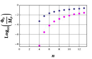
Figure 1: Estimates of the width (lower curve) and absolute upper bound (upper curve) for the distribution of flat direction VEVs as a function of the lowest nonzero term in the superpotential indexed by $n$ (see (38) and (116)). The width and upper bound curves are obtained from formulas (117) and (118). In the above $m\sim 10^{-16}M_{P}\sim TeV$ and $H\sim 10^{-6}M_{P}$ which is fixed by the COBE normalization for a quadratic inflaton potential (See Section 15)

Note that to keep the discussion in the previous section as simple as possible, the calculations were performed assuming a real scalar field. The MSSM flat directions however are complex scalars. The above results (117) and (118) are still valid for a complex field. However a complex scalars may also be charged under some symmetry. In the case of the MSSM flat directions, this charge is typically the difference in the baryon and lepton numbers, $B-L$ and the symmetry is the conservation of the $B-L$ charge. Our estimates of the variance would apply to the modulus of the complex field. One expects the phase of the field to be randomized as well, though the distribution need not be uniform on the circle if $C$ and/or $CP$ symmetries are explicitly violated in the theory.

Another consideration is that there are many MSSM flat directions, and if some set of them obtains large VEVs during inflation, then this may exclude another complementary set of flat directions from obtaining VEVs as a consequence of the large induced mass. Thus, when the quantum fluctuations of the flat directions are generated during inflation, there will be competition between mutually exclusive flat directions. If inflation lasts long enough, some set of the flat directions may have obtained large VEVs at the exclusion of a complementary set. As the process is random, some patches of the universe may be dominated by one set of VEVs and another patch may be dominated by a complementary set, and these may smoothly interpolate with patches with small or no VEVs at all. A comprehensive analysis of the resulting distributions of VEVs would be a difficult task, and far beyond the scope of this work. However for our purposes, it is sufficient for us to have made an estimate for the approximate width of these distributions as quantified in Figure 1.

What is relevant to our models is not the distribution of VEVs at the conclusion of inflation, but the distribution at a later time when $H\raisebox{-0.43057pt}{ $\begin{array}[]{@{}c}\scriptstyle<\\ \scriptstyle\sim\end{array}$}m$, and in particular the distribution’s tail. Our models will describe the evolution just after $R_{H\sim m}$. The motion from the end of inflation to this instant may in fact alter the shape of the distribution’s tail. These issues are discussed next.

14 Post-Inflation Classical Evolution of Flat Direction and Inflaton VEVs

In the previous two sections, the focus was on the statistical distribution of VEVs obtained by a flat direction by the conclusion of inflation. In particular, both a width and absolute upper bound to the distribution was estimated in (117) and (118) and shown in Figure 1. Because this thesis is focused on the fate of very large flat direction VEVs, we will consider only the range of initial VEVs from this distribution falling between these two bounds and we study their subsequent classical evolution after inflation has ended. In general, the distribution of VEVs valid at the end of inflation will be transformed to a slightly different distribution at the instant when $H\sim m$. After this instant, the classical evolution has a relatively simple form. This state of the evolution is also the stage relevant to our models. We then discuss the early generation and subsequent conservation of the $B-L$ charge belonging to the flat direction fields. Discussion of the quantum effects (decay) on the inflaton and flat directions after inflation is postponed to Section The Evolution and Decay of Supersymmetric Flat Directions in the Early Universe and Their Role in Thermalizing the Universe which builds upon the description here. Elements of the following discussion can also be found in [20, 33, 32, 74].

Recall from Section The Evolution and Decay of Supersymmetric Flat Directions in the Early Universe and Their Role in Thermalizing the Universe that inflation ends when the inflaton has evolved to a location on its potential when the slow-roll conditions (101) are no longer valid. Thus, the inflaton field begins to move in the sense ${\dot{\chi}}^{2}\sim V(\chi)$, and begins oscillations according to the equation of motion (93) and the Friedmann equation. The spatial gradient term is negligible compared to the other terms initially, so the inflaton remains a homogeneous field over the horizon volume as its oscillations begin. The solutions are damped oscillations (see Appendix The Evolution and Decay of Supersymmetric Flat Directions in the Early Universe and Their Role in Thermalizing the Universe) about $\chi=0$ with frequency $m_{\chi}\sim 10^{-6}M_{P}$,

$$\chi(t)=\frac{M_{p}}{\sqrt{3\pi}m_{\chi}t}\sin(m_{\chi}t)+{\cal O}\left(\frac{M_{P}}{(m_{\chi}t)^{2}}\right)$$ (121)

From this, one calculates the energy density of the inflaton in terms of the scale factor $R$ and one sees the evolution to be that of a matter dominated universe,

$$\rho_{\chi}\approx m_{\chi}^{2}M_{p}^{2}\left(\frac{R_{0}}{R}\right)^{3}$$ (122)

where $R_{0}$ is the scale factor at the onset of inflaton oscillations or equivalently, the end of slow roll inflation, and where the prefactor has been dropped in order to simplify later calculations. The behavior of the energy density as a function of the scale factor $\frac{R}{R_{0}}$ is shown in Figure 14.

Evolution of the energy density of the inflaton (solid curve) and a flat direction VEV (long dashes) at the conclusion of inflation. The horizontal axis is Logarithmic in the scale factor where $R_{0}$ is the scale factor at the onset of inflaton oscillations. The flat direction (long dashes) has been given an initial amplitude $|\Phi_{0}|\sim 10^{-2}M_{P}$ which corresponds to the the lower bound of Figure 1 with $n=10$. Also shown is a case assuming the same potential but with the VEV having reached the upper bound of Figure 1. In this latter case, the early motion of the flat direction (short dashed curve) is dominated by the higher order terms $V_{n>3}$ in the potential (116), and so the initial energy density can be orders of magnitude higher. However, assuming the field is in slow-roll, one may argue that $\rho_{\Phi}$ should decrease slightly faster than $\rho_{\chi}$ as shown for example in the short dashed curve. As $\Phi$ decreases, the terms $V_{n>3}$ in the potential (116) become comparable to the mass term, and the evolution is expected to smoothly transition between the two dashed curves (transition not shown). Note the analysis of this last case is somewhat heuristic and not by any means definite. Also shown are $R_{d\chi}$, the scale factor at the instant of the inflaton’s gravitational decay and $R_{eq}$, the scale factor at the instant the flat direction would overtake the inflaton (262) assuming $\Phi$ has not already decayed. For a comparable analysis on which this figure is based see [33]

Note, the inflaton energy density $\rho_{\chi}$ will dominate over the energy density of the flat direction initially and thus drive the Hubble parameter. The precise evolution of the flat direction is determined through the flat direction’s equations of motion and the Friedmann equation which are,

$$\ddot{\Phi}+3H\dot{\Phi}+\frac{dV}{d\Phi}=0$$ (123)

$$\left(\frac{\dot{R}}{R}\right)^{2}=\frac{8\pi G}{3}\left(|\dot{\Phi}|^{2}+V(\Phi)+\rho_{\chi}\right)$$

where we have assumed one complex degree of freedom for the flat direction $\Phi$, and where $V(\Phi)$ has the proposed form (116). To develop an understanding for how the flat direction evolves, consider two different scenarios for $\Phi_{0}$ which lie on the two curves of Figure 14. The scenario with $\Phi_{0}$ on the lower curve is simpler, so we begin with this. Recall from the previous section that in this scenario the mass term is comparable to the contribution of the higher order terms of the potential, $m^{2}\Phi^{2}\sim V_{n>3}$. At the conclusion of inflation, the field will be frozen, but will begin to move when the condition $\frac{d^{2}V}{d\Phi^{2}}\sim H^{2}$ is satisfied which is then the condition $m\sim H$. Thus the flat direction VEV is frozen until the scale factor $R_{m}$ as shown in Figure 14. Another way to state this is that the field value is nearly frozen until the age of the universe $H^{-1}$ is comparable to the period of one oscillation of the field $m^{-1}$. The inflaton will still be executing damped oscillations (121) at this instant. The subsequent motion of $\Phi$ will be discussed shortly.

Next consider the scenario with $\Phi_{0}$ on the larger bound (118) and thus on the higher curve of Figure 1. The energy density of the flat direction in this scenario can be many orders of magnitude above the first scenario, but still sub-dominant to the inflaton energy density (see Figure 14). Also in this scenario, the VEV will begin to move immediately at the conclusion of inflation, since $\frac{d^{2}V}{d\Phi^{2}}\sim H^{2}$ is satisfied immediately. The exact motion of $\Phi$ at the onset of inflaton oscillations depends on the nonlinearities of the potential. When the field moves, it is reasonable to assume that the energy density will decrease as fast or faster than the inflaton. For instance, if one assumes the field is in slow-roll (neglecting $\ddot{\Phi}$ in the equation of motion), then this may be shown. A situation such as this is depicted in Figure 14. In this case, the energy density would decrease as fast or fast than the inflaton until the mass term becomes comparable to the higher order terms of the potential $m^{2}|\Phi|^{2}\sim V_{n>3}(\Phi)$. At this instant, the field would reside on the lower curve of Figure 1. The evolution would then smoothly make a transition to the case of a mass dominated potential which was described above. During this whole phase of the evolution the assumption is that the field is in slow roll. What we draw from this analysis is that initial field values larger than the width (117) may evolve to approximately the same field value and energy density at the instant $H\sim m$.

After this instant $H\sim m$, the equation of motion (123) is approximately linear in $\Phi$, and the motion will be that of damped linear oscillator with a time dependent damping term $H$. The solutions are similar to that of the inflaton,

$$\Phi\approx\left(\frac{R_{m}}{R}\right)^{3/2}\Phi_{m}\left[A_{r}\cos(mt+\delta_{r})+iA_{i}\sin(mt+\delta_{i})\right]+{\cal O}\left(\frac{R_{m}^{3}}{R^{3}}\right)$$ (124)

which evolves with a matter-like energy density,

$$\rho_{\phi}\sim m_{\phi}^{2}\Phi_{m}^{2}\left(\frac{R_{m}}{R}\right)^{3}$$ (125)

and with $A_{r}$, $A_{i}$, $\delta_{r}$, $\delta_{i}$ being dimensionless coefficients of the evolution. Three of these coefficients are fixed by initial conditions and the fourth is fixed by the normalization,

$$A_{r}^{2}\cos^{2}\delta_{r}+A_{i}^{2}\sin^{2}\delta_{i}=1$$ (126)

This evolution is shown for a sample set of parameters in Figure 2 where one sees the field executes a elliptic-like trajectory about the origin while spiralling to smaller values due to Hubble expansion.

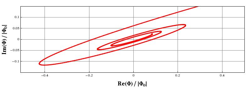
Figure 2: Evolution of the complex scalar field $\Phi$ for a sample choice of parameters. The parameters chosen are $A_{i}=\frac{1}{2}$, $A_{r}=-\sqrt{\frac{15}{8}+\frac{17}{8\sqrt{5}}}$, $\delta_{i}=\frac{\pi}{10}$, and $\delta_{r}=\frac{7\pi}{10}$. The charge asymmetry as computed by formula (128) is $\epsilon_{B-L}=\frac{1}{8}\sqrt{7-\frac{6}{\sqrt{5}}}\approx 0.26$

During this time of damped linear oscillations, the ratio of the flat directions energy density to that of the inflaton is fixed to the following ratio (assuming the inflaton and/or flat direction have not already decayed),

$$\frac{\rho_{\Phi}}{\rho_{\chi}}\sim\left(\frac{\Phi_{m}}{M_{P}}\right)^{2}$$ (127)

and we see that so long as $\Phi_{m}<M_{p}$, the inflaton will dominate the total energy density. If this condition is not satisfied, then the flat direction will overtake the inflaton even before the flat direction begins oscillations. As we have just discussed, the higher order terms in the potential, if present, will keep the flat direction VEV bounded below the Planck mass.

One other element to the classical evolution of the flat direction is the charge associated with the motion of the flat direction. The charge of the flat direction is not a standard model gauge charge but rather it will typically be the difference of lepton number and baryon number $B-L$. The field $\Phi$ is then by definition a gauge singlet field. As was mentioned in the previous subsection 13, the phase of the flat direction VEV is also randomized during inflation, though the distribution would presumably depend on the specific breaking of $C$ and $CP$ symmetries of ones model. Additionally if there exist $B-L$ violating interactions such as those discussed in Section 5 which involve the flat direction fields, then a $B-L$ charge can be generated dynamically through the flat directions classical equations of motion. This is essentially the well known baryogenesis mechanism of Affleck and Dine [20]. If inflation has driven the flat direction VEVs close enough the lower curve of Figure 1, then such nonlinear terms if present can in principle contribute a phenomenologically relevant $B-L$ charge. Once the field has reduced in amplitude past $H\sim m$, the charge will then be conserved. The charge in this regime is determined from our solutions (124) as follows,

$$n_{B-L} = (i\Phi^{*}\dot{\Phi}-i\dot{\Phi}^{*}\Phi)$$

$$= -\left(\frac{R_{m}}{R}\right)^{3}(m\Phi_{m}^{2})A_{i}A_{r}\cos(\delta_{i}-\delta_{r})$$

and the number charge per co-moving volume $(n_{B-L}R^{3})$ is thus conserved. Notice, the charge can take positive and negative values which will correspond to the handedness of the rotation of its trajectory in the complex plane. Also notice that given the constraint (126), the charge density is extremized when $(\delta_{i}-\delta_{r})=\pm\pi$ and $A_{i}=A_{r}=1$, and in the case $\delta_{i}-\delta_{r}=\pm\pi/2$, the charge is zero. Defining the ratio of the $B-L$ number charge density to the total particle density as the parameter $\epsilon_{B-L}$, one determines,

$$\epsilon_{B-L}\equiv\left|\frac{n_{B-L}}{n_{\Phi}}\right|=A_{i}A_{r}\cos(\delta_{i}-\delta_{r})$$ (128)

where this ratio was determined at $R_{m}$. The quantity $\epsilon_{B-L}$ is the $B-L$ number per particle of the condensate, and it is bounded between $\pm 1$. In the absence of $B-L$ violation, the net charge should be zero and the ellipse will have collapsed to a line passing through the origin. In the above we have parametrized the motion, but we have not explained how the charge asymmetry is developed through the nonlinear terms. An example of such terms was introduced in 40. To see how a charge is developed, redefine $\Phi$ such that its initial phase is zero and thus $\Phi$ initially lies on the real axis. As discussed after (40) this field redefinition implies $\lambda$ is explicitly complex (not on the real axis). Also assuming $\dot{\Phi}=0$ initially, the equation of motion for the imaginary part of $\Phi$ at the initial time reduces to

$$\ddot{\Phi}_{\rm{Im}}=-\mbox{Im}[\lambda]\Phi_{\rm{Re}}^{3}$$ (129)

and thus the field will begin to rotate off the real axis into the complex plane. Whether the rotation is clockwise or counter-clockwise depends on the phase of $\lambda$. In our later numerical simulations we will instead take $\lambda$ to be Real valued and the initial phase to be nonzero which is an equivalent situation. The amount of baryon asymmetry (computed later in Section 17) is dependent largely on the initial VEV $\Phi_{0}$ as well as on the existence of interactions such as (40). At later times when the higher order interactions such as these become sub-dominant to the mass term, the built up charge will be conserved to a good approximation [20]. The $B-L$ asymmetry may also be smaller or larger depending on how the inflaton and flat directions proceed to evolve. For instance if the flat direction energy density can overtake that of the inflaton, the baryon asymmetry can be order one. This situation would require very large sources of later entropy to dilute the $B-L$ charge density to be phenomenologically viable. Alternatively, if the inflaton remains the dominant fluid, the $B-L$ asymmetry obtains a suppression inversely proportional the amount of entropy released by inflaton decay. These issues will be discussed again in Section The Evolution and Decay of Supersymmetric Flat Directions in the Early Universe and Their Role in Thermalizing the Universe.

15 COBE Normalization and the Energy Scale of Inflation

Before continuing with our discussion of the evolution of the flat direction fields, we make a brief digression to discuss two very important inputs to our study from observational cosmology. These are phenomenological constraints on the Hubble parameter during inflation, $H_{I}$ obtained from the Cosmic Microwave background observations. As we have seen from the previous section in the results (107-115) the Hubble parameter or equivalently the energy scale of inflation controls the amplitude of the perturbations one obtains for a light scalar test field present during inflation. It can be shown that the amplitudes of the perturbations of the scalar and tensor modes of the gravitational field (primordial density perturbations and gravity waves) are also controlled by the Hubble parameter in a similar way [17, 75]. A large value for $H_{I}$ thus implies large cosmological perturbations which may be in conflict with observations of the CMB. The cosmological perturbations are not the focus of this thesis, but we shall briefly describe a constraint on $H_{I}$ related to the tensor modes as well as a constraint between $H_{I}$ and inflaton’s potential known as the COBE normalization, related to the scalar modes.

The tensor modes are like the scalar test fields just discussed in that the only physical parameter which appears in their spectrum is the Hubble Parameter [17, 75]. In this sense, a signature of primordial gravitational waves in the CMB is a direct measure of the energy scale of inflation. If one supposes the gravitational waves are a sizeable contribution to the CMB anisotropy, then the measured anisotropy places an upper bound on $H_{I}$ which is approximately,

$$H_{I}\lesssim 10^{-4}M_{P}$$ (130)

where $H_{I}$ is the Hubble parameter at the end of inflation. This bound is very conservative as the primordial gravitational wave contribution to the CMB is expected to be sub-dominant.

The scalar modes of the gravitational field are proportional to the perturbations of the inflaton field via Einsteins equation. The scalar modes may also be written in terms of the density perturbations $\frac{\delta\rho}{\rho}$ at the time of last scattering of the CMB photons, and these are related to the measured angular anisotropies of the CMB. Without going into these details, one obtains the COBE normalization of the inflaton’s potential which is,

$$\frac{H_{I}^{2}}{10\pi^{3/2}\dot{\chi}} \sim \frac{\delta\rho}{\rho}$$ (131)

$$\frac{V^{3/2}}{M_{P}^{3}V^{\prime}} \sim 10^{-5}$$ (132)

where the slow-roll approximation has been applied and where $H_{I}$ and $\chi$ are taken at the instant of 60 e-folds from the end of inflation which are to match the amplitude of the density perturbation on the largest observable scales today. The left-hand-side of this expression is proportional to the spectrum of perturbations, which again scales with powers of $H_{I}$, but the spectrum is also dependent on the shape of the potential which appears in the denominator of the second expression as $V^{\prime}$. The COBE normalization (132) is a “normalization” of $V(\chi)$ because, once the shape of the potential has been specified, then this equation fixes the value of $H_{I}$ or equivalently fixes the energy scale. For example, the inflaton potential we consider is a quadratic potential $V(\chi)=\frac{1}{2}m_{\chi}^{2}\chi^{2}$. Using the above formula, one obtains,

$$m_{\chi}\sim 10^{-6}M_{P}$$ (133)

which is the value we will apply throughout. From this one determines the Hubble parameter at the end of inflation to be $H_{I}\sim 10^{-6}M_{P}$.

The implications of the COBE normalization cannot be underestimated (For a general discussion, see [5]). Once one chooses a form for the inflaton potential, the COBE normalization, sets the energy scale for all of the field dynamics and particle decays which follow inflation. In setting the energy scale it also suggests the particle theories which one may choose to study. For example, the quadratic inflaton potential considered is the simplest one can imagine in the chaotic inflation paradigm. This falls into the class of polynomial potentials of which many models of inflation can be mapped into [64, 7]. The COBE normalization then yields approximately the same energy scale $H_{I}\sim 10^{16}\;GeV$ for all these potentials [7] which is also the energy scale $M_{GUT}$, at which the three gauge couplings appear to unify (see Figure 3). It is thus natural to consider supersymmetry and Grand Unified theories in combination with these potentials because one can then make predictions for the dynamics of these theories.

It is worth noting that the quadratic potential is consistent with CMB observations, though other potentials such as a quartic potential are now disfavored [19]. We note finally that some models of inflation can allow for a lower energy scale of inflation. Many of these are well motivated and consistent with observations, but do not easily fit into the context of our discussion which assumes supersymmetry, $B-L$ violating effects from the GUT scale, and large vacuum expectation values of flat direction fields which are generic to supersymmetric theories, but may not be present in other theories. We return to the discussion of the dynamics and decay of the inflaton and flat direction fields.

Chapter Reheating and Preheating

In this section we describe reheating, which is the process by which the large entropy of the universe is generated through the decay of the inflaton and through the subsequent thermalization of the inflaton decay products. Reheating is thus the particle genesis for the universe. A target quantity in the study of reheating is the reheat temperature $T_{RH}$ which is the temperature of the inflaton’s decay products once they have thermalized (assuming the inflaton energy density dominates). Another target quantity is the baryon asymmetry quantified by the difference of the baryon and lepton number densities divided by the entropy density, $\frac{n_{B-L}}{s}$. This quantity is expected to be conserved after the universe has reached a thermal state, and is related to the observed baryon to photon ratio today [76]. There are other possible observables related to reheating which will be mentioned at the conclusion of this section, but the focus here will be on $T_{RH}$ and $\eta_{B}$ both of which are dependent upon the dynamics of the flat directions.

To begin, a framework for determining $T_{RH}$ and $\eta_{B}$ is outlined, based on the Hubble parameter during inflation, $H_{I}$ the decay rate of the inflaton $\Gamma_{\chi}$, and the rate of thermalization of the inflaton decay products $\Gamma_{therm}$. We then discuss three perturbative decay scenarios of the inflaton; decay into fermions, decay into scalars, and a Planck suppressed decay. We describe the subsequent thermalization process of the inflaton decay products in the absence of flat direction VEVs, and then in their presence, explaining how in the latter case the thermalization may be delayed due to the effective vacuum established by the flat directions. However, this presumes the flat directions persist in a coherent state for a relatively long time. We note that the perturbative decay channels of the flat direction are suppressed by powers of the VEV [20], so this presumption is not unwarranted, but indications are that a fast nonperturbative decay of the flat direction VEV may be possible [26]. To motivate the analysis of nonperturbative flat direction decay, we discuss the now well studied nonperturbative decay of the inflaton commonly referred to in the literature as “preheating” [56]. Based on this analysis we present a preliminary discussion of the nonperturbative decay of the flat directions. Figure The Evolution and Decay of Supersymmetric Flat Directions in the Early Universe and Their Role in Thermalizing the Universe shows how the elements in the above scenarios are related. The reader is also referred to the following books and reviews from which the background material here was gathered [5, 16, 67, 63, 64, 70].

Schematic of the model of reheating involving flat directions. For the inflaton, decay may proceed via couplings to fermions and/or bosons through perturbative or nonperturbative mechanisms. The inflaton may also decay through gravitationally suppressed coupling (perturbative decay). Also shown is the flat direction evolution. The flat directions establish an effective vacuum into which the inflaton will decay and in which its products will thermalize, but the vacuum is effective only as long as the flat direction VEV remains coherent. Thermalizing interactions can be suppressed due to exchanged particles having very large effective masses. Additionally, the flat direction VEVs perturbative decay rate is strongly suppressed (see equation (157)) for the same reason that the mediating particles are very massive [20]. If the VEV is sufficiently long lived, its energy density may come to dominate over that of the inflaton. If this happens, the reheating temperature $T_{RH}$ will be determined by flat direction decay and thermalization of its decay products instead of that of the inflaton. The figure shows the case of inflaton domination because our belief is that flat directions will decay quickly by nonperturbative mechanisms and thus removing its induced effective vacuum. Such nonperturbative decay mechanisms are introduced in this section and further developed in the remaining sections.

16 Determining the Reheating Temperature

Here we continue to develop the picture of the post-inflation evolution of the inflaton and flat directions which was begun in Section 14. The emphasis in the previous discussion was on the classical evolution of these fields. The emphasis here is on quantum effects, namely the decay rates of these fields $\Gamma_{\chi}$, and $\Gamma_{\Phi}$, as well as the rate of thermalization of the inflaton decay products, $\Gamma_{therm}$. While the basic picture is developed, a simple framework for calculating the reheating temperature $T_{RH}$ and the baryon asymmetry is also established. The main difficulty and the main source of uncertainty is the reliable computation of the decay rates and thermalization rates and this is postponed to the next section.

To begin, consider the following simple upper bound for the reheat temperature which assumes that at the end of inflation, the inflaton decays in less than one Hubble time. Specifically, all of the inflaton condensate decays and thermalizes with negligible decrease in the total energy density in less than one Hubble time. Under these assumptions, and applying the upper bound on the Hubble parameter during inflation, $H_{I}<10^{-4}M_{p}$ discussed in Section 15, we equate $H_{I}$, to the Hubble parameter during a thermal radiation dominated epoch during which time the temperature is related to $H$ as follows (see (260)),

$$T=\left(\frac{45}{4g_{*}\pi^{3}}\right)^{1/4}\sqrt{HM_{P}}\hskip 40.00006ptg_{*}(T)=g_{b}+\frac{7}{8}g_{f}$$ (134)

where $g_{*}(T)$ is the effective number of relativistic (massless) degrees of freedom at the temperature $T$ with $g_{b}$ and $g_{f}$ being the number of bosonic and fermionic degrees of freedom. In the standard model $g_{*}=106.75$, and for supersymmetric GUTs $g_{*}\raisebox{-0.43057pt}{ $\begin{array}[]{@{}c}\scriptstyle<\\ \scriptstyle\sim\end{array}$}1000$ from which we may obtain a convenient formula for the reheating temperature

$$T_{RH}\sim 0.1\sqrt{H_{RH}M_{P}}$$ (135)

where $H_{RH}$ is the Hubble parameter at the instant of thermalization. From this expression and the upper bound $H_{I}<10^{-4}M_{P}$, one determines,

$$T_{RH}<10^{16}\;GeV$$ (136)

which is thus an absolute upper bound on $T_{RH}$ independent of any assumptions on the inflaton’s potential or other interactions. An absolute lower bound on the reheating temperature is obtained from the fact that nucleosynthesis occurs in a thermal bath at a temperature of approximately 1 MeV [77], so

$$T_{RH}\gtrsim 10^{-3}GeV$$ (137)

It is remarkable that there exists approximately $19$ orders of magnitude of uncertainty in $T_{RH}$. However, the above are phenomenological bounds on $T_{RH}$. If one makes assumptions on the particle theory applicable during reheating, this range may be narrowed. We will make some minimal assumptions on our particle theory in order to estimate the reheating temperature, the first of which is an assumption of a quadratic inflaton potential $\frac{1}{2}m_{\chi}^{2}\chi^{2}$ whose mass $m_{\chi}\sim 10^{-6}M_{P}$ is fixed by the COBE normalization (133). This assumption also fixes the Hubble Parameter at the end of inflation,

$$H_{I}\sim 10^{-6}M_{p}\hskip 20.00003pt\mbox{with}\hskip 20.00003ptV(\chi)=\frac{1}{2}m_{\chi}^{2}\chi^{2}$$ (138)

so if the inflaton were to decay and thermalize instantly (within one Hubble time) the reheating temperature in this case is $\sim 10^{15}\;GeV$ which is six orders of magnitude above the temperature on needs to avoid an overproduction of the gravitinos   In light of this, one may look for mechanisms which would suppress either the inflaton’s decay or the thermalization of its products. In particular, the role of flat directions in suppressing the thermalization of the inflaton decay products will be discussed in the following subsections. However, before making such assumptions, we erect a simple framework for determining $T_{RH}$ as well as the baryon asymmetry $\eta_{B}$ with model assumptions entering through decay and reaction rates $\Gamma_{i}$. The only further assumptions we make in this framework are the quadratic inflaton potential, and the Friedmann equation.

We determined in Section 14 the classical evolution of both the inflaton and a flat direction after the inflationary stage. The solutions are damped oscillations of the form (121) for the inflaton with frequency $m_{\chi}\sim 10^{-6}M_{P}$ and (124) for a flat direction with frequency $m\sim 10^{-16}M_{P}$. For both of these homogeneous scalar fields, there is an equivalent quantum interpretation as zero temperature (and thus zero momentum) condensates of scalar particles of mass $m_{\chi}$ and $m$ respectively. These particles can have decay mechanism(s) into lighter species which we parametrize with the decay rates $\Gamma_{\chi}$ and $\Gamma_{\phi}$. The decays are quantum effects which modify the respective classical equations of motion. Consider for instance, the inflaton. One estimates the number of $\chi$ particles in the inflaton condensate as,

$$n_{\chi} = \frac{\rho_{\chi}}{m_{\chi}}=\frac{1}{2m_{\chi}}\left({\dot{\chi}}^{2}+m_{\chi}^{2}\chi^{2}\right)$$ (139)

$$\approx \frac{\dot{\chi}^{2}}{m_{\chi}}\approx m_{\chi}\chi^{2}$$ (140)

where the virial theorem has been applied in the last two steps to approximate the number density. The reaction rate equation for the $\chi$ particles is

$$\frac{1}{R^{3}}\frac{d(R^{3}n_{\chi})}{dt}=-\Gamma_{\chi}n_{\chi}\\$$ (141)

where $n_{\chi}$ is the number density of the inflaton condensate. Substituting the expressions for the number density $n_{\chi}$, we obtain,

$$\ddot{\chi}+(3H+\Gamma_{\chi})\dot{\chi}+m_{\chi}^{2}\chi = 0$$ (142)

which is the equation of motion (93) including a decay term which appears on the same footing as the Hubble parameter.  A similar equation may be derived for the complex flat direction field. For the moment, we consider just the inflaton decay based on the equation (142). When the decay rate is small compared to the Hubble parameter $\Gamma_{\chi}<H$, the solution to the equations of motion is the result (121). Though when the expansion has slowed to a point where $H\raisebox{-0.43057pt}{ $\begin{array}[]{@{}c}\scriptstyle<\\ \scriptstyle\sim\end{array}$}\Gamma_{\chi}$, the decays soon dominate over the coherent classical oscillation, and the condensate is soon depleted. This happens at a value of the scale factor we define as $R_{d\chi}$. Since the inflaton mass is orders of magnitude above the mass of most of its expected decay products, the products will be relativistic. For $R>R_{d\chi}$, that is after inflaton decay, the energy density evolves in a radiation dominated universe (see Figure 14). In this regime after the initial decay, the decay products are not necessarily in a thermal state however [33], and there will be scatterings, particle creation and particle destruction to bring the system to a thermal and chemical equilibrium [33, 85]. This thermalization rate is parametrized with a second reaction rate $\Gamma_{therm}$. If, at the time of decay, the thermalization rate is faster than the Hubble expansion, which implies $\Gamma_{therm}>\Gamma_{\chi}$, then thermalization can be thought of as happening instantly at $R_{d\chi}$. The reheat temperature is then determined with (135) by setting $H\sim\Gamma_{\chi}$ in this expression. If on the other hand the thermalization process is slow, and $\Gamma_{therm}<\Gamma_{\chi}$, then the reheating temperature is determined by setting $H\sim\Gamma_{therm}$ in this expression. Summarizing,

$$T_{RH}\sim 0.1\sqrt{H_{RH}M_{P}}\;\;\;,\;\;\;H_{RH}\sim\mbox{Min}[\Gamma_{\chi},\Gamma_{therm}]$$ (143)

Reheating is thus determined by the slowest reaction rate. Note that we nowhere assumed the reaction rates $\Gamma_{\chi}$ and $\Gamma_{therm}$ were perturbative results. The rate $\Gamma_{\chi}$ in particular can equivalently parametrize a nonperturbative decay.

The presence of flat directions with large vacuum expectation values can modify the above history of reheating through the value of inputs $\Gamma_{\chi}$ and $\Gamma_{therm}$. Furthermore, if the flat directions have large enough expectation values, and if they are sufficiently long lived, the flat directions can come to dominate the total energy density. For this to happen, the inflaton must decay before or during the flat directions oscillations so that the ratio $\rho_{\Phi}/\rho_{\chi}$ is no longer constant but scales as $R$ until a significant portion of the flat direction particles decay or up-scatter into a relativistic species (see Section 14 and Figure 14). Referring to figure 14, the value of the scale factor at which the flat direction energy density would overtake that of the inflaton is obtained in (262) to be

$$\frac{R_{eq}}{R_{0}}\sim\left(\frac{M_{P}}{\Phi_{0}}\right)^{2}\left(\frac{m_{\chi}}{\Gamma_{\chi}}\right)^{2/3}$$ (144)

Then assuming that the flat direction decay rate $\Gamma_{\Phi}$ is a constant, the condition for the flat direction to dominate is that $R_{eq}<R_{d\Phi}$ which may be rewritten (see formula (263)),

$$\frac{\Gamma_{\Phi}}{\Gamma_{\chi}}<\left(\frac{\Phi_{0}}{M_{P}}\right)^{4}$$ (145)

The region of flat direction domination is shown in the plane $(\Phi_{0},\Gamma_{\Phi})$ in Figure 20.

One may also wish to compute the reheating temperature in these cases when the flat direction dominates, but they imply a baryon asymmetry of order one, and thus require either an extremely small $\epsilon_{B-L}$ or a later “additional” source of entropy to dilute the B-L charge to the required amount. As the first case is not obviously natural and the second case adds complications to the simple picture of inflation, flat direction domination is not pursued here any further than establishing the parameter boundaries in Figure 20.

17 Determining the Baryon Asymmetry

The next task is to estimate the baryon asymmetry within the above context. It was noted in Section 4 that the MSSM flat directions may carry a $B-L$ charge. It was also mentioned that such a charge may be generated by the early motion of the flat direction through Planck suppressed $B-L$ violating interactions, and afterwards approximately conserved. While only a baryonic charge is strictly necessary for baryogenesis, it may be that a nonzero $B-L$ charge is required [79], though see [80]. The reason is that the sum of the baryon and lepton numbers $B+L$ is violated by Electroweak processes known as sphalerons. Howver the quantity $B-L$ is conserved by Electroweak interactions, so any baryon asymmetry generated may be erased by these sphaleron processes when they are in equilibrium [79].

In the following we will estimate the quantity $\frac{n_{B-L}}{s}$ which is the ratio of the $B-L$ number density to the entropy density. This quantity is an adiabatic invariant since the $B-L$ number per co-moving volume $R^{3}n_{B-L}$ is conserved soon after the flat direction oscillations begin and the entropy per co-moving volume $R^{3}s$ is conserved from $T_{RH}$ to the present epoch. The conversion of $B-L$ to $B$ by sphalerons is quantified approximately by the relation [81],

$$n_{B}=\frac{28}{79}n_{B-L}$$ (146)

The baryon-to-entropy ratio today is $\left(\frac{n_{B}}{s}\right)_{obs}\sim 10^{-10}$ which is obtained from the observed baryon-to-photon ratio. A challenge for any fundamental particle theory is to obtain this baryon-to-entropy ratio from first principles. There are many proposed mechanisms of baryogenesis [82], but the mechanism which is intimately connected with the study of flat directions is that of Affleck and Dine [20]. We next compute the baryon to entropy ratio in the Affleck Dine baryogenesis scenario.

Recall from Section 14, the number density $n_{B-L}$ is computed from the classical trajectory (128), and once generated the $B-L$ number per co-moving volume is then nearly conserved. The resulting baryon to entropy ratio depends on how much this charge is diluted by the entropy generated through inflaton decay and thermalization. Specifically, the entropy per co-moving volume is not fixed until after a thermal state is reached at $T_{RH}$, so it should be computed at or after this instant. However, the resulting expression is the same if it were computed at the time of inflaton decay. The reason is that we have assumed the inflaton energy density dominates throughout, and the inflaton decay products behave like radiation before and after thermalization. The entropy density is related to the energy density through $s\sim\rho_{rad}^{3/4}$ from (261), so the entropy per co-moving volume is largely insensitive to when the inflaton decay products thermalize. The main approximation here is that the flat direction energy density is negligible compared to the inflaton energy density. As shown in Figure 14, the dominance of the inflaton is not guaranteed. The entropy density and the $B-L$ number density are both computed at the time of inflaton decay $R_{d\chi}$ to obtain the desired ratio,

$$\frac{(n_{B-L}R^{3})_{d\chi}}{(sR^{3})_{d\chi}} \sim \left(\frac{\epsilon_{B-L}\frac{\rho_{\Phi}}{m}}{\rho^{3/4}}\right)_{d\chi}$$ (147)

$$\sim \epsilon_{B-L}\left(\frac{\rho_{\Phi}}{\rho_{\chi}}\right)_{d\chi}\frac{\rho_{d\chi}^{1/4}}{m}$$ (148)

$$\sim \epsilon_{B-L}\left(\frac{|\Phi_{0}|}{M_{P}}\right)^{2}\left(\frac{\Gamma_{\chi}}{M_{P}}\right)^{1/2}\left(\frac{M_{P}}{m}\right)$$ (149)

where in the last step, the relation (127) has been applied as well as the relation $\rho_{d\chi}\sim\Gamma_{\chi}^{2}M_{P}^{2}$ which follows from $H_{d\chi}\sim\Gamma_{\chi}$ and the Friedmann equation. The baryon-to-entropy ratio is then estimated using the sphaleron conversion (146) and assuming a gravitational decay $\Gamma_{\chi}\sim\frac{m_{\chi}^{3}}{M_{P}^{2}}$ with $m_{\chi}\sim 10^{-6}M_{P}$, $m\sim 10^{-16}M_{P}$. One obtains,

$$\frac{n_{B}}{s}\sim\epsilon_{B-L}\left(\frac{\Phi_{0}}{M_{P}}\right)^{2}10^{7}$$ (150)

Recall from (128) that $\epsilon_{B-L}$ quantifies the $B-L$ number per particle in the flat direction condensate with $\epsilon_{B-L}=\pm 1$ corresponding to a maximally charged condensate. Also, our constraint that the inflaton energy density dominates translates to the constraint $\Phi_{0}<M_{P}$ as shown in (127). Using both considerations, the above baryon to entropy ratio may still be significantly greater than one if the condensate is maximally charged and $\Phi_{0}\raisebox{-0.43057pt}{ $\begin{array}[]{@{}c}\scriptstyle<\\ \scriptstyle\sim\end{array}$}M_{p}$. It has been argued by Linde [21] that generically the baryon to entropy ratio should not exceed one. In the example given in [21], it is the thermal corrections to the masses of the states involved which result in the ratio being bounded below unity, but the example assumes a case of flat direction domination. It is not immediately obvious how one would generalize such arguments to our situation and assumptions. We do not attempt such corrections here. The above ratio (150) is sufficient to establish the leading dependence on the parameters $\Phi_{0}$ and $\epsilon_{B-L}$. Specifically, one concludes that to have a successful Affeck-Dine baryogenesis, one requires either $\epsilon_{B-L}\ll 1$ and/or $\Phi_{0}\ll M_{P}$ given our assumption of a gravitational decay (and precluding any additional contributions of entropy such as from moduli decay). We emphasize that the baryon asymmetry, while sourced by early motion of the flat direction, appears to be largely independent of the flat direction’s later dynamics, so long as the inflaton dominates the energy density. This result for the baryon to entropy ratio (150) and the above brief qualifications are thus the conclusion of our discussion of baryogenesis.

18 Perturbative Decay and Thermalization of the Inflaton

The perturbative decay of the inflaton and thermalization of its decay products was studied shortly after the first models of inflation were developed [83] (see also the text-books [16, 84]). In the following, we briefly present the generic scenarios as well as some recent developments regarding the thermalizing interactions which follow inflaton decay [85].

In the absence of a flat direction VEV, the inflaton decays into a vacuum in which supersymmetry is assumed to be softly broken at a scale $m_{\mathrm{susy}}\sim\mathrm{TeV}$. We assume that there exist light states $m_{\psi},m_{\xi}\ll m_{\chi}$ in this vacuum to which the inflaton can decay, specifically, spin 1/2 fermions via $\chi\rightarrow\psi\psi$ or spin-0 bosons via $\chi\rightarrow\xi\xi$. The corresponding terms in the Lagrangian would appear as,

$${\cal L}_{int}=-g\chi\xi^{2}-h\chi\bar{\psi}\psi$$ (151)

where the coupling $h$ is dimensionless, and $g$ has dimensions of mass. The decay rates for these interactions can be computed, and assuming that the final states have masses $m_{\psi},m_{\xi}\ll m_{\chi}$, the perturbative decay rates are,

$$\Gamma(\chi\rightarrow\xi\xi)=\frac{g^{2}}{8\pi m_{\chi}}\;\;\;,\;\;\;\Gamma(\chi\rightarrow\psi\psi)=\frac{h^{2}m_{\chi}}{8\pi}$$ (152)

The form of these rates could also be obtained from dimensional analysis. In the case these rates are gravitationally suppressed, one has $g\sim m_{\chi}\left(\frac{m_{\chi}}{M_{P}}\right)$ and $h\sim\frac{m_{\chi}}{M_{P}}$, resulting in,

$$\Gamma_{Grav}\sim\frac{m_{\chi}^{3}}{M_{p}^{2}}$$ (153)

which could also have been obtained by dimensional analysis and independently of the spin of the final state particles. The gravitationally suppressed decay would proceed in approximately $\frac{m_{\chi}}{2\pi\Gamma_{Grav}}\sim 10^{13}$ oscillations of the inflaton. To determine $T_{RH}$ assuming the gravitational decay, the thermalization rate $\Gamma_{\mathrm{therm}}$ must be computed. We use the results of [85] in which it is shown that a thermalization process can be expanded in a series involving the coupling $\ga$ as well as the small quantity $\frac{T_{RH}}{m_{\chi}}$ which quantifies how effective the process is at transferring the high momenta inflaton products $k\sim m_{\chi}$ to the reheat temperature. It is shown in [85] that the dominant thermalization processes after perturbative inflaton decay are $2\rightarrow 3$ inelastic scattering with a rate,

$$\Gamma_{2\rightarrow 3}\sim\ga\left(\frac{m_{\chi}}{T_{RH}}\right)^{2}\Gamma_{2\rightarrow 2}$$ (154)

$$\Gamma_{2\rightarrow 2}\sim n_{\chi}\sigma\;\;\;,\;\;\;\sigma=\left(\frac{\ga}{m_{\chi}}\right)^{2}\left(\frac{R}{R_{d\chi}}\right)^{2}$$ (155)

where $\Gamma_{2\rightarrow 2}$ is the elastic scattering rate, $\sigma$ is the corresponding elastic cross-section, and $n_{\chi}$ is the number density for the inflaton condensate (which should be of the same order as the number density of its decay products).

Note that the thermalization rate $\Gamma_{2\rightarrow 3}$ is suppressed by three powers of the gauge coupling $\ga^{3}$, but then enhanced by the factor $\left(\frac{m_{\chi}}{T_{RH}}\right)^{2}$ which quantifies the processes efficiency in momentum transfer. One may determine the the thermalization rate and reheat temperature by a self-consistent method by first assuming $\Gamma_{\mathrm{therm}}>\Gamma_{\chi}$ so that $T_{RH}\sim\sqrt{\Gamma_{\chi}M_{P}}$, and then determining the conditions on the parameters for this to be true. By this method, one requires the gauge coupling to satisfy $\ga^{-1}>100$ (see (272) and reference [26]). Keeping in mind that this is an order of magnitude approximation, this condition on $\ga$ may be compared against the expected values of the gauge couplings, shown in Figure 3, where one would presumably choose the renormalization scale at or near a momentum transfer of order $Q\sim T_{RH}$. Assuming the condition on the gauge couplings is satisfied, the thermalization happens immediately after inflaton decay and the reheat temperature is

$$T_{RH}\sim 10^{9}\;\mathrm{GeV}\hskip 30.00005pt\mbox{gravitational decay, w/o flat direction VEVs}$$ (156)

Again, this temperature corresponds to the gravitationally suppressed decay (153) in the absence of flat directions. It will be a reference case in the remaining discussion.

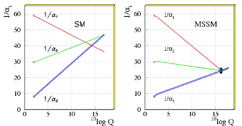
Figure 3: Running of the gauge couplings in the standard model and the MSSM. The inflaton decay products are expected to thermalize through gauge interactions. With our assumptions, one expects the typical momentum transfer of the interactions to be $T_{RH}\raisebox{-0.43057pt}{ $\begin{array}[]{@{}c}\scriptstyle<\\ \scriptstyle\sim\end{array}$}10^{9}\,\mathrm{GeV}$ from (156). Thus the relevant gauge couplings can be read from the righthand plot at $Q\sim 10^{9}\,\mathrm{GeV}$. Note also the apparent gauge coupling unification in the MSSM at the scale $M_{GUT}\sim 10^{16}\,\mathrm{GeV}$. Figure obtained from [76]

19 Perturbative Decay and Thermalization of the Inflaton With Flat Directions

Next we consider the effect of flat direction VEVs on the inflatons decay rate $\Gamma_{\chi}$ and on the thermalization rate of the decay products $\Gamma_{therm}$. During inflation, a subset of the MSSM flat directions have presumably accumulated a large condensate of particles in their zero momentum state (these are the VEVs). It is useful to think of this condensate as an effective vacuum. From Section The Evolution and Decay of Supersymmetric Flat Directions in the Early Universe and Their Role in Thermalizing the Universe, it was noted that this vacuum typically breaks all the standard model gauge symmetries, and thus the spectrum of particles is quite different than the unbroken vacuum. In particular, the induced particle masses are of order of the obtained VEVs which may be nearly at the Planck Mass. One notes however that the VEVs evolve slowly in time with frequencies $\sim m_{\mathrm{susy}}$ as discussed in Section 14. For the inflaton whose mass is much greater than $m_{\mathrm{susy}}$, the vacuum will look stationary. However, for the light states of mass $\raisebox{-0.43057pt}{ $\begin{array}[]{@{}c}\scriptstyle<\\ \scriptstyle\sim\end{array}$}m_{\mathrm{susy}}$ the vacuum will be moving relatively fast assuming the particle momenta is small, $k\raisebox{-0.43057pt}{ $\begin{array}[]{@{}c}\scriptstyle<\\ \scriptstyle\sim\end{array}$}m_{\mathrm{susy}}$. There can be nonperturbative effects for processes involving these states, some of which will be focused on later.

However for the inflaton and for its relativistic decay products, the vacuum appears nearly static (adiabatic) but it contains a large number of heavy MSSM states. We note two effects of these heavy states. The first effect is that the perturbative decay of the inflaton into these heavy states will be kinematically blocked when $\Phi_{i}\raisebox{-0.43057pt}{ $\begin{array}[]{@{}c}\scriptstyle>\\ \scriptstyle\sim\end{array}$}m_{\chi}$. However, if there is at least one light state in the spectrum for the inflaton to decay to, and assuming the coupling is not suppressed, perturbative inflaton decay should not be suppressed. Even in the case with all gauge symmetries broken such light states must exist. These will be the flat direction states or their fermionic superpartners which could be the quarks and leptons of the standard model or the Higgsinos if the Higgs fields are the flat direction VEVs. The presence of these states is guaranteed by supersymmetry, and the supersymmetry breaking can only lift the masses to the TeV scale. The second effect is that the gauge bosons have acquired the same large masses $\raisebox{-0.43057pt}{ $\begin{array}[]{@{}c}\scriptstyle<\\ \scriptstyle\sim\end{array}$}M_{P}$ and this will suppress the thermalization processes which are assumed to be mediated by gauge bosons. Of course, if there are any remaining unbroken gauge symmetries, one expects the remaining gauge boson(s) to efficiently mediate the thermalization of the particles they are coupled to.

Hereafter, it is assumed (i) the inflaton decays gravitationally implying a perturbative decay, (ii) that all gauge symmetries have been broken and (iii) there do exist light MSSM states into which the inflaton may decay (namely the flat direction states or their fermionic superpartners). Note the $2\rightarrow 3$ thermalization rate determined by the arguments of [85] relied up the existence of massless (or light) states which could be emitted as the third particle in the reaction. Assuming the existence of such states, and under the above three assumptions, $\Gamma_{\chi}$ is given by (153), and the thermalization rate is obtained by replacing $\sigma\sim\frac{\ga^{2}}{\Phi^{2}}$ in (155), and recomputing. In particular, for reheating to occur at the instant of inflation decay, one requires $\Gamma_{2\rightarrow 3}>\Gamma_{\chi}$, which translates to the condition,

$$\ga^{3}>\frac{1}{100}\left(\frac{m_{\chi}}{M_{P}}\right)^{5}\left(\frac{M_{P}}{m}\right)^{2}\left(\frac{\Phi_{0}}{M_{P}}\right)^{2}$$

which has been determined in the Appendix (287). This is rewritten as a condition on $\Phi_{0}$,

$$\Phi_{0}<\left(\frac{\ga}{10^{-2}}\right)^{3/2}10^{-3}M_{P}$$

We may also determine the reheating temperature in the case this $\Phi_{0}$ does not satisfy the above constraint. The expression for $T_{RH}$ in this case is determined in (LABEL:rhoevolution-trh1) and shown as a function of $\Phi_{0}$ in Figure 19. It is again emphasized that these results are order of magnitude estimates, but the supression shown in the figure is apparently a mild one given our assumptions.

Approximate behavior of $T_{RH}$ as a function of $\Phi_{0}$ assuming gravitational decay of the inflaton and suppressed perturbative $2\rightarrow 3$ interactions which control the thermalization. The curve is determined from formula (LABEL:rhoevolution-trh1) which is obtained by the methods of Section 18. The reduction of the reheating temperature is less than an order of magnitude. The temperature $10^{-10}M_{P}$ corresponds to thermalization occurring instantly after inflaton decay.

20 Perturbative Decay of Flat Directions

The suppression of $\Gamma_{therm}$ through the presence of the flat direction condensate as well as the case of flat direction domination both assume the condensate remains coherent for many inflaton oscillations. This is partly justified by making a perturbative estimate for the decay of the flat direction quanta into the effective vacuum established by the condensate. One expects the decay to be mediated by particles with induced mass of order of the flat direction VEV, and to decay into light fermions and bosons $m_{\psi},m_{\xi}\ll m_{\mathrm{susy}}$ of the effective vacuum. From this, we estimate a tree level decay rate

$$\Gamma^{pert}_{\phi}\sim\frac{\ga^{2}m^{3}}{|\Phi|^{2}}$$ (157)

If one takes into account the time dependence of $\Phi$, one may determine the decay rate of the flat direction $\Gamma_{\Phi}^{pert}$ which is the above rate $\Gamma_{\phi}^{pert}$ at the instant when $H\sim\Gamma_{\phi}^{pert}$. Assuming the decay happens after inflaton decay, the rate has the form,

$$\Gamma_{\Phi}^{pert}=\left(\frac{\ga m}{|\Phi_{0}|}\right)^{4/5}\left(\frac{m}{\Gamma_{\chi}}\right)^{1/5}m$$ (158)

which has been determining in (289). The flat directions perturbative decay rate as specified by this formula is plotted as a function of $|\Phi_{0}|$ in Figure 20. One sees that for $|\Phi_{0}|\raisebox{-0.43057pt}{ $\begin{array}[]{@{}c}\scriptstyle>\\ \scriptstyle\sim\end{array}$}10^{-2}M_{P}$, the flat direction energy density will overtake the inflaton.

Flat Direction Domination: The shaded region above defines the region of the parameter space $(\Phi_{0},\Gamma_{\Phi})$ in which the flat direction energy density will eventually dominate over that of the inflaton. The region is determined through formula (145). In the case of a perturbative decay of the flat direction condensate, the decay rate of the condensate $\Gamma_{\Phi}$ is shown as the solid line from formula (158). In the case the flat direction dominates, its decay-rate becomes independent of $\Phi_{0}$.

One reason why the perturbative result should be viewed with skepticism was mentioned above and this is the vacuum (condensate) is evolving on the time scale $m_{\mathrm{susy}}$ which is also the mass of the flat directions. The vacuum thus does not appear static to the flat direction quanta. An adiabatic vacuum is an implicit assumption in the perturbative computation of the decay rate (157) for instance. Hence the perturbative results involving the flat direction quanta may be completely wrong. Nonperturbative effects may in fact dominate, and perhaps facilitate a rapid decay of the flat direction even before the inflaton decays. Nonperturbative effects are discussed next; first for the inflaton, and then for the flat directions.

21 Nonperturbative Decay of the Inflaton: Preheating

The above estimates for the reheat temperature assume that $\Gamma_{\chi}$, $\Gamma_{therm}$, and $\Gamma_{\phi}$ are obtained via perturbative processes in which the coupling is assumed small and the number of quanta involved in any reaction is also small. This assumption on $\Gamma_{\chi}$ is indeed good in the case of a gravitational decay of the inflaton, and so the perturbative estimate is appropriate. In fact, except for the content of this subsection and Section 18, we universally assume a gravitational coupling for the inflaton and thus a perturbative inflaton decay. However, it is worthwhile to consider the non-gravitational decay mechanisms which may be nonperturbative. The nonperturbative decay of the inflaton will prove to be a useful example for later studying nonperturbative flat direction decay.

The perturbative estimate for the decay of a species of particles is not appropriate if the relevant coupling is large. However, even when the coupling is small, if the fields involved have acquired VEVs, the perturbation expansion in the coupling may still break down. Essentially, the probability amplitude for a scattering with a condensate particle is very high due to the large occupation number. In this situation, one splits the field $\chi$ into a classical background $\langle\chi\rangle$ and quantum fluctuations $\delta\chi$,

$$\chi=\langle\chi\rangle+\delta\chi$$ (159)

The classical background, which describes the condensate, is assumed known, and the computations done using the fluctuations $\delta\chi$ will not suffer from the breakdown of perturbation theory present in the original field description. One must then be aware that any observable computed in the new field description may in principle correspond to a large number of quanta in the original field description. For example, one must be wary of making kinematic arguments which rely on there being a small number of initial state particles involved in the decays. These kinematic arguments can easily fail when the coupling is large and/or the fields have acquired VEVs. The computations should then be done using the above new field description using the methods of Section The Evolution and Decay of Supersymmetric Flat Directions in the Early Universe and Their Role in Thermalizing the Universe, and the results may then be interpreted in both frameworks.

It has been shown that nonperturbative effects can be relevant to inflaton decay. These effects are referred to in the literature as “preheating” [56]. There are at least two striking consequence of preheating which are (1) that particles with masses orders of magnitude larger than the inflaton mass can be produced through decay, and (2) that the production of quanta can occur through an exponential growth. We will work through one example of nonperturbative inflaton decay following the development of [16] in which both these features will emerge. In the next section, we discuss the possibility of a nonperturbative decay for the flat directions, as it is the objective of this thesis to show that nonperturbative effects can also be relevant for the flat directions.

We consider inflaton decay through the scalar coupling shown in (151), and we perform a perturbative calculation first from which the exponential growth of quanta is apparent even in the case of a very small coupling. The physical effect is that of Bose-Einstein condensation. In the decay $\chi\rightarrow\xi\xi$, the momenta of the product $\xi$’s are each $|{\bar{k}}|=\frac{m_{\chi}}{2}$. If one neglects the redshift due to Hubble expansion, one can see the occupation numbers in this momentum mode will quickly become large, and Bose-Einstein effects should be taken into account. To quantify the production, we write down the rate equation describing the growth in the number density of the $\xi$ particles which is,

$$\frac{1}{R^{3}}\frac{d\left(R^{3}n_{\xi}\right)}{dt}=2\Gamma_{\chi}n_{\chi}$$ (160)

which is to be compared to the corresponding equation describing the depletion of the inflaton field (141). We already presented the decay rate $\Gamma_{\chi}=\frac{g^{2}}{8\pi m_{\chi}}$ in the absence of Bose-Einstein effects (see (152)). Now we must obtain the correction due to Bose-Einstein effects. The matrix element for the process $\chi\rightarrow\xi\xi$ is,

$$\left|\langle n_{\chi}-1,n_{\mathbf{k}}+1,n_{-\mathbf{k}}+1|a^{\dagger}_{\mathbf{k}}a^{\dagger}_{-\mathbf{k}}a_{\chi}|n_{\chi},n_{\mathbf{k}},n_{-\mathbf{k}}\rangle\right|^{2}=(n_{\xi}(\mathbf{k})+1)^{2}n_{\chi}\delta^{3}(\mathbf{k}_{\xi})$$ (161)

and the matrix element for the reverse process $\xi\xi\rightarrow\chi$ is,

$$\left|\langle n_{\chi}+1,n_{\mathbf{k}}-1,n_{-\mathbf{k}}-1|a_{\mathbf{k}}a_{-\mathbf{k}}a^{\dagger}_{\chi}|n_{\chi},n_{\mathbf{k}},n_{-\mathbf{k}}\rangle\right|^{2}=n_{\xi}(\mathbf{k})^{2}(n_{\chi}\delta^{3}(\mathbf{k}_{\xi})+1)$$ (162)

Note that the inflaton condensate populates the $k=0$ momentum mode so the occupation number for this mode is $n_{\chi}\delta^{3}(\mathbf{k}_{\xi})$ where $n_{\chi}$ is the inflaton condensates number density. For the $\xi$ spectrum, $n_{\xi}(\mathbf{k})$ is a strongly peaked function at $|\mathbf{k}|=\frac{m_{\chi}}{2}$, but not as narrow as the delta function. The net rate of decrease of inflaton condensate particles is proportional to the difference of the above two matrix elements which is proportional to $n_{\chi}(1+2n_{\mathbf{k}})$, where we have applied $n_{\chi}\delta^{3}(\mathbf{k}=0)\mg 1$. Defining the occupation number of the $\xi$ particles as $n_{\xi}(k)\equiv n_{\xi}(\mathbf{k})=n_{\xi}(-\mathbf{k})$, the decay rate is approximately,

$$\Gamma_{\chi}\approx\frac{g^{2}}{8\pi m_{\chi}}\left(1+2n_{\xi}\left(k=\frac{m_{\chi}}{2}\right)\right)$$ (163)

where the prefactor is necessary to be consistent with our previous result for $\Gamma_{\chi}$. To determine the number density $n_{\xi}$ we must integrate $n_{\xi}(k)$ over all momenta. If we can determine the approximate width of the function $n_{\xi}(k)$, we should then be able to approximate this integration. To do this, express the potential as follows,

$$-\frac{1}{2}m_{\xi}^{2}-g\chi\xi^{2}=-\frac{1}{2}\left[m_{\xi}^{2}+2g\chi_{0}\sin(m_{\chi}t)\right]\xi^{2}$$ (164)

where the solution to the equation of motion for $\chi$ has been used, $\langle\chi\rangle=\chi_{0}\sin(m_{\chi}t)$. We have also assumed the scale factor is kept constant and neglected the depletion of the condensate. In the above $\chi$ is treated classically, and the potential is written as the effective mass for the $\xi$ field. The momenta of the produced $\xi$ particles are then,

$$k=\sqrt{\left(\frac{m_{\chi}}{2}\right)^{2}-m_{\xi}^{2}-2g\chi_{0}\sin(m_{\chi}t)}$$ (165)

Additionally, if both $g\chi_{0}$ and $m^{2}_{\xi}$ are small compared to $m_{\chi}^{2}$, then the particles are produced in narrow band of phase space, centered at $k=\frac{m}{2}$ with width

$$\Delta k\approx m_{\chi}\left(\frac{4g\chi_{0}}{m_{\chi}^{2}}\right)$$ (166)

We can then integrate $n_{\xi}(k)$ over momenta to approximate the number density $n_{\xi}$,

$$n_{\xi}\approx\frac{4\pi k_{0}^{2}n_{k}\Delta k}{(2\pi)^{3}} \approx \frac{mg\chi_{0}n_{k}}{2\pi^{2}}$$ (167)

$$\approx \frac{gn_{\chi}n_{k}}{2\pi^{2}\chi_{0}}$$ (168)

where the virial theorem has been applied in the last step. Using this last relation, the decay rate (163) may be written

$$\Gamma_{\chi}\approx\frac{g^{2}}{8\pi m_{\chi}}\left(1+\frac{2\pi^{2}\chi_{0}}{g}\frac{n_{\xi}}{n_{\chi}}\right)$$ (169)

Substituting this into the rate equation (160), and assuming $n_{k}>1$, one obtains,

$$n_{\xi}\propto\exp\left[\frac{\pi^{2}g\chi_{0}}{m_{\chi}^{2}}N\right]$$ (170)

where $N=\frac{m_{\chi}t}{2\pi}$ is the number of oscillations of the inflaton field. The strength of the effect can be read from the exponent of (170) by determining the number of oscillations of the inflaton at which the depletion of the inflaton condensate becomes appreciable. Note that when approximating the resonance, we assumed a small coupling $g<\frac{m_{\chi}^{2}}{\chi_{0}}$, so even in the case of small coupling the exponential growth is obtained. The above example of narrow resonance demonstrates that the perturbative results are not always adequate. We should note however, that the narrow resonance is sensitive to the expansion of the universe. When this is included, the effect is diminished as the occupation numbers of any particular momentum mode are constantly shifting to lower momenta and reducing the occupation number at $k=m_{\chi}/2$. Additionally, one should take into account the depletion of the inflaton condensate and interactions in which produced $\xi$ particles back-scatter on the inflaton condensate. Inclusion of such effects, which are also necessary for energy conservation, can also change the final result.

Note that when the coupling is large, $g>\frac{m_{\chi}^{2}}{\chi_{0}}$, our above result is invalid as the resonance is no longer narrow. In this case, the exponential production may still be obtained but the resonance is now for a broad range of momenta. We must use the methods of Section The Evolution and Decay of Supersymmetric Flat Directions in the Early Universe and Their Role in Thermalizing the Universe which are generally applicable. For the case of large coupling consider instead the quartic potential $\frac{1}{2}{\tilde{g}}\chi^{2}\xi^{2}$ which is similar to the flat direction potentials later considered. Here, the coupling ${\tilde{g}}$ is dimensionless, and the regime of strong coupling is ${\tilde{g}}>\frac{m}{\chi_{0}}$. The perturbative decay corresponds to the annihilation process $\chi\chi\rightarrow\xi\xi$. We perform the nonperturbative calculation for the production of $\xi$ quanta treating $\chi$ as a classically evolving field $\langle\chi\rangle=\chi_{0}\sin(m_{\chi}t)$. Again, we are freezing the scale factor, and neglecting the depletion of the inflaton condensate. The effective potential for the $\xi$ field in this case is,

$$-\frac{1}{2}\left(m_{\xi}^{2}+\chi_{0}^{2}\sin^{2}(m_{\chi}t)\right)\xi^{2}$$ (171)

and the equation of motion for the momentum modes $\xi_{k}$ are,

$$\ddot{\xi}_{k}+\omega(t)^{2}\xi_{k}=0\;\;\;,\;\;\;\omega(t)^{2}=k^{2}+m_{\xi}^{2}+\chi_{0}^{2}\sin^{2}(m_{\chi}t)$$ (172)

which is of the form discussed in Section The Evolution and Decay of Supersymmetric Flat Directions in the Early Universe and Their Role in Thermalizing the Universe, so the methods Section The Evolution and Decay of Supersymmetric Flat Directions in the Early Universe and Their Role in Thermalizing the Universe can thus be applied. We will not work through the details of the calculation which may be done either numerically or analytically (see [16]). We know that $\xi$ particle production may occur when the adiabatic parameter $\frac{\dot{\omega}}{\omega^{2}}$ is greater than one. The adiabatic parameter is computed,

$$\frac{|\dot{\omega}|}{\omega^{2}}=\frac{m_{\chi}{\tilde{g}}^{2}\chi_{0}^{2}|\sin(m_{\chi}t)\cos(m_{\chi}t)|}{(k^{2}+m_{\xi}^{2}+{\tilde{g}}^{2}\chi_{0}^{2}\sin^{2}(m_{\chi}t))^{3/2}}$$ (173)

and notice that for very small masses $m_{\xi}$ and momenta, the adiabatic parameter is greater than one for short durations of time when $\sin^{2}(m_{\chi}t)\ll 1$, or expanding about a time $m_{\chi}t_{*}=n\pi$ in the small time interval $\epsilon\ll m_{\chi}^{-1}$, the adiabatic parameter is approximated,

$$\frac{|\dot{\omega}|}{\omega^{2}}=\frac{m_{\chi}^{2}{\tilde{g}}^{2}\chi_{0}^{2}\epsilon}{(k^{2}+{\tilde{g}}^{2}\chi_{0}^{2}m_{\chi}^{2}\epsilon^{2})^{3/2}}$$ (174)

The upper bound of the resonance band is then the maximum value of $k^{2}$ such that $\frac{|\dot{\omega}|}{\omega^{2}}>1$ is still true, or when

$$k^{2} < \left[m_{\chi}{\tilde{g}}^{2}\chi_{0}^{2}(m_{\chi}\epsilon)\right]^{2/3}-{\tilde{g}}^{2}\chi_{0}^{2}(m_{\chi}\epsilon)^{2}$$ (175)

$$\lesssim m_{\chi}{\tilde{g}}\chi_{0}$$ (176)

where the right-hand-side of the above expression has been maximized with respect to variation of $\epsilon$. We note immediately, that momenta greater than $m_{\chi}$ can be generated which implies that many $\chi$ particles are involved in the decay process. Specifically, if we take $\chi_{0}=M_{p}$ and $m_{\chi}=10^{-6}M_{p}$, then the momenta of the produced quanta may be as large as $k\sim 10^{3}m_{\chi}$. Additionally, when the occupation numbers are computed using the methods of Section The Evolution and Decay of Supersymmetric Flat Directions in the Early Universe and Their Role in Thermalizing the Universe, one finds an exponential growth of particles during these short time intervals, and a quick depletion of the inflaton condensate (within 25 oscillations) for a range of couplings $10^{-3}>{\tilde{g}}>10^{-6}$ and with $m_{\chi}=10^{-6}M_{p}$ (results quoted from [16]).

22 Nonperturbative Decay of the Flat Direction VEVs: Preliminaries

This section provides the motivation for our choice of flat direction models in Section The Evolution and Decay of Supersymmetric Flat Directions in the Early Universe and Their Role in Thermalizing the Universe, and is based on the arguments of [26, 27]. The focus is on the nonperturbative decay mechanism and establishing criterion for an efficient nonperturbative decay. We begin by noting the above model of inflaton decay via coupling $\tilde{g}\chi^{2}\xi^{2}$ is not appropriate to model flat direction decay as the flat directions are complex fields. The analogous coupling would be

$$\tilde{g}|\Phi|^{2}\xi^{2}$$ (177)

where $\Phi$ is the flat direction VEV, and $\xi$ is a real light scalar field. The motion of the flat direction is typically an elliptical motion in the complex plane as shown in Figure 2. The induced mass $m_{\xi}\sim|\Phi|^{2}$ will never pass through zero and thus will never result in a large adiabatic parameter (173) as happens for the inflaton. To shown this, one may estimate the adiabatic parameter shortly after the onset of flat direction linear oscillations to be,

$$\frac{\dot{\omega}_{\xi}}{\omega_{\xi}^{2}} \begin{array}[]{@{}c}\scriptstyle<\\ \scriptstyle\sim\end{array} \frac{m_{\mathrm{susy}}}{\epsilon_{B-L}|\Phi_{0}|}$$ (180)

where $\omega_{\xi}\sim m_{\xi}\sim|\Phi_{0}|$ and where $\epsilon_{B-L}$ is again the $B-L$ number per particle in the flat direction condensate defined in (128). Taking $\Phi_{0}\sim 10^{-2}M_{P}$ One then requires $\epsilon_{B-L}\raisebox{-0.43057pt}{ $\begin{array}[]{@{}c}\scriptstyle<\\ \scriptstyle\sim\end{array}$}\frac{m_{\mathrm{susy}}}{|\Phi_{0}|}\raisebox{-0.43057pt}{ $\begin{array}[]{@{}c}\scriptstyle<\\ \scriptstyle\sim\end{array}$}10^{-14}$ in order to obtain an order one adiabatic parameter. One might suggest that the early nonlinear evolution of $\Phi$ prior to $R_{H\sim m}$ may contribute to non-adiabatic evolution, but this evolution would be model dependent and also conditional on the higher order terms of the flat direction potential (116) dominating over the mass term (see Section The Evolution and Decay of Supersymmetric Flat Directions in the Early Universe and Their Role in Thermalizing the Universe). Our goal is to look for a model independent decay mechanism so we focus on the behavior during the linear oscillations of the flat direction when $R>R_{H\sim m}$.

There is another problem with the coupling (177), and it is that in the context of the MSSM with all gauge symmetries broken, the field $\xi$ should correspond to either the heavy Higgs-like scalars or to the orthogonal light states which are flat direction quanta $\delta\phi_{a}$. For couplings to the heavy scalars, one naively expects the conclusion (180) to apply. For the flat direction perturbations, this conclusion does not necessarily apply. Additionally, as has been discussed in Section 4, one rather expects a situation in which multiple flat directions have acquired VEVs so the effective mass terms (177), should properly be represented as a matrix expression composed of the heavy and light states. The matrix elements generally acquire time dependent terms of the sort $\dot{\Phi}_{a}$. Because the time dependence is on the same scale $m_{\mathrm{susy}}$ as the light eigenstates of the mass matrix, one expects nonperturbative particle production. Then through analysis and numerics, as discussed in Section The Evolution and Decay of Supersymmetric Flat Directions in the Early Universe and Their Role in Thermalizing the Universe, one may determine whether this is in fact the case. We note that the production in the multifield case is sourced by both the rapidly changing eigenvalues and rapidly changing eigenvectors (see Section The Evolution and Decay of Supersymmetric Flat Directions in the Early Universe and Their Role in Thermalizing the Universe. We also note, that for reasons discussed in Section 9, the heavy Higgs-like states of the theory should not immediately be discarded as they will generically mix with the light states and may be produced on shell. Thus the mass matrix above ${\cal M}^{2}$ should be expanded to include these heavy states. Specific models which further illustrate the above sketch will be presented in detail in Section The Evolution and Decay of Supersymmetric Flat Directions in the Early Universe and Their Role in Thermalizing the Universe which follows.

Before concluding, we note some potential obstacles to the nonperturbative decay of the flat directions. The first potential obstacle is the kinematic availability of states for the flat direction to decay to. Specifically, the flat direction quanta have mass $m_{\mathrm{susy}}$, and there may be limited or zero phase space for decay of flat direction quanta into other states of the same mass if there are equal numbers in the initial and final state. For instance, if the only allowed reactions were $2\rightarrow 2$ reactions such as an s-channel process $\phi_{1}^{*}\phi_{1}\rightarrow\phi_{2}^{*}\phi_{2}$, the resonance band would be limited by the difference of the masses $k^{2}\sim m_{1}^{2}-m_{2}^{2}$. However, if the process is nonperturbative there may be more particles in the initial state than in the final state $(\phi_{1}^{*}\phi_{1})^{N}\rightarrow\phi_{2}^{*}\phi_{2}$ which broadens the resonance by the ratio $N$. As we saw at the conclusion of the previous section for the case of the inflaton, the ratio could be as large as a thousand. This can make kinematics less of an obstacle. However, the flat direction condensate may possess a certain amount of $B-L$ charge at the start of linear oscillations, and one must confirm that $B-L$ conservation will not constrain the decay channels of the flat direction. For instance in the annihilation example just mentioned, $(\phi_{1}^{*}\phi_{1})^{N}\rightarrow\phi_{2}^{*}\phi_{2}$, if the initial state possesses nonzero $B-L$, then the final charge must match. This could restrict the allowed interactions to $N\rightarrow N$, and potentially restrict the decay rate if $m_{1}\approx m_{2}$. Charge conservation issues such as this are raised for instance in [37]. However, a supression of the flat direction decay as envisaged in [37] relies heavily on the condensate being maximally charged, and as we will see in the Results, a sizeable charge asymmetry is still consistent with nonperturbative decay.

A second potential obstacle concerns the heavy states should they happen to be produced in our calculations. By dimensional analysis, the subsequent decay rate of our heavy states should be,

$$\Gamma_{heavy}\sim\ga M$$ (181)

where $\ga$ is a gauge coupling and $M$ is the heavy scale. Since the gauge couplings are all less than one (see Figure 3) at the TeV scale and above, this suggests that $\Gamma_{heavy}<M$. This conclusion is also supported by the analogy to the standard models Electroweak symmetry breaking and the decay width of the heavy W and Z bosons or the standard model Higgs. These states are analogous to the heavy states in our Lagrangians, and their widths are measured (or expected in the case of the Higgs) to be less than their mass [76]. If this inequality is not obtained for our heavy states, meaning that the decay width of our heavy states is comparable to or larger than the mass of the states, then these states are virtual. This would make the computation of their occupation number nonsensical as the notion of a particle state is not available.

From the above considerations, our expectations are that once we have chosen a realistic flat direction model, one may obtain a resonance band for momenta $k\lesssim m_{\mathrm{susy}}$. One must verify that interactions exist within the model to mediate the decay, and one must verify that the classical dynamics of the VEVs can lead to an adiabaticity matrix with elements greater than order one. The only way to verify these two points is to specify a model, solve the classical evolution, and apply the methods of Section The Evolution and Decay of Supersymmetric Flat Directions in the Early Universe and Their Role in Thermalizing the Universe. These issues are explored in the following section for some simple models of flat directions.

23 Summary of Reheating

The above discussion of reheating is only a sampling of the scenarios for the reheating process considering very generic decay mechanisms (see Figure The Evolution and Decay of Supersymmetric Flat Directions in the Early Universe and Their Role in Thermalizing the Universe). The full range of scenarios is vast and corresponds closely to the vast array of inflaton models [64], the large uncertainty in the energy scale of inflation, and the unknown appropriate particle/field description during reheating. These are major open questions. It is worth noting that answers to the latter two questions may come in the not too distant future as observational cosmologists are seeking to measure gravitational waves (and thus the energy scale of inflation) and particle physicists apply the LHC to characterize the TeV scale.

In the remaining material, we aim to answer questions related to the effects of the flat directions on a situation of gravitational decay of the inflaton. We saw that the thermalization process can be potentially delayed by the presence of flat direction VEVs, but more importantly, we saw that the flat direction can in fact dominate the energy density of the universe if it does not decohere or decay quickly. The following sections are focused on the realistic modelling and simulation of flat direction dynamics with the goal of estimating the decay time of the flat directions, and thus resolving these questions.

Chapter Modeling Flat Direction Decay

The previous four sections aimed to present the broad picture of inflation and reheating in the context of MSSM flat directions, and to present technical tools for studying the evolution of scalar fields in the early universe. In this section, the picture necessarily narrows in order to make a concrete calculation. Specifically, the full $SU(3)\times SU(2)\times U(1)$ gauge symmetry of the standard model is here truncated to its $U(1)$ part, and the full spectrum of scalar fields in the MSSM is truncated to a case of two complex scalars and a case of four complex scalars. The two cases correspond to one and multiple flat directions respectively. To describe the effective vacuum in these models, the fundamental scalar fields are split into a classical background (which are the flat direction VEVs) plus quantized fluctuations away from this background. It is then necessary to fix a gauge, and we fix both the background fields and the fluctuations to the unitary gauge. The backgrounds will be chosen to possess only time dependence and the perturbations to the background will possess the full space-time dependence. However, by evolving the perturbations one may determine how quickly spatial fluctuations develop (flat direction decay). The goal of this section is thus to express the two Lagrangians of our models in a canonical form that may be solved numerically in Section The Evolution and Decay of Supersymmetric Flat Directions in the Early Universe and Their Role in Thermalizing the Universe.

24 Gauge Fixing U(1) Symmetric Models

The actions we consider consist of $N$ complex scalars $\phi_{i}$ which are similar to be the scalar particles of the MSSM with the main difference being the gauge group here contains only the U(1) part. We develop two simple U(1) models which have the generic form,

$$S=\int d^{4}x\sqrt{-g}\left\{-\frac{1}{4}F_{\mu\nu}(B)^{2}+\sum_{i}^{N}|D_{\mu}\phi_{i}|^{2}-V(\phi_{1},\phi_{2},...\phi_{n})\right\}$$ (182)

where $B_{\mu}$ is the U(1) gauge field, $q_{i}$ are the charge assignments of the scalars and $D_{\mu}\phi_{i}=\left(\partial_{\mu}-ieq_{i}B_{\mu}\right)\phi_{i}$ is the covariant derivative. The fields thus transform under the gauge symmetry as follows,

$$B_{\mu} \rightarrow B_{\mu}+\frac{\lambda,_{\mu}}{e}$$

$$\phi_{i} \rightarrow e^{iq_{i}\lambda}\phi_{i}$$

We fix the fields to the unitary gauge where the degrees of freedom of the fields match the physically propagating degrees of freedom. This gauge choice provides the most straightforward and intuitive field description in our canonical quantization. A simple way to fix to the unitary gauge is to combine the fields in the Lagrangian into gauge invariant combinations (for example see [16]). To do this, we first decompose the complex scalars into the representation $\phi_{i}=\frac{f_{i}}{R}e^{i\sigma_{i}}$ with $f_{i}>0$ and with the scale factor appearing in the denominator. Of course, this decomposition will lead to a coordinate singularity if any one of the $f_{i}$ ever becomes zero. However, our $\phi_{i}$ acquire nonzero vacuum expectation values, and by assumption will not cross the origin except in the specific limiting case where any of the phases $\sigma_{i}$ are constants of the evolution. The decomposition is thus acceptable. To economize notation we will also write many expressions in this section setting the scale factor to a constant, $R=1$. The time dependence of the scale factor will be restored in the final results using the prescription derived in Appendix The Evolution and Decay of Supersymmetric Flat Directions in the Early Universe and Their Role in Thermalizing the Universe. Using this representation, $\phi_{i}=\frac{f_{i}}{R}e^{i\sigma_{i}}$, the gauge transformation is,

$$B_{\mu} \rightarrow B_{\mu}+\frac{\lambda,_{\mu}}{e}$$

$$\sigma_{i} \rightarrow \sigma_{i}+q_{i}\lambda$$

$$f_{i} \rightarrow f_{i}$$

The gauge fixing procedure is to construct linear combinations of the phases $\sigma_{i}$ among themselves and with $B_{\mu}$ which are individually gauge invariant. The unique gauge invariant combination for the vector is,

$${\tilde{B}}_{\mu}=B_{\mu}-\frac{\ga,_{\mu}}{g}\;\;\;,\;\;\;\ga=\frac{\sum_{i}q_{i}\sigma_{i}}{\sum_{i}q_{i}^{2}}\;\;\;\mbox{which transforms}\;\;\;\ga\rightarrow\ga+\lambda$$ (183)

It is quick to verify that $\ga$, which will be the goldstone mode, transforms under the gauge symmetry as specified, and also quick to verify that the vector ${\tilde{B}}_{\mu}$ is gauge invariant. One may then combine the phases $\sigma_{i}$ into a basis of gauge invariant combinations $\theta_{i}$. This will be done concretely for the two examples below. We simply note here that our basis of gauge invariant phases $\theta_{i}$ will be $N-1$ dimensional and unique up to a time independent $O(N-1)$ rotation. We note finally that the above gauge fixing procedure may be equivalently interpreted as performing a specific gauge transformation on the fields in which the combination of phases $\ga$ is transformed explicitly to zero.

With the decomposition $\phi_{i}=f_{i}e^{i\sigma_{i}}$, the kinetic terms of the scalars may be written,

$$\sum_{i}|D\phi_{i}|^{2}=\sum_{i}\left[(\partial_{\mu}f_{i})^{2}+f_{i}^{2}(\partial_{\mu}\sigma_{i})^{2}\right]-B_{\mu}J^{\mu}+\frac{1}{2}\mathcal{M}^{2}(f_{i})B_{\mu}B^{\mu}$$ (184)

where the gauge current $J_{\mu}$ and the effective mass of the vector ${\cal M}^{2}$ are defined,

$$J_{\mu} \equiv \left(e\sum_{i}iq_{i}\phi^{\dagger}_{i}\phi_{i},_{\mu}+h.c.\right)=-2e\sum_{i}q_{i}f_{i}^{2}\partial_{\mu}\sigma_{i}$$

$$\mathcal{M}^{2}(|\phi_{i}|) \equiv \frac{{e}^{2}}{2}\sum_{i}q_{i}^{2}|\phi_{i}|^{2}$$ (185)

In the unitary gauge, the gauge kinetic terms (184-185) retain their form except for the unphysical phase $\ga$ being fixed to zero. Similarly, the gauge current term $J_{\mu}$ is now a “physical” quantity and this offers some computational convenience. Specifically, because our fields are assumed only time dependent, then gauge charge conservation requires $\partial_{0}\langle J_{0}\rangle=0$ or equivalently $\langle J_{0}\rangle=J_{0}^{init}$. Here, $J_{0}^{init}$ is the initial gauge charge density, and it is assumed to be exactly zero. This is imposed for phenomenological reasons, although from a mathematical stand-point, there is no obstacle to assuming a uniform charge density for the background. In the following material it will be apparent that gauge charge conservation has nontrivial implications to the dynamics. One final aspect to the gauge charge (185) to be noted is that when all phases are all frozen, $\partial_{0}\sigma_{i}$, the charge is automatically zero. In our later numerical simulations, the initial charge will be made zero by this method.

25 U(1) Model With a Single Flat Direction

We now perform the above gauge fixing for the simple U(1) example introduced in Section 2 consisting of two oppositely charged scalar fields $\phi_{1}$ and $\phi_{2}$, and one complex degree of freedom in the flat direction VEV. The potential for the model includes mass terms and the D-term,

$$V(\phi_{1},\phi_{2})=m_{1}^{2}|\phi_{1}|^{2}+m_{2}^{2}|\phi_{2}|^{2}+\frac{1}{8}{e}^{2}(|\phi_{1}|^{2}-|\phi_{2}|^{2})^{2}$$ (186)

where it is assumed both masses are of order the SUSY breaking scale, $m_{\mathrm{susy}}$. One also reads from the D-term that $\phi_{1}=f_{1}e^{i\sigma_{1}}$ and $\phi_{2}=f_{2}e^{i\sigma_{2}}$ are charged $+1/2$ and $-1/2$ respectively. The phase $\ga=(\sigma_{1}-\sigma_{2})$ is then the gauge variant goldstone mode while the combination $(\sigma_{1}+\sigma_{2})$ is a physical gauge invariant phase. We transform the vector as specified above in (183) and we write the Lagrangian in terms of the gauge invariant ”physical” fields ${\tilde{B}}_{\mu},\;f_{1},\;f_{2}$, and $(\sigma_{1}+\sigma_{2})$,

$$(\partial_{\mu}f_{1})^{2}+(\partial_{\mu}f_{2})^{2}+\left(\frac{f_{1}^{2}+f_{2}^{2}}{4}\right)[\partial_{\mu}(\sigma_{1}+\sigma_{2})]^{2}-V\left(f_{1},\,f_{2}\right)$$

$$-\frac{1}{4}F\left({\tilde{B}}\right)^{2}+\frac{1}{4}{e}^{2}\left(f_{1}^{2}+f_{2}^{2}\right){\tilde{B}}_{\mu}{\tilde{B}}^{\mu}-\frac{1}{2}e{\tilde{B}}^{\mu}\left(f_{1}^{2}-f_{2}^{2}\right)\partial_{\mu}(\sigma_{1}+\sigma_{2})$$ (187)

which is the unitary gauge action in which the goldstone mode $\ga$ has necessarily dropped out. The effective vector mass as well as the gauge current are easily read from the above Lagrangian,

$${\cal M}^{2}=\frac{1}{2}e^{2}(f_{1}^{2}+f_{2}^{2})\;\;\;,\;\;\;J_{\mu}=\frac{1}{2}e(f_{1}^{2}-f_{2}^{2})\partial_{\mu}(\sigma_{1}+\sigma_{2})$$ (188)

We make the following demands on the classical solutions: (i) they are only time dependent, (ii) they result in $\langle J_{0}\rangle=0$ and (iii) the phase $\langle\sigma_{1}+\sigma_{2}\rangle$ is dynamic so that the fields $\langle\phi_{i}\rangle$ may rotate in the complex plane (see Figure 2). These assumptions and the above form of the gauge charge density (188) restrict the solutions to the case $\langle f_{1}\rangle=\langle f_{2}\rangle\equiv F$ which puts the fields precisely on the flat direction. However, one can show that the classical equations of motion will force $F=0$ given our assumptions. To show this, one writes the equations for $\langle f_{1}\rangle$ and $\langle f_{2}\rangle$, and takes the difference of the two equations to obtain,

$$(m_{1}^{2}-m_{2}^{2})F=0$$ (189)

Thus, in order to obtain a solution with nonzero $\langle f_{i}\rangle$, we must relax one of our assumptions. A simple course is to take the special case $m_{1}=m_{2}$, but before doing this, we consider alternatives. We must retain a nonzero VEV $F$ as well as a dynamic phase $\langle\sigma_{1}+\sigma_{2}\rangle$ as these define precisely the case we wish to study. It is also difficult to explain a case with a uniform nonzero gauge charge density from a phenomenological standpoint, so we do not relax this assumption. We could relax our assumption of only time dependence on the fields – it may be that our model becomes consistent only when classical spatial fluctuations to the fields (which would be small after inflation but present) are included and local current conservation $\partial_{\mu}J^{\mu}=0$ is enforced. This case seems interesting, and it implies a classical instability (and thus decay) of the flat direction, but it is not explored here. We take the special case $m_{1}=m_{2}$, and study this theory because it is well defined, not completely trivial and also helpful for understanding the multi-flat direction case considered in the following subsection. Although there is a fine tuning involved, one expects that the model will still be predictive in the case of slightly different masses for a time duration of approximately $\frac{1}{m_{1}-m_{2}}$ which is the time required for the field oscillations to acquire a significant phase difference. As there are arguments for some of the MSSM scalar fields being nearly degenerate in mass (see Section 5), this model should not be ruled out on phenomenological grounds.

We continue to determine the classical background for the case $m_{1}=m_{2}$. The vacuum expectation values of the fields are then specified,

$$\langle\tilde{B}_{\mu}\rangle={\cal B}_{\mu}\;\;\;,\;\;\;\langle\sigma_{1}+\sigma_{2}\rangle=\Sigma\;\;\;,\;\;\;\langle f_{1}\rangle=\frac{1}{2}F\;\;\;,\;\;\;\langle f_{2}\rangle=\frac{1}{2}F$$ (190)

With regard to the vector field, because the background vector is assumed to be only time dependent, one can show the non-dynamical component satisfies ${\cal B}_{0}=\frac{\langle J_{0}\rangle}{{\cal M}}=0$ (see also Appendix The Evolution and Decay of Supersymmetric Flat Directions in the Early Universe and Their Role in Thermalizing the Universe). Additionally, at the end of inflation it is assumed $\vec{\cal B}=0$. The spatial component of the vector $\vec{\cal B}$ can then develop a large nonzero value only from the effect of parametric resonance. Since ${\cal M}^{\prime}\ll{\cal M}$, it is not immediately clear that a parametric resonance is possible. We take the background solution to be $\vec{\cal B}=0$, and the presence of a parametric resonance for the vector will be checked by studying the Lagrangian for the perturbations in the following discussion. The background equations of motion then involve only the scalar fields $F$ and $\Sigma$ from the above Lagrangian, and have the form,

$$F^{\prime\prime}+\left(m^{2}R^{2}-\frac{1}{4}{\Sigma^{\prime}}^{2}-\frac{R^{\prime\prime}}{R}\right)F=0$$

$$\frac{1}{4}\partial_{0}\left[F^{2}\Sigma^{\prime}\right]=0$$

$$\frac{R^{\prime\prime}}{R}+\left(\frac{R^{\prime}}{R}\right)^{2}=4\pi GR^{2}(2V(\Phi)+\rho_{\chi})$$ (191)

where the dependence on the scale factor has been restored and the energy density of the inflaton $\rho_{\chi}$ has been incorporated. Note that when written in the complex representation, our VEVs are defined $\langle\phi_{1}\rangle=\langle\phi_{2}\rangle\equiv\Phi\equiv\frac{F}{R}e^{i\Sigma}$ and using physical time, the above equations of motion are simply the form (123) of Section 14 where the solutions to the equations have also been discussed.

The decay of the flat direction VEV may be quantified by studying the perturbations to the background, and these are parametrized as follows,

$$\tilde{B}_{\mu} = {\cal B}_{\mu}+b_{\mu}$$

$$(\sigma_{1}-\sigma_{2}) = \Sigma+\frac{\sigma}{F}$$

$$f_{1} = \frac{F+f+\delta}{2}$$

$$f_{2} = \frac{F+f-\delta}{2}$$ (192)

Note that while the background quantities have only time dependence, the perturbations $b_{\mu},\;f,\;\sigma,$ and $\delta$ possess the full space-time dependence. Substituting this decomposition into the Lagrangian one obtains the quadratic Lagrangian for the perturbations,

$$\frac{1}{2}\left[(\partial_{\mu}f)^{2}+(\partial_{\mu}\sigma)^{2}+(\partial_{\mu}\delta)^{2}\right]+\frac{1}{2}\Sigma^{\prime}\left(f\sigma^{\prime}-f^{\prime}\sigma\right)$$

$$-\frac{1}{2}\left(m^{2}-\frac{1}{4}\Sigma^{\prime 2}\right)f^{2}-\frac{1}{2}\left(m^{2}-\frac{1}{4}\Sigma^{\prime 2}\right)\sigma^{2}-\frac{1}{2}\left(\frac{1}{4}{e}^{2}F^{2}+m^{2}-\frac{1}{4}\Sigma^{\prime 2}\right)\delta^{2}$$

$$-\frac{1}{4}[F_{\mu\nu}(b)]^{2}+\frac{1}{2}\left(\frac{{e}^{2}F^{2}}{4}\right)b_{\mu}b^{\mu}-\left(\frac{1}{2}eF\delta\Sigma^{\prime}\right)b_{0}$$ (193)

Let us examine the couplings above. Notice the vector perturbation $\vec{b}$ has already decoupled at quadratic order since the current (188) does not contain a part linear in the perturbations. The elimination of the non-dynamical component of the vector $b_{0}$ contributes a mass term for $\delta$ but otherwise does not effect the quadratic Lagrangian (see Appendix The Evolution and Decay of Supersymmetric Flat Directions in the Early Universe and Their Role in Thermalizing the Universe). The excitation $\delta$ is the Heavy Higgs which to leading order has mass ${\cal M}^{2}$ and also decouples. The perturbations $f$ and $\sigma$ are apparently mixed, but these are simply the flat direction perturbations and they are degenerate with mass $m$ to leading order. The degeneracy of the eigenvalues means the corresponding $I,J$ matrix elements are zero to leading order and thus will not lead to a parametric resonance. To conclude, the eigenstates and eigenvalues in this model are stationary and the model is incapable of leading to parametric resonance. This conclusion is expected as there are no states in the above model lighter than $m$ for the flat direction quanta to decay into. This shortcoming is corrected in the multi-flat direction model presented next.

26 U(1) Model With Multiple Flat Directions

One suspects that introduction of more degrees of freedom to our U(1) model may change the outcome. We thus perform the same analysis on the slightly more complicated model involving four complex scalar fields specified by the potential,

$$V(\phi_{1},\phi_{2},\phi_{3},\phi_{4}) = m^{2}\left(|\phi_{1}|^{2}+|\phi_{2}|^{2}\right)+{\tilde{m}}^{2}\left(|\phi_{3}|^{2}+|\phi_{4}|^{2}\right)$$ (194)

$$+\;\frac{1}{8}{e}^{2}(|\phi_{1}|^{2}-|\phi_{2}|^{2}+|\phi_{3}|^{2}-|\phi_{4}|^{2})^{2}$$

where the charge assignments can be read from the D-term and where the mass choices will be discussed shortly. Again the fields are decomposed $\phi_{i}=f_{i}e^{i\sigma_{i}}$. The physical phases and the goldstone mode are,

$$\theta_{1}=(\sigma_{1}-\sigma_{2}-\sigma_{3}+\sigma_{4})/2\;\;\;,\;\;\;\theta_{2}=(\sigma_{1}+\sigma_{2})/2\;\;\;\;\;\;\theta_{3}=(\sigma_{3}+\sigma_{4})/2$$

$$\ga=(\sigma_{1}-\sigma_{2}+\sigma_{3}-\sigma_{4})/2$$

The Lagrangian in the unitary gauge is then,

$$\sum_{i=1}^{4}(\partial_{\mu}f_{i})^{2}+\frac{1}{4}(f_{1}^{2}+f_{2}^{2}+f_{3}^{2}+f_{4}^{2})(\partial_{\mu}\theta_{1})^{2}+(f_{1}^{2}+f_{2}^{2})(\partial_{\mu}\theta_{2})^{2}$$

$$+\;(f_{3}^{2}+f_{4}^{2})(\partial_{\mu}\theta_{3})^{2}+(f_{1}^{2}-f_{2}^{2})(\partial_{\mu}\theta_{1})(\partial_{\mu}\theta_{2})-(f_{3}^{2}-f_{4}^{2})(\partial_{\mu}\theta_{1})(\partial_{\mu}\theta_{3})$$

$$-\;V\left(f_{1},\,f_{2}\right)-\frac{1}{4}F\left({\tilde{B}}\right)^{2}+\frac{1}{4}{e}^{2}\left(f_{1}^{2}+f_{2}^{2}+f_{3}^{2}+f_{4}^{2}\right){\tilde{B}}_{\mu}{\tilde{B}}^{\mu}$$

$$-\;e{\tilde{B}}^{\mu}\left[\frac{1}{2}(f_{1}^{2}+f_{2}^{2}-f_{3}^{2}-f_{4}^{2})(\partial_{\mu}\theta_{1})+(f_{1}^{2}-f_{2}^{2})(\partial_{\mu}\theta_{2})+(f_{3}^{2}-f_{4}^{2})(\partial_{\mu}\theta_{3})\right]$$

(195)

where the gauge current $J_{\mu}$ is the coefficient of the term linear in ${\tilde{B}}_{\mu}$ and it is equivalently written in terms of the $\sigma_{i}$ fields as,

$$J_{\mu}=e\left[f_{1}^{2}\partial_{\mu}\sigma_{1}-f_{2}^{2}\partial_{\mu}\sigma_{2}+f_{3}^{2}\partial_{\mu}\sigma_{3}-f_{4}^{2}\partial_{\mu}\sigma_{4}\right]$$ (196)

where,

$$\sigma_{1}=\theta_{2}+\frac{1}{2}\theta_{1}\;\;\;,\;\;\;\sigma_{2}=\theta_{2}-\frac{1}{2}\theta_{1}\;\;\;,\;\;\;\sigma_{3}=\theta_{3}-\frac{1}{2}\theta_{1}\;\;\;,\;\;\;\sigma_{4}=\theta_{3}+\frac{1}{2}\theta_{1}$$ (197)

Next we determine the background. The background for the vector is again zero. This leaves seven scalar fields $f_{1},f_{2},f_{3},f_{4},\theta_{1},\theta_{2},\theta_{3}$ participating in the flat direction background dynamics. We wish to select solutions to the corresponding equations of motion for which the fields will satisfy the gauge currrent conservation $\langle J_{0}\rangle=0$. By examination of the current term in (195), one finds a convenient solution in which $\langle\theta_{1}\rangle=const.$, $f_{1}=f_{2}$ and $f_{3}=f_{4}$. This solution is convenient because it evolves exactly on the flat direction as the previous model did. The equations of motion are thus two copies of the system (191) each copy evolving independently except for weak coupling through the Friedmann equations. The VEV’s are defined as follows,

$$\langle f_{1}\rangle=\langle f_{2}\rangle\equiv F\;\;\;,\;\;\;\langle\theta_{2}\rangle\equiv\Sigma$$

$$\langle f_{3}\rangle=\langle f_{4}\rangle\equiv G\;\;\;,\;\;\;\langle\theta_{3}\rangle\equiv{\tilde{\Sigma}}$$

$$\langle\theta_{1}\rangle=0$$

or in the complex representation, this is written

$$\langle\phi_{1}\rangle = \langle\phi_{2}\rangle\equiv\frac{\Phi}{\sqrt{2}}=Fe^{i\Sigma}$$ (198)

$$\langle\phi_{3}\rangle = \langle\phi_{4}\rangle\equiv\frac{\tilde{\Phi}}{\sqrt{2}}=Ge^{i{\tilde{\Sigma}}}$$ (199)

where $\Phi$ and $\tilde{\Phi}$ have been defined with a factor $\sqrt{2}$ to make the Lagrangian for these complex VEVs canonical. The background and perturbations are then specified,

$$\begin{array}[]{l}f_{1}\equiv F+(f+\delta)/2\\[3.99994pt] f_{2}\equiv F+(f-\delta)/2\\[3.99994pt] f_{3}\equiv G+(g+{\tilde{\delta}})/2\\[3.99994pt] f_{4}\equiv G+(g-{\tilde{\delta}})/2\end{array}\hskip 30.00005pt\begin{array}[]{l}\theta_{1}\equiv\theta\equiv\frac{\sqrt{F^{2}+G^{2}}}{2FG}\theta_{c}+{\cal O}\left(\frac{m^{3}}{M^{3}}\right)\\[3.99994pt] \theta_{2}\equiv\Sigma+\frac{\sigma}{2F}\\[3.99994pt] \theta_{3}\equiv{\tilde{\Sigma}}+\frac{{\tilde{\sigma}}}{2G}\\[3.99994pt] \tilde{B}_{\mu}\equiv b_{\mu}\end{array}$$ (200)

where $b_{\mu}$ is the vector field perturbation, and where the definitions have been constructed again to make the fields canonical. The elimination of the time-like component of the vector $b_{0}$ is performed again in Appendix The Evolution and Decay of Supersymmetric Flat Directions in the Early Universe and Their Role in Thermalizing the Universe. The flat direction perturbations $\{f,\sigma\}$ and $\{g,{\tilde{\sigma}}\}$ decouple from eachother and from the remaining fields, and they are degenerate with masses $m$ and ${\tilde{m}}$ respectively. The transverse and longitudinal vector degrees of freedom decouple to leading order in the expansion $\frac{m}{M}$. The remaining three degrees of freedom $\delta,{\tilde{\delta}}$ and $\theta_{c}$ are strongly mixed. Specifically, forming the vector $X=(\delta,{\tilde{\delta}},\theta_{c})$, the quadratic Lagrangian is written in the canonical form (69) with matrices $({\tilde{\Omega}}^{2}+K^{T}K)$ and $K$ which are

$$({\tilde{\Omega}}^{2}+K^{T}K)_{11}=k^{2}+m^{2}R^{2}-\frac{R^{\prime\prime}}{R}+\left[{e}^{2}+\frac{3\Sigma^{\prime 2}}{F^{2}+G^{2}}\,\right]F^{2}$$

$$({\tilde{\Omega}}^{2}+K^{T}K)_{22}=k^{2}+{\tilde{m}}^{2}R^{2}-\frac{R^{\prime\prime}}{R}+\left[{e}^{2}+\frac{3\tilde{\Sigma}^{\prime 2}}{F^{2}+G^{2}}\,\right]G^{2}$$

$$({\tilde{\Omega}}^{2}+K^{T}K)_{33}=k^{2}+\frac{(m^{2}G^{2}+{\tilde{m}}^{2}F^{2})R^{2}}{F^{2}+G^{2}}-\frac{R^{\prime\prime}}{R}+\frac{3\,\left(F\,G^{\prime}-G\,F^{\prime}\right)^{2}}{\left(F^{2}+G^{2}\right)^{2}}$$

$$({\tilde{\Omega}}^{2}+K^{T}K)_{12}=F\,G\,\left({e}^{2}+\frac{3\Sigma^{\prime}\,\tilde{\Sigma}^{\prime}}{F^{2}+G^{2}}\right)$$

$$({\tilde{\Omega}}^{2}+K^{T}K)_{13}=\frac{F}{\sqrt{F^{2}+G^{2}}}\,\left[\frac{3\,\Sigma^{\prime}\,\left(F\,G^{\prime}-G\,F^{\prime}\right)}{F^{2}+G^{2}}\right]$$

$$({\tilde{\Omega}}^{2}+K^{T}K)_{23}=\frac{G}{\sqrt{F^{2}+G^{2}}}\,\left[\frac{3\,\tilde{\Sigma}^{\prime}\,\left(F\,G^{\prime}-G\,F^{\prime}\right)}{F^{2}+G^{2}}\right]$$ (201)

$$K_{12}=0\;\;\;,\;\;\;K_{13}=\frac{-G\,\Sigma^{\prime}}{\sqrt{F^{2}+G^{2}}}\;\;\;,\;\;\;K_{23}=\frac{F\,\tilde{\Sigma}^{\prime}}{\sqrt{F^{2}+G^{2}}}$$ (202)

and with $\omega^{2}_{i}$ and $\Gamma_{ij}$ which are,

$$\omega^{2}_{1} = k^{2}-\frac{R^{\prime\prime}}{R}+\frac{{e}^{2}}{2}R^{2}(|\Phi|^{2}+|\tilde{\Phi}|^{2})$$

$$+\;\left[\frac{R^{2}\left(m^{2}|\Phi|^{2}+\tilde{m}^{2}|\tilde{\Phi}|^{2}\right)}{|\Phi|^{2}+|\tilde{\Phi}|^{2}}+\frac{3\left(\mbox{Im}\left[\frac{\Phi^{\prime}}{\Phi}|\Phi|^{2}+\frac{\tilde{\Phi}^{\prime}}{\tilde{\Phi}}|\tilde{\Phi}|^{2}\right]\right)^{2}}{(|\Phi|^{2}+|\tilde{\Phi}|^{2})^{2}}\right]+{\cal O}\left(\frac{m^{2}}{M^{2}}\right)$$

$$\omega^{2}_{2} = k^{2}-\frac{R^{\prime\prime}}{R}+\left[\frac{R^{2}\left({\tilde{m}}^{2}|\Phi|^{2}+m^{2}|\tilde{\Phi}|^{2}\right)}{|\Phi|^{2}+|\tilde{\Phi}|^{2}}+\frac{3|\Phi|^{2}|\tilde{\Phi}|^{2}}{(|\Phi|^{2}+|\tilde{\Phi}|^{2})^{2}}\left|\frac{\Phi^{\prime}}{\Phi}-\frac{\tilde{\Phi}^{\prime}}{\tilde{\Phi}}\right|^{2}\right]$$

$$+\;{\cal O}\left(\frac{m^{2}}{M^{2}}\right)$$

$$\omega^{2}_{3} = k^{2}-\frac{R^{\prime\prime}}{R}+\left[\frac{R^{2}\left({\tilde{m}}^{2}|\Phi|^{2}+m^{2}|\tilde{\Phi}|^{2}\right)}{|\Phi|^{2}+|\tilde{\Phi}|^{2}}\right]+{\cal O}\left(\frac{m^{2}}{M^{2}}\right)$$

$$\Gamma_{12} = 0$$

$$\Gamma_{13} = -\frac{|\Phi||\tilde{\Phi}|}{|\Phi|^{2}+|\tilde{\Phi}|^{2}}\left|\frac{\Phi^{\prime}}{\Phi}-\frac{\tilde{\Phi}^{\prime}}{\tilde{\Phi}}\right|$$

$$\Gamma_{23} = R^{2}\left(m^{2}-\tilde{m}^{2}\right)\frac{\mbox{Im}\left[\frac{\Phi^{\prime}}{\Phi}-\frac{\tilde{\Phi}^{\prime}}{\tilde{\Phi}}\right]}{\left|\frac{\Phi^{\prime}}{\Phi}-\frac{\tilde{\Phi}^{\prime}}{\tilde{\Phi}}\right|^{2}}-\frac{\mbox{Im}\left[\frac{\Phi^{\prime}}{\Phi}|\Phi|^{2}+\frac{\tilde{\Phi}^{\prime}}{\tilde{\Phi}}|\tilde{\Phi}|^{2}\right]}{|\Phi|^{2}+|\tilde{\Phi}|^{2}}\,.$$ (203)

Where the expressions for $\omega_{i}$ and $\Gamma_{i}$ have been written in the complex representation of the fields. The mixing between the three fields is a strong mixing that can not be removed by any small rotation. The system is diagonalized by an ${\cal O}(1)$ time dependent rotation, and is expected to lead to parametric resonance. From the eigenvalues, one sees the system includes a heavy Higgs excitation as well as two light excitations. These results (203) will be applied in the following section to verify the parametric resonance and to compute the decay of this flat direction model.

Chapter Results

Here we perform the numerical implementation of the four field U(1) model presented in section 26. The model is converted into a form appropriate for numerical solution, the initial conditions of the system are discussed, and some useful measures of the decay are also presented. Using arguments based on the scaling of the Heisenberg equations (or equivalently equipartition of energy), it is then shown that of the four parameters $m$, ${\tilde{m}}$, $|\Phi_{0}|$, $|{\tilde{\Phi}}_{0}|$ that could be varied, only the ratios ${\tilde{m}}/m$ and $|{\tilde{\Phi}}_{0}|/|\Phi_{0}|$ need be varied with the remaining cases being obtained through rescaling. The production rate of quanta is reported for a few values of ${\tilde{m}}/m$ and for a continuous range of values $|{\tilde{\Phi}}_{0}|/|\Phi_{0}|$ in which the particle production is exponential. Additionally, the decay time of the toy flat direction model is determined in this resonance band with all data having been rescaled to phenomenologically relevant $TeV$ scale.

27 Numerical Setup of the U(1) Model With Multiple Flat Directions

We study the nonperturbative decay of the multi-flat direction model presented in section 26. The background equations are of the form specified in (191) for the two separately evolving flat directions. The Heisenberg Equations of motion (61) will be solved with the driving terms determined in (203). It is necessary to give the flat directions initial charges, and rather than impose the charge by hand, the charge is introduced dynamically according to the susy breaking potential terms motivated in (40). The effect on the solutions is to give the phase of the flat direction an initial kick so as to induce a rotation in the complex plane (see Figure 2). These quartic terms become sub-dominant to the mass term after a short period of time, so their modification to the eigenvalues and Gamma matrix elements (203) may be neglected after this time. We additionally introduce a matter fluid, to represent the inflaton energy density which dominates throughout. The background fields defined in (199) are again,

$$\langle\phi_{1}\rangle = \langle\phi_{2}\rangle\equiv\frac{\Phi}{\sqrt{2}}=\frac{F}{R}e^{i\Sigma}$$ (204)

$$\langle\phi_{3}\rangle = \langle\phi_{4}\rangle\equiv\frac{\tilde{\Phi}}{\sqrt{2}}=\frac{G}{R}e^{i{\tilde{\Sigma}}}$$ (205)

where the scale factor has been restored. The scale $M=10^{-2}M_{P}$ is introduced which represents the approximate scale of the VEVs, and the following dimensionless quantities which will be used for numerics are then defined,

$$\eta_{*}\equiv eM\eta$$

$$m_{*}\equiv\frac{m}{eM}\;\;\;,\;\;\;{\tilde{m}}_{*}\equiv\frac{{\tilde{m}}}{eM}\;\;\;,\;\;\;k_{*}\equiv\frac{k}{eM}\;\;\;,\;\;\;\lambda_{*}\equiv\frac{\lambda}{e^{2}}\;\;\;,\;\;\;{\tilde{\lambda}}_{*}\equiv\frac{\tilde{\lambda}}{e^{2}}$$

$$F_{*}\equiv\frac{F}{M}\;\;\;,\;\;\;G_{*}\equiv\frac{G}{M}\;\;\;,\;\;\;\rho_{\chi*}\equiv\frac{\rho_{\chi}}{e^{2}\,M^{2}M_{p}^{2}}$$ (206)

With these definitions, the coupling $e$ becomes an overall constant in the Lagrangian which will not enter the equations of motion. Also the scale $M$ will now appear only in the equation for the scale factor. Our choice of quartic couplings

$$\lambda=\frac{m^{2}}{10\,|\Phi_{0}|^{2}}\quad\,,\quad\tilde{\lambda}=\frac{\tilde{m}^{2}}{10\,|\tilde{\Phi}_{0}|^{2}}\,.$$ (207)

which are of the form described in (40). The above the couplings $\lambda$ and ${\tilde{\lambda}}$ are assumed real with complex phases having been absorbed by a redefinition of the fields (and thus appearing in the initial values of the phases). The additional factor of $\frac{1}{10}$ above was chosen to be as large as possible without introducing instability in the background equations. Using our dimensionless representation, the complete set of background equations are,

$$F_{*}^{\prime\prime}+\left(m_{*}^{2}R^{2}-\frac{R^{\prime\prime}}{R}-\Sigma^{\prime 2}\right)F_{*}+\frac{\lambda_{*}}{2}\,F_{*}^{3}\cos\left(4\,\Sigma\right)=0$$

$$\left(F_{*}^{2}\,\Sigma^{\prime}\right)^{\prime}-\frac{\lambda_{*}}{2}\,F_{*}^{4}\sin\left(4\,\Sigma\right)=0$$

$$G_{*}^{\prime\prime}+\left({\tilde{m}}_{*}^{2}R^{2}-\frac{R^{\prime\prime}}{R}-{\tilde{\Sigma}}^{\prime 2}\right)G_{*}+\frac{{\tilde{\lambda}}_{*}}{2}\,G_{*}^{3}\cos\left(4\,{\tilde{\Sigma}}\right)=0$$

$$\left(G_{*}^{2}\,{\tilde{\Sigma}}^{\prime}\right)^{\prime}-\frac{{\tilde{\lambda}}_{*}}{2}\,G_{*}^{4}\sin\left(4\,{\tilde{\Sigma}}\right)=0$$

$$\frac{R^{\prime\prime}}{R}+\frac{R^{\prime 2}}{R^{2}}=4\pi\left\{\frac{M^{2}}{M_{p}^{2}}\left[\begin{array}[]{l}m_{*}^{2}\,F_{*}^{2}+\frac{\lambda_{*}\,F_{*}^{4}}{4\,R^{2}}\cos\left(4\Sigma\right)\\ +\;{\tilde{m}}_{*}^{2}\,G_{*}^{2}+\frac{{\tilde{\lambda}_{*}}\,G_{*}^{4}}{4\,R^{2}}\cos\left(4{\tilde{\Sigma}}\right)\end{array}\right]+R^{2}\,\rho_{\chi*}\right\}$$ (210)

where prime now denotes derivatives with respect to $\eta_{*}\,$, and where the equation for the scale factor was expressed in a way so that the time derivatives of the fields $\Phi$ and ${\tilde{\Phi}}$ do not appear. In the above background equations, the evolution of the inflaton energy density will simply be that of a dominating matter fluid $\rho_{\chi*}=\rho_{\chi*}(0)\left(\frac{R(0)}{R}\right)^{3}$. In the dimensionless units, the initial conditions of the background equations are,

$$R(0)=1\;\;\;,\;\;\;\rho_{\chi*}(0)=1$$ (211)

$$F_{*}(0)=F_{0}\;\;\;,\;\;\;\Sigma(0)=0.25\;\;\;,\;\;\;G_{*}(0)=G_{0}\;\;\;,\;\;\;{\tilde{\Sigma}}(0)=0.25$$ (212)

$$\left(\frac{F_{*}e^{i\Sigma}}{R}\right)^{\prime}=0\;\;\;,\;\;\;\left(\frac{G_{*}e^{i{\tilde{\Sigma}}}}{R}\right)^{\prime}=0$$ (213)

where the initial condition on the scale factor is chosen $R=1$ for convenience. The initial condition for $R^{\prime}$ is then set by the Friedmann Equation. The phases $\Sigma$ and ${\tilde{\Sigma}}$ must be nonzero in order for an initial charge to develop through the $\lambda$ and ${\tilde{\lambda}}$ terms. Also in the above, we have chosen $\rho_{\chi*}$ large enough initially so that $H\mg m,{\tilde{m}}$ and thus it is consistent to set the fields $\Phi$ and ${\tilde{\Phi}}$ as frozen, thus fixing the initial conditions for $F_{*}^{\prime},G_{*}^{\prime},\Sigma^{\prime},{\tilde{\Sigma}}^{\prime}$.

The Heisenberg Equations in the dimensionless computer units are,

$$\alpha^{\prime}=\left(-i\omega_{*}-I_{*}\right)\alpha+\left(\frac{\omega_{*}^{\prime}}{2\omega_{*}}-J_{*}\right)\beta$$

$$\beta^{\prime}=\left(i\omega_{*}-I_{*}\right)\beta+\left(\frac{\omega_{*}^{\prime}}{2\omega_{*}}-J_{*}\right)\alpha$$ (214)

where we have introduced the dimensionless diagonal frequency matrix and dimensionless $\Gamma,I,J$ matrices

$$\omega_{*} \equiv \frac{\omega}{eM}\;\;\;,\;\;\;\Gamma_{*}\equiv\frac{\Gamma}{e\,M}$$ (215)

$$I_{*},J_{*} \equiv \frac{1}{2}\left(\sqrt{\omega_{*}}\Gamma_{*}\frac{1}{\sqrt{\omega_{*}}}\pm\frac{1}{\sqrt{\omega_{*}}}\Gamma_{*}\sqrt{\omega_{*}}\right)$$ (216)

Recall that $\omega=\rm{diag}(\omega_{1},\omega_{2},\omega_{3})$. The reader is also reminded of the adiabaticity matrix elements defined in (75) which again are,

$$A = \frac{\omega^{\prime}}{\omega^{2}}-\left(\Gamma\frac{1}{\omega}-\frac{1}{\omega}\Gamma\right)$$

$$A_{ij} = \left\{\begin{array}[]{ll}\frac{\omega^{\prime}_{i}}{\omega_{i}^{2}}&i=j\\ \Gamma_{ij}\left(\frac{1}{\omega_{i}}-\frac{1}{\omega_{j}}\right)&i\neq j\end{array}\right\}\;\;\mbox{no summation}$$ (219)

where one notices these quantities are explicitly dimensionless and invariant under the redefinitions (206).

The initial conditions for the Bogolyubov coefficients again are $\alpha_{0}=\mathbf{1}$, $\beta_{0}=0$. The evolution of the Heisenberg Equations is begun at the time when the smallest eigenvalue of (203) is positive and equal to twice the $R^{\prime\prime}/R$ term of these eigenvalues. This ensures that any significant production of quanta will be due to the effects of the evolving flat direction VEVs and not due to the gravitational background which appears through the term $R^{\prime\prime}/R$.

The occupations numbers are computed with $n_{i}\equiv(\beta^{*}\beta^{T})_{ii}$, and these along with the corresponding eigenfrequencies are used to compute the energy density of the produced quanta. In particular, the ratio of energy density of the produced quanta to the energy density of the background flat directions is,

$$r_{prod} \equiv \frac{\rho_{prod}}{\rho_{flat}}=\left(\frac{16\,\pi\,e^{2}}{T+{\tilde{T}}}\right)\left(\sum_{i=1}^{3}\int dk_{*}\,k_{*}^{2}\omega_{i*}(k_{*})n_{i}(k_{*})\right)$$ (220)

$$T \equiv F_{*}^{2}\left[\left(\frac{F_{*}^{\prime}}{F_{*}}-\frac{R^{\prime}}{R}\right)^{2}+\Sigma^{\prime 2}\right]+R^{2}F_{*}^{2}\left[m_{*}^{2}+\frac{\lambda_{*}}{4}\,\frac{F_{*}^{2}}{R^{2}}\cos(4\,\Sigma)\right]$$

$${\tilde{T}} \equiv G_{*}^{2}\left[\left(\frac{G_{*}^{\prime}}{G_{*}}-\frac{R^{\prime}}{R}\right)^{2}+\tilde{\Sigma}^{\prime 2}\right]+R^{2}G_{*}^{2}\left[\tilde{m_{*}}^{2}+\frac{\tilde{\lambda_{*}}}{4}\,\frac{G_{*}^{2}}{R^{2}}\cos(4\,\tilde{\Sigma})\right]$$

This ratio is zero at the start of the evolution, and we evolve the equations until the ratio becomes unity at which point, we consider the flat directions to have decayed. Once $r_{prod}=1$, the present analysis based on the quadratic Lagrangian is also invalid since we are ignoring the back-reaction of the produced quanta on the evolution of the flat directions. For example, we do not account for the decrease in the amplitudes of the flat directions due to the particle production. However the instant $r_{prod}$ is a useful measure of the decay of the flat direction. As a measure of the time for the decay, we use the number of rotations of the first flat direction, $N\equiv\left(\Sigma-\Sigma_{0}\right)/2\pi$ as this is somewhat easier to visualize than the physical (or conformal) time and in particular it is independent of the scale $m$. We thus denote by $N_{decay}$ the value of $N$ at which the ratio $r_{prod}$ equals to one.

For numerical solution, the background equations (210) which are five second order equations are easily rewritten as a ten dimensional system of the form $X^{\prime}=f(X)$ by defining the state vector $X=(F,F^{\prime},\Sigma,\sigma^{\prime},G,G^{\prime},{\tilde{\Sigma}},{\tilde{\Sigma}}^{\prime},R,R^{\prime})$. The numerical solutions are easily obtained using a typical desktop computer (1 Gigahertz Processor, 1 Gigabyte memory) in approximately a minute or less. The Heisenberg equations (214) may also be written in this generic form with a state vector of length 36 composed of the two $3\times 3$ complex matrices $\ga,\beta$. However, because these equations require the background solutions for the computation of the driving terms, it is convenient to solve both the background equations and the Heisenberg equations as a single system in a vector $X$ of length 46. Numeric solution of this system is demanding due to the increased number of dependent variables, and also due to the periods of non-adiabatic evolution resulting in a numerically stiff differential equation for these periods. The solutions for a single value of momentum and for approximately five to twenty complete rotations of the flat directions can require up to few hours of computer time using a standard differential equation solver such as ODEPACK.

There is one further aspect to the numerical solution which requires attention and this concerns the series expansion in the small parameter $\frac{m}{M}$ which was used in obtaining the driving terms (203). The series expansion is in fact more properly an expansion based on the following hierarchy,

$$\left\{m^{2}\,,{\tilde{m}}^{2}\,,\left|\frac{\dot{\Phi}}{\Phi}\right|^{2}\,,\left|\frac{\dot{\tilde{\Phi}}}{\tilde{\Phi}}\right|^{2}\right\}\ll\left(|\Phi|^{2}+|\tilde{\Phi}|^{2}\right)\,.$$ (221)

This hierarchy is actually more restrictive than the condition $\frac{m}{M}\ll 1$ because the non-adiabatic evolution can make terms such as $\left|\frac{\dot{\Phi}}{\Phi}\right|$ sometimes larger than the masses $m,{\tilde{m}}$. However, if $m,{\tilde{m}}$ are chosen small enough, the above hierarchy and the series expansion are valid for the whole numerical evolution. In the numerics, this has been arranged to be the case.

To summarize, once solutions to the background and Heisenberg equations have been obtained through the above setup, the scaling arguments (discussed next) may be safely applied, and the numeric results obtained.

28 Scaling of the Numeric Solutions

In this section the scaling arguments of Section 9 are applied to show that of the four parameters $\Phi_{0}$, ${\tilde{\Phi}}_{0}$, $m$, and ${\tilde{m}}$, only the ratios $\frac{m}{{\tilde{m}}}$ and $\frac{|\Phi_{0}|}{|{\tilde{\Phi}}_{0}|}$ need be varied in the numerical simulations. The solutions of the remaining cases may be obtained through the rescaling shown in Table 1. The heavy scale in our model is the scale of the VEVs and specifically it is taken to be $M=\sqrt{\Phi_{0}{\tilde{\Phi}}_{0}}$. The light scale is the scale of the masses and we use $m$ for this scale. Recall the scaling is reliable only when both the known solution and the rescaled solution have sufficiently small ratios $\frac{m}{M}$. However, in practice, all four parameters $\Phi_{0}$, ${\tilde{\Phi}}_{0}$, $m_{*}$ and ${\tilde{m}}_{*}$ are varied in the numerical simulations, and the expected scaling will be verified in the following section (see Figure 6).

	known sol.	rescaled sol.
Scales	$m$ , ${\tilde{m}}$ , $\Phi_{0}$ , ${\tilde{\Phi}}_{0}$	$\mu m$ , $\mu{\tilde{m}}$ , $\gamma\Phi_{0}$ , $\gamma{\tilde{\Phi}}_{0}$
Background Solutions	$\Phi(t)$ , ${\tilde{\Phi}}(t)$	$\gamma\Phi\left(\frac{t}{\mu}\right)$ , $\gamma{\tilde{\Phi}}\left(\frac{t}{\mu}\right)$

Table 2: With known solutions to the background equations for $\Phi$ and ${\tilde{\Phi}}$ of the form (222) at the scales $m$ and $M=(|\Phi_{0}||{\tilde{\Phi}}_{0}|)^{1/2}$, one may infer rescaled solutions at the scales $\mu m$ and $\gamma M$. The table shows how the solutions and their functional dependence change under the rescaling.

The scaling of the background solutions was simply assumed in Section 9. We now briefly justify how the background rescales. We use the complex representation of the fields and physical time for which the equation for a flat direction is,

$$\ddot{\Phi}+3H\dot{\Phi}+m^{2}\Phi+\left(\frac{m^{2}}{10|\Phi_{0}|^{2}}\right)\Phi^{3}=0$$ (222)

and where the assumed form for $\lambda$ in (207) has been substituted. Here the Hubble parameter is driven externally by the dominating inflaton so we may take $H=\frac{2}{3t}$ which is the time evolution for a matter dominated universe. With these two substitutions, the rescaling of the solutions is straightforward to show and the results are outlined in Table 2. This Table may be compared to Table 1 constructed earlier, and note in particular, the time dependence has rescaled in the same way in both tables. What the above rescaling means is the trajectory of the background retains its shape under changes in $m$ and $M$, with the only changes being the overall scale of the trajectory and how fast the trajectory is traversed. Also, from Table 1, one reads the occupation numbers will rescale as follows,

$$\left\{n_{1}\;,\;n_{2}\;,\;n_{3}\right\}\rightarrow\left\{\frac{\mu}{\gamma}\,n_{1}\;,\;n_{2}\;,\;n_{3}\right\}$$ (223)

and applying this along with the rescaling of the background and the rescaling of the frequencies $\omega_{i}$, it is possible to show that $r_{prod}$ defined in (220) will rescale as,

$$r_{prod}\rightarrow\frac{\mu^{2}}{\gamma^{2}}\,r_{prod}$$ (224)

which is the main result of this section. This formula implies that $r_{prod}$ may be expressed,

$$r_{prod}\simeq\frac{\tilde{m}\,m}{|\tilde{\Phi}_{0}|\,|\Phi_{0}|}\times f\left(\frac{\tilde{m}}{m},\,\frac{|{\tilde{\Phi}}_{0}|}{|\Phi_{0}|},\,N\right)$$ (225)

where the the dependence on the overall scales of the masses and the VEVs is made explicit. The function $f$ may be obtained numerically, and in general it exhibits an exponential growth with the number of rotations $N$ as well a strong dependence on its arguments $|{\tilde{\Phi}}_{0}|/|\Phi_{0}|$ and $\tilde{m}/m$. However both the exponential growth and the scaling will only be obtained within a band of parameter values for $|{\tilde{\Phi}}_{0}|/|\Phi_{0}|$, and outside this band, neither will be obtained. Within the resonance band (225) can be cast in the form

$$r_{prod}\simeq C\,\frac{\tilde{m}\,m}{|\tilde{\Phi}_{0}|\,|\Phi_{0}|}\,10^{\,\sigma\,N}\,,$$ (226)

where $C$ and $\sigma$ are two time–independent quantities which are functions of the ratios $\tilde{m}/m$ and $|\tilde{\Phi}_{0}|/|\Phi_{0}|$. One may also invert this expression to obtain,

$$N_{decay}\simeq\frac{1}{\sigma}\,{\rm log}_{10}\left(\frac{|\tilde{\Phi}_{0}|\,|\Phi_{0}|}{C\,\tilde{m}\,m}\right)\,.$$ (227)

And thus, so long as the parameters are within the resonance band, the decay time $N_{decay}$ is driven mostly by the the production rate $\sigma$ with other effects contributing small logarithmic corrections.

29 Numerical Results

The numerical model was presented in the first subsection along with some useful physical measures such as the adiabaticity matrix $A_{ij}$ in (219), and the ratio of the energy densities $r_{prod}$ in (220). The adiabaticity matrix elements are a quick method for identifying a resonance band, but the ratio of the energy densities will provide a more precise method, and the number of rotations $N_{decay}$ at which the ratio becomes unity will be our primary measure of the decay time. In the previous section it was determined that only the ratios $m/{\tilde{m}}$ and $|{\tilde{\Phi}}_{0}|/|\Phi_{0}|$ have any physical relevance in our numerics, so in the following, the results will be shown in terms of these two ratios.

We begin by showing the background evolution in Figure 29 for a sample set of initial conditions and parameters. As discussed in the previous section, the background trajectories retain their shape under a rescaling of the masses $m$ and the VEVs. Thus, the trajectory shapes shown are relevant to any mass scale including the Electroweak scale. The dimensionless charge asymmetry (128) may also be determined, and for instance the flat direction $\Phi$ shown in Figure 29 is computed to have a charge asymmetry $\epsilon_{B-L}\approx 0.26$. In the following, the relative size of the trajectories is varied simply by adjusting the initial value of the ratio $\frac{|{\tilde{\Phi}}_{0}|}{|\Phi_{0}|}$.

The evolution of the flat directions for the choice of masses $m_{*}=10^{-6},\;\tilde{m}/m=3.72$ and initial phases $\Sigma_{0}=0.25$ , $\tilde{\Sigma}_{0}=0.156$. The initial values of the VEVs are chosen such that $|\tilde{\Phi}_{0}|/|{\Phi}_{0}|=15$ and $|{\Phi}_{0}|=10^{-2}M_{p}$. We show the real and imaginary parts of the flat directions for the first three rotations of $|\Phi_{0}|$ (solid red) and $|\tilde{\Phi}|$ (solid green); the right panel shows the same evolution as the left panel, but magnified. The trajectory shown for the field $\Phi$ is chosen to match that of Figure 2, hence the charge asymmetry is approximately the same $\epsilon_{B-L}\approx 0.26$.

Now with just information of the above background evolution, one may compute the eigenvalues (203), Gamma matrix elements (203) and also the adiabaticity matrix elements (219). The adiabaticity matrix elements are a good predictor for when particle production may occur. In Figure 4, the Root-mean-square leading adiabaticity matrix elements are computed over the course of five rotations of the flat direction $\Phi$ while varying the ratio of the initial VEVs.

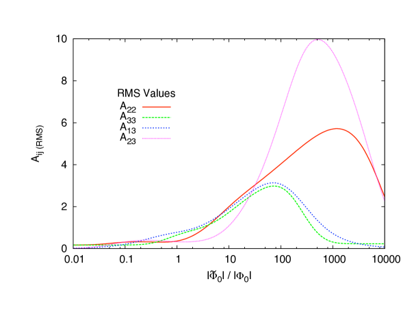
Figure 4: The root mean square (over physical time) of the four leading adiabatic matrix elements $A_{22},A_{33},A_{13}$ and $A_{23}$ computed according to (219). The computation is performed for the modes with momentum $k=0$, for five rotations of the flat direction $\Phi$. While the RMS values are not directly correlated with the growth exponent $\sigma$ shown in Figure 8, they indicate the parameter space where particle production may be possible.

The RMS values of $A_{ij}$ suggest there is indeed a resonance band. One notices that the predicted band is weighted more towards larger values of $|{\tilde{\Phi}}_{0}|/|\Phi_{0}|$ in the figure. This may be explained by the fact that the heavier field ${\tilde{\Phi}}$ becomes unfrozen at a later value of the scale factor than the lighter field $\Phi$ and this results in an effectively smaller ratio $|{\tilde{\Phi}}|/|\Phi|$ once both fields are oscillating. For example, although the ratio is approximately $15$ for the trajectory shown in Figure 29, the effective ratio when both fields are unfrozen and oscillating is clearly closer to unity.

One may now solve the Heisenberg Equations of motion for the same range of parameters to confirm the existence of a resonance band. To obtain some further intuition for the particle production, the total occupation number $n_{tot}=n_{1}+n_{2}+n_{3}$ is shown in Figure 5 compared to the above background evolution. Notice particle production occurs for short periods of time when the fields have comparable magnitude. One may see this feature in the expressions for the elements of the $\Gamma$ matrix (203). The appearance of factors such as $|\Phi|/\sqrt{|\Phi|^{2}+|\tilde{\Phi}|^{2}}$ and $|\tilde{\Phi}|/\sqrt{|\Phi|^{2}+|\tilde{\Phi}|^{2}}$ in these expressions indicate a suppression when the ratio ${\tilde{\Phi}}/\Phi$ is very large or very small, but the $\Gamma$ matrix, and thus particle production, is unsuppressed for those instants when ${\tilde{\Phi}}\sim\Phi$ is obtained. Finally, we should mention that the particle production does not always occur in brief bursts. Specifically, when the fields are continually of a comparable magnitude, the production can then be a more continuous process.

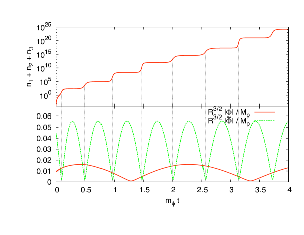
Figure 5: Upper panel: Number density of the produced quanta for a given momentum $k_{*}=10^{-7}\,$. Lower panel: amplitudes of the two flat directions. We note that particle production occurs whenever the two amplitudes are comparable, as discussed in the main text. The parameters chosen for this evolution are $m_{*}=10^{-6},\,F_{*}=2,\,{\tilde{m}}/m=3.72,\,|{\tilde{\Phi}}_{0}|/|\Phi_{0}|=15$

Next we check the rescaling discussed in the previous section. The Heisenberg equations are solved for different values of the parameters $m_{*}$,${\tilde{m}}_{*}$,$\Phi_{0}$, and ${\tilde{\Phi}}_{0}$, and the occupation numbers are rescaled according to (223) in order to compare the spectra at a given time. This procedure is illustrated in Figure 6 where we show the spectrum of the first (heavy) eigenstate for three distinct cases in which the ratio $\frac{m}{M}$ is varied over the range $10^{-7}<\frac{m}{M}<10^{-5}$. The three spectra coincide once $n_{1}$ and $k$ are rescaled according to Table 1. Although we do not show it here, we also verified that the occupation numbers for the light eigenstates do not change with $\frac{m}{M}$.

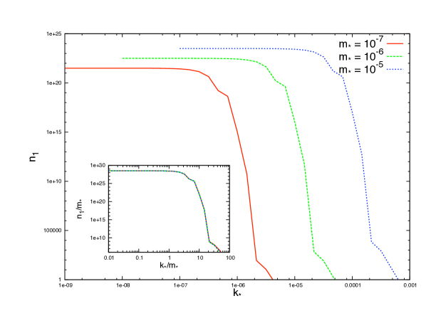
Figure 6: Occupation number for the first (heavy) eigenstate after three rotations of the first direction, for a specific set of parameters: $|\Phi_{0}|=10^{-3}\,M_{p}$, $|{\tilde{\Phi}}_{0}|/|\Phi_{0}|=4$, ${\tilde{m}}/m=3.72$, $\Sigma_{0}=0.25$, ${\tilde{\Sigma}}_{0}=0.156$. The larger figure shows the occupation number as a function of the momentum for three specific choices of the flat direction mass $m_{*}$. The insert shows the same result, but plotting $n_{1}/m_{*}$ vs. $k_{*}/m_{*}$. In terms of these variables, the three curves overlap. Since $m_{*}\propto\frac{m}{M}$, this confirms the scaling (223) for the occupation number, and the fact that the momenta of the quanta produced also scale as $\frac{m}{M}$.

Next the time evolution of $r_{prod}$ is computed, and this is done for three values of the ratio $m/{\tilde{m}}$ and a sampling of the values $|\Phi_{0}|/|{\tilde{\Phi}}_{0}|$ over the resonance bands. The scaling relation (224) is applied to determine the number of rotations at which $r_{prod}=1$ is satisfied with $m=m_{\mathrm{susy}}$ and $M=10^{-2}M_{P}$, and these values are recorded. The results are shown in Figure 7.

The data of Figure 7 exhibits a resonance band for each of the three selected mass ratios. Note also that different values of $\frac{m}{M}$ were used to obtain this data. Thus the figure is a second verification of the scaling relation. Before rescaling there was noticeable scatter in neighboring data points, and after rescaling, the data collapsed to the smooth curves shown in the figure. The growth exponent defined in (226) was also computed for the same parameter set and these are shown in figure 8

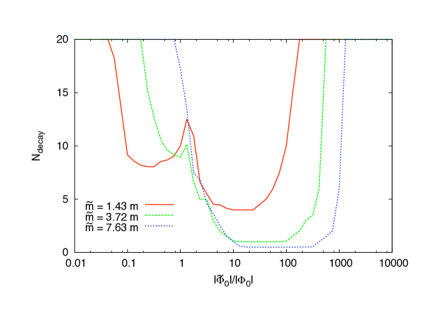
Figure 7: Number of rotations of the first VEV where the production criterion $r_{prod}=1$ is satisfied and its dependence on the initial ratio of the VEVs $|\tilde{\Phi}_{0}|/|\Phi_{0}|$, for three different mass ratios. The numerical analysis was made for the first twenty rotations of the first flat direction and the results were rescaled to $m/e=10^{4}\,{GeV}$ and $\sqrt{|\tilde{\Phi}_{0}|\,|\Phi_{0}|}=10^{-2}M_{p}$.

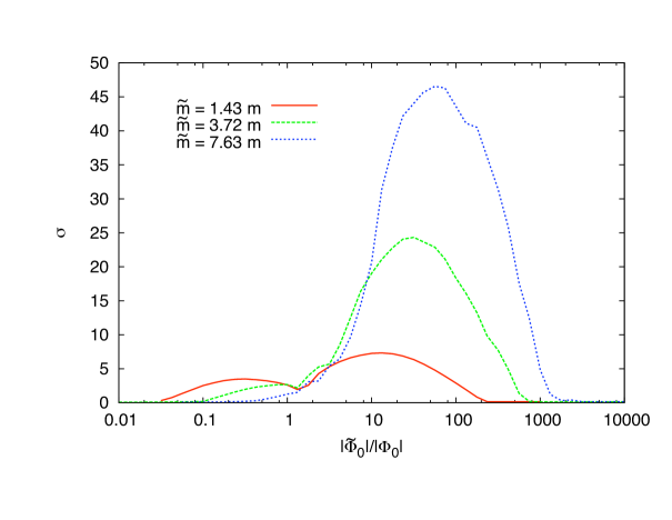
Figure 8: The dependence of the growth exponent $\sigma$ defined in (226) on the initial ratio of the VEVs $|\tilde{\Phi}_{0}|/|\Phi_{0}|$, for three different mass ratios.

The data shown in the Figures 7 and 8 are the main quantitative results of this thesis. They explicitly show the decay of our toy model flat direction for realistic values of the parameter space. The degree to which these results may carry over to MSSM flat directions is discussed in the Conclusions which follow.

Chapter Conclusions

Inflation provides a strong motivation for the study of the dynamics of coherent fields in the early universe. The inflaton itself is a coherent field, and as we have shown, other fields such as supersymmetric flat directions may be made coherent through the process of inflation. The motivation for this thesis and the attempt was to determine the evolution and decay of flat direction VEVs in the early universe. As discussed, the VEVs will break at least some of the standard model gauge symmetries and establish an effective vacuum into which the inflaton would decay and in which the inflaton decay products would thermalize. However, evidence was presented that flat direction fields may decay quickly and nonperturbatively, and thus restore the vacuum to a gauge symmetric state perhaps even before the inflaton has decayed. The final thermalization of the inflaton decay products was not studied, but once the gauge symmetric vacuum is restored, existing techniques such as those of [85] would be applicable.

Our study began with a very brief introduction to supersymmetric theories and the scalar potential of these theories. It was shown that the scalar potential – which is a functional of all the scalar fields of ones model – can possess special nonzero combinations of fields for which the potential is exactly zero. These flat directions are the light scalar fields described above. We thus studied the growth of the fields during inflation, and established reasonable upper bounds on their VEVs as shown in Figure 1. After the conclusion of inflation while the universe is behaving as a matter dominated universe, a special time was noted when the Hubble parameter became comparable to the mass of the light scalar. At this time, the complex scalar would begin to execute well defined oscillation. The motion is generally an elliptic-spiral like trajectory in the complex plane as shown in Figure 2 or 29 with the frequency of rotation being simply the mass of the field. The orientation of rotation and the ellipticity of the trajectory will additionally quantify a conserved charge for the field which in the case of the MSSM flat directions is typically the difference of baryon number and lepton number or $B-L$. During this time both the inflaton and the flat directions both oscillate and reduce in amplitude as matter constituents and as shown in Figure 14. Both will eventually decay however, and the order of their decays is somewhat important. If the inflaton decays first, and into a relativistic species, then the flat direction may overtake the inflaton’s decay products later. However if there are multiple flat directions which have obtained obtained large expectation values, then the flat direction VEVs may decay first through a rapid nonperturbative process.

An example of the nonperturbative decay was shown here. It is shown in a toy $U(1)$ gauge model that the decay can occur in approximately ten or twenty oscillations of the flat direction fields for a range of parameter choices. This is in contrast to the perturbative estimates which would put the flat direction decay to be long after the decay of the inflaton. The Figures 7 and 8 are thus the main quantitative results of this thesis.

In the following we examine some notable aspects of our models. To begin, we note our study [27] was the first concrete calculation of a nonperturbative decay in a gauge model. One consequence of the gauge symmetry on our results has been the gauge current constraint. For instance, in the model of a single flat direction, the gauge current constraint (188) essentially would not admit a time dependent solution except in the circumstance when the masses of the two fields involved were degenerate. We were thus led to select this case in order to consistently apply our formalism. The general case appears to only admit a space-time dependent solution, and to pursue this model apparently would require lattice simulation. Similarly, in the model of multiple flat directions of Section 26 which possesses three flat directions, the gauge current constraint forced one of three flat directions from obtaining a VEV in the solution. A simple lesson from our study is that the current conservation constraint can often have a non-trivial effect on the dynamics. We note that similar conclusions were drawn in the work of [87].

In the above, the conservation of current was considered on just the background. It should be possible to consider gauge current conservation at the level of the perturbations as well. Specifically, the conservation should appear in the Heisenberg Equations of motion. These equations do not conserve current on their own however, so it must be that the driving terms which are derived from the $U(1)$ symmetric Lagrangian will contain this information. Verifying this conservation on the perturbations is another direction which may be pursued.

Having studied the $U(1)$ models, a logical next step would be to pursue the same analysis on an MSSM flat direction. As an example consider again the work of [87] in which the background evolution of the $H_{u}L$ multi-flat direction was solved. These authors obtained only time-dependent solutions to this model. However, using the methods presented in this thesis, the spatial stability may in principle be studied. In particular, for the $H_{u}L$ directions or some other choice of MSSM directions, obtaining the driving terms to the Heisenberg equations would be more involved due to the added gauge symmetry, but the series expansion in the hierarchy $\frac{m}{M}$ for example would greatly facilitate these calculations. In general, the techniques learned by studying the $U(1)$ models here can make these more complicated problems feasible.

Putting aside the above modelling considerations, we consider again the connection between flat direction decay and the equipartition principle which was made in Section 9 and in the Results. The most significant consequence of equipartition is the production of heavy quanta. Our analysis and numerics both revealed that heavy quanta may be produced in the flat direction decay. The production of heavy quanta is not uncommon in preheating scenarios as was discussed for a toy model of inflaton preheating in Section The Evolution and Decay of Supersymmetric Flat Directions in the Early Universe and Their Role in Thermalizing the Universe and has also been shown in more detailed studies (for example [86, 61]). One might speculate that equipartition is a property that all preheating models which involve heavy states might share in common.

However, it is unsettling that states with nearly Planck mass could be produced in such large quantities. One must look to the expected decay time of the heavy quanta to resolve the difficulty. A preliminary estimate of the decay time was made at the conclusion of Section 22 and the estimate indicates a decay time which may be comparable to the mass of the heavy quanta. In order to treat these states consistently as particles, we had to assume the decay time was somewhat longer than one period of oscillation of the heavy state. This time would still be very short compared to the period of a flat direction state, and in particular the ratio of the two periods is simply $\frac{m}{M}$. This suggests the heavy state occupation numbers would be depleted quickly on the time scale of our simulations. Equivalently, this means that the inclusion of interaction terms would be significant for the heavy states. Further study in this area is warranted. However, we note that the exponential production on our model did not greatly rely on the presence of large occupation numbers for the heavy state. This was checked by artificially setting to zero the mixing between the states via $I=J=0$ so that the only source of particle production could be from the evolving eigenfrequencies and not the evolving eigenvectors. After this change, an exponential particle production was still obtained for the light sector of the model.

The above situation in which the final states are short-lived is an interesting one and to our knowledge has not been addressed in the literature. However, the effects of interactions and the back-reaction of produced particles on the condensate have been studied for example in [86], so analysis of a similar nature may be possible. Alternatively, the issue may be resolved through classical lattice simulation. In general, classical lattice simulations may be useful to compare against the generic results obtained here. For instance, classical stability analysis such as the determination of lyapunov exponents may be applied in combination with a lattice simulation [91]. In principle, methods such as these may provide further insight.

Finally, we present some discussion of observables. Our model suffers in this respect in the same way as other models of preheating. The difficulty lies in the process of thermalization itself which erases most all information about what happened during the reheating process aside from gross thermodynamic quantities such as the baryon asymmetry and the reheating temperature. However other observables may survive the reheating process. These include such effects as modulation of the cosmological perturbations, gravitational waves, the creation of dark matter, primordial black holes and topological defects [63]. The most likely place one may look for a signature of the existence of a flat direction VEV may be in the statistics of the cosmological perturbations and in particular the imprint left on the Cosmic Microwave Background. In some specific models known as D-term inflation in which the inflaton is supersymmetric (see [7] for an introduction), it has been noted the flat direction VEVs may contribute to the cosmological perturbations [92, 22]. For instance, bounds may be placed on the magnitude of the flat direction VEV (based on the COBE normalization) which are in the vicinity of $10^{-3}M_{P}$ to $10^{-2}M_{P}$ and which correspond to a lowest non-vanishing terms in the superpotential $n=4$ and $n=6$ [92]. For comparison, see Figure 1. More recently, it has been suggested that the effect of parametric resonance of a field coupled to the flat direction may generically amplify the perturbations of this field so they may be observable in the CMB as curvature perturbations [93]. Again, in the absence of a direct signature, one may constrain proposed models based on non-observation of such a signal [93]. We note this last work appears to have been somewhat motivated by our own work on which this thesis is based [27].

This completes the main body of this thesis on the dynamics of supersymmetric flat directions. While much has been determined in this study, we have emphasized in the above that there remains more work that can be done on this interesting subject.

Chapter Notation

The notation used in the thesis is here summarized for the convenience of both specialist and non-specialist readers.

The notation for fields is as follows: Fundamental complex scalar fields (specifically the fields of which the flat directions are composed) are denoted by $\phi_{i}=f_{i}e^{\sigma_{i}}$ with $i$ running over the whole set of fields. However, the inflaton field is denoted by $\chi$ (the author apologizes as this is an unusual convention). The U(1) vector field is denoted by $B_{\mu}$. The SU(2) and SU(3) vector fields are $A^{a}_{\mu}$, where $a$ is a group index, and it should be clear from the context which symmetry is being considered. Fermions are denoted by $\psi$.

The fundamental fields are typically decomposed into a classical background plus quantized fluctuations away from this background. The classical backgrounds are written in upper case and the perturbations in lower case. In the case of the vector, the classical background is written in calligraphic letters, for instance $B_{\mu}={\cal B}_{\mu}+b_{\mu}$ where $b_{\mu}$ are the quantized fluctuations. Note the background value of the vector ${\cal B}_{\mu}$ is always zero in the context of this thesis (See Section The Evolution and Decay of Supersymmetric Flat Directions in the Early Universe and Their Role in Thermalizing the Universe). Finally, the notation for derivatives is, $\frac{d\chi}{dx^{\mu}}\equiv(\partial_{\mu}\chi)^{2}\equiv(\chi,_{\mu})^{2}$

When discussing the classical background of the scalar fields $\Phi_{i}$, the terms Vacuum Expectation Value (VEV) or scalar condensate are sometimes used as these are equivalent descriptions. When the term VEV is used, it is implied that it is the VEV determined by a local observer in some causally connected patch of the universe at some time, $\langle\phi_{i}\rangle_{\mathrm{patch}}\equiv\Phi_{i}$, and this is not to be confused with the VEV determined over “all” space which is zero $\langle\phi_{i}\rangle_{\mathrm{all\;space}}=0$. We sometimes use the term “Flat Direction” when referring to the VEV, although strictly speaking the flat direction is a property of the scalar potential while the VEV is a realization of the field configuration on the potential (see Section The Evolution and Decay of Supersymmetric Flat Directions in the Early Universe and Their Role in Thermalizing the Universe). Effective vacuum and Bose Einstein condensate are also used to describe the classical background.

In describing the “decay” of the flat direction condensate, we sometimes refer to this as “decoherence” or “the development of spatial instability” as these are all equivalent statements for the decay in the context of our models.

The notation for energy scales is as follows: The mass of the scalar fields which comprise the flat directions will be $m$ or ${\tilde{m}}$ and these will always be of order $m_{\mathrm{susy}}\sim\mathrm{TeV}=1000\,\mathrm{GeV}$ which is the assumed scale of the supersymmetric particle spectrum. The $\mathrm{TeV}$ energy scale (approximately 1000 times the mass of the proton) is heavy by the standards of nuclear and particle physics, but it is relatively light compared to other scales in Cosmology such as the Grand Unified Scale, $M_{\mathrm{GUT}}\sim 10^{16}\,\mathrm{GeV}$ or the Planck scale, $M_{P}\sim 10^{19}\,\mathrm{GeV}$. Note the Planck mass is defined by $G_{N}=\frac{1}{M_{P}^{2}}$. This is not to be confused with the reduced Planck mass $M_{P}^{*}=M_{P}/\sqrt{8\pi}\approx 2.4\times 10^{18}\,\mathrm{GeV}$ which is not used in the thesis. An arbitrary heavy mass scale will be written as $M$, and in the results section $M$ is defined specifically as the scale of the VEVs $|\Phi_{i}|\sim 10^{-2}M_{P}$. The ratio of the $\mathrm{TeV}$ scale states to one of these heavy scales is then generically written $\frac{m}{M}$. A quantity is unsuppressed when it is zeroth order in the expansion in $\frac{m}{M}$.

The gauge couplings are denoted by $"g"$ in Section The Evolution and Decay of Supersymmetric Flat Directions in the Early Universe and Their Role in Thermalizing the Universe where supersymmetry is discussed, but in our model and results sections The Evolution and Decay of Supersymmetric Flat Directions in the Early Universe and Their Role in Thermalizing the Universe and The Evolution and Decay of Supersymmetric Flat Directions in the Early Universe and Their Role in Thermalizing the Universe, we instead use $e$. This is not the electron’s charge as it would be in Quantum Electrodynamics, but the notation is convenient.

The terms parametric resonance, non-adiabatic evolution and nonperturbative dynamics are often used interchangeably.

Finally, the general metric tensor is $g_{\mu\nu}$ and the Minkowski metric tensor is $\eta_{\mu\nu}$. The cosmological scale factor is $R$. The conformal time is $\eta$ with time derivatives written as a prime (such as $R^{\prime}$), and physical time is $t$ with time derivatives written with a dot (such as $\dot{R}$).

Chapter Details Regarding U(1) Gauge Symmetric Actions

The action for a $U(1)$ gauge field, and $n$ complex scalars charged under this gauge group is presented in the main text (182). The procedure for gauge fixing such actions to the unitary gauge was also presented there. Some details which were not explained in Section The Evolution and Decay of Supersymmetric Flat Directions in the Early Universe and Their Role in Thermalizing the Universe are explained here. In particular, it is shown here (i) how to incorporate the expansion of the universe, (ii) how to decompose the vector field Lagrangian and eliminate the nondynamical time-like component $B_{0}$ and (iii) how to diagonalize the Lagrangians for the systems of two fields and four fields in the expansion parameter $\frac{m}{M}$.

Incorporating the Expansion of the Universe: With a change of spatial coordinates and a rescaling of fields one may put the Lagrangian (182) in a form which is more easily quantized. The background metric is taken to be the Friedmann-Robertson-Walker metric with the spatial curvature constant set to zero. The line element for this metric is $ds^{2}=dt^{2}-R(t)^{2}d{\vec{x}}^{2}$, where $R(t)$ is the scale factor. It is convenient to use the conformal time coordinate $\eta$ which is related to the physical time by $Rd\eta=dt$. The line element in these coordinates is,

$$g_{\mu\nu}dx^{\mu}dx^{\nu}=R(t)^{2}\eta_{\mu\nu}dx^{\mu}dx^{\nu}=R(t)^{2}(dt^{2}-d{\vec{x}}^{2})$$

where $\eta_{\mu\nu}$ is the Minkowski metric. After choosing the conformal time, the action (182) is written in a way that the raising and lowering of the space-time indeces is simply done with the minkowski metric as follows,

$$S=\int d^{4}xR^{4}\left\{-\frac{1}{4R^{4}}\eta^{\mu\mu^{\prime}}\eta^{\nu\nu^{\prime}}F_{\mu\nu}F_{\mu^{\prime}\nu^{\prime}}+\frac{1}{R^{2}}\eta^{\mu\nu}(D_{\mu}\phi_{i})(D_{\nu}\phi_{i})^{*}-V(\phi_{1},...\phi_{n})\right\}$$

Additionally, if we redefine the scalar fields $\phi=\frac{\varphi}{R}$, the action rewrites,

$$S=\int d^{4}x\left\{-F_{\mu\nu}F^{\mu\nu}+(D_{\mu}\varphi_{i})(D^{\mu}\varphi_{i})^{*}+\frac{R^{\prime\prime}}{R}\varphi_{i}^{2}-R^{4}V\left(\frac{\varphi_{1}}{R},...\frac{\varphi_{n}}{R}\right)\right\}$$

where primes above denote $\frac{\partial}{\partial\eta}$ where the scale factor now appears through the effective mass term and also may appear in the potential, though the potentials we consider such as that from the D-term are quartic in the scalar fields, and so $R^{4}\phi^{4}=\varphi^{4}$ and the scale factor drops from these terms as well. To summarize, for the Lagrangians (182), the prescription for incorporating the scale factor is to replace the mass terms as follows

$$m_{i}^{2}\phi^{2}\rightarrow\left(R^{2}m^{2}_{i}-\frac{R^{\prime\prime}}{R}\right)\varphi_{i}^{2}$$

and when later computing physical quantities to convert back to comoving coordinates via $Rd\eta=dt$ and to physical fields via $\phi_{i}=\frac{\varphi}{R}$.

Decomposing the Vector Field and Eliminating the Nondynamical Time-like Component: We now decompose the vector field in our U(1) actions (182). We note that $B_{\mu}$ is coupled to the scalars through the current $J^{\mu}$ as well as through the effective mass term ${\cal M}^{2}$ both defined in (184). The part of the lagrangian which contains the vector is thus,

$$-\frac{1}{4}F(B)^{2}+\frac{1}{2}{\cal M}^{2}B_{\mu}B^{\mu}-B_{\mu}J^{\mu}$$

where the field strength tensor is $F_{\mu\nu}=\partial_{\mu}B_{\nu}-\partial_{\nu}B_{\mu}$. We split $B_{\mu}$ into it’s space and time components $B_{0}$ and $B_{i}$ as follows

$$\mathcal{L}_{massless} = -\frac{1}{4}F_{\mu\nu}F^{\mu\nu}$$

$$= -\frac{1}{2}F_{0i}F^{0i}-\frac{1}{4}F_{ij}F^{ij}$$

$$= \frac{1}{2}F_{0i}F_{0i}-\frac{1}{4}F_{ij}F_{ij}$$

$$= \frac{1}{2}\left(B_{i},_{0}-B_{0},_{i}\right)^{2}-\frac{1}{4}\left(B_{j},_{i}-B_{i},_{j}\right)^{2}$$

$$= \frac{1}{2}B_{i}^{\prime}B_{i}^{\prime}+\frac{1}{2}B_{0},_{i}B_{0},_{i}-B_{i}^{\prime}B_{0},_{i}-\frac{1}{2}B_{j},_{i}B_{j},_{i}+\frac{1}{2}B_{j},_{i}B_{i},_{j}$$

$$= \frac{1}{2}B^{i\prime}B^{i\prime}+\frac{1}{2}B^{0},_{i}B^{0},_{i}+B^{i\prime}B^{0},_{i}-\frac{1}{2}B^{j},_{i}B^{j},_{i}+\frac{1}{2}B^{j},_{i}B^{i},_{j}$$

$$= \frac{1}{2}{\vec{B}}^{\prime}\cdot{\vec{B}}^{\prime}+\frac{1}{2}\nabla B_{0}\cdot\nabla B_{0}+{\vec{B}}^{\prime}\cdot\nabla B_{0}-\frac{1}{2}|\nabla\times\vec{B}|^{2}$$

where the identity $\epsilon_{ijk}\epsilon_{ilm}=(\delta_{jl}\delta_{km}-\delta_{jm}\delta_{kl})$ has been applied. The Lagrangian for the massive vector field is then

$${\cal L}=\frac{1}{2}\left\{\begin{array}[]{l}|{\vec{B}}^{\prime}|^{2}+|\nabla B_{0}|^{2}+2{\vec{B}}^{\prime}\cdot\nabla B_{0}-|\nabla\times\vec{B}|^{2}\\[3.99994pt] +\;{\cal M}^{2}(B_{0}^{2}-|\vec{B}|^{2})-2J_{0}B_{0}+2\vec{J}\cdot\vec{B}\end{array}\right\}$$ (228)

We split the vector into a transverse and longitudinal part $\vec{B}={\vec{B}}_{T}+\nabla L$ where $\nabla\cdot{\vec{B}}_{T}=0$. The transverse part of the vector decouples from the Lagrangian since it transforms under the Lorentz group as a spin-1 field, while the scalar longitudinal mode of the vector as well as the fundamental scalar fields transform as Lorentz scalars. Hence the transverse mode will decouple at quadratic order in the perturbations. We thus only consider the longitudinal mode $\nabla L$ as well as $B_{0}$ which is non dynamical and will be replaced by substitution of its equation of motion. The equations of motion for $B_{\mu}$ are

$$F_{\mu\nu},^{\mu}+{\cal M}^{2}B_{\nu} = j_{\mu}$$

$$\Box B_{\nu}-(B_{\mu},^{\mu}),_{\nu}+{\cal M}^{2}B_{\nu} = j_{\mu}$$

and from these, the equations of motion for $B_{0}$ and $B_{i}$ are,

$$-\nabla^{2}B_{0}-\partial_{t}(\nabla\cdot\vec{B})+{\cal M}^{2}B_{0} = J_{0}$$ (229)

$$-\Box\vec{B}-\nabla(\partial_{0}B_{0}-\nabla\cdot\vec{B})-{\cal M}^{2}\vec{B} = \vec{J}$$ (230)

We solve for $B_{0}$ by inverting the equation,

$$(-\nabla^{2}+{\cal M}^{2})B_{0} = J_{0}+(\nabla^{2}L^{\prime})$$

The part of the Lagrangian (228) corresponding to the longitudinal mode is then determined to be,

$$\frac{1}{2}\left\{|\nabla L^{\prime}|^{2}-B_{0}\left[J_{0}+\nabla^{2}L^{\prime}\right]-{\cal M}^{2}|\nabla L|^{2}+2\vec{J}\cdot\nabla L\right\}$$ (231)

The remaining aspects of the calculation will be done in momentum space for which the expression for $B_{0}$ is,

$$B_{0}=\frac{J_{0}-k^{2}L^{\prime}}{k^{2}+{\cal M}^{2}}$$ (232)

where $k=|\vec{k}|$, The longitudinal part of the Lagrangian (231) in momentum space is,

$$\frac{1}{2}\left\{\left(\frac{k^{2}{\cal M}^{2}}{k^{2}+{\cal M}^{2}}\right){L^{*}}^{\prime}L^{\prime}+\frac{k^{2}(J_{0}^{*}L^{\prime}+J_{0}{L^{*}}^{\prime})}{k^{2}+{\cal M}^{2}}-\frac{J^{*}_{0}J_{0}}{k^{2}+{\cal M}^{2}}\right.$$

$$\left.-\;{\cal M}^{2}k^{2}L^{*}L+({\vec{J}}^{*}L+{\vec{J}}L^{*})\cdot\vec{k}\right\}$$ (233)

The longitudinal mode can then be made canonical with the field redefinition,

$$L=\left(\frac{\sqrt{k^{2}+{\cal M}^{2}}}{k{\cal M}}\right)\hat{L}$$ (234)

Notice in the simple case where the current is exactly zero, the Lagrangian for the longitudinal mode of the vector after applying the field redefinition is,

$$\frac{1}{2}\left\{{\hat{L}}^{*\prime}{\hat{L}}^{\prime}-({\cal M}^{2}+k^{2}){\hat{L}}^{*}{\hat{L}}\right\}$$ (235)

which is the expected result for a freely propagating longitudinal mode of the massive vector field. The above normalization (234) will be performed on the specific examples which follow in the case of nonzero current $J_{0}$. The longitudinal mode should still obtain the above dispersion relation $\omega^{2}=k^{2}+{\cal M}^{2}$ when the fields are evolving adiabatically.

To this point the Lagrangian has been written in the fundamental field description. However for the purpose of computing observables, the Lagrangians are always expressed in background fields plus perturbations. The models we are interested in have backgrounds which satisfy $\langle B_{\mu}\rangle=0$ and also $\langle J_{0}\rangle=0$, so we must only consider the linear perturbations in these quantities, $b_{\mu}$ and $j_{\mu}$ in order to obtain a quadratic Lagrangian from the above result (233). Additionally, we will employ the expansion parameter $\frac{m}{M}$ which was also applied in Section 9. Our objective is to obtain the quantities $\Gamma_{ij}$ and $\omega_{i}$ to leading order in this expansion.

Diagonalization of the Two field Model: The Lagrangian for the perturbations is (193) from which we read the current density and effective mass of the vector to be,

$$j_{0}=\frac{1}{2}eF\Sigma^{\prime}\delta\;\;\;,\;\;\;\vec{j}=0$$

$${\cal M}=\frac{1}{2}eF$$

The Lagrangian (193) after the elimination of $b_{0}$ is,

$$\frac{1}{2}\left[(\partial_{\mu}f)^{2}+(\partial_{\mu}\sigma)^{2}+(\partial_{\mu}\delta)^{2}\right]+\frac{1}{2}\Sigma^{\prime}\left(f\sigma^{\prime}-f^{\prime}\sigma\right)$$

$$-\;\frac{1}{2}\left(m_{+}^{2}-\frac{1}{4}\Sigma^{\prime 2}\right)f^{2}-\frac{1}{2}\left(m_{+}^{2}-\frac{1}{4}\Sigma^{\prime 2}\right)\sigma^{2}$$

$$-\;\frac{1}{2}\left(\frac{1}{4}{e}^{2}F^{2}+m_{+}^{2}+\frac{3}{4}\Sigma^{\prime 2}\right)\delta^{2}$$ (236)

where the vector field is not shown since it has been decoupled. The remaining coupled system involves $f$ and $\sigma$ and these fields are obtained to be degenerate in mass $m$. They are simply the flat direction perturbations.

Diagonalization of the Four Field Model: In the four field model, the current density of (195) and the effective vector mass are obtained in terms of the perturbations (200) to be,

$$j_{0}=e\left[(F^{2}-G^{2})\theta^{\prime}+2F\Sigma^{\prime}\delta+2G{\tilde{\Sigma}}^{\prime}{\tilde{\delta}}\right]$$

$$\vec{j}=e(F^{2}-G^{2})\nabla\theta$$

$${\cal M}=e\sqrt{F^{2}+G^{2}}$$

Substituting these into (233), one notices there will be coupling between $L$ and $\theta$ in their kinetic terms at leading order. Our procedure will be to first find the transformation which makes these kinetic terms canonical (temporarily discarding mass terms and mixed terms). We then apply this transformation to obtain the complete Lagrangian in the form (69). The kinetic terms are,

$$\frac{1}{2}\left\{{\hat{L}}^{*\prime}{\hat{L}}^{\prime}+\frac{k}{\sqrt{k^{2}+{\cal M}^{2}}}\left(\frac{j_{0}^{*}}{{\cal M}}{\hat{L}}^{\prime}+\frac{j_{0}}{{\cal M}}{\hat{L}}^{*\prime}\right)-\frac{\left(\frac{|j_{0}|}{{\cal M}}\right)^{2}}{1+\left(\frac{k}{{\cal M}}\right)^{2}}+(F^{2}+G^{2}){\theta^{*}}^{\prime}\theta^{\prime}\right\}$$

$$= \frac{1}{2}\left\{{\hat{L}}^{*\prime}{\hat{L}}^{\prime}+{\hat{\theta}}^{*\prime}{\hat{\theta}}^{\prime}+\frac{k}{{\cal M}}\frac{F^{2}-G^{2}}{\sqrt{4F^{2}G^{2}+(F^{2}+G^{2})^{2}\left(\frac{k}{{\cal M}}\right)^{2}}}({\hat{\theta}}^{*\prime}{\hat{L}}^{\prime}+{\hat{\theta}}^{\prime}{\hat{L}}^{*\prime})\right\}$$

where $j_{0}$ has been substituted and the kinetic term for $\theta$ has been normalized. This last expression is compactly written in matrix notation in terms of the fields $L$ and $\theta$ as follows,

$$\frac{1}{2}(L^{*},\theta^{*})^{\prime}\left[\begin{array}[]{ll}n_{L}&0\\ 0&n_{\theta}\end{array}\right]\left[\begin{array}[]{ll}1&Q\\ Q&1\end{array}\right]\left[\begin{array}[]{ll}n_{L}&0\\ 0&n_{\theta}\end{array}\right]\left(\begin{array}[]{l}L\\ \theta\end{array}\right)^{\prime}$$

where

$$Q = \frac{k}{{\cal M}}\frac{F^{2}-G^{2}}{\sqrt{4F^{2}G^{2}+(F^{2}+G^{2})^{2}\left(\frac{k}{{\cal M}}\right)^{2}}}$$

$$n_{\theta} = \sqrt{\frac{4F^{2}G^{2}+(F^{2}+G^{2})^{2}\left(\frac{k}{{\cal M}}\right)^{2}}{(F^{2}+G^{2})(1+\left(\frac{k}{{\cal M}}\right)^{2})}}$$

$$n_{L} = \frac{k{\cal M}}{\sqrt{k^{2}+{\cal M}^{2}}}$$

One may apply the following additional rotations and rescalings,

$$\left(\begin{array}[]{l}L_{c}\\ \theta_{c}\end{array}\right)=R_{1}^{T}R_{0}^{T}\left[\begin{array}[]{ll}\sqrt{1+Q}&0\\ 0&\sqrt{1-Q}\end{array}\right]R_{0}\left[\begin{array}[]{ll}n_{L}&0\\ 0&n_{\theta}\end{array}\right]\left(\begin{array}[]{l}L\\ \theta\end{array}\right)$$ (238)

where $R_{0}$ is a time independent rotation and $R_{1}$ is a small time dependent rotation,

$$R_{0} = \frac{1}{\sqrt{2}}\left(\begin{array}[]{ll}1&1\\ -1&1\end{array}\right)$$

$$R_{1} = \left[\begin{array}[]{ll}1-\frac{k^{2}q^{2}}{2}&kq\\ -kq&1-\frac{k^{2}q^{2}}{2}\end{array}\right]$$

$$q = \frac{-F^{2}+G^{2}}{4eFG\sqrt{F^{2}+G^{2}}}$$

and these rotations have been chosen specifically to decouple the longitudinal mode of the vector from the other scalar degrees of freedom. The expression (238) may be inverted and expanded finally to obtain,

$$\theta = \frac{\sqrt{F^{2}+G^{2}}}{2FG}\theta_{c}+{\cal O}\left(\frac{m^{3}}{M^{3}}\right)$$ (241)

$$L = \frac{L_{c}}{k}-\frac{(F^{2}-G^{2})}{2eFG\sqrt{F^{2}+G^{2}}}\theta_{c}+\frac{k}{2{e}^{2}(F^{2}+G^{2})}L_{c}+{\cal O}\left(\frac{m^{2}}{M^{2}}\right)$$ (242)

This final result is substituted into the Lagrangian (233). The remaining mixed scalar degrees of freedom are arranged in a vector $X=(\delta,{\tilde{\delta}},\theta_{c})$, and the Lagrangian for these has the desired form (68). Specifically, the $K$ matrix, the matrix $({\tilde{\Omega}}^{2}+K^{T}K)$, the eigenvalues $\omega_{i}$ and the matrix $\Gamma$ are all shown in the main text (201-203).

Chapter Calculating the Variance of a Scalar Test Field During Inflation

We determine the variance of test scalar field $\phi$ during an asymptotically de Sitter expansion. The sampling is done inside a patch of space of width $L$. We are not interested in wavelengths smaller than $L$, so we smear out these fast fluctuations by use of a window function $W_{L}(x)$,

$$\phi_{L}(t)=\int d^{3}xW_{L}(x)\phi(x,t)\;\;\;\;,\;\;\;\;W_{L}(x)=\frac{1}{(2\pi)^{3/2}L^{3}}e^{-\frac{x^{2}}{2L^{2}}}$$ (243)

in which $W_{L}(x)$ is any reasonable normalized distribution of order 1 inside the patch, and dropping to zero quickly outside of the patch. In the above, it is taken to be a normalized Gaussian. The quantity $\phi_{L}$ is then the quantity which we must determine the variance of. The calculation is performed using conformal time $dt=Rd\eta$, and a redefined scalar field $\phi=\frac{\varphi}{R}$. The fields are decomposed as in (106), and the variance is thus obtained to be,

$$\langle\varphi_{L}^{2}\rangle = \langle 0|\left[\int d^{3}x\;W_{L}(x)\varphi\right]^{2}|0\rangle$$ (244)

$$= \frac{1}{2}\int\frac{d^{3}k}{(2\pi)^{3}}|h_{k}|^{2}|w(kL)|^{2}$$ (245)

$$\approx \frac{1}{2}\int_{0}^{L^{-1}}\frac{d^{3}k}{(2\pi)^{3}}|h_{k}|^{2}$$ (246)

where $w(kL)$ is the Fourier Transform of the window function, and we’ve used the fact that $w(kL)$ is order 1 for $|k|<L^{-1}$ and drops to zero quickly for $|k|>L^{-1}$. The effect of the window function is simply to impose a momentum cutoff. In the de Sitter metric, the equations for the modes is listed in the main text (111) which again is

$$h_{k}^{\prime\prime}+\left[k^{2}+\left(\frac{m^{2}}{H_{I}^{2}}-2\right)\frac{1}{\eta^{2}}\right]h_{k}=0$$ (247)

and may be put in the form of Bessel’s equation with the definitions $x\equiv-k\eta$, and $h_{k}(\eta)\equiv\sqrt{x}f(x)$,

$$x^{2}\frac{d^{2}f(x)}{dx^{2}}+x\frac{df(x)}{dx}+(x^{2}-n^{2})f(x)=0\;\;\;,\;\;\;n^{2}=\frac{9}{4}-\frac{m^{2}}{H^{2}}$$ (248)

the solutions are, $f(x)=A_{k}J_{n}(x)+B_{k}Y_{n}(x)$, and so the mode functions take the form,

$$h_{k}(\eta)=\sqrt{-k\eta}\left(A_{k}J_{n}(-k\eta)+B_{k}Y_{n}(-k\eta)\right)\;\;\;,\;\;\;n^{2}=\left(\frac{9}{4}-\frac{m^{2}}{H^{2}}\right)$$ (249)

The constants $A_{k}$ and $B_{k}$ must now be determined from the initial conditions for the modes which are fixed by the quantum fluctuations. Technically this means we must canonically normalize the modes $h_{k}$ at early times (or large k). The equation (247) for the modes at sub-horizon scales, asympotes to $h_{k}^{\prime\prime}+k^{2}h_{k}=0$ with solutions $e^{\pm ik\eta}$. Referring to (106), we want $h_{k}(\eta)=\frac{1}{\sqrt{2k}}e^{-ik\eta}$ at early times for our fields to be canonically normalized. Our solutions (249) are then normalized as follows,

$$h_{k}(\eta)=\sqrt{\frac{-\eta\pi}{4}}e^{i\left(\frac{n\pi}{2}+\frac{\pi}{4}\right)}\left(J_{n}(-k\eta)+iY_{n}(-k\eta)\right)$$ (250)

where one may apply the asymptotic form of the Bessell functions which is,

$$\left(J_{n}(-k\eta)+iY_{n}(-k\eta)\right)\sim\sqrt{\frac{2}{\pi(-k\eta)}}e^{i\left(-k\eta-\frac{n\pi}{2}-\frac{\pi}{4}\right)}\;\;\;,\;\;\;\mbox{for large }(-k\eta)$$ (251)

from which it is quick to verify that the solutions (250) have the correct asymptotic form far within the horizon. We consider these solutions in the limit of small mass $\frac{m}{H_{I}}<1$ where $n^{2}>0$, and large mass $\frac{m}{H_{I}}>1$ where $n^{2}<0$, and we note the Bessell solutions will still hold in the latter case when $n$ is pure imaginary. We are interested in calculating the variance, so we substitute in our general solution, and we approximate our solutions in the long wavelength limit as our integration will only be over scales larger than the horizon. The steps of the calculation are shown first for the case $n^{2}>0$,

$$\langle\varphi_{L}(\eta)^{2}\rangle_{n^{2}>0} \approx \frac{1}{2}\int_{0}^{L^{-1}}\frac{d^{3}k}{(2\pi)^{3}}|h_{k}|^{2}$$

$$\approx \frac{1}{2}\int_{0}^{L^{-1}}\frac{dk}{(2\pi)^{2}}k^{2}\frac{(-\eta\pi)}{4}\left|J_{n}(-k\eta)+iY_{n}(-k\eta)\right|^{2}$$

$$\langle\phi^{2}(t)\rangle_{n^{2}>0} \approx \frac{1}{2}\int_{0}^{L_{phys}^{-1}}\frac{dk_{phys}}{(2\pi)^{2}}\frac{k_{phys}^{2}}{4H_{I}}\left|J_{n}\left(\frac{k_{phys}}{H_{I}}\right)+iY_{n}\left(\frac{k_{phys}}{H_{I}}\right)\right|^{2}$$

$$\approx \frac{1}{2}H_{I}^{2}\int_{0}^{(H_{I}L_{phys})^{-1}}\frac{dx}{(2\pi)^{2}}\frac{x^{2}}{4}\left|J_{n}(x)+iY_{n}(x)\right|^{2}$$

$$\approx \frac{1}{2}H_{I}^{2}\int_{0}^{(H_{I}L_{phys})^{-1}}\frac{dx}{(2\pi)^{2}}\frac{x^{2}}{4}\left|-\frac{2^{n}\Gamma(n)}{\pi}(x)^{-n}\right|^{2}\;\;\;\mbox{for }x\ll 1$$

$$\approx H_{I}^{2}\left(\frac{2^{(2n-5)}\Gamma(n)^{2}}{\pi^{4}}\right)\int_{0}^{(H_{I}L_{phys})^{-1}}\frac{dx}{x}x^{(3-2n)}$$

where we have put the expression in terms of the physical momenta, $k=k_{phys}R$, and original fields $\phi=\varphi/R$, then put the integration over the dimensionless variable $x=\frac{k_{phys}}{H_{I}}$. We may similarly calculate the case $n^{2}<0$,

$$\langle\varphi_{L}(\eta)^{2}\rangle_{n^{2}<0} \approx \frac{1}{2}\int_{0}^{L^{-1}}\frac{d^{3}k}{(2\pi)^{3}}|h_{k}|^{2}$$

$$\approx \frac{1}{2}\int_{0}^{L^{-1}}\frac{dk}{(2\pi)^{2}}k^{2}\frac{(-\eta\pi)}{4}e^{-|n|\pi}\left|J_{i|n|}(-k\eta)+iY_{i|n|}(-k\eta)\right|^{2}$$

$$\langle\phi^{2}(t)\rangle_{n^{2}<0} \approx \frac{1}{2}\int_{0}^{L_{phys}^{-1}}\frac{dk_{phys}}{(2\pi)^{2}}\frac{k_{phys}^{2}}{4H_{I}}e^{-|n|\pi}\left|J_{i|n|}\left(\frac{k_{phys}}{H_{I}}\right)+iY_{i|n|}\left(\frac{k_{phys}}{H_{I}}\right)\right|^{2}$$

$$\approx \frac{1}{2}H_{I}^{2}\int_{0}^{(H_{I}L_{phys})^{-1}}\frac{dx}{(2\pi)^{2}}\frac{x^{2}}{4}e^{-|n|\pi}\left|J_{i|n|}(x)+iY_{i|n|}(x)\right|^{2}$$

$$\approx H_{I}^{2}\left(\frac{1}{16|n|\pi^{3}}\right)\int_{0}^{(H_{I}L_{phys})^{-1}}\frac{dx}{x}x^{3}\;\;\;\mbox{for }n\approx\frac{m}{H_{I}}\mg 1$$

Chapter Inflaton Oscillations After Inflation

Here, the approximate evolution of the inflaton field at the conclusion of inflation is determined in the case of a quadratic inflaton potential. Note, the result has been used in (121) of the main text. Also note that the approximate evolution of the flat direction fields (124) used in the main text may be determined through a similar method as that shown below for the inflaton (see also [20]).

To begin, the Friedmann equation and the equation of motion for the dominating isotropic and homogeneous inflaton field are,

$$H^{2}=\left(\frac{\dot{s}}{s}\right)^{2}=\frac{8\pi G}{3}\left(\frac{1}{2}{\dot{\chi}}^{2}+V(\chi)\right)$$ (252)

$$\ddot{\chi}+3H\dot{\chi}+\frac{dV}{d\chi}=0\hskip 20.00003pt\mbox{ where }\hskip 20.00003ptV=\frac{1}{2}m^{2}\chi^{2}$$ (253)

At late times, after inflation as occurred, this field is oscillating around the minimum of its potential $(V=0,\chi=0)$. The motion is determined by the above equations, and one assumes a solution of damped oscillations,

$$\chi(\tau)=X(\tau)\sin[m\tau]\hskip 40.00006ptX(\tau)=\frac{A_{1}}{\tau}+\frac{A_{3}}{\tau^{3}}+...$$ (254)

where we’ve defined the time parameter $\tau=(t-t_{0})$ with $t_{0}$ being the onset of the inflaton oscillations. Specifically, $\dot{\chi}(\tau=0)=0$ and this constraint requires $X(\tau)$ must not contain even powered terms. We may solve for the series $A_{1},A_{3},...$ by an iterative procedure. Substitute the trial solution into (252), and set $A_{1}=A$. Also set $\sin mt=s$ and $\cos mt=c$ to simplify the notation,

$$\dot{X} = -At^{-2}+O(t^{-4})$$

$$\ddot{X} = 2At^{-3}+O(t^{-5})$$

$$\dot{\chi} = {\dot{X}}s+mXc$$ (255)

$$= Ast^{-2}+mcAt^{-1}$$

$$\ddot{\chi} = \ddot{X}s+2m\dot{X}c-m^{2}Xs$$ (256)

$$= -2mcAt^{-2}-m^{2}Ast^{-1}$$

where only the lowest order terms have been retained. Then, from (252),

$$H^{2} = \frac{4\pi G}{3}\left(({\dot{X}}s+mXc)^{2}+m^{2}X^{2}s^{2}\right)$$ (257)

$$= \frac{4\pi G}{3}\left(m^{2}X^{2}(s^{2}+c^{2})+2m{\dot{X}}Xsc\right)$$

$$= \frac{4\pi G}{3}m^{2}X^{2}\left(1+2sc\frac{\dot{X}}{mX}\right)$$

$$= \frac{4\pi G}{3}m^{2}\frac{A^{2}}{t^{2}}\left(1-\frac{2sc}{mt}\right)$$

Now substitute for $\dot{\chi}$, $\ddot{\chi}$ and $H$ into (253) and keep track of the order $t^{-n}$.

$$0 = \ddot{\chi}+3H\dot{\chi}+m^{2}\chi$$

$$0 = (-2mct^{-2}-m^{2}Ast^{-1}+O(t^{-3}))$$

$$+\;3\left(\left[\frac{4}{3}\pi Gm^{2}\right]^{1/2}At^{-1}+O(t^{-3/2})\right)(Ast^{-2}+mcAt^{-1})$$

$$+\;m^{2}s(At^{-1}+O(t^{-3}))$$

$$0 = (-m^{2}As+m^{2}As)t^{-1}+\left(-2mcA+3mcA^{2}\left[\frac{4}{3}\pi Gm^{2}\right]^{1/2}\right)t^{-2}+O(t^{3})$$

the first term vanishes, indicating that the guess for the solution was correct, and the condition for the second term to vanish fixes the constant $A$,

$$A=A_{1}=\frac{1}{\sqrt{3\pi Gm^{2}}}$$ (258)

Considering higher order terms would yield the coefficients $A_{3},A_{5},...$, which will not be done. Substituting (258) into (257) yields the Hubble parameter to lowest order,

$$H\approx\frac{2}{3t}$$ (259)

which is the Hubble parameter of a perfect fluid of nonrelativistic and pressureless matter.

Chapter Thermodynamics of a Relativistic Plasma

Here we present some expressions used in the main text for a universe dominated by an isotropic and homogenous relativistic fluid in thermal equilibrium. First, the total energy density of the fluid is related to the temperature through the Stefan-Boltzman Law,

$$\rho\approx\rho_{rad}=\frac{\pi^{2}}{30}g_{*}T_{rad}^{4}\;\;\;,\;\;\;g_{*}(T)=g_{b}+\frac{7}{8}g_{f}$$

where $g_{*}$ is the effective number of degrees of freedom in the fluid and $g_{b}$ and $g_{f}$ are the numbers of bosonic and fermionic degrees of freedom respectively. Using the Stefan-Boltzman law in combination with the Friedmann equation, one determines the temperature in terms of the Hubble parameter,

$$\rho_{rad} = \frac{3M_{p}^{2}}{8\pi}H^{2}$$

$$\frac{\pi^{2}}{30}g_{*}T^{4} = \frac{3M_{p}^{2}}{8\pi}H^{2}$$

$$T = \left(\frac{45M_{p}^{2}}{4g_{*}\pi^{3}}\right)^{1/4}H^{1/2}$$ (260)

$$= \left(\frac{45}{4g_{*}\pi^{3}}\right)^{1/4}\sqrt{HM_{P}}$$

The entropy density for this relativistic fluid may be determined to be,

$$s=\frac{2\pi^{2}}{45}g_{*}T^{3}$$

The entropy density may then be written in terms of the energy density using the Stefan Boltzman Law,

$$s = \frac{2\pi^{2}}{45}g_{*}\left(\frac{30\rho_{rad}}{g_{*}\pi^{2}}\right)^{3/4}$$ (261)

$$= \frac{2\pi^{1/2}}{45}(30)^{3/4}g_{*}^{1/4}\rho_{rad}^{3/4}$$

$$\approx \rho_{rad}^{3/4}$$

Finally, the number density of a component relativistic species $X$ is,

$$n_{X}=\frac{\zeta(3)}{\pi^{2}}g_{X}T^{3}\hskip 40.00006pt\zeta(3)\approx 1.2$$

where $\zeta$ is the Riemann zeta function.

Chapter Determination of Various Scale Factors and Events

We determine some expressions used in the main text which involve the scale factor at different events during the evolution of the inflaton and flat direction. The reader is referred to Figure 14 as well as to the following table which describes the succession of events with $R$ increasing as one moves down the table from the top.

Event	$\mathbf{R}$	Eq. of state
inflaton begins oscillations	$R_{0}$
		matter dom
flat direction begins to oscillate	$R_{m}$
inflaton decays	$R_{d\chi}$	——
		radiation dom
flat direction overtakes inflaton	$R_{eq}$	——
		matter dom

Other scale factors not shown in the table are $R_{d\Phi}$, the scale factor at the instant of flat direction decay and $R_{RH}$, the scale factor at the instant of thermalization. Only the ratios of scale factors are physically meaningful and to determine any ratio, we can apply the following relations,

$$R\propto t^{2/3}\;\;\;\rightarrow\;\;\;t\propto H^{-1}\;\;\;\rightarrow\;\;\; R\propto H^{-2/3}$$ during matter domination

$$R\propto t^{1/2}\;\;\;\rightarrow\;\;\;t\propto H^{-1}\;\;\;\rightarrow\;\;\; R\propto H^{-1/2}$$ during radiation domination

and we will also need to know the energy densities of the flat direction to the inflaton at some reference times which we will take to be the onset of their respective oscillations.

$$r_{\chi}\equiv\frac{\rho_{\chi_{0}}}{m_{\chi}^{2}M_{P}^{2}}\;\;\;,\;\;\;r_{\Phi}\equiv\frac{\rho_{\Phi_{m}}}{m^{2}\Phi_{0}^{2}}\;\;\;,\;\;\;r_{m}\equiv\left(\frac{\rho_{\Phi}}{\rho_{\chi}}\right)_{m}=\frac{r_{\Phi}}{r_{\chi}}\left(\frac{\Phi_{0}}{M_{P}}\right)^{2}$$

where the last expression is the ratio of the energy densities at the onset of flat direction oscillations. For example, using the above tools, the energy density of the inflaton at the instant of inflaton decay is obtained,

$$\rho_{\Gamma_{\chi}}\sim r_{\chi}(\Gamma_{\chi}M_{P})^{2}$$

Similarly, the scale factor when the flat direction overtakes the inflaton $R_{eq}$ is obtained,

$$\frac{\rho_{\Phi}}{\rho_{\chi}} \sim 1$$

$$\frac{\rho^{m}_{\Phi}\left(\frac{R_{m}}{R_{eq}}\right)^{3}}{\rho_{\chi}^{m}\left(\frac{R_{m}}{R_{d\chi}}\right)^{3}\left(\frac{R_{d\chi}}{R_{eq}}\right)^{4}} \sim 1$$

$$\frac{R_{eq}}{R_{d\chi}} \sim \frac{1}{r_{m}}$$ (262)

which is valid for $r_{m}<1$. The condition for which the flat direction dominates is,

$$\frac{R_{eq}}{R_{d\Phi}} < 1$$

$$\frac{R_{eq}}{R_{d\chi}}\frac{R_{d\chi}}{R_{d\Phi}} < 1$$

$$\frac{\Gamma_{\Phi}}{\Gamma_{\chi}} < r_{m}^{2}$$ (263)

After substitution for $r_{m}$, this expression defines a boundary in the plane $(\Phi_{0},\Gamma_{\phi})$ separating regions in which the flat direction dominates to regions where the inflaton dominates which is shown in Figure 20.

Next the reheat temperature is determined assuming the thermalization rate is controlled by $2\rightarrow 3$ interactions (with no assumptions on $\Gamma_{\chi}$ and $\Gamma_{\Phi}$ ). From Section 18 the approximate rate is,

$$\Gamma_{2\rightarrow 3}\sim\ga\left(\frac{m_{\chi}}{T_{RH}}\right)^{2}\Gamma_{2\rightarrow 2}$$

$$\Gamma_{2\rightarrow 2}\sim n_{\chi}\sigma\;\;\;,\;\;\;\sigma=\left(\frac{\ga}{m_{\chi}}\right)^{2}\left(\frac{R}{R_{d\chi}}\right)^{2}$$

and putting these expressions together,

$$\Gamma_{2\rightarrow 3} \sim \ga\left(\frac{m_{\chi}}{T_{RH}}\right)^{2}\frac{\rho_{d\chi}}{m_{\chi}}\left(\frac{\ga}{m_{\chi}}\right)^{2}\left(\frac{R}{R_{d\chi}}\right)^{2}$$

$$\sim \ga\left(\frac{m_{\chi}}{T_{RH}}\right)^{2}\frac{r_{\chi}(\Gamma_{\chi}M_{P})^{2}}{m_{\chi}}\left(\frac{\ga}{m_{\chi}}\right)^{2}\left(\frac{R}{R_{d\chi}}\right)^{2}$$

Now considering the case with no flat directions, and assuming $\Gamma_{therm}>\Gamma_{\chi}$ so reheating happens instantly at $R_{d\chi}$ we obtain the following consistency requirement on $\ga$,

$$\Gamma_{2\rightarrow 3} \begin{array}[]{@{}c}\scriptstyle>\\ \scriptstyle\sim\end{array} \Gamma_{\chi}$$ (266)

$$\ga\left(\frac{m_{\chi}}{0.1\sqrt{\Gamma_{\chi}M_{P}}}\right)^{2}\frac{r_{\chi}(\Gamma_{\chi}M_{P})^{2}}{m_{\chi}}\left(\frac{\ga}{m_{\chi}}\right)^{2} \begin{array}[]{@{}c}\scriptstyle>\\ \scriptstyle\sim\end{array} \Gamma_{\chi}$$ (269)

$$\ga^{3} \begin{array}[]{@{}c}\scriptstyle>\\ \scriptstyle\sim\end{array} \frac{1}{100r_{\chi}}\frac{m_{\chi}}{M_{P}}$$ (272)

Next considering the case involving flat directions and supressed reaction rates, we simply replace $\left(\frac{\ga}{m_{\chi}}\right)\rightarrow\left(\frac{\ga}{\Phi}\right)$ in the expression for $\sigma$ above. We consider three situations, $\Gamma_{therm}\sim\{\Gamma_{\chi},\Gamma_{2\rightarrow 3},\Gamma_{\Phi}\}$ which can each be realized by tuning $\Phi_{0}$, $\ga$ and/or $\Gamma_{\Phi}$. Considering the case where reheating is controlled by $\Gamma_{\chi}$, one obtains the consistency condition,

$$\Gamma_{2\rightarrow 3} \begin{array}[]{@{}c}\scriptstyle>\\ \scriptstyle\sim\end{array} \Gamma_{\chi}$$ (275)

$$\ga\left(\frac{m_{\chi}}{T_{RH}}\right)^{2}\frac{\rho_{d\chi}}{m_{\chi}}\left(\frac{\ga}{\Phi}\right)^{2}\left(\frac{R}{R_{d\chi}}\right)^{2} \begin{array}[]{@{}c}\scriptstyle>\\ \scriptstyle\sim\end{array} \Gamma_{\chi}$$ (278)

$$\ga\left(\frac{m_{\chi}}{T_{RH}}\right)^{2}\frac{\rho_{d\chi}}{m_{\chi}}\frac{\ga^{2}}{\Phi_{0}^{2}\left(\frac{R_{m}}{R_{d\chi}}\right)^{3}} \begin{array}[]{@{}c}\scriptstyle>\\ \scriptstyle\sim\end{array} \Gamma_{\chi}$$ (281)

$$\ga\left(\frac{m_{\chi}}{0.1\sqrt{\Gamma_{\chi}M_{P}}}\right)^{2}\frac{r_{\chi}\Gamma_{\chi}^{2}M_{P}^{2}}{m_{\chi}}\frac{\ga^{2}}{\Phi_{0}^{2}}\left(\frac{m}{\Gamma_{\chi}}\right)^{2} \begin{array}[]{@{}c}\scriptstyle>\\ \scriptstyle\sim\end{array} \Gamma_{\chi}$$ (284)

$$100r_{\chi}\ga^{3}\left(\frac{m_{\chi}}{M_{P}}\right)\left(\frac{m}{M_{P}}\right)^{2}\left(\frac{M_{P}}{\Gamma_{\chi}}\right)^{2} \begin{array}[]{@{}c}\scriptstyle>\\ \scriptstyle\sim\end{array} \left(\frac{\Phi_{0}}{M_{P}}\right)^{2}$$ (287)

Next considering the case where reheating is controlled by $\Gamma_{2\rightarrow 3}$ which happens when $\Gamma_{\Phi}<\Gamma_{2\rightarrow 3}<\Gamma_{\chi}$. One determines $T_{RH}$ self-consistently using the expresion for $\Gamma_{2\rightarrow 3}$,

$$\Gamma_{2\rightarrow 3} \sim \ga\left(\frac{m_{\chi}}{T_{RH}}\right)^{2}\frac{\rho_{d\chi}}{m_{\chi}}\left(\frac{\ga}{\Phi}\right)^{2}\left(\frac{R_{RH}}{R_{d\chi}}\right)^{2}$$

$$\Gamma_{2\rightarrow 3} \sim \ga\left(\frac{m_{\chi}}{T_{RH}}\right)^{2}\frac{r_{\chi}\Gamma_{\chi}^{2}M_{P}^{2}}{m_{\chi}}\left(\frac{\ga^{2}}{\Phi_{0}^{2}\left(\frac{R_{m}}{R_{RH}}\right)^{3}}\right)\left(\frac{R_{RH}}{R_{d\chi}}\right)^{2}$$

$$\Gamma_{2\rightarrow 3} \sim \ga^{3}\left(\frac{m_{\chi}}{T_{RH}}\right)^{2}\frac{r_{\chi}\Gamma_{\chi}^{2}}{m_{\chi}}\left(\frac{M_{P}}{\Phi_{0}}\right)^{2}\left(\frac{R_{d\chi}}{R_{m}}\right)^{3}\left(\frac{R_{RH}}{R_{d\chi}}\right)^{5}$$

$$\Gamma_{2\rightarrow 3} \sim \ga^{3}\left(\frac{m_{\chi}}{T_{RH}}\right)^{2}\frac{r_{\chi}\Gamma_{\chi}^{2}}{m_{\chi}}\left(\frac{M_{P}}{\Phi_{0}}\right)^{2}\left(\frac{m}{\Gamma_{\chi}}\right)^{2}\left(\frac{\Gamma_{\chi}}{\Gamma_{2\rightarrow 3}}\right)^{5/2}$$

$$10^{7}\left(\frac{T_{RH}}{M_{P}}\right)^{9} \sim r_{\chi}\ga^{3}\left(\frac{m_{\chi}}{M_{P}}\right)\left(\frac{M_{P}}{\Phi_{0}}\right)^{2}\left(\frac{m}{M_{P}}\right)^{2}\left(\frac{\Gamma_{\chi}}{M_{P}}\right)^{5/2}$$

$$\left(\frac{T_{RH}}{M_{P}}\right) \sim \left(r_{\chi}\ga^{3}10^{-7}\right)^{1/9}\left(\frac{m_{\chi}}{M_{P}}\right)^{1/9}\left(\frac{M_{P}}{\Phi_{0}}\right)^{2/9}\left(\frac{m}{M_{P}}\right)^{2/9}\left(\frac{\Gamma_{\chi}}{M_{P}}\right)^{5/18}$$

This result is also continuous and consistent with the previous result. In the final case, reheating is controlled by $\Gamma_{\Phi}$, which occurrs when $\Gamma_{2\rightarrow 3}<\Gamma_{\Phi}$.

Now specifing to the case when the flat direction decays perturbatively, we determine the expressions for $\Gamma_{\Phi}$ first assuming the decay happens during matter domination before inflaton decay. Note that $\Gamma^{pert}_{\Phi}$ indicates the instant of decay of the whole flat direction condensate which is the single particle decay rate at a specific value of the scale factor defined as $R_{d\Phi}$,

$$\frac{\Gamma_{\Phi}^{pert}}{m} \sim \frac{\ga^{2}m^{2}}{\Phi^{2}}$$

$$\frac{\Gamma_{\Phi}^{pert}}{m} \sim \frac{\ga^{2}m^{2}}{\Phi_{0}^{2}}\left(\frac{R_{d\Phi}}{R_{m}}\right)^{3}$$

$$\left(\frac{\Gamma_{\Phi}^{pert}}{m}\right)^{3} \sim \frac{\ga^{2}m^{2}}{\Phi_{0}^{2}}$$

$$\left(\frac{\Gamma_{\Phi}^{pert}}{m}\right) \sim \left(\frac{\ga m}{\Phi_{0}}\right)^{2/3}$$

Next the case when the flat direction decays during radiation domination and for which the above calculation gets modified on the third step which now becomes

$$\frac{\Gamma_{\Phi}^{pert}}{m} \sim \frac{\ga^{2}m^{2}}{\Phi_{0}^{2}}\left(\frac{R_{d\Phi}}{R_{d\chi}}\right)^{3}\left(\frac{R_{d\chi}}{R_{m}}\right)^{3}$$

$$\frac{\Gamma_{\Phi}^{pert}}{m} \sim \frac{\ga^{2}m^{2}}{\Phi_{0}^{2}}\left(\frac{\Gamma_{\chi}}{\Gamma^{pert}_{\Phi}}\right)^{3/2}\left(\frac{m}{\Gamma_{\chi}}\right)^{2}$$

$$\left(\frac{\Gamma_{\Phi}^{pert}}{m}\right)^{5/2} \sim \frac{\ga^{2}m^{2}}{\Phi_{0}^{2}}\left(\frac{m}{\Gamma_{\chi}}\right)^{1/2}$$

$$\frac{\Gamma_{\Phi}^{pert}}{m} \sim \left(\frac{\ga m}{\Phi_{0}}\right)^{4/5}\left(\frac{m}{\Gamma_{\chi}}\right)^{1/5}$$ (289)

From this last result, we can determine the condition on $\Phi_{0}$ for flat direction domination,

$$\frac{R_{eq}}{R_{d\Phi}^{pert}} < 1$$

$$\frac{\Gamma_{\Phi}^{pert}}{m}\frac{m}{\Gamma_{\chi}} < r_{m}^{2}$$

$$\left(\frac{\ga m}{\Phi_{0}}\right)^{4/5}\left(\frac{m}{\Gamma_{\chi}}\right)^{1/5}\frac{m}{\Gamma_{\chi}} < \left(\frac{r_{\Phi}}{r_{\chi}}\right)^{2}\left(\frac{\Phi_{0}}{M_{P}}\right)^{4}$$

$$\ga^{1/6}\left(\frac{m}{M_{P}}\right)^{5/12}\left(\frac{M_{P}}{m_{\chi}}\right)^{3/4}\left(\frac{r_{\chi}}{r_{\phi}}\right)^{5/12} < \left(\frac{\Phi_{0}}{M_{P}}\right)$$ (290)

where we have substituted for $\Gamma_{\chi}$. We may determine the flat direction decay rate in the case the flat direction dominates by,

$$\frac{\Gamma_{\Phi}^{pert}}{m} \sim \frac{\ga^{2}m^{2}}{\Phi^{2}}$$

$$\frac{\Gamma_{\Phi}^{pert}}{m} \sim \frac{\ga^{2}m^{2}}{\Phi_{0}^{2}}\left(\frac{R^{pert}_{d\Phi}}{R_{m}}\right)^{3}$$

$$\left(\frac{\Gamma_{\Phi}^{pert}}{m}\right) \sim \frac{\ga^{2}m^{2}}{\Phi_{0}^{2}}\left(\frac{R^{pert}_{d\Phi}}{R_{eq}}\right)^{3}\left(\frac{R_{eq}}{R_{d\chi}}\right)^{3}\left(\frac{R_{d\chi}}{R_{m}}\right)^{3}$$

$$\left(\frac{\Gamma_{\Phi}^{pert}}{m}\right) \sim \frac{\ga^{2}m^{2}}{\Phi_{0}^{2}}\left(\frac{H_{eq}}{\Gamma_{\Phi}^{pert}}\right)^{2}\left(\frac{\Gamma_{\chi}}{H_{eq}}\right)^{3/2}\left(\frac{m}{\Gamma_{\chi}}\right)^{2}$$

$$\left(\frac{\Gamma_{\Phi}^{pert}}{m}\right)^{3} \sim \frac{\ga^{2}m^{2}}{\Phi_{0}^{2}}\frac{H_{eq}^{1/2}}{\Gamma_{\chi}^{1/2}}$$

$$\left(\frac{\Gamma_{\Phi}^{pert}}{m}\right)^{3} \sim \left(\frac{\ga m}{M_{P}}\right)^{2}\left(\frac{r_{\Phi}}{r_{\chi}}\right)$$

$$\left(\frac{\Gamma_{\Phi}^{pert}}{m}\right) \sim \left(\frac{\ga m}{M_{P}}\right)^{2/3}\left(\frac{r_{\Phi}}{r_{\chi}}\right)^{1/3}$$

Note this result is also obtained by substituting (290) into (289). Also in the above we have computed $H_{eq}$ from (262) as follows

$$\frac{R_{eq}}{R_{d\chi}} \sim \frac{1}{r_{m}}$$

$$\left(\frac{\Gamma_{\chi}}{H_{eq}}\right)^{1/2} \sim \frac{1}{r_{m}}$$

$$\Gamma_{\chi}r_{m}^{2} \sim H_{eq}$$

$$\Gamma_{\chi}\left(\frac{r_{\Phi}}{r_{\chi}}\right)^{2}\left(\frac{\Phi_{0}}{M_{P}}\right)^{4} \sim H_{eq}$$

Chapter Bogolyubov Transformations for Multiple Scalar Fields

The material of this appendix is supplementary to that of Section 6. Some calculations which were not performed in this section are performed here, and the derivation of the equations (61) is here made from an alternative perspective. As a reminder, the results of Section 6 and this appendix were first obtained in [41], and the notation and conventions of this paper are used in the following.

The starting point is a set of creation and annihilation operators $a_{i}$, $a_{i}^{\dagger}$ which we wish to transform to a different set $b_{i}$, $b_{i}^{\dagger}$ through a Bogolyubov transformation,

$$a_{i} = \alpha_{ij}b_{j}+\beta^{*}_{ij}b^{\dagger}_{j}$$ (291)

$$a^{\dagger}_{i} = \alpha^{*}_{ij}b^{\dagger}_{j}+\beta_{ij}b_{j}$$ (292)

where $\alpha_{ij}$ and $\beta_{ij}$ are complex matrices. We require canonical commutation relations on both sets of operators, and this gives constraints on the $\alpha_{ij}$ and $\beta_{ij}$ coefficients. First calculate the commutator $[a_{i},a^{\dagger}_{j}]$

$$[a_{i},a^{\dagger}_{j}] = \delta_{ij}$$

$$\;[\alpha_{ik}b_{k}+\beta^{*}_{ik}b^{\dagger}_{k},\alpha^{*}_{jm}b^{\dagger}_{m}+\beta_{jm}b_{m}] = \delta_{ij}$$

$$\ga_{ik}\ga^{*}_{jm}[b_{k},b_{m}^{\dagger}]+\beta^{*}_{ik}\beta_{jm}[b^{\dagger}_{k},b_{m}]+\ga_{ik}\beta_{jm}[b_{k},b_{m}]+\beta^{*}_{ik}\ga^{*}_{jm}[b_{k}^{\dagger},b_{m}^{\dagger}] = \delta_{ij}$$

$$\ga_{ik}\ga^{*}_{jk}-\beta^{*}_{ik}\beta_{jk} = \delta_{ij}$$

and then the commutator $[a_{i},a_{j}]$,

$$[a_{i},a_{j}] = 0$$

$$\;[\alpha_{ik}b_{k}+\beta^{*}_{ik}b^{\dagger}_{k},\alpha_{jm}b_{m}+\beta^{*}_{jm}b^{\dagger}_{m}] = 0$$

$$\ga_{ik}\ga_{jm}[b_{k},b_{m}]+\beta^{*}_{ik}\beta^{*}_{jm}[b^{\dagger}_{k},b^{\dagger}_{m}]+\ga_{ik}\beta^{*}_{jm}[b_{k},b^{\dagger}_{m}]+\beta^{*}_{ik}\ga_{jm}[b_{k}^{\dagger},b_{m}] = 0$$

$$\ga_{ik}\beta^{*}_{jm}\delta_{km}-\beta^{*}_{ik}\ga_{jm}\delta_{km} = 0$$

$$\ga_{ik}\beta^{*}_{jk}-\beta^{*}_{ik}\ga_{jk} = 0$$

so that by requiring both sets of operators to satisfy canonical commutation relations, we have determined two constraints (LABEL:bog-c1) and (LABEL:bog-c2), which in matrix notation are,

$$\ga\ga^{\dagger}-\beta^{*}\beta^{T} = 1$$ (295)

$$\ga\beta^{\dagger}-\beta^{*}\ga^{T} = 0$$ (296)

Note that in the one-dimensional case where $\ga$ and $\beta$ are complex numbers, the second constraint is satisfied trivially, and the remaining constraint is $|\alpha|^{2}-|\beta|^{2}=1$.

Now, we wish to apply the above Bogolyubov transformations to a system of $N$ evolving real scalar fields $\hat{\phi}_{i}(x,t)$ described by a Lagrangian with canonical kinetic terms and a time dependent and non-diagonal mass matrix $M^{2}$

$$S=\int d^{4}x\frac{1}{2}\left(\phi_{i},_{\mu}\phi_{i},_{\mu}-\phi_{i}M^{2}_{ij}\phi_{j}\right)$$ (297)

Note that here the physical time $t$ will be used instead of the conformal time as is used in the main text. We define a basis of time dependent Heisenberg operators, ${\hat{a}}_{i}(k,t)$ and ${\hat{a}}_{i}^{\dagger}(k,t)$ as well as a basis of fixed time Schroedinger operators $a_{i}(k)={\hat{a}}_{i}(k,0)$ and $a_{i}^{\dagger}(k)={\hat{a}}^{\dagger}_{i}(k,0)$ with initial time $t=0$. The operators are indexed $i=1,...N$ with $N$ being the number of fields. The transformation between the two bases is,

$${\hat{a}}_{i}(k,t) = \ga_{ij}(k,t)a_{j}(k)+\beta_{ij}^{*}(k,t)a_{j}^{\dagger}(k)$$ (298)

$${\hat{a}}_{i}^{\dagger}(k,t) = \ga^{*}_{ij}(k,t)a_{j}^{\dagger}(k)+\beta_{ij}(k,t)a_{j}(k)$$ (299)

where now $\ga_{ij}(k,t)$ and $\beta_{ij}(k,t)$ are momentum and time dependent. We will suppress the momentum dependence and time dependence below where possible in order to simplify notation. The real scalar fields are written in terms of our creation and annihilation operators as follows,

$$\hat{\phi}_{i} = \int d^{3}k\left[e^{ikx}\frac{1}{\sqrt{2\omega_{i}}}{\hat{a}}_{i}(k,t)+e^{-ikx}\frac{1}{\sqrt{2\omega_{i}}}{\hat{a}}_{i}^{\dagger}(k,t)\right]$$

$$= \int d^{3}k\left[e^{ikx}\frac{1}{\sqrt{2\omega_{i}}}(\ga_{ij}a_{j}+\beta_{ij}^{*}a_{j}^{\dagger})+e^{-ikx}\frac{1}{\sqrt{2\omega_{i}}}(\ga^{*}_{ij}a_{j}^{\dagger}+\beta_{ij}a_{j})\right]$$

$$= \int d^{3}k\left[e^{ikx}\frac{1}{\sqrt{2\omega_{i}}}(\ga_{ij}+\beta_{ij})a_{j}+e^{-ikx}\frac{1}{\sqrt{2\omega_{i}}}(\ga_{ij}^{*}+\beta_{ij}^{*})a_{j}^{\dagger}\right]$$

$$= \int d^{3}k\left[e^{ikx}h_{ij}(t)a_{j}+e^{-ikx}h_{ij}^{*}(t)a_{j}^{\dagger}\right]$$

$$\hat{\Pi} = \int d^{3}k\left[e^{ikx}{\tilde{h}}_{ij}(t)a_{j}+e^{-ikx}{\tilde{h}}_{ij}^{*}(t)a_{j}^{\dagger}\right]$$ (301)

where it is implied in the first line above that our set of Heisenberg operators diagonalize the Hamiltonian at the time $t$. We’ve also defined $h_{ij}(t)\equiv\frac{\ga_{ij}+\beta_{ij}}{\sqrt{2\omega_{i}}}$ and parametrized the conjugate momentum $\hat{\Pi}_{i}$ via the function ${\tilde{h}}_{ij}$ which must be determined. The commutation relation for the fields will fix the form of $\hat{\Pi}$ and thus ${\tilde{h}}_{ij}$,

$$\;[\varphi_{i}(x),\Pi_{m}(y)] = i\delta^{3}(x-y)\delta_{im}$$

$$\int d^{3}kd^{3}k^{\prime}\left(\begin{array}[]{l}e^{ikx+ik^{\prime}y}h_{ij}{\tilde{h}}_{mn}[a_{j}(k),a_{n}(k^{\prime})]\\ +\;e^{ikx-ik^{\prime}y}h_{ij}{\tilde{h}}^{*}_{mn}[a_{j}(k),a_{n}^{\dagger}(k^{\prime})]\\ +\;e^{-ikx+ik^{\prime}y}h^{*}_{ij}{\tilde{h}}_{mn}[a_{j}^{\dagger}(k),a_{n}(k^{\prime})]\\ +\;e^{ikx-ik^{\prime}y}h^{*}_{ij}{\tilde{h}}^{*}_{mn}[a_{j}^{\dagger}(k),a_{n}^{\dagger}(k^{\prime})]\end{array}\right) = i\delta^{3}(x-y)\delta_{im}$$

$$\int d^{3}k\left(e^{ik(x-y)}h_{ij}{\tilde{h}}^{*}_{mj}-e^{-ik(x-y)}h^{*}_{ij}{\tilde{h}}_{mj}\right) = i\delta^{3}(x-y)\delta_{im}$$

$$\left(h_{ij}{\tilde{h}}^{*}_{mj}-h^{*}_{ij}{\tilde{h}}_{mj}\right) = i\delta_{im}$$

This is a nonlinear algebraic constraint from which we can solve for ${\tilde{h}}$ In matrix notation, this constraint is written,

$$h{\tilde{h}}^{\dagger}-h^{*}{\tilde{h}}^{T}=\mathbf{1}i$$ (303)

The solution may be guessed, and it is (in matrix notation),

$$h = \frac{1}{\sqrt{2\omega}}(\ga+\beta)$$ (304)

$${\tilde{h}} = \frac{i\omega}{\sqrt{2\omega}}(-\ga+\beta)$$ (305)

where $\omega$ is the diagonal matrix of eigenfrequencies, and these solutions are verified on (303) by application of the constraints (295-296). Finally, the equations of motion will determine the evolution of the $\ga_{ij}$’s and $\beta_{ij}$’s if we are given their initial values. With this goal in mind, we assume the Lagrangian introduced at the beginning (297). The mass matrix of this Lagrangian is diagonalized with a time dependent rotation matrix $C$,

$$C^{T}(t)M^{2}(t)C(t)=m_{d}^{2}(t)$$ (306)

where $m_{d}^{2}$ is diagonal. The conjugate momenta are $\Pi_{i}\equiv\frac{\partial{\cal L}}{\partial\dot{\phi}_{i}}=\dot{\phi}$, and the Hamiltonian written in momentum space is,

$$H=\int d^{3}x\frac{1}{2}\left(\Pi_{i}\Pi_{i}+\phi_{i}\Omega^{2}_{ij}\phi_{j}\right)\;\;\;,\;\;\;\Omega^{2}_{ij}=(M^{2}_{ij}+k^{2}\delta_{ij})$$ (307)

Hamilton’s Equations of motion are

$$\dot{\phi} = \Pi=\frac{\partial\mathcal{L}}{\partial\dot{\phi}}$$

$$\dot{\Pi} = -\Omega^{2}\phi$$ (308)

However, Hamilton’s equations are written in fields $\phi_{i}$ and $\Pi_{i}$ which do not yield a diagonal Hamiltonian. From our Lagrangian (297), we see that the fields for the diagonal basis will instead be,

$$\hat{\phi}_{i}=C^{T}\phi_{i}\;\;\;,\;\;\;\hat{\Pi}_{i}=C^{T}\Pi_{i}$$ (309)

and we thus identify $\hat{\phi}_{i}$ with the fields defined above in () which we assumed to be a diagonal basis. Now we may use (309) and (-301) to write Hamilton’s equations (Heisenberg’s equations of motion) in terms of the $\alpha_{ij}$’s and $\beta_{ij}$’s,

$$\dot{\alpha}=\left(-i\omega-I\right)\alpha+\left(\frac{\dot{\omega}}{2\omega}-J\right)\beta$$

$$\dot{\beta}=\left(i\omega-I\right)\beta+\left(\frac{\dot{\omega}}{2\omega}-J\right)\alpha$$ (310)

where matrix notation is used again, and the antisymmetric $\Gamma$ and $I$ matrices and the symmetric $J$ matrix are defined,

$$I,J=\frac{1}{2}\left(\sqrt{\omega}\Gamma\frac{1}{\sqrt{\omega}}\pm\frac{1}{\sqrt{\omega}}\Gamma\sqrt{\omega}\right)\;\;\;,\;\;\;\Gamma=C^{T}\dot{C}$$ (311)

References

- [1] Inflation resolves the horizon, flatness and monopole problems and successfully generates the cosmological perturbations (reviewed in Section The Evolution and Decay of Supersymmetric Flat Directions in the Early Universe and Their Role in Thermalizing the Universe). A “smoking gun” signature of inflation would come from measurement of a primordial gravitational wave signature in the cosmic microwave background [2]. This signature may be very weak, and has not yet been detected.
-
[2]
U. Seljak and M. Zaldarriaga,
Phys. Rev. Lett. 78, 2054 (1997)
[arXiv:astro-ph/9609169].
M. Kamionkowski, A. Kosowsky and A. Stebbins, Phys. Rev. Lett. 78, 2058 (1997) [arXiv:astro-ph/9609132]. - [3] For a review of supersymmetry with emphasis on high energy particle phenomenology, see [4]. For a review with emphasis on astrophysical and phenomenological constraints, see [5]. For a review with emphasis on “physics beyond the standard model” see [6]. Finally, for a review with emphasis on modeling inflation, see [7].
- [4] S. P. Martin, arXiv:hep-ph/9709356.
- [5] K. A. Olive, arXiv:hep-ph/9911307.
- [6] J. Iliopoulos, arXiv:0807.4841 [hep-ph].
- [7] D. H. Lyth and A. Riotto, Phys. Rept. 314, 1 (1999) [arXiv:hep-ph/9807278].
-
[8]
A. G. Riess et al. [Supernova Search Team Collaboration],
Astron. J. 116, 1009 (1998)
[arXiv:astro-ph/9805201].
S. Perlmutter et al. [Supernova Cosmology Project Collaboration], Astrophys. J. 517, 565 (1999) [arXiv:astro-ph/9812133]. - [9] R. R. Caldwell, R. Dave and P. J. Steinhardt, Phys. Rev. Lett. 80, 1582 (1998) [arXiv:astro-ph/9708069].
-
[10]
S. Weinberg,
Phys. Rev. D 19, 1277 (1979).
L. Susskind, Phys. Rev. D 20, 2619 (1979). - [11] For instance see; E. Gawiser and J. Silk, Phys. Rept. 333, 245 (2000) [arXiv:astro-ph/0002044].
- [12] A. H. Guth, Phys. Rev. D 23, 347 (1981).
-
[13]
A. Albrecht and P. J. Steinhardt,
Phys. Rev. Lett. 48, 1220 (1982).
A. D. Linde, Phys. Lett. B 108, 389 (1982). - [14] A. D. Linde, Phys. Lett. B 129, 177 (1983).
-
[15]
A. D. Linde,
Phys. Lett. B 116, 335 (1982).
A. A. Starobinsky, Phys. Lett. B 117, 175 (1982). - [16] V. Mukhanov, “Physical foundations of cosmology,” Cambridge, UK: Univ. Pr. (2005) 421 p
- [17] For a review of the generation of the cosmological perturbations see V. F. Mukhanov, H. A. Feldman and R. H. Brandenberger, Phys. Rept. 215, 203 (1992).
- [18] M. Tegmark et al. [SDSS Collaboration], Phys. Rev. D 74, 123507 (2006) [arXiv:astro-ph/0608632].
- [19] E. Komatsu et al. [WMAP Collaboration], arXiv:0803.0547 [astro-ph].
- [20] I. Affleck and M. Dine, Nucl. Phys. B 249, 361 (1985).
- [21] A. D. Linde, Phys. Lett. B 160, 243 (1985).
- [22] K. Enqvist and A. Mazumdar, Phys. Rept. 380, 99 (2003) [arXiv:hep-ph/0209244].
- [23] G. D. Coughlan, W. Fischler, E. W. Kolb, S. Raby and G. G. Ross, Phys. Lett. B 131, 59 (1983).
- [24] J. R. Ellis, D. V. Nanopoulos and M. Quiros, Phys. Lett. B 174, 176 (1986).
- [25] R. Allahverdi and A. Mazumdar, JCAP 0610, 008 (2006) [arXiv:hep-ph/0512227].
- [26] K. A. Olive and M. Peloso, Phys. Rev. D 74, 103514 (2006) [arXiv:hep-ph/0608096].
- [27] A. E. Gumrukcuoglu, K. A. Olive, M. Peloso and M. Sexton, Phys. Rev. D 78, 063512 (2008), arXiv:0805.0273 [hep-ph].
- [28] S. Weinberg, Phys. Rev. Lett. 48 (1982) 1303.
-
[29]
T. Moroi,
Ph-D thesis, Tohoku, Japan (1995)
[arXiv:hep-ph/9503210].
M. Kawasaki, K. Kohri and T. Moroi, Phys. Rev. D 71, 083502 (2005) [arXiv:astro-ph/0408426].
K. Kohri, T. Moroi and A. Yotsuyanagi, Phys. Rev. D 73, 123511 (2006) [arXiv:hep-ph/0507245]. - [30] J. R. Ellis, D. V. Nanopoulos, K. A. Olive and S. J. Rey, Astropart. Phys. 4, 371 (1996) [arXiv:hep-ph/9505438].
- [31] T. Gherghetta, C. F. Kolda and S. P. Martin, Nucl. Phys. B 468, 37 (1996) [arXiv:hep-ph/9510370].
- [32] M. Dine, L. Randall and S. D. Thomas, Nucl. Phys. B 458, 291 (1996) [arXiv:hep-ph/9507453].
- [33] J. R. Ellis, K. Enqvist, D. V. Nanopoulos and K. A. Olive, Phys. Lett. B 191, 343 (1987).
- [34] R. Allahverdi, R. H. A. Shaw and B. A. Campbell, Phys. Lett. B 473, 246 (2000) [arXiv:hep-ph/9909256].
- [35] M. Postma and A. Mazumdar, JCAP 0401, 005 (2004) [arXiv:hep-ph/0304246].
- [36] R. Allahverdi and A. Mazumdar, JCAP 0708, 023 (2007) [arXiv:hep-ph/0608296].
- [37] R. Allahverdi and A. Mazumdar, Phys. Rev. D 78, 043511 (2008) [arXiv:0802.4430 [hep-ph]].
- [38] A. Basboll, D. Maybury, F. Riva and S. M. West, Phys. Rev. D 76, 065005 (2007) [arXiv:hep-ph/0703015].
- [39] A. Basboll, Phys. Rev. D 78, 023528 (2008) [arXiv:0801.0745 [hep-th]].
- [40] V. Mukhanov and S. Winitzki “Introduction to Quantum Effects in Gravity,” Cambridge, UK: Univ. Pr. (2007) 273 p
- [41] H. P. Nilles, M. Peloso and L. Sorbo, JHEP 0104, 004 (2001) [arXiv:hep-th/0103202].
- [42] G. N. Felder and I. Tkachev, [arXiv:hep-ph/0011159].
-
[43]
S. Y. Khlebnikov and I. I. Tkachev,
Phys. Rev. Lett. 77, 219 (1996)
[arXiv:hep-ph/9603378]
S. Y. Khlebnikov and I. I. Tkachev, Phys. Rev. Lett. 79, 1607 (1997) [arXiv:hep-ph/9610477]
T. Prokopec and T. G. Roos, Phys. Rev. D 55, 3768 (1997) [arXiv:hep-ph/9610400] - [44] L. Kofman, A. D. Linde and A. A. Starobinsky, Phys. Rev. D 56, 3258 (1997) [arXiv:hep-ph/9704452].
- [45] The study of equipartition in classical systems of coupled oscillators began over 50 years ago. Note that many well-motivated systems may not strictly obtain an equipartition of energy. There is still active research on these problems. For instance see [46]
- [46] Special Issue, “The ’Fermi-Pasta-Ulam’ Problem – The First 50 Years,” Chaos 15 (March 2005)
- [47] F. Buccella, J. P. Derendinger, S. Ferrara and C. A. Savoy, Phys. Lett. B 115, 375 (1982).
- [48] M. Dine, L. Randall and S. D. Thomas, Phys. Rev. Lett. 75, 398 (1995) [arXiv:hep-ph/9503303].
- [49] E. Cremmer, S. Ferrara, C. Kounnas and D.V. Nanopoulos, Phys. Lett. 133B (1983) 61. A. B. Lahanas and D. V. Nanopoulos, Phys. Rept. 145, 1 (1987).
- [50] B. A. Campbell, M. K. Gaillard, H. Murayama and K. A. Olive, Nucl. Phys. B 538, 351 (1999) [arXiv:hep-ph/9805300].
- [51] D. Morgan, Nucl. Phys. B 364 (1991) 401.
- [52] A. D. Sakharov, Pisma Zh. Eksp. Teor. Fiz. 5 (1967) 32 [JETP Lett. 5 (1967 SOPUA,34,392-393.1991 UFNAA,161,61-64.1991) 24].
- [53] S. W. Hawking, Commun. Math. Phys. 43, 199 (1975) [Erratum-ibid. 46, 206 (1976)].
- [54] Schwinger’s original paper is [55], and analysis using the formalism of quantum fields in external backgrounds can be found for example in [64]
- [55] J. S. Schwinger, Phys. Rev. 82, 664 (1951).
- [56] Preheating: Early work on particle production due to out-of-equilibrium background scalar field can be found in [57, 58]. The implications to inflaton decay and “preheating” of bosonic fields were recognized and developed in [60, 59, 44]. Work on non-equilibrium production of fermionic fields can be found in [61, 62]. For reviews of preheating see [63, 64] and Chapter 5 of [16].
- [57] J. H. Traschen and R. H. Brandenberger, Phys. Rev. D 42, 2491 (1990).
- [58] A. D. Dolgov and D. P. Kirilova, Sov. J. Nucl. Phys. 51, 172 (1990) [Yad. Fiz. 51, 273 (1990)].
- [59] Y. Shtanov, J. H. Traschen and R. H. Brandenberger, Phys. Rev. D 51, 5438 (1995) [arXiv:hep-ph/9407247].
- [60] L. Kofman, A. D. Linde and A. A. Starobinsky, Phys. Rev. Lett. 73, 3195 (1994)
- [61] G. F. Giudice, M. Peloso, A. Riotto and I. Tkachev, JHEP 9908, 014 (1999) [arXiv:hep-ph/9905242].
-
[62]
S. G. Mamaev, V. M. Mostepanenko and V. M. Frolov,
Sov. J. Nucl. Phys. 23, 592 (1976)
D. H. Lyth and D. Roberts, Phys. Rev. D 57, 7120 (1998) [arXiv:hep-ph/9609441].
V. Kuzmin and I. Tkachev, Phys. Rev. D 59, 123006 (1999) [arXiv:hep-ph/9809547].
J. Baacke, K. Heitmann and C. Patzold, Phys. Rev. D 58, 125013 (1998) [arXiv:hep-ph/9806205].
P. B. Greene and L. Kofman, Phys. Lett. B 448, 6 (1999) [arXiv:hep-ph/9807339].
G. N. Felder, L. Kofman and A. D. Linde, Phys. Rev. D 59, 123523 (1999) [arXiv:hep-ph/9812289].
S. Tsujikawa, B. A. Bassett and F. Viniegra, JHEP 0008, 019 (2000) [arXiv:hep-ph/0006354]. - [63] L. A. Kofman, in “Relativistic astrophysics : proceedings of the Relativistic Astrophysics Conference, in honour of Professor I.D. Novikovs 60th birthday” Copenhagen, 10-13 January 1996, editted by B. J. T. Jones and D Markovic (Cambridge University Press, 1997) 304p, [arXiv:astro-ph/9605155].
- [64] L. Kofman, Lect. Notes Phys. 738, 55 (2008).
- [65] H. P. Nilles, M. Peloso and L. Sorbo, Phys. Rev. Lett. 87, 051302 (2001) [arXiv:hep-ph/0102264].
- [66] Y. B. Zeldovich and A. A. Starobinsky, Sov. Phys. JETP 34, 1159 (1972) [Zh. Eksp. Teor. Fiz. 61, 2161 (1971)].
- [67] V. Rubakov, PoS RTN2005, 003 (2005).
- [68] A. R. Liddle, in “Proceedings: 1998 Summer School in High Energy Physics and Cosmology,” Trieste, ICTP, 1998, edited by A. Masiero, G. Senjanovic, and A. Smirnov, (World Scientific, 1999). 436p. [arXiv:astro-ph/9901124].
- [69] A. Riotto, in “2002 Astroparticle Physics and Cosmology,” Trieste, ICTP, 2002, edited by G. Dvali, A. Perez-Lorenzana, G. Senjanovic, G. Thompson, F. Vissani, (ICTP lecture notes series, 2003) [arXiv:hep-ph/0210162].
- [70] A. Linde, Lect. Notes Phys. 738, 1 (2008) [arXiv:0705.0164 [hep-th]].
- [71] G. W. Gibbons and S. W. Hawking, Phys. Rev. D 15, 2738 (1977).
- [72] T. S. Bunch and P. C. W. Davies, Proc. Roy. Soc. Lond. A 360, 117 (1978).
- [73] A. D. Linde, Phys. Lett. B 175, 395 (1986).
- [74] M. Dine and A. Kusenko, Rev. Mod. Phys. 76, 1 (2004) [arXiv:hep-ph/0303065].
- [75] V. A. Rubakov, M. V. Sazhin and A. V. Veryaskin, Phys. Lett. B 115, 189 (1982).
- [76] C. Amsler et al. [Particle Data Group], Phys. Lett. B 667, 1 (2008).
- [77] S. Hannestad, Phys. Rev. D 70, 043506 (2004) [arXiv:astro-ph/0403291].
- [78] V. A. Kuzmin, V. A. Rubakov and M. E. Shaposhnikov, Phys. Lett. B 155, 36 (1985).
- [79] P. Arnold and L. D. McLerran, Phys. Rev. D 36, 581 (1987).
- [80] V. A. Kuzmin, V. A. Rubakov and M. E. Shaposhnikov, Phys. Lett. B 191, 171 (1987).
- [81] K. A. Olive, arXiv:hep-ph/9404352.
-
[82]
A. D. Dolgov,
Phys. Rept. 222, 309 (1992).
A. Riotto, in “Proceedings: 1998 Summer School in High Energy Physics and Cosmology,” Trieste, ICTP, 1998, edited by A. Masiero, G. Senjanovic, A. Smirnov. (World Scientific, 1999.) 436p., [arXiv:hep-ph/9807454]. -
[83]
L. F. Abbott, E. Farhi and M. B. Wise,
Phys. Lett. B 117, 29 (1982).
A. Dolgov, A. Linde, Phys. Lett. B 116, 329 (1982).
A. Albrecht, P. Steinhardt, M. Turner and F. Wilczek, Phys. Rev. Lett. 48, 1437 (1982).
D. Nanopoulos, K. Olive and M. Srednicki, Phys. Lett. B 127, 30 (1983).
M. Morikawa and M. Sasaki, Prog. Theor. Phys. 72, 782 (1984).
A. Hosoya and M. Sakagami, Phys. Rev. D 29, 2228 (1984). - [84] E. Kolb and M. Turner, “The Early Universe” Addison-Wesley Publishing Company, Redwood City, California, (1990)
- [85] S. Davidson and S. Sarkar, JHEP 0011, 012 (2000) [arXiv:hep-ph/0009078].
- [86] L. Kofman, A. D. Linde and A. A. Starobinsky, Phys. Rev. Lett. 76, 1011 (1996) [arXiv:hep-th/9510119].
- [87] K. Enqvist, A. Jokinen and A. Mazumdar, JCAP 0401, 008 (2004) [arXiv:hep-ph/0311336].
- [88] A. Kusenko and M. E. Shaposhnikov, Phys. Lett. B 418, 46 (1998) [arXiv:hep-ph/9709492].
- [89] S. R. Coleman, Nucl. Phys. B 262, 263 (1985) [Erratum-ibid. B 269, 744 (1986)].
- [90] M. E. Peskin and D. V. Schroeder, Reading, USA: Addison-Wesley (1995) 842 p
- [91] G. N. Felder and L. Kofman, Phys. Rev. D 63, 103503 (2001) [arXiv:hep-ph/0011160].
- [92] K. Enqvist and J. McDonald, Phys. Rev. D 62, 043502 (2000) [arXiv:hep-ph/9912478].
- [93] F. Y. Cyr-Racine and R. H. Brandenberger, arXiv:0811.4457 [hep-ph].
Chapter \thechapter Notation