Analytic response theory for the density matrix renormalisation group

Abstract

We propose an analytic response theory for the density matrix renormalisation group whereby response properties correspond to analytic derivatives of density matrix renormalisation group observables with respect to the applied perturbations. Both static and frequency-dependent response theories are formulated and implemented. We evaluate our pilot implementation by calculating static and frequency-dependent polarisabilities of short oligo-di-acetylenes. The analytic response theory is competitive with dynamical density matrix renormalisation group methods and yields significantly improved accuracies when using a small number of density matrix renormalisation group states. Strengths and weaknesses of the analytic approach are discussed.

I Introduction

The density matrix renormalisation group method White (1992) is now established as a powerful tool for “difficult” electronic structure problems in physics and chemistry Schollwöck (2005); White and Martin (1999); Chan and Head-Gordon (2002); Ghosh et al. (2008). In molecular systems, it has been used to describe multireference correlation in medium-sized active spaces (20-30 active orbitals) for small molecules with complex bonding Marti et al. (2008); Chan et al. (2004); Kurashige and Yanai (2008); Zgid and Nooijen (2008a), as well as a local multireference correlation method in extended long-chain molecules, e.g. to describe excited states in conjugated molecules, using large active spaces of up to 100 active orbitals Hachmann et al. (2007).

Response properties, which represent the change in an observable as a function of an applied perturbation, are of interest in many physical and chemical applications. For example, geometry optimisation and vibrational frequencies both require the response of the energy with respect to changes in the nuclear coordinates, quantities usually known as nuclear derivatives. Nuclear derivatives are examples of static response properties because the perturbation does not depend on time. It is also common to consider frequency-dependent (i.e dynamical) response properties where the applied perturbation is a function of time. The most common time-dependent perturbations are fluctuating electric and/or magnetic fields. In extended systems, the frequency dependence of the response gives insight into the elementary excitations of the system and this can be used characterise the nature of the electronic ground-state Kotliar et al. (2006).

In many electronic structure methods, response properties are obtained by so-called “analytic” techniques. Analytic response theories of this kind at linear and higher orders have been developed and implemented for most electronic structure methods, including Hartree-Fock McWeeny and Sutcliffe (1969), density functional Jamorski et al. (1996), coupled cluster Koch et al. (1990), multi-configurational self-consistent Olsen and Jørgensen (1985), and Moller-Plesset perturbation theories Kobayashi et al. (1999). A review of the formal theory and some of these developments may be found in Ref. Olsen and Jørgensen (1995). The name “analytic” is used because the response properties evaluated (e.g. the perturbed energies) correspond strictly to derivatives of the ground-state energies or quasi-energies Rice and Handy (1991); Sasagane et al. (1993); Olsen and Jørgensen (1995) evaluated in the presence of the perturbation, using the same level of approximation for the (quasi-)energy with and without the perturbation.

In contrast, response properties in the density matrix renormalisation group have typically been obtained using a quite different approach that appears natural within the DMRG. In the DMRG, the wavefunction is expanded in a set of many-electron states that are adapted to the state of interest. To obtain a response property, one can choose to solve response equations using basis states that are adapted not only to the zeroth order state but also to the calculation of the state’s response. These response methods, which have proven very useful in the calculation of dynamical response in DMRG model Hamiltonian calculations, go by the name of Lanczos-vector DMRG Hallberg (1995), correction-vector DMRG S. Ramasesha et al. (1996); Kühner and White (1999), and dynamical DMRG Jeckelmann (2002). More recently, explicit real-time propagation of the DMRG equations has also been used to obtain high-frequency response properties White and Affleck (2008). A recent review of all these DMRG response methods can be found in Ref. Jeckelmann (2008).

In the current work we return to an analytic formulation of response theory within the density matrix renormalisation group, in a way that parallels the description of response properties in other electronic structure methods. We use as our starting point the wavefunction based (matrix-product state) formulation of the DMRG Rommer and Östlund (1997); Schollwöck (2005); Ghosh et al. (2008); Zgid and Nooijen (2008b). As we shall see, the analytic response approach has a number of strengths and weaknesses compared to earlier DMRG response methods. To understand these strengths and weaknesses better, we perform a series of benchmark static and frequency-dependent polarisability calculations on oligo-diacetylenes that compare the behaviour of the earlier dynamical DMRG method with our analytic response DMRG approach. Using our data we examine the scaling of the polarisability as a function of the number of monomer units.

II Time-independent and time-dependent density matrix renormalization group equations

Figure 1: One-site DMRG block configuration. $\mathbf{L}^{n}$ tensors are associated with the left block, $\mathbf{R}^{n}$ tensors with the right block, and the middle site is site $p$ in Eq. 1.

The density matrix renormalisation group works with a variational ansatz for the wavefunction $\Psi$. The simplest ansatz to analyse is the “one-site” form of the DMRG wavefunction S.R.White (2005); Zgid and Nooijen (2008b); Chan and Head-Gordon (2002). For the block-configuration depicted in Fig. 1, the wavefunction takes the form

$$|\Psi\rangle=\sum_{\{n\}}\mathbf{L}^{n_{1}}\ldots\mathbf{L}^{n_{p-1}}\mathbf{C}^{n_{p}}\mathbf{R}^{n_{p+1}}\ldots\mathbf{R}^{n_{k}}|n_{1}\ldots n_{k}\rangle$$ (1)

The $\mathbf{L}^{n}$ and $\mathbf{R}^{n}$ renormalisation tensors satisfy the orthogonality conditions

$$\sum_{n}\mathbf{L}^{n{\dagger}}\mathbf{L}^{n} =\mathbf{1}$$ (2)

$$\sum_{n}\mathbf{R}^{n}\mathbf{R}^{n{\dagger}} =\mathbf{1}$$ (3)

and formally define the sequence of renormalisation transformations to obtain basis states $\{l\}$, $\{r\}$ for the left and right blocks in Fig. 1. (Note that in Eqs. (2), (3) we have dropped the sub-indices on $n$ as these conditions are not specific to any given site. We will use a similar convention throughout to avoid a proliferation of unnecessary indices). The coefficient tensor $\mathbf{C}^{n}$ gives the expansion coefficients of the wavefunction in the superblock basis $\{l\}\otimes\{n_{p}\}\otimes\{r\}$. When viewed as a flattened vector $\mathbf{c}$ it satisfies the normalisation condition $\mathbf{c}^{\dagger}\mathbf{c}=1$.

The DMRG energy is minimised when the tensors satisfy certain equations. For the coefficient vector, this is a time-independent effective Schrödinger equation

$$\mathbf{H}\mathbf{c}=E\mathbf{c}$$ (4)

where the effective renormalised superblock Hamiltonian $\mathbf{H}$ satisfies $E=\langle\Psi|H|\Psi\rangle=\mathbf{c}^{\dagger}\mathbf{H}\mathbf{c}$. The renormalisation tensors at each position are defined from the coefficient tensor at the same position, i.e. $\mathbf{C}^{n}$ defines $\mathbf{L}^{n}$ and $\mathbf{R}^{n}$, via intermediate left and right density matrices. To obtain the left density matrix $\mathbf{D}_{L}$, we view the tensor $\mathbf{C}^{n}$ as a matrix $\mathbf{C}$ indexed by $(ln),r$, where $l$ is the row index of $\mathbf{C}^{n}$, then $\mathbf{D}_{L}=\mathbf{C}\mathbf{C}^{\dagger}$. The right density matrix $\mathbf{D}_{R}$ is defined in a similar way, we view the tensor $\mathbf{C}^{n}$ as a matrix $\mathbf{C}$ indexed by $l,(nr)$, where $r$ is the column index of $\mathbf{C}^{n}$, and $\mathbf{D}_{R}=\mathbf{C}^{\dagger}\mathbf{C}$. The renormalisation tensors $\mathbf{L}^{n}$, $\mathbf{R}^{n}$, when viewed as matrices $\mathbf{L},\mathbf{R}$ in the appropriate way, are obtained from the $M$ eigenvectors (with largest weights) of the the density matrix $\mathbf{D}_{L}$ and $\mathbf{D}_{R}$ respectively i.e.

$$\mathbf{D}_{L}\mathbf{L} =\mathbf{L}(\sigma_{1}\ldots\sigma_{M})_{\text{diag}},\ \ \sigma_{1}\geq\sigma_{2}\ldots\geq\sigma_{M},\ (\mathbf{L}_{(ln)i}=\mathbf{L}^{n}_{li})$$ (5)

$$\mathbf{D}_{R}\mathbf{R} =\mathbf{R}(\sigma_{1}\ldots\sigma_{M})_{\text{diag}},\ \ \sigma_{1}\geq\sigma_{2}\ldots\geq\sigma_{M},\ (\mathbf{R}_{(rn)i}=\mathbf{R}^{n}_{ir})$$ (6)

More explicitly, writing the eigenvectors of the left and right density matrices as $\mathbf{l}^{i}$, $\mathbf{r}^{i}$,

$$\mathbf{D}_{L}\mathbf{l}^{i} =\mathbf{l}^{i}\sigma_{i},\ \ \sigma_{1}\geq\sigma_{2}\geq\sigma_{3}\ldots$$ (7)

$$\mathbf{D}_{R}\mathbf{r}^{i} =\mathbf{r}^{i}\sigma_{i},\ \ \sigma_{1}\geq\sigma_{2}\geq\sigma_{3}\ldots$$ (8)

$\mathbf{L}^{n}$, $\mathbf{R}^{n}$ are constructed by assigning the elements of the eigenvectors to the tensors in the following way

$$\mathbf{L}^{n}_{ji} =\mathbf{l}^{i}_{(nj)},\ \ i=1\ldots M$$ (9)

$$\mathbf{R}^{n}_{ij} =\mathbf{r}^{i}_{(nj)},\ \ i=1\ldots M$$ (10)

In Ref. Chan (2008), we showed that satisfying the solution conditions Eqs. (4), (5), (6) for $\mathbf{C}^{n},\mathbf{L}^{n},\mathbf{R}^{n}$ is formally equivalent to minimising the DMRG energy subject to normalisation and the orthogonality constraints (2), (3). We can formally extend the DMRG theory to time-dependent scenarios by making stationary the Dirac-Frenkel action $\langle\Psi|i\partial/\partial t-H|\Psi\rangle$ McWeeny and Sutcliffe (1969) subject to the same normalisation and orthogonality constraints. (Interestingly, the Dirac-Frenkel action has recently been independently rederived in the DMRG context in Ref. Ueda et al. (2006)). For the coefficient vector the time-evolution is then given by an effective time-dependent Schrödinger equation

$$i\partial_{t}{\mathbf{c}}=\mathbf{H}\mathbf{c}$$ (11)

The corresponding $\mathbf{L}^{n}$ and $\mathbf{R}^{n}$ remain defined by Eqs. (5), (6).

III Coupled-perturbed density matrix renormalization group response equations

We now consider the effect of an external perturbation. We start with a time-independent perturbation $V$. In the superblock basis $\{l\}\otimes\{n_{p}\}\otimes\{r\}$, this yields the effective perturbation $\mathbf{V}$ which satisfies $\langle\Psi|V|\Psi\rangle=\mathbf{c}^{\dagger}\mathbf{V}\mathbf{c}$.

In response to this perturbation, the $\mathbf{L}^{n},\mathbf{C}^{n},\mathbf{R}^{n}$ tensors each can be expanded in orders of $|V|$, giving

$$\mathbf{L}^{n} =\mathbf{L}^{n[0]}+\mathbf{L}^{n[1]}+\ldots$$ (12)

$$\mathbf{C}^{n} =\mathbf{C}^{n[0]}+\mathbf{C}^{n[1]}+\ldots$$ (13)

$$\mathbf{R}^{n} =\mathbf{R}^{n[0]}+\mathbf{R}^{n[1]}+\ldots$$ (14)

Thus the first-order DMRG wavefunction for the block-configuration in Fig. 1 takes the general form

$$|\Psi^{[1]}\rangle =\sum_{\{n\}}\left[(\mathbf{L}^{n_{1}[1]}\ldots\mathbf{C}^{n_{p}[0]}\ldots\mathbf{R}^{n_{k}[0]})+\ldots+(\mathbf{L}^{n_{1}[0]}\ldots\mathbf{C}^{n_{p}[1]}\ldots\mathbf{R}^{n_{k}[0]})\right.$$

$$\left.+\ldots+(\mathbf{L}^{n_{1}[0]}\ldots\mathbf{C}^{n_{p}[0]}\ldots\mathbf{R}^{n_{k}[1]})\right]|n_{1}n_{2}\ldots n_{k}\rangle$$ (15)

We now derive the response equations satisfied by each of the quantities $\mathbf{L}^{n[1]},\mathbf{C}^{n[1]},\mathbf{R}^{n[1]}$. These are obtained by the perturbation expansion of the solution conditions (4), (5), (6). For the coefficient vector, this yields

$$(\mathbf{H}^{[0]}+\mathbf{\Delta H}^{[1]}+\mathbf{V}^{[1]}+\ldots)(\mathbf{c}^{[0]}+\mathbf{c}^{[1]}+\ldots)=(E^{[0]}+E^{[1]}+\ldots)(\mathbf{c}^{[0]}+\mathbf{c}^{[1]}+\ldots)$$ (16)

Note the first-order change in the Hamiltonian $\mathbf{\Delta H}^{[1]}$. This arises because the effective Hamiltonian in the superblock basis $\mathbf{H}$ depends on the renormalisation tensors $\mathbf{L}^{n},\mathbf{R}^{n}$ (which define the renormalised basis) and so first-order changes in those tensors lead to a first-order change in the effective Hamiltonian. (The construction of $\mathbf{\Delta H}^{[1]}$ is described later in Sec. IV). Gathering first-order terms and enforcing intermediate normalisation through the projector $\mathbf{Q}=\mathbf{1}-\mathbf{c}^{[0]}\mathbf{c}^{[0]{\dagger}}$ gives

$$(\mathbf{H}^{[0]}-E^{[0]}\mathbf{1})\mathbf{c}^{[1]}=-\mathbf{Q}(\mathbf{\Delta H}^{[1]}+\mathbf{V}^{[1]})\mathbf{c}^{[0]}$$ (17)

Because $\mathbf{\Delta H}^{[1]}$ depends on the first-order wavefunction through its dependence on the $\mathbf{L}^{n},\mathbf{R}^{n}$ tensors, Eq. (17) must be solved self-consistently. It is therefore a coupled-perturbed response equation, analogous to the coupled-perturbed orbital equations that arise in the Hartree-Fock theory of response.

The first-order coefficients $\mathbf{C}^{n[1]}$ define first-order renormalisation tensors at the same site $\mathbf{L}^{n[1]},\mathbf{R}^{n[1]}$. Viewing $\mathbf{C}^{n[0]},\mathbf{C}^{n[1]}$ as a matrices in the appropriate fashion, we obtain first-order left and right density matrices

$$\mathbf{D}_{L}^{[1]} =\mathbf{C}^{[0]}\mathbf{C}^{[1]{\dagger}}+\mathbf{C}^{[1]}\mathbf{C}^{[0]{\dagger}},\ (\mathbf{C}_{(nl),r}=\mathbf{C}^{n}_{lr})$$ (18)

$$\mathbf{D}_{R}^{[1]} =\mathbf{C}^{[0]^{\dagger}}\mathbf{C}^{[1]}+\mathbf{C}^{[1]{\dagger}}\mathbf{C}^{[0]},\ (\mathbf{C}_{l,(nr)}=\mathbf{C}^{n}_{lr})$$ (19)

In response to the change in the density matrices, the eigenvectors have a perturbation expansion

$$\mathbf{l}^{i} =\mathbf{l}^{i[0]}+\mathbf{l}^{i[1]}+\ldots$$ (20)

$$\mathbf{r}^{i} =\mathbf{r}^{i[0]}+\mathbf{r}^{i[1]}+\ldots$$ (21)

and we can set up corresponding response equations

$$(\mathbf{D}_{L}^{[0]}-\sigma_{i}\mathbf{1})\mathbf{l}^{i[1]} =-\mathbf{Q}_{L}\mathbf{D}_{L}^{[1]}\mathbf{l}^{i[0]}$$ (22)

$$(\mathbf{D}_{R}^{[0]}-\sigma_{i}\mathbf{1})\mathbf{r}^{i[1]} =-\mathbf{Q}_{R}\mathbf{D}_{R}^{[1]}\mathbf{r}^{i[0]}$$ (23)

where $\mathbf{Q}_{L},\mathbf{Q}_{R}$ project out the span of $\mathbf{D}_{L},\mathbf{D}_{R}$ respectively, i.e. $\mathbf{Q}_{L}=\mathbf{1}-\sum_{i=1}^{M}\mathbf{l}^{i[0]}\mathbf{l}^{i[0]{\dagger}},\mathbf{Q}_{R}=\mathbf{1}-\sum_{i=1}^{M}\mathbf{r}^{i[0]}\mathbf{r}^{i[0]{\dagger}}$. We assign the elements of each of the $M$ perturbed vectors $\mathbf{l}^{i[1]},\mathbf{r}^{i[1]}$ according to Eq. (9), (10), to define $\mathbf{L}^{n[1]},\mathbf{R}^{n[1]}$. The response equations for a time-dependent perturbation may be obtained in an analogous way as above. We consider for simplicity a perturbation with a single Fourier component,

$$V(t)=Ve^{i\omega t}+V^{*}e^{-i\omega t}$$ (24)

We expand the $\mathbf{L}^{n},\mathbf{C}^{n},\mathbf{R}^{n}$ tensors in terms of orders of $|V|$,

$$\mathbf{L}^{n}(t) =(\mathbf{L}^{n[0]}+\mathbf{L}^{n[1]}(t)+\ldots)e^{-iE^{[0]}t}$$ (25)

$$\mathbf{C}^{n}(t) =(\mathbf{C}^{n[0]}+\mathbf{C}^{n[1]}(t)+\ldots)e^{-iE^{[0]}t}$$ (26)

$$\mathbf{R}^{n}(t) =(\mathbf{R}^{n[0]}+\mathbf{R}^{n[1]}(t)+\ldots)e^{-iE^{[0]}t}$$ (27)

For the coefficient vector, we substitute this expansion into the effective time-dependent Schrödinger equation (11) and identify terms with frequencies $\omega$, $-\omega$, giving

$$(\mathbf{H}^{[0]}-(E^{[0]}+\omega)\mathbf{1})\mathbf{c}^{[1]}(\omega) =-\mathbf{Q}(\mathbf{\Delta H}^{[1]}(\omega)+\mathbf{V}^{[1]})\mathbf{c}^{[0]}$$ (28)

$$(\mathbf{H}^{[0]}-(E^{[0]}-\omega)\mathbf{1})\mathbf{c}^{[1]}(-\omega) =-\mathbf{Q}(\mathbf{\Delta H}^{[1]}(-\omega)+\mathbf{V}^{[1]*})\mathbf{c}^{[0]}$$ (29)

where $\mathbf{Q}$ is the projector defined in Eq. (17). The first-order frequency perturbed wavefunctions then define first-order perturbed density matrices $\mathbf{D}_{L}(\omega),\mathbf{D}_{L}(-\omega),\mathbf{D}_{R}(\omega),\mathbf{D}_{R}(-\omega)$, which can be used to obtain $\mathbf{L}^{n[1]}(\omega),\mathbf{L}^{n[1]}(-\omega),\mathbf{R}^{n[1]}(\omega),\mathbf{R}^{n[1]}(-\omega)$ through Eqs. (22), (23).

III.1 Response properties

Once we obtain the first-order response of the DMRG wavefunction we can evaluate response properties of interest. We take as our example here the dipole-dipole response function or polarisability. For a uniform static electric field $\mathcal{E}_{i}$, the dipole moment is expanded as

$$\mu_{i}=\mu_{i}^{[0]}+\sum_{j}\alpha_{ij}\mathcal{E}_{j}+\ldots,\ \ i,j\ldots\in x,y,z$$ (30)

which defines the static polarisability $\alpha_{ij}$ as the first-order change in the dipole moment. Within the DMRG response theory, the polarisability is therefore obtained as

$$\alpha_{ij}=\mathbf{c}^{[0]{\dagger}}\mathbf{\mu}_{i}^{[0]}\mathbf{c}^{[1]}_{j}+\mathbf{c}^{[1]{\dagger}}_{j}\mathbf{\mu}_{i}^{[0]}\mathbf{c}^{[0]}+\mathbf{c}^{[0]{\dagger}}\mathbf{\mu}_{i(j)}^{[1]}\mathbf{c}^{[0]}$$ (31)

Here $\mathbf{\mu}_{i}$ is the effective dipole operator in the superblock basis, and $\mathbf{c}^{[1]}_{j}$ is the first-order wavefunction in response to an electric field in the $j$ direction. Note the additional contribution $\mathbf{\mu}_{i(j)}^{[1]}$. This is the change in the effective dipole operator $\mathbf{\mu}_{i}$ due to the response of the $\mathbf{L}^{n}$, $\mathbf{R}^{n}$ tensors to an applied field in the $j$ direction. This quantity is constructed in a similar way to the effective Hamiltonian $\mathbf{\Delta H}^{[1]}$.

For a frequency dependent electric field $\mathcal{E}_{i}(t)$, we expand the dipole moment as

$$\mu_{i}(t)=\mu_{i}^{[0]}+\sum_{j}\int\ d\omega e^{-i\omega t}\alpha_{ij}(\omega)\mathcal{E}_{j}(\omega)+\ldots\ \ i,j\ldots\in x,y,z$$ (32)

where $\alpha_{ij}(\omega)$ and $\mathcal{E}_{j}(\omega)$ are the $\omega$ frequency components of the frequency dependent polarisability and electric field. $\alpha_{ij}(\omega)$ contains two contributions, one from the $e^{i\omega t}$ component of the applied perturbation, one from the $e^{-i\omega t}$ component. The final expression for $\alpha_{ij}(\omega)$ therefore reads as

$$\alpha_{ij}(\omega) =G_{ij}(\omega)+G_{ij}(-\omega)$$ (33)

$$G_{ij}(\omega) =\mathbf{c}^{[0]{\dagger}}\mathbf{\mu}_{i}^{[0]}\mathbf{c}^{[1]}_{j}(\omega)+\mathbf{c}^{[1]{\dagger}}_{j}(\omega)\mathbf{\mu}_{i}^{[0]}\mathbf{c}^{[0]}+\mathbf{c}^{[0]{\dagger}}\mathbf{\mu}_{i(j)}^{[1]}(\omega)\mathbf{c}^{[0]}$$ (34)

$G_{ij}(\omega)$ and $G_{ij}(\omega)$ are obtained from two separate response calculations, solving Eq. (28), (29) respectively.

III.2 Comparison to other DMRG response theories

So far we have derived a DMRG theory of response that was based on expanding the solution conditions satisfied by the DMRG wavefunction in terms of the applied perturbation. This corresponds to an analytic theory of response in the following way. Consider a time-independent perturbation for simplicity. Let us consider minimising the energy of the DMRG wavefunction, for some fixed number of states $M$, with respect to the full Hamiltonian (with the perturbation) $H=H^{[0]}+\lambda V^{[1]}$ where $\lambda$ is used to scale the strength of the perturbation. This gives a wavefunction $\Psi(\lambda)$ and an energy $E(\lambda)$. The first-order wavefunction $\Psi^{[1]}$, and corresponding first-, second-, and third-order energies calculated with the analytic DMRG response theory correspond exactly to the following derivatives

$$\Psi^{[1]} =\left.\frac{\partial\Psi(\lambda)}{\partial\lambda}\right|_{\lambda=0}$$ (35)

$$E^{[1]} =\left.\frac{\partial E(\lambda)}{\partial\lambda}\right|_{\lambda=0}$$ (36)

$$E^{[2]} =\left.\frac{\partial^{2}E(\lambda)}{\partial\lambda^{2}}\right|_{\lambda=0}$$ (37)

$$E^{[3]} =\left.\frac{\partial^{3}E(\lambda)}{\partial\lambda^{3}}\right|_{\lambda=0}$$ (38)

Analogous statements for time-dependent perturbations can be made by considering an appropriate quasi-energy Rice and Handy (1991); Sasagane et al. (1993); Olsen and Jørgensen (1995).

The analytic approach to DMRG response does not represent the only way to obtain response within the DMRG. Existing DMRG response methods use various related adaptive basis approaches, commonly in two categories, the Lanczos vector method Hallberg (1995), and the dynamical density matrix renormalisation group Jeckelmann (2002). The dynamical density matrix renormalisation group is established as the most accurate approach to response properties and we shall focus on it here. (Note the dynamical density matrix renormalisation group and correction vector methods S. Ramasesha et al. (1996); Kühner and White (1999); Jeckelmann (2008) are essentially the same but differ in the algorithm used to solve the response equations. In fact, if the response quantities are evaluated using a quadratic functional of the correction vector such as Eq. (48), it is possible to obtain quadratic errors with the correction vector method without the explicit minimisation as used in the dynamical DMRG).

In the dynamical DMRG the ansatz for the zeroth and first-order wavefunction are both modified relative to the unperturbed DMRG wavefunction, i.e.

$$|\Psi^{[0]}\rangle =\sum_{\{n\}}\tilde{\mathbf{L}}^{n_{1}[0]}\ldots\tilde{\mathbf{C}}^{n_{p}[0]}\ldots\tilde{\mathbf{R}}^{n_{k}[0]}|n_{1}n_{2}\ldots n_{k}\rangle$$ (39)

$$|\Psi^{[1]}\rangle =\sum_{\{n\}}\tilde{\mathbf{L}}^{n_{1}[0]}\ldots\tilde{\mathbf{C}}^{n_{p}[1]}\ldots\tilde{\mathbf{R}}^{n_{k}[0]}|n_{1}n_{2}\ldots n_{k}\rangle$$ (40)

The tildes indicate that the $\tilde{\mathbf{L}}^{n}$, $\tilde{\mathbf{C}}^{n}$, $\tilde{\mathbf{R}}^{n}$ tensors appearing in Eqs. (39), even for the zeroth order wavefunction, do not correspond to the same tensors obtained in a DMRG calculation without the perturbation. The zeroth and first-order coefficient vectors are obtained from the effective Schrödinger equation (4) and an uncoupled response equation, e.g.

$$(\mathbf{H}^{[0]}-(E^{[0]}+\omega)\mathbf{1})\mathbf{c}^{[1]}(\omega) =-\mathbf{Q}\mathbf{V}^{[1]}\mathbf{c}^{[0]}$$ (41)

The dynamical DMRG ansatz is able to capture the response of the $\mathbf{L}^{n}$ and $\mathbf{R}^{n}$ tensors in an average way, because it uses $\tilde{\mathbf{L}}^{n}$, $\tilde{\mathbf{R}}^{n}$ that are different from those in the unperturbed DMRG calculation. Specifically, the left and right renormalisation tensors at each block configuration are obtained as eigenvectors of modified left and right density matrices, where the density matrices corresponding to $\mathbf{c}^{[0]},\mathbf{c}^{[1]},\mathbf{v}=\mathbf{V}^{[1]}\mathbf{c}^{[0]}$ are all averaged together i.e. for $\mathbf{D}_{L}$

$$\mathbf{D}_{L}=\alpha\mathbf{C}^{[0]}\mathbf{C}^{[0]{\dagger}}+\beta\mathbf{C}^{[1]}\mathbf{C}^{[1]{\dagger}}+\gamma(\mathbf{V}\mathbf{c}^{[0]})(\mathbf{V}\mathbf{c}^{[0]})^{\dagger}$$ (42)

where $\alpha+\beta+\gamma=1$ and in the last term we are interpreting the perturbation multiplied by the zeroth order wavefunction $\mathbf{V}^{[1]}\mathbf{c}^{[0]}$ as a matrix in the same way as $\mathbf{c}^{[0]}$ is interpreted as a matrix. (Note that the above is for real frequencies; when for complex frequencies, one typically separates the imaginary and real contributions of the response vector Jeckelmann (2002)). Because the density matrix contains information on the perturbation and the response, the DMRG basis is “adapted” to the perturbation being considered. While this is very simple to implement within a standard DMRG algorithm and has proven very successful, one drawback relative to the analytic response approach is that a single set of DMRG basis states is being used to represent several quantities, including both the zeroth order and response vectors. For this reason, we can expect some loss of accuracy with this method for small $M$ calculations relative to the analytic response method.

IV Implementation

We have implemented the analytic DMRG response theory as described above. This consists of three parts: solving the coupled-perturbed equation (17) for the first-order coefficient vector $\mathbf{c}^{[1]}$, solving for the first-order renormalisation tensors $\mathbf{L}^{n[1]}$, $\mathbf{R}^{n[1]}$ (5), (6), and constructing the first-order effective Hamiltonian $\mathbf{\Delta H}^{[1]}$ and necessary intermediates, as well as other first-order operators needed for properties (e.g. $\mathbf{\mu}_{i(j)}^{[1]}$ in Eq. 31). The first two parts are quite straightforward: we solve the coupled-perturbed equation (17) using a Krylov subspace iterative solver with preconditioning, and to obtain the first-order renormalisation tensors (22), (23) we use explicit Rayleigh-Schrödinger expressions for the first-order density matrix eigenvectors

$$\mathbf{l}^{i[1]} =\sum_{j={M+1}}-\frac{\mathbf{l}^{j[0]^{\dagger}}\mathbf{D}_{L}^{[1]}\mathbf{l}^{i[0]}}{\sigma_{j}^{[0]}-\sigma_{i}^{[0]}}\mathbf{l}^{j[0]}$$ (43)

$$\mathbf{r}^{i[1]} =\sum_{j={M+1}}-\frac{\mathbf{r}^{j[0]^{\dagger}}\mathbf{D}_{R}^{[1]}\mathbf{r}^{i[0]}}{\sigma_{j}^{[0]}-\sigma_{i}^{[0]}}\mathbf{r}^{j[0]}$$ (44)

We now focus on the implementation to obtain $\mathbf{\Delta H}^{[1]}$ and related quantities such as $\mathbf{\mu}_{i(j)}^{[1]}$. We recall that the effective Hamiltonian $\mathbf{H}^{[0]}$ is expressed as a tensor product of operators on the left and right blocks (we consider the single-site $\bullet$ in the block configuration Fig. 1 to be part of the left block for simplicity)

$$\mathbf{H}=\sum_{ij}w_{ij}\mathbf{O}_{L}^{i}\otimes\mathbf{O}_{R}^{j}$$ (45)

where $\mathbf{O}_{L}$ acts only the left block and $\mathbf{O}_{R}$ acts only on the right block, and we assume that $\otimes$ takes into account the appropriate parity factors associated with the fermion character of the operators (see e.g. Ref. Schollwöck (2005); Chan and Head-Gordon (2002)). The first-order Hamiltonian is constructed from the response of the operators $\mathbf{O}_{L},\mathbf{O}_{R}$, through

$$\mathbf{\Delta H}^{[1]}=\sum_{ij}w_{ij}(\mathbf{O}_{L}^{i[0]}\mathbf{O}_{R}^{j[1]}+\mathbf{O}_{L}^{i[1]}\mathbf{O}_{R}^{j[0]})$$ (46)

We therefore need to calculate the first-order operators $\mathbf{O}_{L}^{[1]}$, $\mathbf{O}_{R}^{[1]}$. These are built up sequentially through the blocking steps in the sweep much like the zeroth order operators. The renormalisation transformation $\mathcal{R}$ of the first-order operator at a given block configuration in a left$\to$right sweep, is given by

$$\mathcal{R}[\underline{\mathbf{O}}_{L}^{[1]}]=\mathbf{L}^{[0]{\dagger}}\underline{\mathbf{O}}_{L}^{[1]}\mathbf{L}^{[0]}+\mathbf{L}^{[1]{\dagger}}\underline{\mathbf{O}}_{L}^{[0]}\mathbf{L}^{[0]}+\mathbf{L}^{[0]{\dagger}}\underline{\mathbf{O}}_{L}^{[0]}\mathbf{L}^{[1]}$$ (47)

where we have used the underline to indicate that the operators refer to blocked operators (i.e. for the left block plus the single-site), and the renormalisation tensors are interpreted as matrices $\mathbf{L}$ as described in Eq. (5). At the beginning of the left$\to$right sweep, $\mathbf{O}_{L}^{[1]}=0$ for all such operators. Analogous expressions hold for the right$\to$left sweep and the operators $\mathbf{O}_{R}$.

The full sweep algorithm for the DMRG analytic response can be summarised as follows:

1. Converge a standard DMRG algorithm for the state of interest and store all intermediate zeroth-order operators $\mathbf{O}_{L}^{[0]}$, $\mathbf{O}_{R}^{[0]}$ and tensors $\mathbf{L}^{n[0]}$, $\mathbf{C}^{n[0]}$, $\mathbf{R}^{n[0]}$.

2. Set all $\mathbf{O}_{L}^{[1]},\mathbf{O}_{R}^{[1]}$ = 0

3. Start a sweep (left$\to$right)

   • Set all $\mathbf{O}_{L}^{[1]}$ to 0

   • At each block configuration:

   • Solve coupled perturbed response equation, Eq. (17). $\mathbf{\Delta H}^{[1]}$ is constructed using current best guesses for $\mathbf{O}_{L}^{[1]}$, $\mathbf{O}_{R}^{[1]}$

   • Solve for perturbed density matrix eigenvectors and $\mathbf{L}^{n[1]}$, Eq. (22)

   • Update all $\mathbf{O}_{L}^{[1]}$ using Eq. (47)

4. Start a sweep (right$\to$left), analogous to (left$\to$right) sweep

5. Loop to 3. until convergence.

6. Evaluate response properties (e.g. as in Sec. III.1)

We note that the cost of a single sweep for the analytic response has the same order of computational and storage cost as an ordinary sweep in the DMRG calculation, which, for the ab-initio Hamiltonian is $O(M^{3}k^{3})+O(M^{2}k^{4})$ computation, $O(M^{2}k^{2})$ memory, and $O(M^{2}k^{3})$ disk, where $k$ is the number of correlated orbitals. The memory cost is roughly twice that for the calculation of the energy because of storage of the first-order operators as well as the zeroth-order operators.

V Static and frequency-dependent polarizabilities of oligo-di-acetylenes

As an initial test of the analytic DMRG response theory and implementation, we have calculated static and frequency-dependent longitudinal polarisabilities of several oligo-di-acetylenes using the analytic DMRG response theory, the dynamical DMRG method, and the linear-response coupled cluster method. Long oligo-di-acetylenes are of interest due to their large third-order non-linear polarisability Bredas et al. (1994). While we will calculate only the linear polarisability here, the same analytic derivative techniques can in principle be extended to higher order polarisabilities and non-linear optical response.

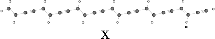
Figure 2: Oligo-di-acetylenes, with the long-axis moment of inertia aligned with the $x$-coordinate. This is the axis along which the polarisabilities are evaluated.

We carried out calculations on short all-trans oligo-di-acetylenes (ODAs), 2-ODA $\mathrm{C_{8}H_{6}}$, 4-ODA $\mathrm{C_{16}H_{10}}$, 6-ODA $\mathrm{C_{24}H_{14}}$. Optimised geometries were obtained at the density functional theory B3LYP Becke (1993); Lee et al. (1988) level in a correlation consistent Dunning double-zeta (cc-pVDZ) basis Schuchardt et al. (2007). Subsequent Hartree-Fock, DMRG, and coupled cluster (CC) calculations were carried out in a minimal STO-6G Gaussian basis Hehre et al. (1969); Schuchardt et al. (2007). We realise that this basis is too small for the quantitative calculation of polarisabilities, but it has been chosen to enable a preliminary study. Also, we note that qualitative trends in polarisabilities can be captured using rather small basis sets of split-valence quality Bredas et al. (1994). The Hartree-Fock calculations were used to determine molecular orbitals with $\sigma$ and $\pi$ character. All $\sigma$ orbitals were kept frozen in the DMRG response calculations, and the $\pi$ orbitals were localised. Calculated polarisabilities refer to the $\alpha_{xx}$ component, where the $x$-axis is aligned with the long moment of inertia axis of the molecules (see Fig. 2). The DMRG response calculations used an active space of $p_{z}$ orbitals only, corresponding to an (8e, 8orb) active space for 2-ODA, a (16e, 16orb) active space for 4-ODA, and a (24e, 24orb) active space for 6-ODA. For the analytic response DMRG calculations using $M$ states we first converged a ground-state DMRG calculation with $M$ states using the one-site algorithm, and used this as the starting point for the response calculation.

In addition to the analytic response DMRG calculations, we carried out calculations using the dynamical DMRG method for comparison. The dynamical DMRG polarisabilities were obtained by solving the linear response equation in the dynamical DMRG basis $(\omega\mathbf{1}-\mathbf{H}^{[0]})\mathbf{c}^{[1]})_{i}=\mathbf{Q}\mathbf{\mu}_{i}\mathbf{c}^{[0]}$ just as in the correction vector method, but the resulting polarisabilities were evaluated using the quadratic functional

$$G_{ij}=\mathbf{c}^{[1]{\dagger}}_{i}(\omega\mathbf{1}-\mathbf{H}^{[0]})\mathbf{c}^{[1]}_{j}+\mathbf{c}^{[0]{\dagger}}\mathbf{\mu}_{i}\mathbf{c}^{[1]}_{j}+\mathbf{c}^{[1]{\dagger}}_{j}\mathbf{\mu}_{i}\mathbf{c}^{[0]}j$$ (48)

which ensures that the obtained polarisability is quadratic in the error in $\mathbf{c}^{[1]}$ Koch and Harrison (1991); Sellers (1986), which is the hallmark of the dynamical DMRG approach. For comparison, we also computed linear-response restricted coupled cluster polarisabilities at the singles and doubles level Koch et al. (1990), both at the all electron level, and within the $p_{z}$ active space only, using the Psi3 Crawford et al. package.

We note one issue that arises with the response DMRG calculations in our initial implementation as opposed to ordinary ground-state DMRG calculations. In ground-state DMRG calculations with the one-site algorithm, we are generally able to converge the DMRG energy from sweep to sweep to very high accuracy, e.g. nanoHartrees. However, in our initial response implementation, we were not able to converge the calculated polarisabilities to similar accuracy. Typically the forward and backwards sweeps would converge to somewhat different results, and even between consecutive forwards (or backwards) sweeps, the polarisability would oscillate somewhat. This was true both for the dynamical DMRG and the analytic response DMRG calculations. The oscillation can be quite severe, particularly for small $M$ calculations and for higher frequencies that are nearer to a pole (e.g. at frequency $\omega=0.2$ a.u.) and reflects the greater sensitivity of the response calculation to the discarded states in the density matrix. In our results, we report the average polarisability of the last 4 sweeps, together with twice the standard deviation. These results are reported in table 1.

Table 1: Static and frequency dependent polarisabilities in a.u. of oligo-di-acetylenes, with 2, 4, 6 monomers (2-ODA, 4-ODA, 6-ODA). $D$ stands for dynamical DMRG, $A$ stands for analytic response theory. $\omega$ is the frequency (in a.u.), $M$ refers to the number of states in the DMRG wavefunction. The numbers in brackets do not represent intrinsic truncation error from finite $M$ but represent the numerical convergence of the DMRG sweep, since the forwards and backwards sweeps typically converge to slightly different results. The bracketed number is twice the standard deviation ($2\sigma$) in the last 4 forward and backwards sweeps. See text for further discussion.

		2-ODA		4-ODA		6-ODA
$\omega$	M	D	A	D $(2\sigma)$	A $(2\sigma)$	D $(2\sigma)$	A $(2\sigma)$
0.00	25	52.77	52.89	144.16 (0.03)	145.21 (0.04)	354.28 (17.96)	243.65 (0.06)
	50	52.89	52.89	146.07 (0.01)	145.74 (0.09)	246.04 (0.02)	245.06 (0.07)
	250	52.88	52.88	145.75 (0.01)	145.80 (0.01)	245.20 (0.00)	245.27 (0.03)
	1000	n.a.	n.a.	145.77 (0.01)	145.81 (0.00)	245.13 (0.10)	245.14 (0.02)
	LR-CCSD	53.38		148.15		249.67
0.05	25	53.98	53.96	148.46 (0.02)	149.80 (0.04)	449.82 (35.15)	252.00 (0.14)
	50	54.07	54.07	150.64 (0.01)	150.26 (0.07)	254.61 (0.02)	253.62 (0.13)
	250	54.06	54.07	150.37 (0.00)	150.39 (0.04)	253.87 (0.00)	253.92 (0.02)
	LR-CCSD	54.62		153.19		259.40
0.10	25	57.83	57.57	163.62 (0.03)	165.42 (0.13)	462.00 (22.55)	282.05 (0.25)
	50	57.99	57.99	166.46 (0.02)	166.11 (0.05)	284.81 (0.03)	283.96 (0.22)
	250	57.99	58.00	166.19 (0.00)	166.23 (0.02)	284.30 (0.00)	284.26 (0.21)
	LR-CCSD	58.72		170.76		294.16
0.15	25	65.85	64.97	195.14 (0.07)	201.06 (0.17)	557.18 (114.72)	353.66 (0.57)
	50	66.07	66.06	202.51 (0.03)	202.24 (0.09)	357.02 (0.05)	356.37 (0.20)
	250	66.05	66.08	202.45 (0.00)	202.49 (0.04)	357.26 (0.00)	357.10 (0.10)
	LR-CCSD	67.22		212.20		381.68
0.20	25	82.03	79.89	279.06 (0.35)	294.06 (0.89)	520.61 (84.68)	564.50 (1.38)
	50	82.57	82.54	296.86 (0.62)	295.83 (1.67)	564.25 (16.84)	566.94 (0.89)
	250	82.56	82.60	296.71 (0.55)	296.44 (0.06)	571.44 (0.71)	571.63 (1.73)
	LR-CCSD	84.83		328.71		682.10

From table 1 we make the following observations about the relative performance of the analytic DMRG response method relative to the dynamical DMRG method that has been commonly used. For small $M$ (e.g. $M$=25) the analytic DMRG response method is clearly superior. Whereas the dynamical DMRG method produces poor polarisabilities for $M$=25, in error by more than 50% in some cases, the analytic DMRG polarisabilities are quite reasonable at $M$=25 and typically in error by less than 1%. This is consistent with our discussion in section III.2 where we argue the the dynamical DMRG method suffers from using the same set of DMRG basis states to represent both the zeroth order DMRG vector as well as the response and perturbation vectors. Thus, for small $M$ there simply are not enough DMRG states to yield a meaningful result in the dynamical DMRG. Both methods converge as $M$ increases. For the most accurate calculations ($M$=250), although both methods perform well, the dynamical DMRG polarisabilities appear slightly better than the analytic DMRG polarisabilities. However, this appears to be related to the instabilities in the convergence of the analytic DMRG response sweeps; whereas the oscillations in the dynamical DMRG sweeps vanish for larger $M$, they still remain for the analytic DMRG sweeps. From the $2\sigma$ values, we see that currently we can only conclude that the analytic and dynamical DMRG response methods are comparable for larger $M$.

Observing the trends in the polarisabilities, we see that the polarisabilities increase as the applied frequency increases which is what one would expect since we are approaching the first excitonic ${}^{1}B_{u}$ pole. We are not able to converge our response calculations very close to a pole because of the large norm in $\mathbf{c}^{[1]}$. The standard solution to this is to include a small imaginary broadening in $\omega$. However, a straightforward incorporation of broadening leads to complex operators in the analytic theory which we have not yet implemented.

It is often the case that one wishes to determine an entire spectrum, i.e. some response property for a very large range of $\omega$. While in the dynamical DMRG this is usually performed by scanning through $\omega$ (with some small imaginary component) and performing a response calculation for each frequency, it may be more appropriate in the analytic response approach to adopt a different strategy. The coupled-perturbed response equations may be viewed as a linear eigenvalue problem for the excitation energies (i.e. poles) and may be solved in this way, in the same way that the time-dependent Hartree-Fock or time-dependent density functional equations are solved as an eigenvalue problem to obtain excitation energies. Once a sufficient number of poles are obtained, the spectrum can then be reconstructed analytically.

Comparing the DMRG polarisabilities and the coupled cluster polarisabilities, we see that the coupled cluster polarisabilities are generally quite good even at the singles and doubles level. (They appear to consistently overestimate the polarisability by only a few percent). This is not surprising since by virtue of the one-electron nature of the dipole operator, the linear polarisability only samples states with single-excitation character relative to the ground-state. Such excited states are well captured by CCSD theory. However, earlier studies indicate that the overall spectrum in conjugated systems (including e.g. doubly excited and triplet excited states) is poorly reproduced by coupled cluster theory Dorando et al. (2007), and so we would expect much larger discrepancies between the CC and DMRG description of third-order non-linear optical response.

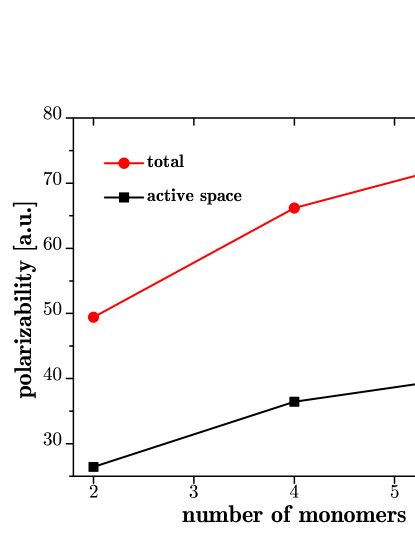
Figure 3: Scaling of total and active space polarisabilities per monomer.

In Fig. 3 we plot the static active space and total polarisabilities ($\omega=0$) per monomer calculated using the analytic DMRG response theory as a function of the number of di-acetylene monomers in the calculation. The total polarisability for the DMRG calculations is obtained using the core-correction from the linear-response coupled cluster calculations i.e.

$$\alpha^{\text{tot}}_{\text{DMRG}}=\alpha^{\text{tot}}_{CC}-\alpha^{\text{act}}_{CC}+\alpha^{\text{act}}_{DMRG}$$ (49)

We see a slow saturation of the polarisability per monomer as a function of the chain length, although the polarisability is not yet fully saturated at the 6-ODA level. While larger basis set calculations and calculations on longer chains are necessary to obtain a definitive conclusion, we note that our results are consistent with early semi-empirical calculations which indicate an onset of saturation between 2-ODA and 3-ODA Kirtman (1989).

VI Conclusions

In the current work we have described an analytic approach to the calculation of response quantities in the density matrix renormalisation group. The analytic response method is familiar from other electronic structure theories but has not so far been developed within the density matrix renormalization group. The analytic response implementation does not change the computational cost of the ground-state DMRG calculation by more than a constant factor. Compared to the popular dynamical density matrix renormalisation group approach we find that the analytic response method produces considerably more accurate response quantities when using a small number of DMRG states, without any greater computational cost. While it is simpler within the dynamical DMRG to implement higher-order response properties and complex frequencies, based on our investigations, the improved accuracy of the analytic response approach may justify the additional implementation effort. In future work, we will explore both higher-order response quantities and determination of complete spectra using the analytic DMRG response approach.

VII Acknowledgements

Support is acknowledged from the Cornell Center for Materials Research, the National Science Foundation through CHE-0645380 and the Department of Energy, Office of Science through Award No. DE-FG02-07ER46432.

References

- White (1992) S. R. White, Phys. Rev. Lett. 69, 2863 (1992).
- Schollwöck (2005) U. Schollwöck, Rev. Mod. Phys. 77, 259 (2005).
- White and Martin (1999) S. R. White and R. L. Martin, J. Chem. Phys. 110, 4127 (1999).
- Chan and Head-Gordon (2002) G. K.-L. Chan and M. Head-Gordon, J. Chem. Phys. 116, 4462 (2002).
- Ghosh et al. (2008) D. Ghosh, J. Hachmann, T. Yanai, and G. K.-L. Chan, J. Chem. Phys. 128, 144117 (2008).
- Marti et al. (2008) K. H. Marti, I. M. Ondik, G. Moritz, and M. Reiher, J. Chem. Phys. 128, 014104 (2008).
- Chan et al. (2004) G. K.-L. Chan, M. Kállay, and J. Gauss, J. Chem. Phys. 121, 6110 (2004).
- Kurashige and Yanai (2008) Y. Kurashige and T. Yanai, J. Chem. Phys. (2008), submitted.
- Zgid and Nooijen (2008a) D. Zgid and M. Nooijen, J. Chem. Phys. 128, 144116 (2008a).
- Hachmann et al. (2007) J. Hachmann, J. J. Dorando, M. Avilés, and G. K.-L. Chan, J. Chem. Phys. 127, 134309 (2007).
- Kotliar et al. (2006) G. Kotliar, Y. S. Savrasov, K. Haule, V. S. Oudovenko, O. Parcollet, and C. A. Marianetti, Rev. Mod. Phys. 78, 865 (2006).
- McWeeny and Sutcliffe (1969) R. McWeeny and B. T. Sutcliffe, Methods of Molecular Quantum Mechanics (Academic, New York, 1969).
- Jamorski et al. (1996) C. Jamorski, M. E. Casida, and D. R. Salahub, J. Chem. Phys. 104, 5134 (1996).
- Koch et al. (1990) H. Koch, H. J. A. Jensen, P. Jørgensen, and T. Helgaker, J. Chem. Phys. 93, 3345 (1990).
- Olsen and Jørgensen (1985) J. Olsen and P. Jørgensen, J. Chem. Phys. 82, 3235 (1985).
- Kobayashi et al. (1999) T. Kobayashi, K. Sasagane, F. Aiga, and K. Yamaguchi, J. Chem. Phys. 110, 11720 (1999).
- Olsen and Jørgensen (1995) J. Olsen and P. Jørgensen (1995).
- Rice and Handy (1991) J. E. Rice and N. C. Handy, J. Chem. Phys. 94, 4959 (1991).
- Sasagane et al. (1993) K. Sasagane, F. Aiga, and R. Itoh, J. Chem. Phys. 99, 3738 (1993).
- Hallberg (1995) K. A. Hallberg, Phys. Rev. B 52, 9827 (1995).
- S. Ramasesha et al. (1996) S. S. Ramasesha, S. K. Pati, H. R. Krishnamurthy, Z. Shuai, and J. L. Brédas, Phys. Rev. B 54, 7598 (1996).
- Kühner and White (1999) T. D. Kühner and S. R. White, Phys. Rev. B 60, 335 (1999).
- Jeckelmann (2002) E. Jeckelmann, Phys. Rev. B 66, 45114 (2002).
- White and Affleck (2008) S. R. White and I. Affleck, Phys. Rev. B 77, 134437 (2008).
- Jeckelmann (2008) E. Jeckelmann (2008), cond-mat.str-el/0808.2620.
- Rommer and Östlund (1997) S. Rommer and S. Östlund, Phys. Rev. B 55, 2164 (1997).
- Zgid and Nooijen (2008b) D. Zgid and M. Nooijen, J. Chem. Phys. 128, 144115 (2008b).
- S.R.White (2005) S.R.White, Phys. Rev. B. 72, 180403 (2005).
- Chan (2008) G. K.-L. Chan, Phys. Chem. Chem. Phys. 10, 3454 (2008).
- Ueda et al. (2006) K. Ueda, C. Jin, N. Shibata, Y. Hieida, and T. Nishino (2006), cond-mat.stat-mech/0612480.
- Bredas et al. (1994) J. L. Bredas, C. Adant, P. Tackx, A. Persoons, and B. M. Pierce, Chem. Rev. 94, 243 (1994).
- Becke (1993) A. D. Becke, J.Chem.Phys. 98, 5648 (1993).
- Lee et al. (1988) C. Lee, W. Yang, and R. Parr, Phys. Rev. B 37, 785 (1988).
- Schuchardt et al. (2007) K. L. Schuchardt, B. T. Didier, T. Elsethagen, L. Sun, V. Gurumoorthi, J. Chase, J. Li, and T. L. Windus, J. Chem. Inf. Model. 47, 1045 (2007).
- Hehre et al. (1969) W. J. Hehre, R. F. Stewart, and J. A. Pople, J. Chem. Phys. 51, 2657 (1969).
- Koch and Harrison (1991) H. Koch and R. J. Harrison, J. Chem. Phys. 95, 7479 (1991).
- Sellers (1986) H. Sellers, Int. J. Quantum Chem. 30, 433 (1986).
- (38) T. D. Crawford, C. D. Sherrill, E. F. Valeev, J. T. Fermann, R. A. King, M. L. Leininger, S. T. Brown, C. L. Janssen, E. T. Seidl, J. P. Kenny, et al., Psi 3.2 (2003), see www.psicode.org.
- Dorando et al. (2007) J. J. Dorando, J. Hachmann, and G. K.-L. Chan, J. Chem. Phys. 127, 084109 (2007).
- Kirtman (1989) B. Kirtman, Int. J. Quantum Chem. 36 (1989).