Parametric characterisation of a chaotic attractor using two scale Cantor measure

Abstract

A chaotic attractor is usually characterised by its multifractal spectrum which gives a geometric measure of its complexity. Here we present a characterisation using a minimal set of independant parameters which are uniquely determined by the underlying process that generates the attractor. The method maps the $f(\alpha)$ spectrum of a chaotic attractor onto that of a general two scale Cantor measure. We show that the mapping can be done for a large number of chaotic systems. In order to implement this procedure, we also propose a generalisation of the standard equations for two scale Cantor set in one dimension to that in higher dimensions. Another interesting result we have obtained both theoretically and numerically is that, the $f(\alpha)$ characterisation gives information only upto two scales, even when the underlying process generating the multifractal involves more than two scales.

I INTRODUCTION

The existence of a multifractal measure for any system most often indicates an underlying process generating it, be it multiplicative or dynamic. In the context of chaotic attractors arising from dynamical systems, their multifractal measure result from a time ordered process, which may be an iterative scheme or a continuous flow eck . The description of the invariant measures in terms of $D_{q}$ hen or $f(\alpha)$ hal3 , however, provides only a characterisation of their geometric complexity. Feigenbaum et.al fei ; feig and Amritkar and Gupte gup have shown that it is also possible to get the dynamical information in some specific cases by inverting the information contained in a multifractal measure using a thermodynamic formalism.

In this paper, we seek to get a characterisation of a chaotic attractor in terms of the underlying process that generates it. It appears that the process of generation of a multifractal chaotic attractor is similar to that of a typical Cantor set (where measure reduces after each step), with the dissipation in the system playing a major role. We show this specifically below using the example of Cat map which is area preserving. But a key difference is that, for chaotic attractors, the nature of this reduction is governed by the dynamics of the system. This implies that if the $D_{q}$ and $f(\alpha)$ curves of a chaotic attractor are mapped onto that of a model multiplicative process, one can derive information about the underlying process that generates the strange attractor, provided the mapping is correct. Here we try to implement this idea using an algorithmic scheme and show that this gives a set of parameters that can be used to characterise a given attractor.

A similar idea to extract the underlying multiplicative process from a multifractal has been applied earlier by Chhabra et.al chh1 . In order to make this inversion process successful, one needs to take into account two aspects, namely, the type of process chh1 (whether L process, P process or LP process) and the number of scales involved (whether two scale or multi scale). Chhabra et.al chh1 have shown that different multiplicative processes with only three independant parameters produce good fits to many of the observed $D_{q}$ curves. Thus the extraction of underlying multiplicative process, based solely on the information of $D_{q}$ curve, is nonunique and additional thermodynamic information is needed for the inversion process.

But the problem that we address here is slightly different. In our case, the model multiplicative process is fixed as a general two scale Cantor set which is the simplest nontrivial process giving rise to a multifractal measure. We then scan the whole set of parameters possible for this process (which include the L process, P process and LP process) and choose the statistically best fit $D_{q}$ curve to the $D_{q}$ spectrum computed for the attractor from the time series, which is then used to compute the final $f(\alpha)$ spectrum. In this way, the $f(\alpha)$ spectrum of a chaotic attractor gets mapped onto that of a general two scale Cantor set. We show that the mapping can be done for a large number of standard chaotic attractors. The resulting parameters can be considered to be unique to the underlying process that generates the attractor, upto an ambiguity regarding the number of scales involved.

The success of this procedure also implies that the $D_{q}$ and $f(\alpha)$ spectrum of a multiplicative process involving more than two scales also can be mapped onto that of a two scale Cantor set. We prove this theoretically as well as numerically in Sec.IV, by taking Cantor sets with more than two scales. This, in turn, suggests that though the $f(\alpha)$ spectrum has contributions from all the scales involved in the generation of a multifractal, the information contained in an $f(\alpha)$ spectrum is limited only upto two scales. In other words, given an $f(\alpha)$ spectrum, one can retrieve only the equivalent two scales which are different from the actual scales. Thus, while Chhabra et.al chh1 argues that additional information is needed to extract the underlying multiplicative process, our result indicate that the $f(\alpha)$ formalism itself is unable to extract more than two scales.

The motivation for using a Cantor set to characterise the multifractal structure of a chaotic attractor comes from the fact that some well known chaotic attractors are believed to have underlying Cantor set structure. For example, it has been shown spa that in the $x-y$ plane corresponding to $z=(r-1)$ of the Lorenz attractor, a transverse cut gives a multi fractal with Cantor set structure. Even the chaotic attractor resulting from the experimental Rayleigh-Bernard convection holds a support whose transverse structure is a Cantor set jen . These Cantor sets are known to be characteristic of the underlying dynamics that generate the attractor.

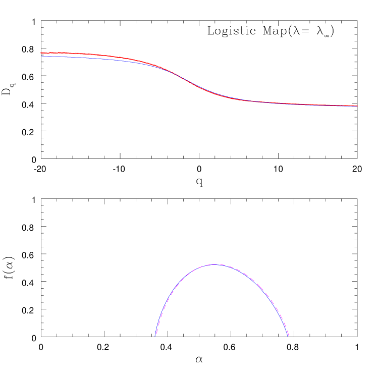
Figure 1: The upper panel shows the $D_{q}$ values (points) and its best fit curve of the strange attractor at the period doubling accumulation point of the logistic map, computed from a time series with 30000 data points. The lower panel shows the $f(\alpha)$ spectrum computed from the best fit curve (dashed line) along with the theoretically predicted curve (continuous line). The agreement between the two is evident.

A more general arguement to support the above statement is by using the concept of Kolmogorov entropy. Kolmogorov entropy can be obtained by a successively fine partition of the attractor in a hierarchical fashion. Going from one partition to the next gives one set of scales as shown in gup . These can be treated as scales of higher dimensional Cantor sets. In general, there can be several scales. But the $f(\alpha)$ curve appears to be determined by only two scales.

In order to implement our idea, the first step is to compute the $D_{q}$ spectrum of the chaotic attractor from its time series. This is done by the standard delay embedding technique gra2 , but by extending the nonsubjective scheme recently proposed by us kph for computing $D_{2}$. The $D_{q}$ spectrum is then fitted by a smooth $D_{q}$ curve obtained by inverse Legendre transformation equations atm ; gra1 of the $f(\alpha)$ curve for a general two scale Cantor set. The statistically best fit curve is chosen by changing the parameters of the fit from which, the $f(\alpha)$ curve for the time series is evaluated along with a set of independant parameters characteristic of the Cantor set. This procedure also gives a couple of other interesting results. For example, we are able to propose a generalisation of the standard equations of two scale Cantor set for higher dimensions. Moreover, we explicitely derive the equations for $D_{q}$ and $f(\alpha)$ spectrum of a three scale Cantor set and show that they can be exactly mapped onto that of a two scale Cantor set.

Our paper is organised as follows: The details of our computational scheme are presented in Sec.II and it is tested using time series from the logistic map and different Cantor sets with known parameters in Sec.III. In Sec.IV, the $f(\alpha)$ spectrum of Cantor sets with more than two scales is considered both theoretically and numerically. Sec.V is concerned with the application of the scheme to standard chaotic attractors in higher dimensions. The conclusions are drawn in Sec.VI.

II NUMERICAL SCHEME

As the first step, the spectrum of generalised dimensions $D_{q}$ are computed from the time series using the delay embedding technique gra2 . For a given embedding dimension $M$, the $D_{q}$ spectrum are given by the standard equation

$$D_{q}\equiv\frac{1}{q-1}\;\lim_{R\rightarrow 0}\frac{\log\;C_{q}(R)}{\log\;R}$$ (1)

where $C_{q}(R)$ represents the generalised correlation sum. In practical considerations, $D_{q}$ is computed by taking the slope of $\log C_{q}(R)$ versus $\log R$ over a scaling region. In our scheme, the scaling region is computed algorithmically kph for each $D_{q}$ using conditions for $R_{min}$ and $R_{max}$ and the spectrum of $D_{q}$ for $q$ in the range $[-20,20]$ is evaluated with an error bar.

Assuming that the corresponding $f(\alpha)$ curve is a smooth convex function, we seek to represent it using the standard equations hal3 ; amr of $\alpha$ and $f(\alpha)$ for the general two scale Cantor set

$$\alpha={{r\log p_{1}+(1-r)\log p_{2}}\over{r\log l_{1}+(1-r)\log l_{2}}}$$ (2)

$$f={{r\log r+(1-r)\log(1-r)}\over{r\log l_{1}+(1-r)\log l_{2}}}$$ (3)

where $l_{1}$ and $l_{2}$ are the rescaling parameters and $p_{1}$ and $p_{2}$ are the probability measures with $p_{2}=(1-p_{1})$. Thus there are three independent parameters which are characteristic of the multiplicative process generating a given $f(\alpha)$ curve. Here $r$ is a variable in the range $[0,1]$, with $r\rightarrow 0$ corresponding to one extreme of scaling and $r\rightarrow 1$ corresponding to the other extreme. Taking ${{\log p_{2}}/{\log l_{2}}}>{{\log p_{1}}/{\log l_{1}}}$, as $r\rightarrow 0$, we get

$$\alpha\rightarrow\alpha_{max}\equiv{{\log p_{2}}\over{\log l_{2}}}$$ (4)

and as $r\rightarrow 1$

$$\alpha\rightarrow\alpha_{min}\equiv{{\log p_{1}}\over{\log l_{1}}}$$ (5)

By inverting Eqs. (2) and  (3) and using the standard Legendre transformation equations atm ; gra1 connecting $\alpha$ and $f(\alpha)$ with $q$ and $D_{q}$, we get

$$q={d\over{d\alpha}}f(\alpha)$$ (6)

$$D_{q}={{{\alpha q}-{f(\alpha)}}\over{(q-1)}}$$ (7)

Changing the variable $\eta=1/r$,  (2) and  (3) reduce to

$$\alpha={{\log p_{1}+(\eta-1)\log p_{2}}\over{\log l_{1}+(\eta-1)\log l_{2}}}$$ (8)

$$f={{(\eta-1)\log(\eta-1)-{\eta\log\eta}}\over{\log l_{1}+(\eta-1)\log l_{2}}}$$ (9)

Differentiating  (8) and  (9) with respect to $\eta$ and combining

$${{df}\over{d\alpha}}={{(\log l_{1}(\log(\eta-1)-\log\eta)+\log l_{2}\log\eta)}\over{(\log l_{1}\log p_{2}-\log l_{2}\log p_{1})}}$$ (10)

Using eq. (6) and changing back to variable $r$

$$q={{df}\over{d\alpha}}={{\log l_{1}\log(1-r)-\log l_{2}\log r}\over{\log l_{1}\log(1-p_{1})-\log l_{2}\log p_{1}}}$$ (11)

Eqs. (11) and  (7) give both $q$ and $D_{q}$ as functions of the three independent parameters $l_{1},l_{2}$ and $p_{1}$.

For a given set of parameters, the $D_{q}$ curve is determined by varying $r$ in the range $[0,1]$ and fitted with the computed $D_{q}$ values from the time series. The procedure is repeated by changing the values of $p_{1}$ in the range $[0,1]$ and for each $p_{1}$, scanning the values of $l_{1}$ and $l_{2}$ with the condition that both $l_{1},l_{2}<1$. A statistical $\chi^{2}$ fitting is undertaken and the best fit curve given by the $\chi^{2}$ minimum is chosen. The complete $f(\alpha)$ curve is derived from it along with the complete set of parameters $p_{1},l_{1},l_{2},\alpha_{min}$ and $\alpha_{max}$, for a particular time series.

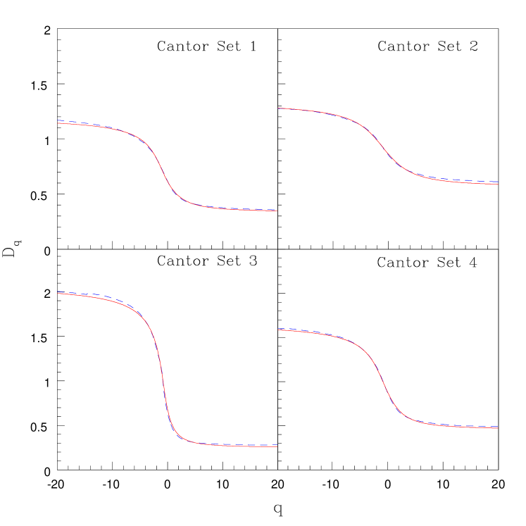
Figure 2: The $D_{q}$ values (dashed lines) of four different two scale Cantor sets computed from their time series along with the numerical fit (continuous line) in each case.

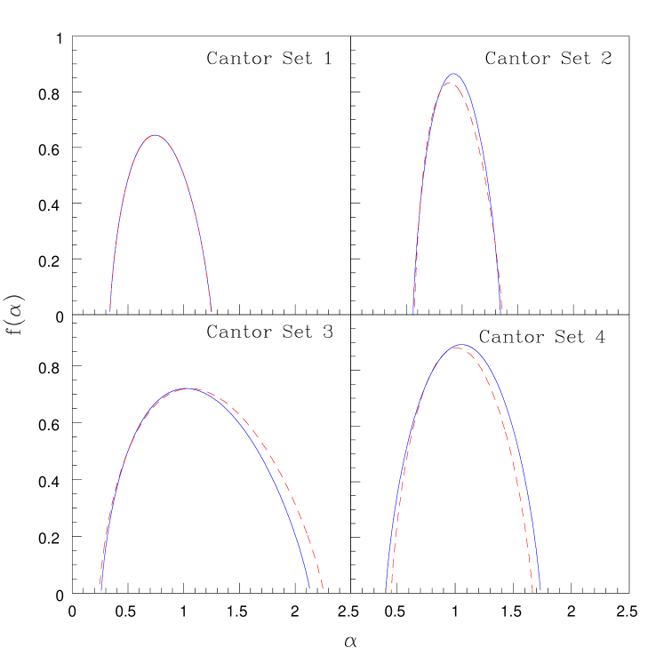
Figure 3: The $f(\alpha)$ curves for the Cantor sets shown in Fig. 2 computed from the best fit $D_{q}$ curve (dashed line) along with the theoretical curves (continuous line). The parameter values used for constructing the Cantor sets agree very well with those derived using our scheme in all the cases (see Table  1).

III TESTING THE SCHEME

In order to illustrate our scheme, we first apply it on standard multifractals where the $f(\alpha)$ curve and the associated parameters are known exactly. In all the examples discussed in this paper, $30000$ data points are used for the analysis. The first one is the time series from the logistic map at the period doubling accumulation point. The $D_{q}$ spectrum is first computed using Eq. (1) (with $M=1$), for $q$ values in the range $[-20,+20]$. The computation is done taking a step width of $\Delta q=0.1$. Choosing $p_{1}=0.5,\alpha_{min}=D_{20}$ and $\alpha_{max}=D_{-20}$ as input parameters, the $D_{q}$ curve is computed from the above set of equations and fitted with the $D_{q}$ values. The procedure is repeated by scanning $p_{1}$ in the range $[0,1]$ in steps of $0.01$. For each $p_{1}$, $\alpha_{min}$ and $\alpha_{max}$ (which in turn determine $l_{1}$ and $l_{2}$) are also varied independantly over a small range. The best fit $D_{q}$ curve is chosen as indicated by the $\chi^{2}$ minimum. Since the error in $D_{q}$ generally bulges as $q\rightarrow-20$, the error bar is also taken care of in the fitting process. The $D_{q}$ values computed from the time series and its best fit curve are shown in Fig. 1.

The complete $f(\alpha)$ spectrum for the time series is computed from the best fit $D_{q}$ curve. To make a comparison, the spectrum is also determined from Eqs. (2) and  (3) using the known values of $p_{1},l_{1}$ and $l_{2}$ for the logistic map, namely, $p_{1}=0.5$, $l_{1}=0.158(1/{\alpha_{F}^{2}})$ and $l_{2}=0.404(1/{\alpha_{F}})$ where $\alpha_{F}$ is Feigenbaum’s universal number. Both the curves are also shown in Fig. 1. The three parameters derived using our scheme are $p_{1}=0.5,l_{1}=0.146$ and $l_{2}=0.416$ which are reasonably accurate considering the finiteness of the data set.

Table 1: Comparison of the parameters used for the generation of the different Cantor sets discussed in the text with those computed by applying our numerical scheme. Close to 30000 points are used for computation in all cases.

Cantor set No.	Parameters used	Parameters computed
Cantor set 1	$p_{1}=0.60$, $l_{1}=0.22$, $l_{2}=0.48$	$p_{1}=0.58$, $l_{1}=0.21$, $l_{2}=0.49$
Cantor set 2	$p_{1}=0.42$, $l_{1}=0.22$, $l_{2}=0.67$	$p_{1}=0.45$, $l_{1}=0.24$, $l_{2}=0.67$
Cantor set 3	$p_{1}=0.66$, $l_{1}=0.18$, $l_{2}=0.62$	$p_{1}=0.69$, $l_{1}=0.19$, $l_{2}=0.64$
Cantor set 4	$p_{1}=0.72$, $l_{1}=0.44$, $l_{2}=0.48$	$p_{1}=0.66$, $l_{1}=0.39$, $l_{2}=0.52$
3Scale Cantor set	$p_{1}=0.25$, $p_{2}=0.35$, $p_{3}=0.4$
	$l_{1}=0.12$, $l_{2}=0.35$, $l_{3}=0.18$	$p_{1}=0.50$, $l_{1}=0.26$, $l_{2}=0.52$
4Scale Cantor set	$p_{1}=0.34$, $p_{2}=0.38$, $p_{3}=0.16$, $p_{4}=0.12$
	$l_{1}=0.12$, $l_{2}=0.25$, $l_{3}=0.18$, $l_{4}=0.08$	$p_{1}=0.58$, $l_{1}=0.30$, $l_{2}=0.57$

As the second example, we generate time series from four Cantor sets using four different sets of parameters as given in Table  1. Fig. 2 shows the computed $D_{q}$ values along with the best fit curves in all the four cases. Note that the fit is extremely accurate for the whole range of $q$ in all cases. The corresponding $f(\alpha)$ curves, both theoretical and computed from scheme are shown in Fig. 3. The parameter values derived from our scheme in the four cases are also given in Table  1 for comparison. It is clear that the scheme recovers the complete $f(\alpha)$ spectrum and the parameters reasonably well. In order to convince ourselves that the scheme does not produce any spurious effects, we have also applied it to a time series from a pure white noise. The $D_{q}$ versus $q$ curve for white noise should be a straight line parallel to the $q$ axis with $D_{0}=M$. The corresponding $f(\alpha)$ spectrum would be a $\delta$ function which has been verified numerically.

Figure 4: The construction of a general 3 scale Cantor set.

From the numerical computations of two scale Cantor sets, we also find the following results: While the end points of the spectrum, $\alpha_{min}$ and $\alpha_{max}$, are determined by the ratios $\log{p_{1}}/\log{l_{1}}$ and $\log{p_{2}}/\log{l_{2}}$, the peak value $D_{0}$ is determined by only the rescaling parameters $l_{1}$ and $l_{2}$. As $(l_{1}+l_{2})$ increases (that is, as the gap length decreases), $D_{0}$ also increases and $D_{0}\rightarrow 1$ as $(l_{1}+l_{2})\rightarrow 1$. In this sense, the gap length also influences the $f(\alpha)$ spectrum indirectly. We will show below that this is not true in the case of three scale Cantor set where we miss some information regarding the scales. We also find that as the difference between $\alpha_{min}$ and $\alpha_{max}$ increases (that is, as the spectrum widens), more number of data points are required, in general, to get good agreement between theoretical and numerical $f(\alpha)$ curves.

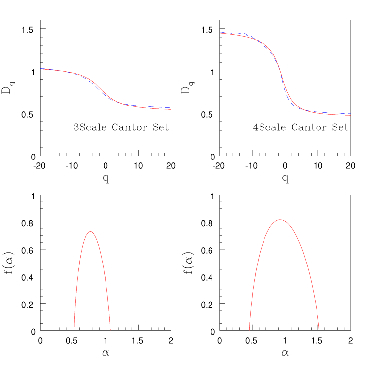
Figure 5: The $D_{q}$ and $f(\alpha)$ curves of a 3 scale and a 4 scale Cantor set computed using our scheme. The $D_{q}$ curves computed from the time series (dashed lines) are fitted with that of equivalent two scale Cantor sets (continuous lines) in both cases. The parameters used and computed by the scheme are compared in Table  1.

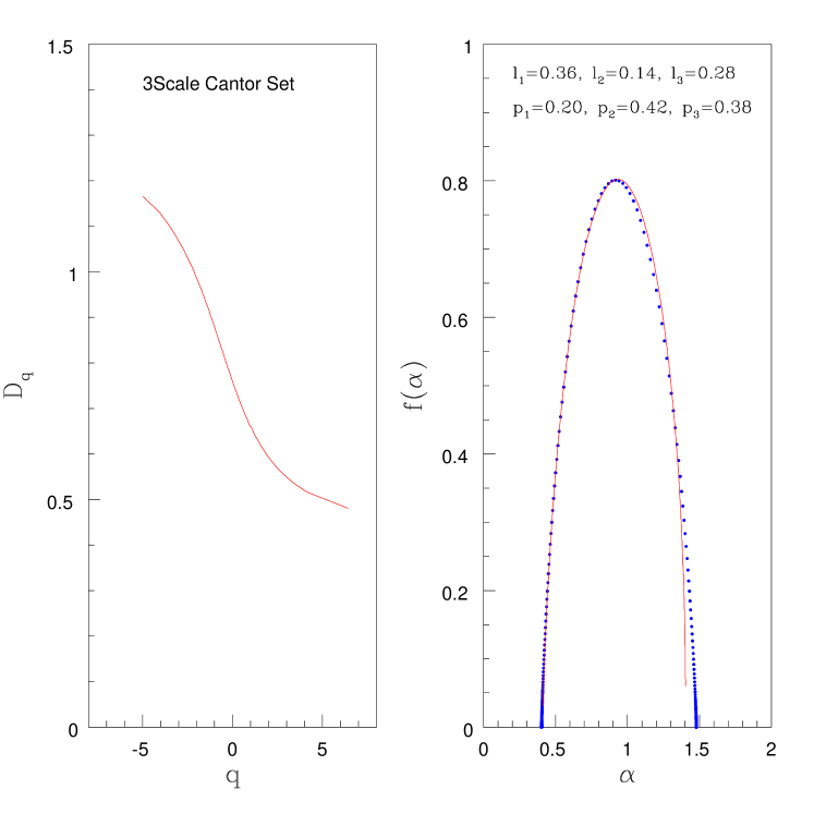
Figure 6: The left panel shows the theoretical $D_{q}$ curve of a 3 scale Cantor set with parameters shown in the figure. The right panel shows the corresponding $f(\alpha)$ curve (continuous line) calculated theoretically using Eqs.  (22) and  (24). This is superimposed on the $f(\alpha)$ spectrum (points) computed using our numerical code by fitting 2 scale Cantor set. Close to 30000 data points are used for the computations.

IV MULTI SCALE CANTOR SETS

In this section, we consider the $f(\alpha)$ spectrum of a Cantor set with more than two scales. First we show the numerical results using our scheme. For this, we first generate the time series for a general 3 scale Cantor set and compute its $D_{q}$ spectrum. The geometrical construction of a general 3 scale Cantor set is shown in Fig. 4. At every stage, an interval gets subdivided into three so that the set involves 3 rescaling parameters $l_{1}$, $l_{2}$, $l_{3}$ and 3 probability measures $p_{1}$, $p_{2}$, $p_{3}$ as shown. The numerically computed $D_{q}$ spectrum for a typical 3 scale Cantor set (with parameters given in Table  1) is shown in Fig. 5 (upper left panel). The $D_{q}$ curve can be very well fitted by a 2 scale Cantor set and the complete $f(\alpha)$ spectrum for the 3 scale Cantor set is evaluated (lower left panel). We have repeated our computations for a 4 scale Cantor set as well and the results are also shown in Fig. 5 (right panel). In both cases, the parameters used for the construction of the Cantor sets and those computed by our scheme are given in Table  1. Thus it is clear that the $f(\alpha)$ spectrum cannot pick up the full information about the various scales and probability measures. No matter how many scales are involved in the generation of the multifractal, the $f(\alpha)$ spectrum can be reproduced by an equivalent 2 scale Cantor set.

We now derive explicite expressions for $\alpha$ and $f(\alpha)$ for a 3 scale Cantor set. We follow the arguements given in Halsey et.al hal3 , Sec.II-C-4. For the 3 scale Cantor set, one can write

$$\Gamma(q,\tau,n)=\left({{p_{1}^{q}}\over{l_{1}^{\tau}}}+{{p_{2}^{q}}\over{l_{2}^{\tau}}}+{{p_{3}^{q}}\over{l_{3}^{\tau}}}\right)^{n}=1$$ (12)

Expanding

$$\Gamma(q,\tau,n)=\sum_{m_{1},m_{2}}{{n!}\over{m_{1}!m_{2}!(m-m_{1}-m_{2})!}}p_{1}^{m_{1}q}p_{2}^{m_{2}q}p_{3}^{(m-m_{1}-m_{2})q}l_{1}^{-m_{1}\tau}l_{2}^{-m_{2}\tau}l_{3}^{-(m-m_{1}-m_{2})\tau}=1$$ (13)

In the limit $n\rightarrow\infty$, the largest term contributes. Hence we have

$${{\partial\Gamma}\over{\partial m_{1}}}=0$$ (14)

$${{\partial\Gamma}\over{\partial m_{2}}}=0$$ (15)

Using the Stirling approximation and simplifying the above two conditions we get

$$-\log r+\log(1-r-s)+q\log(p_{1}/p_{3})-\tau\log(l_{1}/l_{3})=0$$ (16)

$$-\log s+\log(1-r-s)+q\log(p_{2}/p_{3})-\tau\log(l_{2}/l_{3})=0$$ (17)

where $r=m_{1}/n$ and $s=m_{2}/n$ are free parameters. Also from Eq. (13), using a similar procedure, one can show that

$$r\log r-s\log s-(1-r-s)\log(1-r-s)+q(r\log p_{1}+s\log p_{2}+(1-r-s)\log p_{3})-\tau(r\log l_{1}+s\log l_{2}+(1-r-s)\log l_{3})=0$$ (18)

Combining Eqs. (16),  (17) and  (18) and eliminating $\tau$ we get the following relations for $q$

$$q={{\log(l_{2}/l_{3})\log((1-r-s)/r)-\log(l_{1}/l_{3})\log((1-r-s)/s)}\over{\log(l_{1}/l_{3})\log(p_{2}/p_{3})-\log(l_{2}/l_{3})\log(p_{1}/p_{3})}}$$ (19)

$$q={{\log(l_{1}/l_{3})(-r\log r-s\log s-(1-r-s)\log(1-r-s))-(r\log l_{1}+s\log l_{2}+(1-r-s)\log l_{3})\log((1-r-s)/r)}\over{(r\log l_{1}+s\log l_{2}+(1-r-s)\log l_{3})\log(p_{1}/p_{3})-\log(l_{1}/l_{3})(r\log p_{1}+s\log p_{2}+(1-r-s)\log p_{3})}}$$ (20)

These two equations for $q$ can be used to obtain a relation between $r$ and $s$.

To compute the $D_{q}$ spectrum, vary $r$ from 0 to 1. For every value of $r$, the value of $s$ that satisfies the Eqs. (19) and  (20)simultaneously is computed numerically, with the condition that $0<s<(1-r)$. For every value of $r$ and $s$, $q$ and $\tau$ can be determined using Eqs. (19) and  (16), which in turn gives $D_{q}=\tau/(q-1)$.

The singularity exponent $\alpha$ is determined by the condition

$$p_{1}^{m_{1}}p_{2}^{m_{2}}p_{3}^{(m-m_{1}-m_{2})}=\left(l_{1}^{m_{1}}l_{2}^{m_{2}}l_{3}^{(m-m_{1}-m_{2})}\right)^{\alpha}$$ (21)

This gives the expression for $\alpha$

$$\alpha={{r\log p_{1}+s\log p_{2}+(1-r-s)\log p_{3}}\over{r\log l_{1}+s\log l_{2}+(1-r-s)\log l_{3}}}$$ (22)

Similarly, the density exponent $f(\alpha)$ is determined by

$$n!\left(l_{1}^{m_{1}}l_{2}^{m_{2}}l_{3}^{(m-m_{1}-m_{2})}\right)^{f(\alpha)}=m_{1}!m_{2}!(m-m_{1}-m_{2})!$$ (23)

which gives the following expression for $f(\alpha)$

$$f(\alpha)={{r\log r+s\log s+(1-r-s)\log(1-r-s)}\over{r\log l_{1}+s\log l_{2}+(1-r-s)\log l_{3}}}$$ (24)

By varying $r$ from 0 to 1, the $f(\alpha)$ spectrum for a given 3 scale Cantor set can be determined theoretically. In Fig. 6, the theoretically computed $D_{q}$ and $f(\alpha)$ spectrum for a typical 3 scale Cantor set is shown. Along with the theoretical $f(\alpha)$ curve, we also show the numerical one (points) for the same Cantor set, computed using our scheme. Thus it is evident that the $f(\alpha)$ spectrum of a 3 scale Cantor set can be mapped onto that of a 2 scale Cantor set. Also, our numerical results on 4 scale Cantor set (Fig. 5) suggests that this mapping onto 2 scale Cantor set can possibly be extended for the $f(\alpha)$ spectrum of four or more scale Cantor sets.

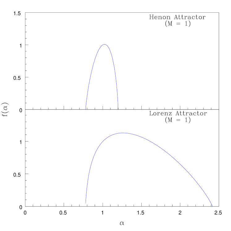
Figure 7: The multifractal spectrum of the one dimensional projection of Henon and Lorenz attractors, which show the underlying Cantor set structure. Note that the peak values of the spectrum in both cases are equal to 1.

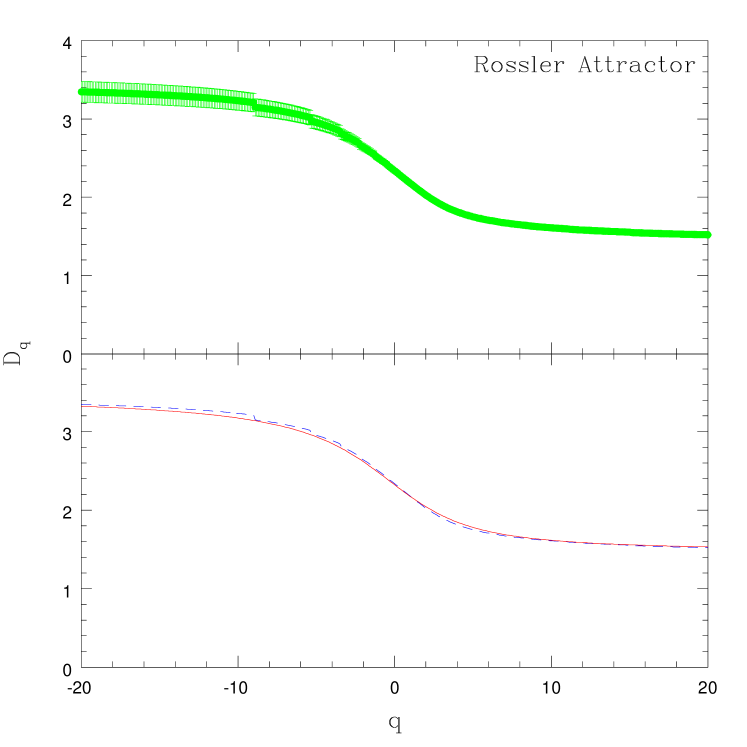
Figure 8: The upper panel gives the $D_{q}$ spectrum, with error bar, of the Rossler attractor computed from the time series. The lower panel shows the accuracy of fitting with again the $D_{q}$ values (dashed line) and its best fit curve (continuous line) computed using the scheme.

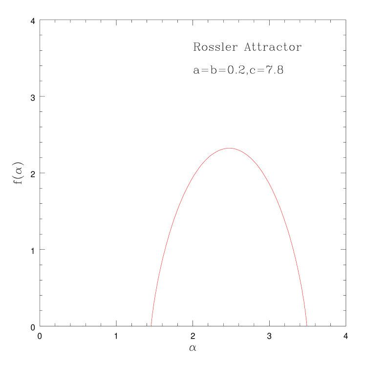
Figure 9: The $f(\alpha)$ curve of the Rossler attractor computed from the best fit $D_{q}$ curve shown in Fig. 8.

V CHARACTERISATION OF STRANGE ATTRACTORS

Evaluating the $f(\alpha)$ spectrum of one dimensional sets is straightforward. But computing the spectra of even synthetic higher dimensional attractors is a challenging task. Generally, the $f(\alpha)$ spectrum for higher dimensional chaotic attractors is calculated taking only one dimension elg ; chh3 ; wik , which characterise the transverse self similar structure on the attractor equivalent to a Cantor set. In the resulting $f(\alpha)$ spectrum, the peak value (that is, $D_{0}$) will be equal to $1$, as the higher dimensional attractor is projected into one dimension. This is shown in Fig. 7 for Henon and Lorenz attractors and the results are consistent with the earlier results.

In order to extend our scheme to higher dimensional strange attractors, their $f(\alpha)$ spectra are to be considered analogous to a two scale Cantor measure in higher dimensions. While the $f(\alpha)$ curve can be recovered using the correct embedding dimension $M$, the meaning of the parameters have to be interpreted properly. For a one dimensional Cantor set, $p_{1}$ is a probability measure while $l_{1}$ and $l_{2}$ are fractional lengths at each stage. Extending this analogy to two and three dimensions, $p_{1}$ can still be interpreted as a probability measure for the two higher dimensional scales, say $\tau_{1}$ and $\tau_{2}$. These can be considered as fractional measures corresponding to area or volume depending on the embedding dimension $M$. In other words, $p_{1}$ is a measure representing the underlying dynamics, while $\tau_{1}$ and $\tau_{2}$ correspond to geometric scaling. This gives an alternate description of the formation of a strange attractor if it is correlated to a higher dimensional analogue of the Cantor set.

As discussed in Sec.II, for the one dimensional Cantor set, $\alpha_{min}$ and $\alpha_{max}$ are given by Eqs. (4) and  (5) in terms of the parameters. For $p_{1}=p_{2}$ and $l_{1}=l_{2},\alpha_{min}=\alpha_{max}\leq 1$ and the set becomes a simple fractal with $\alpha\equiv f(\alpha)=D_{0}$, the fractal dimension. Extending this analogy to higher dimensions, we propose that Eqs. (4) and  (5) are to be modified as

$$\alpha_{max}=M{{\log p_{2}}\over{\log\tau_{2}}}$$ (25)

and

$$\alpha_{min}=M{{\log p_{1}}\over{\log\tau_{1}}}$$ (26)

As in the case of one dimensional Cantor sets, for $p_{1}=p_{2}$ and $\tau_{1}=\tau_{2}$, $\alpha_{max}=\alpha_{min}\leq M$ and the set is again a simple fractal with fractal dimension $D_{0}=\alpha\equiv f(\alpha)$. Rewriting the above equations,

$$\alpha_{max}={{\log p_{2}}\over{\log({\tau_{2}}^{1/M})}}={{\log p_{2}}\over{\log l_{2}}}$$ (27)

and

$$\alpha_{min}={{\log p_{1}}\over{\log({\tau_{1}}^{1/M})}}={{\log p_{1}}\over{\log l_{1}}}$$ (28)

Replacing $l_{1}$ and $l_{2}$ by $\tau_{1}^{1/M}$ and $\tau_{2}^{1/M}$ in Eqs. (2) and  (3), the defining equations for the two scale Cantor set in $M$ dimension can be generalised as

$$\alpha={M[{r\log p_{1}+(1-r)\log p_{2}}]\over{r\log{\tau_{1}}+(1-r)\log{\tau_{2}}}}$$ (29)

$$f={M[{r\log r+(1-r)\log(1-r)}]\over{r\log{\tau_{1}}+(1-r)\log{\tau_{2}}}}$$ (30)

Just like $l_{1}+l_{2}<1$ for one dimensional Cantor set, we expect $\tau_{1}+\tau_{2}<1$ in $M$ dimensions. This is because, the measure keeps on reducing after each time step due to dissipation and $\tau_{1}$ and $\tau_{2}$ represent the fractional reduction in the measure for the two scales. It should be noted that since, in general, different scales apply in different directions, $\tau_{1}$ and $\tau_{2}$ should be treated as some effective scales in higher dimension.

Table 2: The complete set of parameters computed using our scheme for six standard chaotic attractors. See spr , for example, for the details of the chaotic systems and the values of the parameters used.

Attractor	$\alpha_{min}$	$\alpha_{max}$	$D_{0}$	$p_{1}$	$\tau_{1}$	$\tau_{2}$
Rossler attractor
($a=b=0.2,c=7.8$)	$1.46\pm 0.02$	$3.39\pm 0.14$	$2.31\pm 0.02$	$0.65$	$0.42$	$0.41$
Lorenz attractor
($\sigma=10,r=28,b=8/3$)	$1.38\pm 0.03$	$3.71\pm 0.12$	$2.16\pm 0.04$	$0.50$	$0.22$	$0.57$
Ueda attractor
($k=0.05,A=7.5$)	$1.73\pm 0.05$	$3.78\pm 0.13$	$2.62\pm 0.06$	$0.64$	$0.46$	$0.44$
Duffing attractor
($b=0.25,A=0.4,\Omega=1$)	$1.84\pm 0.04$	$3.59\pm 0.08$	$2.78\pm 0.04$	$0.81$	$0.71$	$0.25$
Henon attractor
($a=1.4,b=0.3$)	$0.96\pm 0.02$	$2.27\pm 0.08$	$1.43\pm 0.03$	$0.50$	$0.24$	$0.54$
Tinkerbell attractor
($a=0.9,b=-0.6,c=2,d=0.5$)	$0.83\pm 0.02$	$3.43\pm 0.12$	$1.65\pm 0.03$	$0.60$	$0.29$	$0.58$

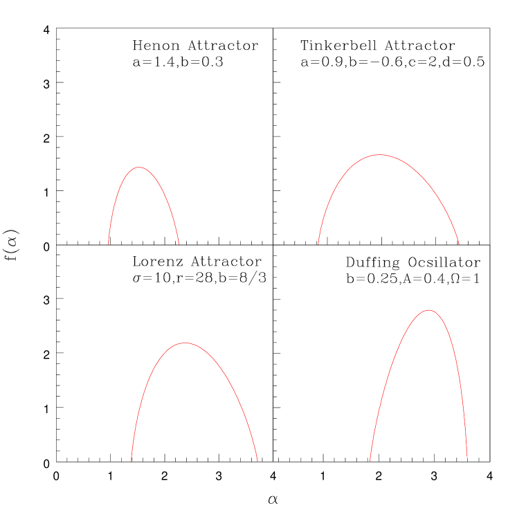
Figure 10: The multifractal spectrum of four standard chaotic attractors computed by applying our algorithmic scheme. The parameter values used for generating the time series are also shown.

Figure 11: The $D_{q}$ curve of the Cat map (left panel) computed using our scheme which is a straight line parallel to the $q$ axis just like that of a white noise. The corresponding $f(\alpha)$ curve is shown in the right panel, which is $\delta$ function with $\alpha\equiv f(\alpha)=2$.

We now check these results using the time series from a standard chaotic attractor, namely the Rossler attractor for parameter values $a=b=0.2$ and $c=7.8$ with $30000$ data points. Fig. 8 shows the $D_{q}$ spectrum computed from the time series taking $M=3$, along with the best fit curve applying our scheme. The fit is found to be very good for the whole range of $q$ values. The complete $f(\alpha)$ spectrum computed from the best fit $D_{q}$ curve is shown in Fig. 9. The scheme also calculates the three parameters as $p_{1}=0.65$, $\tau_{1}=0.42$ and $\tau_{2}=0.41$ so that $\tau_{1}+\tau_{2}=0.83<1$. Thus one can say that if the $f(\alpha)$ spectrum of the Rossler attractor is made equivalent to a two scale Cantor set in three dimension, the resulting probability measures are $0.65$ and $0.35$ and rescaling parameters $0.42$ and $0.41$. Interestingly, it appears that the Rossler attractor is generated by a P process rather than a LP process.

The scheme has also been applied to several standard chaotic attractors in two and three dimensions. The $f(\alpha)$ spectrum are shown in Fig. 10 for four of them, while the complete set of parameters for six standard chaotic attractors are given in Table  2. The error bars given for $\alpha_{max},\alpha_{min}$ and $D_{0}$ are those reflected from the computed $D_{q}$ values. In a way, the two sets of parameters given above, that is $p_{1},\tau_{1},\tau_{2}$ and $\alpha_{max},\alpha_{min},D_{0}$, can be considered as complementary to each other. While the former contain the finger prints of the underlying process that generate the strange attractor (the extent of stretching and folding and redistribution of measures at each time step), the latter characterises the geometric complexity of the attractor once it is formed. Both can be independantly used to differentiate between chaotic attractors formed from different systems or from the same system for different parameter values. The former may be more relevant in the case of chaotic attractors obtained from experimental systems.

Finally, we wish to point out that dissipation is a key factor leading to the multifractal nature of a chaotic attractor. To show this, we consider a counter example, namely, that of Cat map which is area preserving. The fixed points of the Cat map are hyperbolic, which are neither attractors nor repellers and the trajectories uniformly fill the phase space as time $t\rightarrow\infty$. Its $D_{q}$ spectrum computed from the time series is found to be a straight line as shown in Fig. 11, just like that of a white noise. The corresponding $f(\alpha)$ curve is a $\delta$ function, also shown in Fig. 11. Since $\alpha_{min}=\alpha_{max}$, a two scale fit gives the parameters as $p_{1}=0.5,\tau_{1}=0.49$ and $\tau_{2}=0.51$. Thus the Cat map attractor turns out to be a simple fractal rather than a multifractal.

VI DISCUSSION AND CONCLUSION

In this paper, we show that a chaotic attractor can be characterised using a set of three independant parameters which are specific to the underlying process generating it. The method relies on a scheme that maps the $f(\alpha)$ spectrum of a chaotic attractor onto that of a general two scale Cantor set. The scheme is first tested using one dimensional chaotic attractors and Cantor sets whose $f(\alpha)$ curves and parameters are known and subsequently applied to higher dimensional cases.

In the scheme, the $D_{q}$ spectrum of a chaotic attractor is compared with the $D_{q}$ curve computed from a model multiplicative process. Similar idea has also been used to deduce certain statistical characteristics of a system and infer features of the dynamical processes leading to the observed macroscopic parameters. One such example has been provided earlier by Meneveau and Sreenivasan sre2 in the study of energy dissipation rate in fully developed turbulent flows. By comparing the experimental $D_{q}$ data with that of a two scale Cantor measure, they have shown that the dynamics leading to the observed multifractal distributions of the energy dissipation rate can be well approximated by a single multi step process involving unequal energy distribution in the ratio $7/3$.

Usually, a multifractal is characterised only by the range of scaling involved $[\alpha_{min},\alpha_{max}]$, which roughly represents the inhomogeinity of the attractor. So the set of parameters computed here seems to give alternative way of characterising them. But we wish to emphasize that the information contained in these parameters is more subtle. For example, once these prameters are known, $\alpha_{min}$ and $\alpha_{max}$ can be determined using Eqs. (27) and  (28). Thus by evaluating $p_{1}$, $l_{1}$ and $l_{2}$, we get additional information regarding the dynamic process leading to the generation of the strange attractor. Moreover, these parameters can also give indication as to why the degree of inhomogeinity varies between different chaotic attractors. As is well known from the srudy of Cantor sets, the primary reason for the increased inhomogeinity is the wide difference between the rescaling measures $l_{1}$ and $l_{2}$. Looking at the parameter values, rescaling measures $\tau_{1}$ and $\tau_{2}$ are very close for Rossler and Ueda attractors which appear less inhomogeneous, while that for Lorenz and Duffing are widely different making them more inhomogeneous with two clear scrolls.

Another novel aspect of the scheme worth commenting is the use of two scale Cantor measures in higher dimension as analogues of chaotic attractors. Eventhough such objects are not much discussed in the literature, one can envisage them, for example, as generalisation of the well known Sierpinsky carpets in two dimension or the Menger sponge in three dimension. But a key difference between these and a chaotic attractor is that the rescaled measures are not regular in the generation of the latter. Recently, Perfect et. al per present a general theoretical framework for generating geometrical multifractal Sierpinsky carpets using a generator with variable mass fractions determined by the truncated binomial probability distribution and to compute their generalised dimensions. It turns out that the chaotic attractors are more similar to multifractals generated in higher dimensional support, such as, fractal growth patterns and since the rescaled measures are irregular, a one dimensional measure such as $l_{1}=\tau_{1}^{1/M}$ need not have any physical significance.

Finally, for a complex chaotic attractor in general, the redistribution of the measures as it evolves in time can take place in more than two scales. Thus it appears that a characterisation based on only two scales is rather approximate as we tend to lose some information regarding the other scales involved. But we have found that the $D_{q}$ and $f(\alpha)$ curves of a multi scale Cantor set can be mapped onto that of an equivalent two scale Cantor set. These two scales may be functions of the actual scales involved and may contain the missing information in an implicit way. Thus, an important outcome of the present analysis is the realisation that the dynamical information that can be retrieved from the $f(\alpha)$ spectrum is limited to only two scales. In this sense, a two scale Cantor measure can be considered as a good approximation to describe the multifractal properties of natural systems.

- (1) J. P. Eckmann and D. Ruelle, Rev. Mod. Phys. 57, 617(1985).
- (2) H. G. E. Hentschel and I. Proccacia, Physica D 8, 435(1983).
- (3) T. C. Halsey, M. H. Jensen, L. P. Kadanoff, I. Proccacia and B. I. Shraiman, Phys. Rev. A 33, 1141(1986).
- (4) M. J. Feigenbaum, M. H. Jensen and I. Proccacia, Phys. Rev. Lett. 57, 1503(1986).
- (5) M. J. Feigenbaum, J. Stat. Phys. 46, 919(1987); 925(1987).
- (6) R. E. Amritkar and N. Gupte, Phys. Rev. Lett. 60, 245(1988).
- (7) A. B. Chhabra, R. V. Jensen and K. R. Sreenivasan, Phys. Rev. A 40, 4593(1989).
- (8) C. Sparrow, The Lorenz Equations: Bifurcations, Chaos and Strange Attractors, (Springer, New York, 1982).
- (9) M. H. Jensen, L. P. Kadanoff, A. Lichaber, I. Proccacia and J. Stavans, Phys. Rev. Lett. 55, 2798(1985).
- (10) P. Grassberger and I. Proccacia, Physica D 9, 189(1983).
- (11) K. P. Harikrishnan, R. Misra, G. Ambika and A. K. Kembhavi, Physica D 215, 137(2006).
- (12) H. Atmanspacher, H. Scheingraber and G. Wiedenmann, Phys. Rev. A 40, 3954(1984).
- (13) P. Grassberger, R. Badii and A. Politi, J. Stat. Phys. 51, 135(1988).
- (14) R. E. Amritkar, A. D. Gangal and N. Gupte, Phys. Rev. A 36, 2850(1987).
- (15) S. Gratrix and J. N. Elgis, Phys. Rev. Lett. 92, 014101(2004).
- (16) A. B. Chhabra, C. Meneveau, R. V. Jensen and K. R. Sreenivasan, Phys. Rev. A 40, 5284(1989).
- (17) K. O. Wiklund and J. N. Elgin, Phys. Rev. E 54, 1111(1996).
- (18) J. C. Sprott, Chaos and Time Series Analysis, (Oxford University Press, New York, 2003).
- (19) C. Meneveau and K. R. Sreenivasan, Phys. Rev. Lett. 59, 1424(1987).
- (20) E. Perfect, R. W. Gentry, M. C. Sukop and J. E. Lawson, Geoderma 134, 240(2006).