Statistical Performance Analysis of MDL Source Enumeration in Array Processing

Abstract

In this correspondence, we focus on the performance analysis of the widely-used minimum description length (MDL) source enumeration technique in array processing. Unfortunately, available theoretical analysis exhibit deviation from the simulation results. We present an accurate and insightful performance analysis for the probability of missed detection. We also show that the statistical performance of the MDL is approximately the same under both deterministic and stochastic signal models. Simulation results show the superiority of the proposed analysis over available results.

EDICS Category: SAM-PERF, SAM-SDET

I Introduction and Preliminaries

MDL [1], is one of the most successful methods for determining the number of present signals in array processing and channel order detection [2]. MDL is a low complexity information theoretic criteria which does not need any subjective threshold setting usual in detection theoretic criteria. Other statistical properties, specially its asymptotic consistency [1], makes it a favorable choice for source enumeration. Unfortunately, only few approximate finite-sample performance analysis are available on the MDL method [3, 4, 5, 6, 8, 7]. In [3], a simple asymptotic statistical model for the eigenvalues of the sample correlation matrix was used. Unfortunately, the theoretical results showed persistent bias from the simulation results [4].

The next work [5], gives a computational approach for calculation of the probability of false alarm $p_{fa}$. In calculating the probability of missed detection $p_{m}$, the same inaccurate statistical model is used as in [3]. In [6], instead of exact performance estimation, theoretical bounds for performance were presented. A qualitative performance evaluation in terms of gap between noise and signal eigenvalues and also the dispersion of each group is given in [7]. In a recent work [8], a significantly different approach was used. Our simulation results show improved results of [8] in comparison with [3]. The performance analysis was generalized to the non-Gaussian signals while it was shown that the results reduce to the results of [5, 6] in Gaussian signals. We will show that the same modelling errors have degraded the analysis in [8] as in [3, 4, 5, 6].

In this correspondence, we use an approach very similar to [3, 4, 5] to estimate $p_{m}$, including in the analysis the finite sample $\mathcal{O}(n^{-1})$ biases of the eigenvalues. The noise subspace eigenvalue spread is taken into account which prevents the signal subspace eigenvalues to approach $\sigma^{2}$, the noise variance. The bias of the noise power estimator in MDL is calculated to get excellent match between theoretical and simulation results. We will not calculate $p_{fa}$ which is negligible.

In the previous works, only the case of stochastic signal has been considered. Here, we use a perturbation analysis to calculate biases and variances of the eigenvalues under deterministic signal, too. Using these results, we show that the performance of source enumeration methods are approximately the same in both stochastic and deterministic signal models. This is a natural complementary result for the known fact that the performance of the DOA (Direction of Arrival) estimation methods in array processing is the same under stochastic and deterministic signal models [9].

From a sensor array of $L$ elements, $n$ observations $\boldsymbol{x}_{i}\in\mathbb{C}^{L\times 1},i=1,\ldots,n$ is made, which is a linear transformation of $d<L$ source signals $\boldsymbol{s}_{i}\in\mathbb{C}^{\,d\times 1}$, plus noise $\boldsymbol{\nu}_{i}\in\mathbb{C}^{L\!\times 1}$

$$\boldsymbol{x}_{i}=\boldsymbol{A}(\boldsymbol{\theta})\boldsymbol{s}_{i}+\boldsymbol{\nu}_{i}$$ (1)

where $\boldsymbol{A}\in\mathbb{C}^{L\!\times d}$, the steering matrix, is composed of $d$ linearly independent column vectors of array response $\boldsymbol{a}(\theta_{k}),k=1,\ldots,d$. Let $\boldsymbol{X}\triangleq[\boldsymbol{x}_{1},\ldots,\boldsymbol{x}_{n}]$ and $\boldsymbol{S}$ and $\boldsymbol{V}$ be defined in the same way. Signal and noise are assumed to be iid and uncorrelated random variables. A compact form for the model will be

$$\boldsymbol{X}=\boldsymbol{A}(\boldsymbol{\theta})\boldsymbol{S}+\boldsymbol{V}.$$ (2)

Noise is assumed to be circular Gaussian. Signal can be modelled either as a zero-mean circular Gaussian random sequence or an unknown deterministic sequence. The distribution of $\boldsymbol{x}$ will be as $\mathcal{N}(\boldsymbol{0},\boldsymbol{APA}^{\textrm{H}}+\sigma^{2}\boldsymbol{I})$ where $\boldsymbol{P}=E(\boldsymbol{ss}^{\textrm{H}})$ in the stochastic signal model, and as $\mathcal{N}(\boldsymbol{As}\,,\sigma^{2}\boldsymbol{I})$ in the deterministic signal model.

To estimate the number of present signals $d$, eigenvalues of the correlation matrix $\boldsymbol{R}=n^{-1}E(\boldsymbol{XX}^{\textrm{H}})$ are used. Note that $\boldsymbol{R}_{det}=n^{-1}\boldsymbol{ASS\,}^{\textrm{H}}\!\boldsymbol{A}^{\textrm{H}}+\sigma^{2}\boldsymbol{I}$ and $\boldsymbol{R}_{sto}=\boldsymbol{APA}^{\textrm{H}}+\sigma^{2}\boldsymbol{I}$. The eigendecomposition of the correlation matrix is

$$\boldsymbol{Rv}_{i}=\lambda_{i}\boldsymbol{v}_{i}$$ (3)

and we have $\lambda_{1}>\cdots>\lambda_{d}>\lambda_{d+1}=\cdots=\lambda_{L}=\sigma^{2}$. Source enumeration methods are based on a spherity test on the sample correlation matrix defined as

$$\hat{\boldsymbol{R}}=\frac{1}{n}\sum_{i\,=1}^{n}\boldsymbol{x}_{i}\boldsymbol{x}_{i}^{\textrm{H}}.$$ (4)

Eigendecomposition of $\hat{\boldsymbol{R}}$ is defined as $\boldsymbol{\hat{R}w}_{i}=l_{i}\boldsymbol{w}_{i}$ in which $l_{1}>l_{2}>\cdots>l_{L}$. The MDL estimator of $d$ is the minimizer of the following criterion

$$\Lambda(d,L,n)=n(L-d\,)\log\bigg{(}\frac{a_{d}}{g_{d}}\bigg{)}+\frac{1}{2}\,d(2L-d)\log(n)$$ (5)

where

$$a_{d}\triangleq\frac{1}{L-d}\sum_{i=d+1}^{L}l_{i}$$ (6)

$$g_{d}\triangleq\prod_{i=d+1}^{L}l_{i}^{1/(L-d)}$$ (7)

The first term in (5) is the generalized likelihood ratio for the test of spherity and the second term is a penalty function preventing over-modelling.

II Statistical Properties of Eigenvalues

II-A Signal Eigenvalues

First of all, we derive a result useful for statistical characterization of the signal eigenvalues in the deterministic signal model. Let $\boldsymbol{x}_{i}\in\mathbb{C}^{\,L\!\times 1}\,,\,i=1,\ldots,n$ be i.i.d. observations and $\boldsymbol{x}_{i}\sim\mathcal{N}(\boldsymbol{0},\boldsymbol{\Sigma}\,)$. Note that $\textrm{vec}\,(\boldsymbol{X})\sim\mathcal{N}(\boldsymbol{0}\,,\boldsymbol{I}_{n}\otimes\boldsymbol{\Sigma}\,)$, where $\otimes$ is the Kronecker product and $\textrm{vec}(\boldsymbol{X})$ is the vectorizing operator stacking columns of $\boldsymbol{x}$ in a single column vector. Let $\boldsymbol{\alpha},\boldsymbol{\beta},\boldsymbol{\gamma},\boldsymbol{\zeta}\in\mathbb{C}^{L\!\times 1}$ be constant vectors. The Brillinger result states that [10, p. 114]:

$$\textrm{Cov}(\boldsymbol{\alpha}^{\textrm{H}}\hat{\boldsymbol{R}}\,\boldsymbol{\beta}\,,\boldsymbol{\gamma}^{\textrm{H}}\hat{\boldsymbol{R}}\,\boldsymbol{\zeta})=n^{-1}(\boldsymbol{\alpha}^{\textrm{H}}\boldsymbol{\Sigma}\,\boldsymbol{\gamma})(\boldsymbol{\zeta}^{\textrm{H}}\boldsymbol{\Sigma}\,\boldsymbol{\beta}).$$ (8)

We generalize the Brillinger result to the nonzero-mean case. To the best of our knowledge the following result is new to the literature.

Lemma 1

Let $\textrm{vec}(\boldsymbol{Y})\sim\mathcal{N}(\textrm{vec}(\boldsymbol{\mu})\,,\boldsymbol{I}_{n}\otimes\boldsymbol{\Sigma}\,)$, where $\boldsymbol{\mu}\triangleq[\,\boldsymbol{\mu}_{1},\ldots,\boldsymbol{\mu}_{n}]$ and $\boldsymbol{Y}\triangleq[\,\boldsymbol{y}_{1},\ldots,\boldsymbol{y}_{n}]$. Then for $\hat{\boldsymbol{R}}=n^{-1}\boldsymbol{YY}^{\textrm{H}}$ and constant vectors $\boldsymbol{\alpha},\boldsymbol{\beta},\boldsymbol{\gamma},\boldsymbol{\zeta}\in\mathbb{C}^{L\!\times 1}$, we will have

$$c\triangleq\textrm{Cov}(\boldsymbol{\alpha}^{\textrm{H}}\hat{\boldsymbol{R}}\,\boldsymbol{\beta}\,,\boldsymbol{\gamma}^{\textrm{H}}\hat{\boldsymbol{R}}\,\boldsymbol{\zeta})=n^{-1}(\boldsymbol{\alpha}^{\textrm{H}}\boldsymbol{\Sigma}\,\boldsymbol{\gamma})(\boldsymbol{\zeta}^{\textrm{H}}\boldsymbol{\Sigma}\,\boldsymbol{\beta})$$

$${+}\>n^{-2}(\boldsymbol{\alpha}^{\textrm{H}}\boldsymbol{\mu\mu}^{\textrm{H}}\,\boldsymbol{\gamma})(\boldsymbol{\zeta}^{\textrm{H}}\boldsymbol{\Sigma}\,\boldsymbol{\beta})$$

$$+\>n^{-2}(\boldsymbol{\alpha}^{\textrm{H}}\boldsymbol{\Sigma}\,\boldsymbol{\gamma})(\boldsymbol{\zeta}^{\textrm{H}}\boldsymbol{\mu\mu}^{\textrm{H}}\,\boldsymbol{\beta})$$ (9)

Proof:

See Appendix A. ∎

We first briefly state useful available results.

Theorem 1

Let $\textrm{vec}\,(\boldsymbol{X})\sim\mathcal{N}(\boldsymbol{0}\,,\boldsymbol{I}_{n}\otimes\boldsymbol{\Sigma}\,)$. Then the signal eigenvalues of $\hat{\boldsymbol{R}}$ in the asymptotic region of $n\gg 1$ has limiting Gaussian distribution and we have [10], [15]

$$E(l_{i})=\lambda_{i}+\sum_{j\neq i}\frac{\lambda_{i}\lambda_{j}}{n(\lambda_{i}-\lambda_{j})}+\mathcal{O}(n^{-2})$$ (10)

$$\textrm{Cov}(l_{i},l_{j})=\delta_{ij}n^{-1}\lambda_{i}^{2}+\mathcal{O}(n^{-2}).\quad$$ (11)

where $\delta_{ij}$ is the Kronecker delta function. Now we generalize Theorem 1 to the non-central case.

Theorem 2

Let $\textrm{vec}(\boldsymbol{X})\sim\mathcal{N}(\textrm{vec}(\boldsymbol{\mu})\,,\boldsymbol{I}_{n}\otimes\,\sigma^{2}\boldsymbol{I}_{L})$. Then asymptotically for the signal eigenvalues of $\hat{\boldsymbol{R}}$ we will have

$$E(l_{i})=\lambda_{i}+\sum_{j\neq i}\frac{(\lambda_{i}+\lambda_{j})\,\sigma^{2}-\sigma^{4}}{n(\lambda_{i}-\lambda_{j})}+\mathcal{O}(n^{-2})$$ (12)

$$\textrm{Cov}(l_{i},l_{j})=\delta_{ij}\,n^{-1}(2\lambda_{i}\sigma^{2}-\sigma^{4})+\mathcal{O}(n^{-2})$$ (13)

Proof:

See Appendix B. ∎

II-B Noise Eigenvalues

The eigenvalues associated with the noise subspace come from a spherical subspace. Therefore, they are not sufficiently separated, but placed tight together around the noise power $\sigma^{2}$. Then, the perturbation analysis in Appendix B is no longer true, since their eigenvectors change dramatically with a small perturbation in $\boldsymbol{R}$. The distribution of the noise eigenvalues is identical to the noise-only observations in an $L-d$ dimensional noise subspace with a small negative bias introduced by signal eigenvalues [11]. Here, we introduce two statistical distributions to show that some noise eigenvalues are considerably larger than $\sigma^{2}$. This invalidates the approximations used in [3] for calculating $p_{m}$. In low SNRs, the weakest signal eigenvalue approaches the largest noise eigenvalue but cannot pass it due to the ordering of the eigenvalues. In this subsection, we assume $\sigma^{2}=1$.

II-B1 The Marčenko-Pastur distribution

For sufficiently large $n$ and $L$, with $\gamma=n/L$ and in the null case, the distribution of unordered noise eigenvalues is [11]

$$g(l)=\frac{\gamma}{2\pi l}\sqrt{(b-l)(l-a)}\quad:\quad a\leq l\leq b$$ (14)

where $a=(1-\gamma^{-1/2})^{2}$, $b=(1+\gamma^{-1/2})^{2}$, as depicted in Fig. 1. Note that $g(l)$ is a univariate distribution since it expresses the bulk distribution [11] of the eigenvalues, i.e., in the null case, the eigenvalues of the covariance matrix are $L$ independent samples of this distribution.

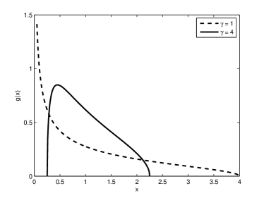
Figure 1: Limiting densities of the noise subspace eigenvalues for $\gamma=1$ and $\gamma=4$ cases. The spread of the eigenvalues around 1 is evident.

II-B2 The Tracy-Widom distribution

The largest eigenvalue of a complex correlation matrix in the null case has a bell-shaped distribution called $F_{2}$ with moments [11]

$$E(l_{1})\simeq\mu_{nL}-1.8\,\sigma_{nL}$$ (15)

$$\textrm{Std}(l_{1})\simeq 0.9\,\sigma_{nL}$$ (16)

in which

$$\mu_{nL}=\bigg{(}1+\sqrt{\frac{L}{n}}\,\bigg{)}^{2}$$ (17)

$$\sigma_{nL}=\sqrt{\frac{\mu_{nL}}{n}}\bigg{(}\frac{1}{\sqrt{n}}+\frac{1}{\sqrt{L}}\,\bigg{)}^{1/3}.$$ (18)

Let’s see a numerical example. Assume $n=100$ and $L=10$, then $E(l_{1})\simeq 1.55$ and $\textrm{Std}(l_{1})\simeq 0.09$ which implies that $l_{1}>1.3$ with high probability. We conclude that the signal eigenvalues should be well larger than $\sigma^{2}$.

III Probability of Missed Detection

III-A Method of Calculation

In this subsection, using the statistical tools developed in the previous section, we calculate $p_{m}$ for MDL method. $p_{fa}$ is negligible in moderate values of $n$ and $L$. For example, in $L=3$ and $n=30$, $p_{fa}\simeq 0.003$ and decays rapidly when $n$ and $L$ increase. $p_{m}$ can be used to estimate the minimum energy level of a source to be detectable by the system. It can also be used to determine the system capability for resolving very close sources. Then, we concentrate on the $p_{m1}\triangleq p_{m}(d=1)$ and $p_{m2}\triangleq p_{m}(d=2)$, although our method can be used for the general scenario. Let $H_{1}$ denote the situation in which only one source is present

$$p_{m1}=p\,\big{(}\Lambda(0,L,n)<\Lambda(1,L,n)\,|\,H_{1}\big{)}.$$ (19)

Using (5) and rearranging the terms in (19) we get

$$p_{m1}=p\,\big{(}L\log\bigg{(}\frac{a_{0}}{\,g_{0}}\bigg{)}-(L-1)\log\bigg{(}\frac{a_{1}}{g_{1}}\bigg{)}\qquad$$

$$<\frac{1}{2n}(2L-1)\log(n)\big{)}$$ (20)

By the definition of $a_{d}$ in (6), we can write

$$a_{0}=\frac{1}{L}\,l_{1}+\frac{L-1}{L}\,a_{1}$$ (21)

Similarly, for the geometric mean using (7) we have

$$g_{0}^{L}=l_{1}\,g_{1}^{L-1}$$ (22)

Substituting (21) and (22) in (III-A), we get [3]

$$p_{m1}=p\,\big{(}\log Q_{m1}\big{(}\textstyle{\frac{l_{1}}{a_{1}}}\big{)}<T_{1}\big{)}$$ (23)

where

$$Q_{m1}(x)\triangleq\frac{1}{x}\Big{(}\,1+\frac{x-1}{L}\,\Big{)}^{L}$$ (24)

and

$$T_{1}=\frac{1}{2n}(2L-1)\log(n)$$ (25)

In [3], The function $\log(Q_{m1}(x))$ is approximated by its second order Taylor series near $x=1$. This is one source of avoidable error in the method. The smallest eigenvalue of the signal subspace is greater than the largest eigenvalue of the noise subspace, which is, from subsection II-B, larger than $\sigma^{2}$. Also recall that $a_{1}\simeq\sigma^{2}$, we conclude that $x>1$. It is evident that the function $\log(Q_{m1}(x))$ is uniformly increasing in the region $x>1$, therefore we can translate the inequality in (23) to a simpler one

$$p_{m1}=p\,(x<T_{1\,x})$$ (26)

where

$$\log(Q_{m1}(T_{1\,x}))=T_{1}$$ (27)

Using (26), two steps are required for calculation of $p_{m}$, computing $T_{1\,x}$ from (27) and determining the statistics of $x\triangleq{l_{1}}/{a_{1}}$ in (26).

Unfortunately, (27) cannot be solved analytically for $T_{1\,x}$, then we find an approximate solution in the first step. Rearrange (27) to get

$$\bigg{(}1+\frac{T_{1x}-1}{L}\bigg{)}^{L}=T_{1x}\,e^{T_{1}}$$ (28)

Expanding the left-hand-side of (28) to the second order, assuming $L$ is sufficiently large and solving the resulting quadratic equation, gives a first approximation for $T_{1x}$

$$T_{1x}^{(1)}=1+\sqrt{e^{2T_{1}}-1}$$ (29)

Now since the function in L.H.S. of (27) is smooth, we can use a first order Taylor series around the solution in (29) to get closer to the exact solution

$$T_{1x}^{(i+1)}=T_{1x}^{(i)}+\big{(}\,T_{1}-T_{1}^{(i)}\big{)}\frac{T_{1x}^{(i)}+1}{T_{1x}^{(i)}-1}$$ (30)

where $T_{1}^{(i)}$ depends on $T_{1x}^{(i)}$ through (27). Application of (30) for a few times gives a very accurate solution. Note that computation of $T_{1x}$ is done after setting $n$ and $L$, but is not dependent on the SNR.

The next step in calculating $p_{m1}$ is determining the statistics of $x$. From (10) and (11), we can see that $l_{1}$ is distributed as

$$l_{1}\sim\;\mathcal{N}\bigg{(}\lambda_{1}+\frac{(L-1)\lambda_{1}\sigma^{2}}{n(\lambda_{1}-\sigma^{2})}\;\,,\;\frac{\lambda_{1}^{2}}{n}\bigg{)}$$ (31)

In [3, 5, 4, 8], the bias term of $l_{1}$ is not considered, while a numerical example can clarify the point. Assume that $n=100$, $L=10$, and $\sigma^{2}=1$. In the SNR in which $p_{m1}$ starts to become large, $\lambda_{1}=1.5$, $E(l_{1})=2.2$, and $\textrm{Std}(l_{1})=0.15$. Therefore, overlooking the bias term ($0.7$) introduces large error to the analysis. Since in the critical SNRs, the signal eigenvalue get closer to the noise eigenvalues, the denominator in (10) reduces and the bias term gets large.

In the null case, $E(a_{0})=\frac{1}{L}E(\textrm{Tr}(\hat{\boldsymbol{R}}))=\sigma^{2}=1$, which recommends that $E(a_{1}|H_{1})=\sigma^{2}$. But a signal eigenvalue can cause a negative bias on $a_{1}$, numerically about 2%. Then, although we neglect the variance of $a_{1}$ which is very small compared to the variance of $l_{1}$, we should take into account the bias to achieve an exact performance evaluation. In fact, the variances of the eigenvalues (regardless of being a noise eigenvalue or a signal one) increases with the mean of the eigenvalue. This can be seen in the simulations and can be justified for the noise eigenvalues with noticing the decay of the Marcenko-Pastur distribution in Fig. 1 which results in increasing variance of its order statistics. The variance of any order statistic of a distribution is inversely proportional to the squared value of the distribution in the vicinity of the mean value of that order statistics. A classical example of this fact is the variance of the median. For the signal eigenvalues, this is already shown in (11) and (13). This fact, along with the averaging in the calculation of $a_{1}$ shows that its variance is negligible in the analysis. To calculate the bias, note that $E(l_{1})+(L-1)E(a_{1})=E(\textrm{Tr}(\hat{\boldsymbol{R}}))=\textrm{Tr}(\boldsymbol{R})=\lambda_{1}+(L-1)\sigma^{2}$. This besides (10) gives [16]:

$$H_{1}\quad:\quad a_{1}\simeq\;\sigma^{2}-\frac{\sigma^{2}\lambda_{1}}{n(\lambda_{1}-\sigma^{2})}$$ (32)

Using (31) and (32), the distribution of $x$ is determined as a Gaussian random variable with known mean $\mu_{x}$ and variance $\sigma_{x}^{2}$. Then, $p_{m1}$ can be calculated as

$$p_{m1}=1-Q\bigg{(}\frac{T_{1x}-\mu_{x}}{\sigma_{x}}\bigg{)}$$ (33)

in which

$$Q(t)=\int_{t}^{\infty}\frac{1}{\sqrt{2\pi}}e^{-\frac{u^{2}}{2}}du.$$ (34)

The same procedure can be used to calculate $p_{m2}$. The following approximation is widely used and justified in the literature [3, eq. (24)], [5, eq. (II.3a)]:

$$p_{m2}\simeq p\,\big{(}\Lambda(1,L,n)<\Lambda(2,L,n)\,|\,H_{2}\big{)}$$ (35)

It basically states that the probability of missing one of the sources is very larger than missing both of them. We drop the details and just give some of the points important in the calculation of $p_{m2}$:

$$p_{m2}=p\,\big{(}\log Q_{m2}\big{(}\textstyle{\frac{l_{2}}{a_{2}}}\big{)}<T_{2}\big{)}$$ (36)

in which the threshold $T_{2}$ and the function $Q_{m2}$ are defined as

$$T_{2}=\frac{1}{2n}(2L-3)\log(n)$$ (37)

$$Q_{m2}(x)=\frac{1}{x}\,\Big{(}\,1+\frac{x-1}{L-1}\,\Big{)}^{L-1}$$ (38)

$$x\triangleq\frac{l_{2}}{a_{2}}$$ (39)

The recursive equation to estimate the threshold $T_{2x}$ will be

$$T_{2x}^{(i+1)}=T_{2x}^{(i)}+\big{(}T_{2}-T_{2}^{(i)}\big{)}\frac{\;T_{2x}^{(i)}(L-2+T_{2x}^{(i)})}{(L-2)(T_{2x}^{(i)}-1)}$$ (40)

The distribution of $l_{2}$ will be

$$l_{2}\sim\;\mathcal{N}\bigg{(}\lambda_{2}+\frac{(L-2)\lambda_{2}\sigma^{2}}{n(\lambda_{2}-\sigma^{2})}-\frac{\lambda_{1}\lambda_{2}}{n(\lambda_{1}-\lambda_{2})}\;\,,\;\frac{\lambda_{2}^{2}}{n}\bigg{)}$$ (41)

$a_{2}$ will have a negligible variance and can be estimated by its mean value:

$$H_{2}\quad:\quad E(a_{2})=\;\sigma^{2}-\frac{\sigma^{2}\lambda_{1}}{n(\lambda_{1}-\sigma^{2})}-\frac{\sigma^{2}\lambda_{2}}{n(\lambda_{2}-\sigma^{2})}$$ (42)

Now, using (41) and (42), the distribution of $x$ in (39) can be found and $p_{m2}$ is achieved as in (33). The same procedure can be used for determining $p_{m}$ in any number of sources.

III-B Deterministic Signal Model

Although the first- and second-order statistical properties of the signal subspace eigenvalues are different under stochastic and deterministic signal models, the performance of the MDL is the same under two models. As explained in section III-A, $p_{m}$ depends on the statistics of the weakest signal eigenvalue $l_{d}$. We show that these statistics grow similar under two models when $l_{d}$ approaches the noise eigenvalues. Note that, for a fair comparison of the two signal models, the signal second-order characteristics should be the same (see e.g. [9, sec. V]). Therefore, we have $\lim_{n\to\infty}\boldsymbol{S}_{\textrm{det}}\boldsymbol{S}_{\textrm{det}}^{\textrm{\,H}}/n=E(\boldsymbol{s}_{\textrm{sto}}\boldsymbol{s}_{\textrm{sto}}^{\textrm{H}})$, which results in $\boldsymbol{R}_{\textrm{det}}=\boldsymbol{R}_{\textrm{sto}}$ and hence $\lambda_{i\,\textrm{det}}=\lambda_{i\,\textrm{sto}},\;i=1,\ldots,L$. In the situations where $p_{m}$ starts to grow large, $l_{d}$ is barely larger than the noise eigenvalues, $\lambda_{d}\simeq\sigma^{2}$, then from (12) we have

$$E(l_{d\,\textrm{det}})\simeq\lambda_{d}+\sum_{i\neq d}\frac{\sigma^{2}\lambda_{i}}{n(\sigma^{2}-\lambda_{i})}$$ (43)

which is the same as (10) in stochastic signal model. For the variances, we assume that $\lambda_{d}$ has approached the upper limit of the noise eigenvalues

$$\lambda_{d}\simeq\sigma^{2}\bigg{(}1+\sqrt{\frac{L}{n}}\,\bigg{)}^{2}$$ (44)

which is the upper limit of the Marcenko-pastur distribution in (14). Note that, as signal power reduces, its eigenvalue approaches the noise eigenvalues roughly about $\sigma^{2}$. But $\lambda_{d}$ cannot be smaller than the largest noise eigenvalue due to the sorting of the eigenvalues. Then as the SNR reduces, $\lambda_{d}$ approaches the upper limit of the noise eigenvalues about (44). In fact, we are using a better approximation for $\lambda_{d}$ in calculating the variance in (44) rather than in calculating the expectation in (43). Assuming $L\ll n$, a first order expansion of (44) can be used in (11) to give

$$\textrm{Var}_{\textrm{sto}}\,(l_{d})=\frac{1}{n}\,\lambda_{d}^{2}\simeq\frac{1}{n}\,\sigma^{4}\bigg{(}1+4\sqrt{\frac{L}{n}}\;\bigg{)}$$ (45)

and in (13) to give

$$\textrm{Var}_{\textrm{det}}\,(l_{d})=\frac{1}{n}\,\big{(}2\lambda_{d}\sigma^{2}-\sigma^{4}\big{)}\qquad\qquad\qquad\qquad$$

$$\simeq\frac{1}{n}\,\sigma^{4}\bigg{[}2\bigg{(}1+2\sqrt{\frac{L}{n}}\;\bigg{)}-1\bigg{]}$$ (46)

which reduces to the result in (45) and we can conclude that the variance of $l_{d}$ is the same under two models in low SNRs. Hence, $p_{m}$ is approximately the same under two signal models. This is in harmony with the same result in the DOA estimation problem, where the performance of the estimators are the same under two signal model [9].

IV Simulation Results

In this section, simulation results are presented to support the theoretical derivations. We consider $p_{m}$ in different conditions of number of snapshots $n$, and number of sensors $L$ in a Uniform Linear Array with half-wavelength inter-element distance. Our estimate is compared with [3] and [8]. Results are presented for two closely spaced sources in $p_{m2}$, and one source in $p_{m1}$. When the sources get closer to each other, the weaker signal eigenvalue approaches the noise eigenvalues and possibly miss will occur. Therefore, for a fixed angular distance of the sources, a minimum SNR is required for the array to be able to detect both sources.

Two equally powered uncorrelated signal sources in $\pm 2^{o}$ are assumed. The SNR is defined as the ratio of each signal variance to noise variance (i.e. sensor SNR).

Figure 2: $p_{m2}$ of MDL method when number of sensors $L=10$, and number of snapshots $n=100$.

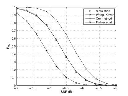
Figure 3: $p_{m2}$ of MDL method when number of sensors $L=10$, and number of snapshots $n=900$.

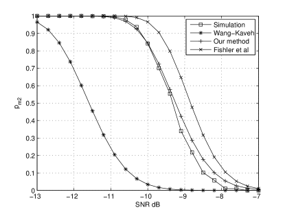
Figure 4: $p_{m2}$ of MDL method when number of sensors $L=32$, and number of snapshots $n=64$.

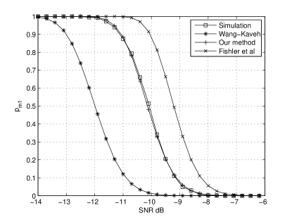
Figure 5: $p_{m1}$ of MDL method when number of sensors $L=32$, and number of snapshots $n=64$.

Figs 2, 3, and 4 show the corresponding results for $p_{m2}$ different situations in terms of $n$ and $L$. Fig. 5 presents the results for $p_{m1}$ in the worst case of parameters. The superiority of our method in estimating the simulation results is evident. In Fig. 2, simulation results are presented for both deterministic and stochastic signals, which confirms the approximate equality of $p_{m}$ under two models. This equality improves as the number of observations $n$ increases. Note that our method is used to estimate $p_{m}$ under stochastic signal model in Fig. 2. The analysis in [3] under-estimates $p_{m}$ with a horizontal distance of about 0.5-2 dB. In fact, this method improves when $n$ gets larger since in this situation, the neglected biases reduce. The estimate of [8] is better than [3], with over-estimation of $p_{m}$ equivalent with a horizontal distance about 0.5-1 dB. Note that in the extreme case of $L=32$ and $n=64$ of Fig. 4, our analysis starts to degrade since the asymptotic assumption is no longer valid. Though, in most cases, our estimate exhibits horizontal distance of about 0.03 dB.

We have seen that the analysis in [3, 4, 5] lacks the inclusion of biases of the eigenvalues and also suffers from some inaccurate approximations. But the analysis in [8] requires more scrutiny since as we have seen in the simulation results, this analysis gives completely different results from [3]. Authors in [8] use asymptotic conditions to show that $\Lambda(d-1)-\Lambda(d)$ converges in distribution to a Gaussian random variable with mean $\mu$ and variance $\sigma^{2}$. Simulations show that although the formula derived for $\sigma^{2}$ in [8] is a very good estimate of the empirical value, the same is not true for the mean $\mu$, which in fact shows considerable deviation. This disagreement is present in small $n$ as well as large $n$ conditions. The derived result for the mean of the Gaussian distribution in [8, eq. (19)] is

$$\mu=n\log\bigg{(}\frac{\sigma_{n}^{2}}{\lambda_{d}}\bigg{[}1+\frac{1}{L-d+1}\Big{(}\,\frac{\lambda_{d}}{\sigma_{n}^{2}}-1\Big{)}\bigg{]}^{L-d+1}\,\bigg{)}$$

$$+\;0.5\Big{(}2d-2L-1\Big{)}\log(n)$$ (47)

which we can see that is $n\log Q_{md}(x)$ plus some nonrandom term in the notation of our analysis. Now, it is evident that (IV) is derived assuming $E(l_{i})=\lambda_{i}$ for signal subspace and $E(a_{d})=\sigma_{n}^{2}$, thus every biases in the distribution of $l_{i}$ and $a_{d}$ is ignored. Additionally, Although we can assume the distribution of $x$ to be Gaussian, it is not easy to assume normality for the function $\Lambda(d-1)-\Lambda(d)$ since it is a highly nonlinear function of $x$. Simulations show that the normality assumption is approximately valid only for large values of $n$, say $n\simeq 1000$. Another issue is that nonlinearity of the function $\log(Q_{md}(x))$ move the mean of the distribution which is not taken into account.

Here, we will give further simulation results that compare our analysis with the one presented in [8]. We assume the same conditions as in [8, Fig. 1] which is $n=900$, $L=7$, and two Gaussian sources in $\boldsymbol{\theta}=[-5^{o}\;\,+10^{o}]$.

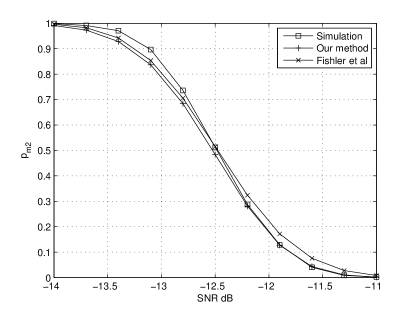
Figure 6: $p_{m2}$ of MDL method when number of sensors $L=7$, and number of snapshots $n=900$. The performance prediction method in [8] works well in this set of parameters.

The results are shown in Fig. 6, where the experimental performance of MDL method is accurately predicted by both our method and the method presented in [8]. Although from a theoretical point of view, the method of [8] is not comprehensive enough, in this special case of parameters it works well. If we change the sources DOAs and keep every other parameters unchanged we will see that the predictions of [8] degrades.

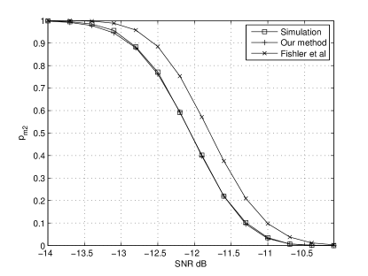
Figure 7: $p_{m2}$ of MDL method when number of sensors $L=7$, and number of snapshots $n=900$. The performance prediction method in [8] does not work well in this set of parameters.

Figure 7 shows the experimental results and theoretical predictions when sources are in $\boldsymbol{\theta}=[-5^{o}\;\,20^{o}]$. It is evident that the method of [8] does not work well anymore while our method is still accurate. Note that we have investigated its performance when sources are very close to each other in our previous simulation results where the method in [8] failed to predict the performance accurately. Therefore, the method in [8] cannot be a reliable method of analytical performance calculation.

V Conclusion

An accurate performance analysis for the probability of missed detection of the MDL source enumeration method was presented. Statistical characterization of the principal components of the covariance matrix helped to take good assumptions and approximation which resulted in improved estimations of $p_{m}$. It is proved that the performance is approximately identical under stochastic and deterministic signal models using a perturbation analysis which gives the statistical properties of eigenvalues in the deterministic signal model. Simulation results show the superiority of the proposed analysis compared with the previous results.

Appendix A Proof of Lemma 1

Let $\boldsymbol{X}\triangleq\boldsymbol{Y}-\boldsymbol{\mu}$ and rearrange the covariance in (1) as

$$n^{2}c=\textrm{Cov}(\boldsymbol{\alpha}^{\textrm{H}}\boldsymbol{XX}^{\textrm{H}}\boldsymbol{\beta}+\boldsymbol{\alpha}^{\textrm{H}}\boldsymbol{\mu X}^{\textrm{H}}\boldsymbol{\beta}+\boldsymbol{\alpha}^{\textrm{H}}\boldsymbol{X\mu}^{\textrm{H}}\boldsymbol{\beta}$$

$$,\boldsymbol{\gamma}^{\textrm{H}}\boldsymbol{XX}^{\textrm{H}}\boldsymbol{\zeta}+\boldsymbol{\gamma}^{\textrm{H}}\boldsymbol{\mu X}^{\textrm{H}}\boldsymbol{\zeta}+\boldsymbol{\gamma}^{\textrm{H}}\boldsymbol{X\mu}^{\textrm{H}}\boldsymbol{\zeta}).$$ (48)

Circularity of the distribution and zero odd moments of zero-mean Gaussian distribution reduces (A) to

$$n^{2}c=\textrm{Cov}(\boldsymbol{\alpha}^{\textrm{H}}\boldsymbol{XX}^{\textrm{H}}\boldsymbol{\beta}\,,\boldsymbol{\gamma}^{\textrm{H}}\boldsymbol{XX}^{\textrm{H}}\boldsymbol{\zeta})$$

$$+\>\textrm{Cov}(\boldsymbol{\alpha}^{\textrm{H}}\boldsymbol{\mu X}^{\textrm{H}}\boldsymbol{\beta}\,,\boldsymbol{\gamma}^{\textrm{H}}\boldsymbol{\mu X}^{\textrm{H}}\boldsymbol{\zeta})$$

$$+\>\textrm{Cov}(\boldsymbol{\alpha}^{\textrm{H}}\boldsymbol{X\mu}^{\textrm{H}}\boldsymbol{\beta}\,,\boldsymbol{\gamma}^{\textrm{H}}\boldsymbol{X\mu}^{\textrm{H}}\boldsymbol{\zeta}).$$ (49)

The first term in (A) is given by (8). The fact that $\boldsymbol{x}_{i}\perp\boldsymbol{x}_{j}:i\neq j$ reduces the second term as

$$\boldsymbol{\alpha}^{\textrm{H}}\!\boldsymbol{\mu}\,E(\boldsymbol{X}^{\textrm{H}}\boldsymbol{\beta\,\zeta}^{\textrm{H}}\boldsymbol{X})\,\boldsymbol{\mu}^{\textrm{H}}\boldsymbol{\gamma}=$$

$$\boldsymbol{\alpha}^{\textrm{H}}\!\boldsymbol{\mu}\,\textrm{diag}(E(\boldsymbol{x}_{i}^{\textrm{H}}\boldsymbol{\beta\,\zeta}^{\textrm{H}}\boldsymbol{x}_{i}))\,\boldsymbol{\mu}^{\textrm{H}}\boldsymbol{\gamma}=$$

$$(\boldsymbol{\alpha}^{\textrm{H}}\boldsymbol{\mu\mu}^{\textrm{H}}\,\boldsymbol{\gamma})(\boldsymbol{\zeta}^{\textrm{H}}\boldsymbol{\Sigma}\,\boldsymbol{\beta}).$$ (50)

The third term in (A) can be derived in the same way. Note that all the three terms in the right-hand-side of (1) are $\mathcal{O}({n^{-1}})$ since $\boldsymbol{\mu}$ is of dimension $L\times n$ and hence $\boldsymbol{\mu\mu}^{\textrm{H}}$ is $\mathcal{O}({n})$.

Appendix B Proof of Theorem 2

In the asymptotic region of $n\gg 1$, $\hat{\boldsymbol{R}}$ is a slightly perturbed version of $\boldsymbol{R}$, described as

$$\hat{\boldsymbol{R}}=\boldsymbol{R}+p\boldsymbol{\Delta}$$ (51)

where $p\ll 1$ is the perturbation factor. Small perturbations in $\boldsymbol{R}$ result in small changes in its eigenvectors if the associated eigenvalues are sufficiently separated [12]. It means that the following results are true for signal eigenvalues. Remember the definition of the eigendecompositions as $\boldsymbol{Rv}_{i}=\lambda_{i}\boldsymbol{v}_{i}$ and $\hat{\boldsymbol{R}}\boldsymbol{w}_{i}=l_{i}\boldsymbol{w}_{i}$. The first order perturbation in eigenvectors is

$$\boldsymbol{w}_{i}\simeq\boldsymbol{v}_{i}+\sum_{j\neq i}t_{ij}p\,\boldsymbol{v}_{j}$$ (52)

where $t_{ij}$s are the perturbation coefficients. Straightforward calculations will give [13, eq. (A.9)][14]:

$$l_{i}=\lambda_{i}+p\,\boldsymbol{v}_{i}^{\textrm{H}}\!\boldsymbol{\Delta\,v}_{i}+\sum_{j\neq i}t_{ij}p^{2}\boldsymbol{v}_{i}^{\textrm{H}}\boldsymbol{\Delta\,v}_{j}$$ (53)

$$t_{ij}=\frac{\boldsymbol{v}_{j}^{\textrm{H}}\boldsymbol{\Delta\,v}_{i}}{\lambda_{i}-\lambda_{j}}.\qquad\qquad\qquad$$ (54)

Under the conditions of Theorem 2, we will have

$$\textrm{Cov}\big{(}\,t_{ik},t_{jr}\big{)}=\delta_{ij}\,\delta_{kr}\frac{(\lambda_{i}+\lambda_{k})\,\sigma^{2}-\sigma^{4}}{np^{2}(\lambda_{i}-\lambda_{k})^{2}}\qquad$$ (55)

which is shown using (54) and replacing $\boldsymbol{\mu\mu}^{\textrm{H}}=n(\boldsymbol{R}-\sigma^{2}\boldsymbol{I})$ in (1). Now, (12) is proved using (53) and (1). (13) can be shown using (53) to the first order and (1). Note that the limiting distribution of the eigenvalues is Gaussian [9].

References

- [1] M. Wax and T. Kailath, ”Detection of signals by information theoretic criteria,” IEEE Trans. Acoustic Speech Signal Process., vol. ASSP-33, pp. 387-392, Apr. 1985.
- [2] A.P. Liavas, P.A. Regalia, and J.P. Delmas, “Blind channel approximation: Effective channel order determination,” IEEE Trans. Signal Process., vol. 47, pp. 3336-3344, Dec. 1999.
- [3] H. Wang and M. Kaveh, ”On the performance of signal-subspace processing - part I: narrow-band systems,” IEEE Trans. Acoust. Speech, Signal Process., vol. ASSP-34, pp. 1201-1209, Oct. 1986.
- [4] M. Kaveh, H. Wang, and H. Hung, ”On the theoretical performance of a class of estimators of the number of narrow-band sources,” IEEE Trans. Acoust. Speech, Signal Process., vol. ASSP-35, pp. 1350-1352, Sep. 1987.
- [5] Q. Zhang, K. M. Wong, P. C. Yip, and J. P. Reilly, ”Statistical analysis of the performance of information theoretic criteria in the detection of the number of signals in array processing,” IEEE Trans. Acoustic Speech Signal Process., vol. 37, pp. 1557-1567, Oct. 1989.
- [6] W. Xu and M. Kaveh, ”Analysis of the performance and sensitivity of eigendecomposition-based detectors,” IEEE Trans. Signal Process., vol. 43, pp. 1413-1426, June 1995.
- [7] A.P. Liavas, P.A. Regalia, ”On the behavior of information theoretic criteria for model order selection” IEEE Trans. Signal Process., vol. 49, pp. 1689-1695, August 2001.
- [8] E. Fishler, M. Grossmann, and H. Messer, ”Detection of signals by information theoretic criteria: general asymptotic performance analysis,” IEEE Trans. Signal Process., vol. 50, pp. 1027-1036, May 2002.
- [9] B. Ottersten, M. Viberg, and T. Kailath, ”Analysis of subspace fitting and ML techniques for parameter estimation from sensor array data”, IEEE Trans. Signal Process., vol. 40, pp. 590-599, March 1992.
- [10] D. R. Brillinger, Time Series: Data Analysis and Theory. New York: Holt, Rinehart, and Winston, 1975.
- [11] I. M. Johnstone, ”On the distribution of the largest eigenvalue in principal component analysis,” Annals of Statistics, vol. 29, No. 2, pp. 295-327, 2001.
- [12] G. H. Golub and C. F. Van Loan, Matrix Computations, The Johns Hopkins University Press, 1989.
- [13] M. Kaveh and A. J. Barabell, “The statistical performance of the MUSIC and the minimum-norm algorithms in resolving plane waves in noise,” IEEE Trans. Acoust. Speech, Signal Process., vol. ASSP-34, pp. 331-341, April 1986.
- [14] J. H. Wilkinson, The Algebraic Eigenvalue Problem. New York: Oxford University Press, 1965.
- [15] D. Lawley, ”Tests of significance for the latent roots of covariance and correlation matrices,” Biometrika. vol. 43, pp. 128-136, 1956.
- [16] K. M. Wong, Q. Zhang, J. P. Reilly, and P. C. Yip, ”On information theoretic criteria for determining the number of signals in high resolution array processing,” IEEE Trans. Acoust. Speech, Signal Process., vol. 38, pp. 1959-1971, Nov. 1990.