Finite-size anisotropy in statistically uniform porous media

Abstract

Anisotropy of the permeability tensor in statistically uniform porous media of sizes used in typical computer simulations is studied. Although such systems are assumed to be isotropic by default, we show that de facto their anisotropic permeability can give rise to significant changes of transport parameters such as permeability and tortuosity. The main parameter controlling the anisotropy is $a/L$, being the ratio of the obstacle to system size. Distribution of the angle $\alpha$ between the external force and the volumetric fluid stream is found to be approximately normal, and the standard deviation of $\alpha$ is found to decay with the system size as $(a/L)^{d/2}$, where $d$ is the space dimensionality. These properties can be used to estimate both anisotropy-related statistical errors in large-scale simulations and the size of the representative elementary volume.

I Introduction

A standard method of modeling a uniform, isotropic porous medium (e.g. a column of sand) is to place randomly many identical objects that are impermeable to fluid (e.g. solid spheres) in an initially empty volume Martys and Garboczi (1992); Koponen et al. (1997); Nabovati and Sousa (2007); Verberg and Ladd (1999); Kostek et al. (1992); Matyka et al. (2008); Başagaoglu et al. (2006); Zhang and Knackstedt (1995). Since the objects are placed uniformly in the whole system, one might expect that randomness in their exact locations is irrelevant in the sense that the bulk volumetric fluid stream will be parallel to the external force (e.g. gravitation). This would be the case if the system was large enough. However, in computer simulations and in artificial laboratory systems (used in particle image velocimetry measurements Zerai et al. (2005)), usually relatively small systems are utilized that contain at most a few thousands of ”grains”—far less than billions of sand grains in a typical experimental setup. Since randomly distributed grains tend to form channels of random orientations, small porous systems are very sensitive to local fluctuations of the grain distribution. Under such conditions the direction of the volumetric fluid stream can differ significantly from that of the external force. Consequently, a system that was supposed to be isotropic, may de facto be rather highly anisotropic. The aim of this paper is a detailed analysis of this phenomenon in a two-dimensional (2D) flow.

A porous medium is anisotropic to flow if the permeability tensor is anisotropic. Usually anisotropy of the permeability tensor is either assumed explicitly Bear (1972) or it appears naturally as an expected consequence of a microscopic model Scholes et al. (2007); Boudreau and Meysman (2006); Alam et al. (2006); Ohkubo (2008). In the former case one works entirely on a macroscopic level, whereas the latter approach tries to connect the observed macroscopic anisotropy of real porous materials with their microscopic geometry and structure. Permeability anisotropy caused by a finite size of a model system has not been regarded as an important factor so far, although some research techniques, e.g. numerical simulations, concentrate on artificially small porous systems. The reason for this lies in the fact that numerical flow simulations in complex porous geometries are extremely tedious and require extensive computer power and resources. A common strategy has been to perform calculations for just a few systems that are as large as possible Cancelliere et al. (1990); Başagaoglu et al. (2006). In contrast to this, here we solve the flow equations for hundreds or even thousands of different porous systems of small to medium sizes and then extrapolate the results to the limit of an infinitely large system. This method was already used in Matyka et al. (2008) to detect a small, systematic deviation of the flow tortuosity from several theoretical formulas, with an ad hoc interpretation of this phenomenon as a consequence of the finite-size anisotropy. Therefore, in this paper we present a systematic study of finite-size anisotropy in a two-dimensional model of statistically uniform porous media.

The structure of the paper is as follows. Section II specifies the model and the numerical techniques used. Main results are provided in Sec. III. Next, in Section IV we develop a simple theory to account for the asymptotic behavior of the angle between the external force and the volumetric fluid flux. Finally, the results are discussed in Sec. V.

II Model

In this study we use a model of freely overlapping squares Koponen et al. (1996, 1997); Matyka et al. (2008). In essence, this is a two-dimensional lattice model with a porous matrix modelled as a union of freely overlapping identical solid squares of size $a\times a$ lattice units (l.u.) placed uniformly at random locations in a square lattice $L\times L$ l.u. ($1\leq a\ll L$). The squares are fixed in space but free to overlap, and their sides coincide with the underlying lattice. The remaining void space is filled with a fluid. A constant, external force is imposed on the fluid to model the gravity and we allow an angle ($\beta$) between the force and the system side to be arbitrary (note that in Koponen et al. (1996, 1997); Matyka et al. (2008) only the case $\beta=0$ was considered). Periodic boundary conditions are imposed in both directions to minimize finite-size effects. The porosity ($\phi$) is calculated as the ratio of unoccupied lattice nodes to the entire system volume ($L^{2}$). The flow equations are solved in the creeping flow regime using the Lattice Boltzmann Model (LBM) Succi (2001) with a single relaxation time collision operator Bhatnagar et al. (1954) (see Matyka et al. (2008) for implementation details).

The model has three adjustable parameters: $\phi$, $a$, and $L$. The first one corresponds directly to the macroscopic porosity. The value of $a$ affects the percolation threshold $\phi_{c}$, which is a decreasing function of $a$ from $\phi_{c}\approx 0.4073$ (the standard site percolation threshold, $a=1$) Sahimi (1993) to $\phi_{c}\approx 0.3333$ (the continuous percolation threshold of aligned squares, $a\to\infty$) Baker et al. (2002). As the model is solved using the LBM method without a numerical grid refinement Matyka et al. (2008), the minimum value of $a$ is 4 (this is the minimum length scale for the LBM method to resolve the macroscopic Navier-Stokes equations Succi (2001)). The value of $L$ controls the finite-size effects through the dimensionless ratio $a/L$, which should be as small as possible to mimic an infinite system.

Anisotropy of fluid flow in the above-defined model will be investigated through Darcy’s law Bear (1972)

$$\bm{q}=\bm{K}\hat{\bm{g}},$$ (1)

where ${\bm{q}}$ is the volumetric fluid flux, $\bm{K}$ is a symmetric tensor of the hydraulic conductivity, and $\hat{\bm{g}}$ is the unit vector in the direction of the gravitational field.

III Numerical results

III.1 Tests on $\bm{K}$

The basic concept of transition from microscopic laws of hydrodynamics to macroscopic laws of transport in porous media is the representative elementary volume (REV), i.e. the smallest volume such that a measurement over it will yield a value representative of the whole Bear (1972). Darcy’s law (1) is, in principle, applicable only to systems that are larger than an REV, whereas significant anisotropy is expected in systems smaller than an REV. Hence, the primary question is whether or not Eq. (1) can be used to study anisotropy in small-size systems. To answer this we performed several simulations on $\bm{K}$, with its elements computed from $\bm{q(\hat{g})}$ for $\bm{\hat{g}}=\bm{\hat{x}}$ and $\bm{\hat{g}}=\bm{\hat{y}}$.

First, the symmetry of $\bm{K}$ was examined by quantifying the value of a dimensionless parameter given by

$$\epsilon=\frac{|K_{xy}-K_{yx}|}{K_{xx}+K_{yy}}.$$ (2)

Furthermore, by choosing $L=100$ l.u., $a=4$ l.u., and $\phi=0.7,0.9$, eighty different (i.e., fourty systems for each $\phi$) statistically uniform porous systems were constructed, for which $\epsilon<$ 0.5% was found. This ensures that $\bm{K}$ is symmetric within $0.5\%$ numerical errors in its elements. In a subsequent analysis we enforced $\bm{K}$-symmetry via replacing its off-diagonal elements ($K_{xy}$ and $K_{yx}$) by their arithmetic mean, which ensures that $\bm{K}$ is diagonizable.

Second, the tensorial properties of $\bm{K}$ were examined by checking whether Eq. (1) can be used for an arbitrary $\bm{\hat{g}}$. In particular, this equation predicts that if the mean flow direction ($\bm{q}$) is aligned with the $x$-axis, the angle $\beta$ between the external force ($\bm{{g}}$) and the $x$-axis should satisfy

$$\tan\beta=-\frac{K_{xy}}{K_{yy}}.$$ (3)

This relation was examined for several systems, of which one is shown in Fig. 1, wherein, two streamline patterns for the same system ($L=100$ l.u., $a=4$ l.u., $\phi=0.7$) with different $\bm{g}$-orientations are visualized. In the left panel, the external force is parallel to the (horizontal) $x$-axis ($\bm{\hat{g}}=\bm{\hat{x}}$), resulting in an angle of $\alpha\approx 21^{\circ}$ between the vector of the specific discharge ($\bm{q}$) and the $x$ axis.

In the right panel, a force of the same magnitude makes an angle $\beta\approx-22^{\circ}$ computed from (3); as expected, the angle between $\bm{\hat{q}}$ and the $x$ axis practically vanishes ($\alpha\approx-0.7^{\circ}$).

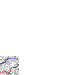
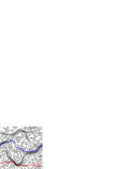
Figure 1: Streamlines through the same porous system ($L=100$ l.u., $a=4$ l.u., $\phi=0.7$) for two different alignments of the external force $\bm{g}$. The grey squares represent the solid part of the medium, and the remaining space is open to fluid flow. Left panel: $\bm{\hat{g}}$ is parallel to the $x$ axis ($\beta=0$) and the specific discharge $\bm{q}$ makes an angle $\alpha\approx 21^{\circ}$ with $\bm{\hat{x}}$. Right panel: $\beta\approx-22^{\circ}$ (calculated from Eq. (3)) and the angle between the specific discharge $\bm{q}$ and the $x$ axis is $\alpha\approx 0.7^{\circ}$. For the ease of display, two selected streamlines and their counterparts in both panels are given in color.

III.2 Tests on $\alpha$

A natural measure of anisotropy for a particular porous system is the angle between the vectors $\bm{\hat{g}}$ and $\bm{q}$. As this angle depends on the orientation of $\bm{\hat{g}}$, following standard procedures in computer simulations, we fix $\bm{\hat{g}}=\bm{\hat{x}}$. We verified that in this case the numerical value of $\alpha$ (angle between $\bm{q}$ and $\bm{\hat{g}}$) satisfies $\langle\alpha\rangle\approx 0$, which follows from symmetry arguments, and then calculated

$$\sigma_{\alpha}=\sqrt{\langle\alpha^{2}\rangle}.$$ (4)

In the above equation, $\langle\cdots\rangle$ denotes an average over different random porous systems. The results for $a=4$ l.u., $\phi=0.7,0.9$, and several system lengths $L$ are shown in Fig. 2. For $L\geq 100$ l.u. the data were fitted to

$$\sigma_{\alpha}\propto L^{-\delta},$$ (5)

which yielded $\delta\approx 0.96(6)$ for $\phi=0.7$ and $\delta\approx 1.00(3)$ for $\phi=0.9$. This suggests $\delta=1$, i.e.

$$\sigma_{\alpha}\propto L^{-1},\quad L\gg 1.$$ (6)

This relation does not hold for small $L$ ($L\lesssim 50$ in Fig. 2), for some realizations of such systems are likely to exhibit extreme anisotropy with $\alpha$ so large that $\sin\alpha$ cannot be approximated by $\alpha$ (for $L=50$ the angle between $\bm{q}$ and $\bm{\hat{g}}$ can be as large as $45^{\circ}$).

Figure 2: $\sigma_{\alpha}=\sqrt{\langle\alpha^{2}\rangle}$ as a function of $L$ for $a=4$ l.u. and two porosities $\phi=0.7,0.9$, with error bars at 95% confidence level. The lines represent fits to the power law $\sigma_{\alpha}\propto L^{-1}$ for $L\geq 100$ l.u.

Next we investigated statistical distribution of $\alpha$-values in different random systems with fixed $L$, $a$, and $\phi$. In all cases this distribution closely resembled the normal distribution $N(0,\sigma_{\alpha}^{2})$. Qualitative verification of this conjecture is presented in Fig. 3, which depicts the empirical cumulative distribution function (CDF) for two different system sizes $L$ (small symbols) together with the corresponding theoretical CDFs of the normal distribution,

$$F(\alpha)=\frac{1+\mathrm{erf}\,(\alpha/\sqrt{2}\sigma_{\alpha})}{2}.$$ (7)

The numerical data are in good agreement with (7). A quantitative comparison of the $\alpha$-distribution with $N(0,\sigma_{\alpha}^{2})$ was performed using the Kolmogorov-Smirnov test (at confidence level 95%). Out of all data points shown in Fig. 2 only the one corresponding to $L=50$ and $\phi=0.7$ did not pass the test, which in part is due to extremely large number of different samples (2000) used.

Figure 3: Cumulative distribution function (CDF) of $\alpha$ for $\phi=0.7$, $a=4$ l.u. and two system sizes $L=100$ and $L=400$ l.u. (dots). The empirical CDF was determined using 500 (for $L=100$) and 80 ($L=400$) numerical samples. Solid lines represent theoretical CDF of the normal distribution, Eq. (7), with $\sigma_{\alpha}=\sqrt{\langle\alpha^{2}\rangle}$.

As mentioned before, the value of $a$ determines the percolation threshold $\phi_{c}$ for small porosities, and can be considered as a relevant parameter independent of $\phi$ and $L$. For porosities much larger than $\phi_{c}$, however, the connectedness and overlapping of individual randomly generated solid squares becomes irrelevant. In this case, using scaling arguments, one can expect that $\phi$ and $a/L$ are the only relevant parameters. Mathematically, this can be formulated as a similarity ansatz:

$$\sigma_{\alpha}(a,L,\phi)\approx\Psi(a/L,\phi),\quad\phi\gg\phi_{c},L\gg a.$$ (8)

where $\Psi$ is a similarity function. A direct numerical verification of this conjecture is difficult, as it requires averaging over many independent samples, which is rather a time-consuming job for large $a$. Instead of this, we concentrated on a single parameter set with $\phi=0.7$ and $a/L=0.04$ that led to results demonstrated in Fig. 4

Figure 4: $\sigma_{\alpha}$ as a function of $a$ for $\phi=0.7$ and $a/L=0.04$ ($\times$ symbols). The data come from $N=500$ independent porous systems for $a\leq 4$ l.u. and $N=200$ for $a>4$ l.u. The error bars were calculated at the 95% confidence level. The solid line represents the best fit to Eq. (9).

shown as cross symbols. These data were fitted to an ad-hoc formula

$$\sigma_{\alpha}(a)=c_{1}+c_{2}\exp(-a/c_{3})$$ (9)

with three adjustable parameters $c_{1}$, $c_{2}$, and $c_{3}$. The best-fit value of $c_{3}\approx 0.6$ indicates that the approximation (8) can be safely used for $a\gtrsim 4$.

Finally, we investigated the dependence of $\sigma_{\alpha}$ on porosity. One expects that $\sigma_{\alpha}$ should decrease from $\approx 45^{\circ}$ at the percolation threshold $\phi_{c}$ (a single, randomly oriented conducting channel) to $0^{\circ}$ at $\phi=1$ (completely permeable system). As shown in Fig. 5, our numerical results generally agreed with this picture. However, $\sigma_{\alpha}$ did not converge to its limiting value $0$ as $\phi\to 1$. Instaed, it saturated at a positive value, which is independent of $\phi$. Due to this rather unexpected result, we ensured that neither discretization errors nor large relaxation times affect the numerical data obtained for large porosities. We also verified that the system size used, $L=100$, is sufficiently large for relation (6) to hold. This is clearly seen in the inset of Fig. 5, which depicts the product $\sigma_{\alpha}L$ for $L=100$ and $L=200$. The data for different $L$ collapsed in a broad range of $\phi\gtrsim 0.55$. Porosities less than $\approx 0.55$ are in a vicinity of the percolation critical point, at which $\sigma_{\alpha}$ is expected to converge to $45^{\circ}$ as $L\to\infty$, and hence the product $\sigma_{\alpha}L$ should diverge at $\phi_{c}$. As the system size $L\to\infty$, it is possible that the the porosity range, for which scaling relation (6) does not hold, diminishes according to a power law. This behavior is a typical finite-size effect near a critical point Hunt (2005).

Figure 5: $\sigma_{\alpha}$ (in degrees) as a function of porosity $\phi$ for $L=100$ l.u. Inset: the product $\sigma_{\alpha}L$ (deg. $\times$ l.u.) for $L=100$ l.u. (cross symbols) and $L=200$ l.u. (circle symbols). All data obtained for $a=4$ l.u.; error bars at 95% confidence level obtained from 200 independent porous systems. The arrows show the percolation threshold $\phi_{c}\approx 0.417$. Filled circles show theoretical values of $\sigma_{\alpha}$ for $\phi=\phi_{c}$, $L\to\infty$ ($45^{\circ}$) and $\phi=1$ ($0^{\circ}$).

To explore the reason why $\sigma_{\alpha}$ does not tend smoothly to 0 as $\phi$ approaches 1, we inspected the streamlines in high-porosity systems exhibiting large anisotropy. An extreme example of such a system, generated with $\phi=0.95$, is shown in Fig. 6a. At this high porosity, overlapping of individual obstacles is negligible, and the solid part of the system is made up of separate islands (that could correspond, for example, to a cross-section of a porous medium made of parallel fibers Koponen et al. (1998); Araújo et al. (2006)). Because the obstacles were placed uniformly and randomly in the whole system, their local concentration varies, and they form several larger groups of obstacles with relatively small distances between group members. Since fluid flux through a 2D channel is proportional to its width squared, most of the fluid flow takes place in relatively wide ‘channels’ between the groups. In other words, owing to no-slip boundary conditions on the obstacle surfaces, the fluid passes most easily in the inter-connected regions of low local obstacle concentration (high local porosity), whereas the regions of high local obstacle concentration (low local porosity)—even if occupied by separate obstacles—act effectively as large, almost impenetrable barriers. This solid-fluid ‘repulsion’ effect is not present in electric current flows (for the current intensity is proportional to the first power of a conductive channel width). For this reason, a high-porosity system which is highly anisotropic to fluid flow ($\alpha\approx 15^{\circ}$ in Fig. 6a) exhibits a marginal anisotropy to electric current flow ($|\alpha|<1^{\circ}$) as depicted in Fig. 6b.

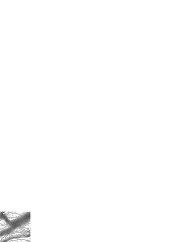
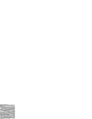
Figure 6: Streamlines in a high-porosity system ($\phi=0.95$) with $L=100$ l.u. and $a=4$ l.u. for two different flow types: (a) hydrodynamic ($\alpha\approx 15^{\circ}$); (b) electric ($\alpha\approx 0.6^{\circ}$). The electric flow was calculated from a solution of the Laplace equation with periodic boundary conditions and a constant electric field parallel to the $x$-axis. Note that the distribution of obstacles and the orientation of an external body force is identical in both panels.

III.3 Tests on principal values

Mathematically, a porous system is anisotropic to flow if and only if at least two of the principal values of $\bm{K}$ are diffrent. In the present case $\bm{K}$ has two eigenvalues (principal permeabilities) $K^{+}$ and $K^{-}$ which can be ordered such that $K^{+}\geq K^{-}$. Their ratio,

$$0\leq r=\frac{K^{-}}{K^{+}}\leq 1,$$ (10)

is equivalent to the ratio of the minimum to maximum permeabilities of a given porous system, and hence is a proper measure of its anisotropy Scholes et al. (2007). The more $r$ deviates from $1$, the more anisotropic the system is.

We first verified that, as expected, the angle between the main principal axis and the $x$-axis was distributed uniformly in the range $(-\pi/2,\pi/2]$ (data not shown). Then the CDF of $r$ was determined for a particular case with $\phi=0.7$, $a=4$ l.u., and $L=100$ l.u. As can be seen in Figure 7, the distribution of $r$ can be quite well fitted to the normal distribution $N(0.75,0.12^{2})$. However, this is only an approximation, as in the present case $\mathrm{CDF}(r)\equiv 1$ for $r\geq 1$.

Figure 7: Cumulative distribution function of $r=K^{-}/K^{+}$ for $\phi=0.7$, $a=4$ l.u., $L=100$ l.u., calculated using $N=340$ different porous systems. Dashed line represents the best fit to the CDF of the normal distribution with $\langle r\rangle\approx 0.75$ and $\sigma_{r}\approx 0.12$.

IV Distribution of $\alpha$ for large $L$

Consider a porous system of size $L\times L$ l.u. subject to an external force along the $x$ axis. Let $\Delta\bm{r}$ denote the total displacement of a fluid particle as it passes the system between the opposite boundaries. While the $x$-component of $\Delta\bm{r}$ is a constant (equal to the system size $L$), the $y$ component (which we shall call lateral displacement and denote $\Delta y$) varies for different streamlines. If we calculate the average $\langle\Delta y\rangle$ over all fluid particles, the angle $\alpha$ between the volumetric fluid flux $\bm{q}$ and the $x$ axis will satisfy

$$\tan\alpha=\frac{\langle\Delta y\rangle}{L}.$$ (11)

If $\alpha$ is sufficiently small, this equation simplifies to

$$\alpha\approx\frac{\langle\Delta y\rangle}{L}.$$ (12)

Let us consider a porous system of size $2L\times 2L$ l.u. and porosity $\phi$. As shown in Fig. 8, it can also be regarded as two subsystems of size $2L\times L$ l.u. (labelled $A$, $B$) or four subsystems of size $L\times L$ l.u. (labelled $1,2,3,4$). Each of the small subsystems has its own permeability tensor $\bm{K}_{j}$, volumetric fluid flux $\bm{q}_{j}$, angle $\alpha_{j}$ between the $x$ axis and $\bm{q}_{j}$, and mean lateral displacement $\langle\Delta y_{j}\rangle$ with $j=1,\ldots,4$. Since the distribution of obstacles is uniform, porosities of each small subsystem is approximately equal to $\phi$, and the mean lateral displacements $\langle\Delta y_{j}\rangle$ can be considered as independent random variables drawn from the same distribution. Subsystems 1 and 2 form layer $A$ orthogonal to the external force. One may expect that the fluid streams passing through subsystems 1 and 2 are approximately the same in magnitude, and so the mean lateral displacement of the fluid, as it passes through layer $A$, can be approximated by

$$\langle\Delta y_{A}\rangle\approx\frac{\langle\Delta y_{1}\rangle+\langle\Delta y_{2}\rangle}{2}$$ (13)

     

Figure 8: A two-dimensional porous system (a), which can be regarded as a two-layer system perpendicular to the external force (b) or a group of four smaller subsystems (c).

Similarly, the mean lateral displacement in the layer $B$ can be approximated by $\langle\Delta y_{B}\rangle\approx(\langle\Delta y_{3}\rangle+\langle\Delta y_{4}\rangle)/2$. The mean lateral displacements of the fluid in layers $A$ and $B$ are practically independent of each other. This can be justified by an example of soil made of several horizontal and anisotropic layers—in this case the mean flow direction in a layer will depend only on the permeability tensor of this layer. This implies that the total lateral displacement of the fluid in the whole system ($\langle\Delta y\rangle$) is approximately given by

$$\langle\Delta y\rangle\approx\langle\Delta y_{A}\rangle+\langle\Delta y_{B}\rangle\approx\frac{1}{2}\sum_{j=1}^{4}\langle\Delta y_{j}\rangle.$$ (14)

If $L$ is large, then $\alpha$ becomes sufficiently small for approximation (12) to be valid. In this case Eqs. (14) and (12) lead to

$$\alpha\approx\frac{1}{4}\sum_{j=1}^{4}\alpha_{j},$$ (15)

where $\alpha$ is calculated for the whole, $2L\times 2L$ system. Assuming that $\alpha_{j}$ are independent random variables drawn from the same distribution with mean 0, one arrives at

$$\sigma_{\alpha}(2L)\approx\frac{1}{2}\sigma_{\alpha}(L),$$ (16)

which immediately leads to (6).

Equation (15) can be used iteratively to obtain

$$\alpha(2^{k}L)\approx\frac{1}{4^{k}}\sum_{j=1}^{4^{k}}\alpha_{j}(L),\quad k=1,2,\ldots$$ (17)

where the arguments of $\alpha$ and $\alpha_{j}$ (i.e. $2^{k}L$ and $L$) indicate the system size. The right-hand side of this formula is an arithmetic mean of independent random variables with finite mean and variance, and—due to the central limit theorem—converges to normal distribution as $k\to\infty$. This explains why the distribution of $\alpha$ for a sufficiently large system size $L$ can be approximated by a normal distribution (see Fig. 3).

The above can be readily extended to flows in an arbitrary space dimension $d$. We skip the details and report only the final conclusions. First,

$$\sigma_{\alpha}\propto L^{-\delta},\quad\delta=d/2$$ (18)

for sufficiently large $L$. Second, the distribution of $\alpha$ tends to the normal distribution as $L\to\infty$.

Equation (18) implies that anisotropy effects diminish with system size most quickly in three-dimensional (3D) systems ($\sigma_{\alpha}\propto L^{-3/2}$). Note, however, that the most important factor in computer simulations is the total number of lattice nodes (or volume) $V$ in the system. Using this quantity, equation (18) can be written as

$$\sigma_{\alpha}\propto V^{-1/2}$$ (19)

irrespective of $d$. Thus, anisotropy of the permeability tensor should be equally important (and difficult to account for) in computer simulations carried out in any space dimension.

It is important to verify Eq. (18) for space dimensions $d\neq 2$. While at the moment our software cannot be used for $d=3$, the case $d=1$ can be tackled by studying a quasi one-dimensional system of size $K\times L$ with fixed $K$ and $L\to\infty$. Note that in this case Eq. (18) should hold irrespective of whether the longer side of the system is parallel or perpendicular to the external force. The results, obtained for $a=4$ l.u., $\phi=0.7$, $K=100$, and $L$ ranging from $100$ to 800 l.u. are shown in Fig. 9 and confirm the validity of Eq. (18).

Figure 9: $\sigma_{\alpha}$ for a quasi one-dimensional system of size $K\times L$ with $K$ fixed at $100$ l.u. and $L$ growing from $100$ to $800$ l.u. for channel axis parallel ($\times$) and perpendicular ($\circ$) to the external force ($a=4$ l.u., $\phi=0.7$, error bars at 95% confidence level). Dashed line represents a single fit to $\sigma_{\alpha}\propto 1/\sqrt{L}$ for all data points.

Equations (8) and (18) allow to factorize $\sigma_{\alpha}(a,L,\phi)$:

$$\sigma_{\alpha}=\left(\frac{a}{L}\right)^{d/2}\Phi(\phi),$$ (20)

where $\Phi$ is a function. This relation can be expected to hold in general only if $L\gg a$ and $\phi$ is sufficiently far away from the critical porosity $\phi_{c}$. In a general case, $a$ is to be interpreted as a characteristic system length (such as the diameter of discs, in case the porous matrix is made of discs rather than squares), and $\Phi$ depends on the system in question.

V Discussion and conclusions

Our results show that permeability anisotropy in statistically uniform porous systems of sizes typically used in computer simulations is a significant factor. The main parameter controlling this phenomena, especially at high porosities, is the ratio $a/L$. For the model considered here, the asymptotic regime is observed for $a/L\lesssim 0.04$. In this regime the distribution of the angle $\alpha$ between the external force and the volumetric fluid flux is very close to Gaussian, with the standard deviation diminishing as $(a/L)^{d/2}$.

Although this conclusion is based on numerical results obtained for a particular model of a two-dimensional flow, it is expected to apply to a wide class of porous systems with randomly distributed identical solid matrices, such as squares, disks or spheres. This observation can be used to estimate the anisotropy-related statistical error in large-scale simulations, where often only one large system is considered for each parameter set Cancelliere et al. (1990). To this end it is enough to perform many independent simulations in small- and medium-size systems, verify that $\sigma_{\alpha}\propto(a/L)^{d/2}$, and extrapolate $\sigma_{\alpha}(L)$ to the required value of $L$. Next, assuming that the distribution of $\alpha$ is normal, one obtains the complete information about the error related to the anisotropy of the permeability tensor.

Magnitude of permeability anisotropy could serve as a good indicator of how the size of a model system compares with that of a REV. We found that even for $a/L=0.04$ the angle between the external force and the volumetric fluid flux can be as large as $20^{\circ}$, and the permeability can vary with the orientation of the external force by a factor of 2. The value below which the anisotropy effects are small enough to be practically negligible is $a/L\approx 0.01$, as in this case $\sigma_{\alpha}\lesssim 2^{\circ}$, i.e. $|\alpha|<6^{\circ}$ with probability $p\approx 0.99$. This enables to estimate the size of a REV in the model considered here as $\approx 400\times 400$ l.u.

It is interesting to note that most of the simulations carried out so far for 2D systems do not meet the criterion of $a/L\lesssim 0.01$, mainly because they used models with large $a$. In previous studies on two-dimensional flows in various statistically uniform porous media, many researchers used $a/L$-values ranging from $0.02$ J. S. Andrade, Jr. et al. (1995), through $0.026$ Verberg and Ladd (1999), 0.04 Kostek et al. (1992); Martys and Garboczi (1992), 0.05 Matyka et al. (2008); Yiotis et al. (2007) to 0.1 Koponen et al. (1996, 1997); Nabovati and Sousa (2007), usually assuming their systems to be isotropic. In view of our present findings, validity of this assumption in some of these cases is questionable and requires verification. Generally, one should expect that the threshold value of $a/L$ below which the permeability anisotropy is negligible is not universal, but depends on the geometry and structure of the porous medium, especially on its porosity and space dimensionality.

Anisotropy is a phenomenon independent of the boundary conditions. Periodic boundary conditions used in this paper facilitate measurement of the permeability tensor and reduce finite-size (boundary) effects. Other boundary conditions could mask, but would not eliminate anisotropy effects. For example, using solid walls along the fluid flow would fix the orientation of the fluid stream, however, the system would respond to such boundaries with an internal pressure gradient Bear (1972), which would change (and complicate measurement of) the orientation of the effective force acting on the fluid.

Finite-size permeability anisotropy in three-dimensional small porous systems remains an open problem. Typical system sizes used in numerical 3D simulations are $L\approx 100$ l.u. The ratio $a/L$ is thus much larger in 3D than in 2D simulations and ranges from $0.06$ Knackstedt and Zhang (1994); Zhang and Knackstedt (1995), through $0.1$ Yiotis et al. (2007), $0.125$ Succi et al. (1989); Cancelliere et al. (1990), to 0.33 Verberg and Ladd (1999). The magnitude of permeability anisotropy is usually neglected. One exception is the paper by Verberg and Ladd Verberg and Ladd (1999), who published the off-diagonal elements of the permeability tensor. Their data for a single configuration of randomly distributed spheres suggests that $\sigma_{\alpha}$ is a decreasing function of the porosity and varies from $\sigma_{\alpha}\approx 3^{\circ}$ for $\phi=0.464$ to $\sigma_{\alpha}\approx 18^{\circ}$ for $\phi=0.087$. This is in agreement with our present findings for a 2D system and indicates that permeability anisotropy is especially important close to the percolation threshold.