Percolation transition and distribution of connected components in generalized random network ensembles

Abstract

In this work, we study the percolation transition and large deviation properties of generalized canonical network ensembles. This new type of random networks might have a very rich complex structure, including high heterogeneous degree sequences, non-trivial community structure or specific spatial dependence of the link probability for networks embedded in a metric space. We find the cluster distribution of the networks in these ensembles by mapping the problem to a fully connected Potts model with heterogeneous couplings. We show that the nature of the Potts model phase transition, linked to the birth of a giant component, has a crossover from second to first order when the number of critical colors $q_{c}=2$ in all the networks under study. These results shed light on the properties of dynamical processes defined on these network ensembles.

1 Introduction

Recently the study of critical phenomena in complex networks has attracted a great deal of interest [1]. . One of the main critical phenomena occurring in networks is the percolation transition which is a continuous structural phase transition that can be characterized by critical indices as a statistical mechanics second-order phase transition. This phase transition determines the robustness properties of complex networks [2, 3, 4, 5] and the critical temperature of the Ising [6, 7, 8] and XY models [9, 10] on complex networks. Moreover, the onset of a percolating cluster determines a transition in between a phase in which small loops are suppressed and a phase in which the expectation value of small loops is positive in the limit of large network sizes [11].

The percolation phase transition in Erdös and Renyi networks is a classic subject of graph theory [12]. For this network ensembles the large deviation of the number of connected components (or clusters) has been characterized [13] by a mapping of the problem to a fully connected Potts model [14].

In uncorrelated complex networks, characterized by a non-Poisson degree distribution, the percolation transition depends on the second moment of the degree distribution [4, 5] and can show non trivial critical exponents [1].

This phase transition has been also studied in directed networks [15] and in networks with degree-degree correlations [16].

In this paper we study the percolation properties and the large deviation of the cluster distribution of the recently proposed generalized canonical random network ensembles [17, 18] with non trivial degree distribution and an additional community structure or spatial structure. These networks ensembles can be cast in the wide category of Configuration or “hidden variable” models extensively study in the recent literature [2, 19, 20, 21, 22, 23] . The percolation properties and the large deviations of the cluster distribution in these ensembles are studied in this paper by mapping the problem to a fully connected Potts model with heterogeneous couplings. We find results in agreement with reference [24] where the Potts model formulation was first used for the study of the percolation properties of complex networks with heterogeneous degrees. In particular our framework generalize the results of [24] and can be applied in network ensembles with very diverse structure, not only network ensembles with heterogeneous degree distribution, but also network ensembles with an additional non-trivial community or spatial structure.

The paper is organized as follows. In section 2 we introduce the generalized canonical random ensembles. In section 3 we introduce the generating functions for the cluster distribution and we characterize its large deviations. In section 4 we relate the problem of finding the cluster distribution in generalized canonical model, and their percolation transition, to the study of a fully connected Potts model with heterogeneous couplings. In section 5 we solve the fully connected Potts model with heterogeneous couplings and we find the percolation threshold and critical exponent $\hat{\beta}$ for the generalized canonical network ensembles. In section 6 we find the cluster distribution in the generalized canonical network ensembles. In section 7 we compare our theoretical predictions with simulation results. Finally in section 8 we give the conclusions.

2 Random network ensembles

In this section we introduce the generalized random ensembles described in [17, 18]. The generalized random ensembles are an extension of the known $G(N,M)$ and $G(N,p)$ random network ensembles and are related to Configuration and ”hidden variable” ensembles [2, 19, 20, 21, 22, 23].

2.1 The $G(N,M)$ and $G(N,p)$ random network ensembles

The mathematical literature has widely studied the properties of the $G(N,M)$ and $G(N,p)$ random network ensembles.

• A random network in the ensemble $G(N,M)$ is a network having $N$ nodes and $M$ undirected links. If we indicate with $a_{ij}$ the adjacency matrix of the network (with $a_{ij}=1$ if there is a link between node $i$ and $j$ and $a_{ij}=0$ otherwise), the probability that a network ${\cal G}$, associated to the adjacency matrix ${\bf a}$, belongs to the $G(N,M)$ ensemble is given by

  $$P({\cal G})=\frac{1}{Z}\delta(M,\sum_{i<j}a_{ij})$$ (1)

  with

  $$Z=\left(\begin{array}[]{c}\frac{N(N-1)}{2}\\ M\end{array}\right).$$ (4)

  and with the $\delta(\cdot)$ indicating the Kronecker delta. The probability of each link in this ensemble of networks is given by $p=M/(N(N-1)/2)$.

• A network in the $G(N,p)$ ensemble is a network in which each possible pair of links is present with probability $p$. Therefore the probability of a specific network ${\cal G}$ in this ensemble is equal to

  $$P_{C}({\cal G})=\prod_{i<j}p^{a_{ij}}(1-p)^{1-a_{ij}}$$ (5)

  where $a_{ij}$ is the adjacency matrix. In the $G(N,p)$ ensemble the total number of links $M$ is not fixed but is Poisson distributed with mean $\langle{M}\rangle_{P_{C}(G)}=pN(N-1)/2$.

The $G(M,N)$ and the $G(N,p)$ ensemble with $p=M/(N(N-1)/2)$ are linked by a Legendre transform, and, in the asymptotic limit of $N\rightarrow\infty$, they share the same statistical properties.

2.2 Generalized random network ensembles

Recently a statistical mechanics approach has been proposed [17, 18] that is able to generalize the random networks ensembles to network ensembles with much more complex structure including networks with highly heterogeneous degree sequences and non trivial community structure or spatial dependence of the link probability. The statistical mechanics approach is able to describe both ”microcanonical” network ensembles (that satisfy hard structural constraints and generalize the $G(N,M)$ random ensembles) and ”canonical” network ensembles (that satisfy the structural constraints when their properties are averaged over the whole ensemble and generalize the $G(N,p)$ ensemble).

• The ”microcanonical” networks have to satisfy a series of hard constraints $\vec{F}({\cal G})=\vec{C}$ and the probability of these networks are given by

  $$P_{MC}({\cal G})=\frac{1}{Z}\delta(\vec{F}({\cal G})-\vec{C})$$ (6)

  with $Z$ indicating the cardinality of the ensemble. The probability of each link $p_{ij}$ is computed introducing some Lagrange multipliers [17, 18].

• The ”canonical” conjugated ensemble can be built starting from the probability of the links $p_{ij}$ in the “microcanonical” one. We assign to each network ${\cal G}$ the probability

  $$P_{C}({\cal G})=\prod_{i<j}p_{ij}^{a_{ij}}(1-p_{ij})^{1-a_{ij}}\,.$$ (7)

  which generalizes (5) to heterogeneous networks. In the ”canonical” ensembles the structural constraints are satisfied on average

  $$\overline{\vec{F}({\cal G})}=\vec{C}.$$ (8)

  Here and in the following we always indicate by $\overline{\cdots}$ the average over the ensemble probability $P_{C}({\cal G})$ given by $(\ref{canonical})$ and with $\langle{\cdots}\rangle$ the average over all the nodes $i=1,\ldots,N$.

In this paper we focus on generalized ”canonical” networks. Each node $i$ in this ensemble is characterized by two discrete hidden variables $\theta_{i}$ and $\alpha_{i}$. We consider in this paper the link probability given by

$$p_{ij}=\frac{\theta_{i}\theta_{j}W(\alpha_{i},\alpha_{j})}{1+\theta_{i}\theta_{j}W(\alpha_{i},\alpha_{j})}$$ (9)

and is fully specified once the function $W(\alpha,\alpha^{\prime})$ is given. The link probability (9) corresponds to maximally entropic ensembles with given degree structural constraints [17, 18].

In the ensembles described by (9), the degree of each node $k_{i}$ is a Poisson variable [23] with average

$$\overline{k}_{i}=\sum_{j\neq i}p_{ij}.$$ (10)

In the following we specifically comment on some relevant limiting cases for the general distribution $(\ref{ens})$.

• The $G(N,p)$ ensemble
  If the values of the hidden variables $\theta$’s are equal, i.e. $\theta_{i}=\theta\;$ $\forall i$ and $W(\alpha,\alpha^{\prime})=\delta_{\alpha,\alpha^{\prime}}$, the probability of a link is given by

  $$p_{ij}=p=\theta^{2}/(1+\theta^{2})$$ (11)

  The degree of each node is a Poisson variable with equal average $\overline{k}=pN$. Performing also the average $\langle{\cdot}\rangle$ over all the nodes of the network we get

  $$p=\frac{\langle{\overline{k}}\rangle}{N}$$ (12)

  We recover therefore the Erdös and Renyi ensemble $G(N,p)$ by taking

  $$\theta=\sqrt{\frac{\langle{\overline{k}}\rangle/N}{1-\langle{\overline{k}}\rangle/N}}\simeq\sqrt{\langle{\overline{k}}\rangle/N}$$ (13)

  where the last expression is valid for sparse networks with $\langle{\overline{k}}\rangle$ finite.

• The Configuration model
  If the linking probability $p_{ij}$ of equation $(\ref{ens})$ depends only on $\theta_{i}$ and $\theta_{j}$, (i.e. $W(\alpha,\alpha^{\prime})=1$ $\alpha,\alpha^{\prime}$), then

  $$p_{ij}=\frac{\theta_{i}\theta_{j}}{1+\theta_{i}\theta_{j}}.$$ (14)

  This ensemble is the canonical version of the Configuration model each node $i$ having a degree $k_{i}$ distributed according to a Poisson variable with average

  $$\overline{k}_{i}=\sum_{j}\frac{\theta_{i}\theta_{j}}{1+\theta_{i}\theta_{j}}.$$ (15)

  This ensemble has in general non-trivial degree degree correlations that disappears for $\max_{i}(\theta_{i})\ll 1$. In this last case, $\max_{i}(\theta_{i})\ll 1$ the linking probability $p_{ij}$ defined in equation $(\ref{cc})$ can be approximated as

  $$p_{ij}=\theta_{i}\theta_{j}.$$ (16)

  Therefore in this limit the networks of the ensemble are uncorrelated and there is a simple relation between the hidden variables $\theta_{i}$ and the average degree $\overline{k}_{i}$ of the node $i$, i.e.

  $$\theta_{i}=\frac{\overline{k}_{i}}{\sqrt{\langle{\overline{k}}\rangle N}}.$$ (17)

  Finally we observe that if we use $(\ref{thetak})$ the linking probability $p_{ij}$ can be expressed in the well known expression for uncorrelated networks

  $$p_{ij}=\frac{\overline{k}_{i}\overline{k}_{j}}{\langle{\overline{k}}\rangle N}.$$ (18)

• Structured networks
  In the more general structured case we have two possibilities:

  • i) The index $\alpha=1,\ldots,A$ with $A={\cal O}(N^{1/2})$ can indicate the community of a node and the function $W(\alpha,\alpha^{\prime})$ can be a $A\times A$ matrix. In this case the number of links $L(\alpha,\alpha^{\prime})$ between the community $\alpha$ and the community $\alpha^{\prime}$ will be distributed according to a Poisson distribution with average

    $$\overline{L(\alpha,\alpha^{\prime})}=\sum_{i<j}p_{ij}\delta(\min(\alpha_{i},\alpha_{j}),\alpha)\delta(\max(\alpha_{i},\alpha_{j}),\alpha^{\prime}).$$ (19)

  • ii) The index $\alpha$ can indicate a position in a metric space which determine the link probability. In this case the function $W(\alpha,\alpha^{\prime})$ is a vector depending only on the metric distance $d[\alpha,\alpha^{\prime}]$, i.e. $W=W(d[\alpha,\alpha^{\prime}])$.

  For structured networks with a generic distribution of $\theta$’s and a non trivial function of $W(\alpha,\alpha^{\prime})$ we can consider the limit when the $[\max_{i}(\theta)]^{2}[\max_{\alpha,\alpha^{\prime}}W(\alpha,\alpha^{\prime})]\ll 1$. In this limit the linking probability $p_{ij}$ given by equation $(\ref{ens})$ reduces to the simple form

  $$p_{ij}=\theta_{i}\theta_{j}W(\alpha_{i},\alpha_{j})$$ (20)

  and we have

  $$\theta_{i}=\frac{\overline{k}_{i}}{\sum_{j\neq i}\theta_{j}W(\alpha_{i},\alpha_{j})}\simeq\frac{\overline{k}_{i}}{{\cal N}_{\alpha}}$$ (21)

  with ${\cal N}_{\alpha}=\sum_{j}\theta_{j}W(\alpha,\alpha_{j})$.

3 Large deviation of the cluster distribution

The number of connected components $C({\cal G})$ or ”clusters” of a network ${\cal G}$ gives direct information on the topological structure of the network and their percolating properties. Indeed if $C({\cal G})/N$ is small there are few large connected components while in the opposite case the network is divided into a huge number of small clusters. In the limit of large network sizes $N\rightarrow\infty$ each canonical generalized network ensemble will be characterized by a typical value of the number of clusters $C^{\star}(N)$. The typical distribution of clusters gives the percolating properties of the networks belonging to the ensemble and will be able to characterize the critical exponents of the percolation phase transition. Moreover different network realizations ${\cal G}$ of a generalized canonical ensemble will have a number of clusters $C({\cal G})$ which is subject to large deviations with respect to the typical value $C^{\star}(N)$.

Given the probability of a network $P_{c}({\cal G})$ in the canonical generalized random ensembles, as defined in equation $(\ref{canonical})$, we can define the probability density $\hat{P}(C)$ of generating a random network ${\cal G}$ in this ensemble with $C$ clusters as in the following:

$$\hat{P}(C)=\sum_{\cal G}P_{C}({\cal G})\delta(C,C({\cal G}))\,.$$ (22)

In the thermodynamic limit, $N\rightarrow\infty$, the probability $\hat{P}(C)$ is centered at some typical value $C^{\star}$ and decays extremely fast away from $C^{\star}$ in the large networks limit. Let us indicate with $c=C/N$ the number of connected components per vertex, the typical value of this quantity converges in the thermodynamic limit to a size independent value $c^{\star}$. Therefore, in order to characterize $\hat{P}(C)$ in the thermodynamic limit, we consider the function $\omega(c)$ defined as

$$\omega(c)=\lim_{N\to\infty}\frac{1}{N}\ln\hat{P}(C)\,.$$ (23)

implying clearly $\omega(c)\leq 0$ for all $c\in[0,1]$ and $\omega(c^{*})=0$.
Finally we introduce the generating function $Y(q)$ of the cluster probability $\hat{P}(C)$

$$Y(q)=\sum_{C}\hat{P}(C)q^{C}=\sum_{{\cal G}({\bf a})}\prod_{ij}p_{ij}^{a_{ij}}(1-p_{ij})^{1-a_{ij}}q^{C({\cal G})}\,.$$ (24)

where in the last expression we have used equation $(\ref{canonical})$ defining the generalized random ensembles. We characterize the asymptotic limit of the cluster generating function $Y(q)$ by the $\phi(q)$ defined as

$$\phi(q)=\lim_{N\to\infty}\frac{1}{N}\ln Y(q)\,.$$ (25)

From equation $(\ref{Yq})$ we obtain, with a saddle point calculation, that the conjugated Legendre transform of the quantity $\omega(c)$ can be expressed in terms of $\phi(q)$ according to the relation

$$\omega(c)=\min_{q}[\phi(q)-c\log q]\,.$$ (26)

The cluster distribution is therefore fully characterized in the asymptotic limit if we know the function $\phi(q)$.

4 The fully connected heterogeneous Potts Model and the Percolation transition of the generalized random networks ensembles

In this section we will reduce the problem of finding the cluster distribution in generalized canonical random ensembles to the study of a mean-field Potts Models with heterogeneous couplings. We will prove that $\phi(q)$, given by $(\ref{phi})$, has a formal relation with the free energy of the mean field Potts model with heterogeneous couplings, after a suitable analytic continuation. This relation generalizes the known connection between the fully connected Potts model and the generating function of the cluster distribution of a random $G(N,p)$ network [14, 13].

In order to present the results of the paper in a self-contained way we describe here the cluster expansion of the fully connected Potts model. The Potts model is a well known statistical mechanical problem [25] describing $N$ classical degrees of freedom $\sigma_{i}$ associated to the nodes $i=1\ldots N$ of a given network. Each variable $\sigma_{i}$ can take $q$ different values, namely $\sigma_{i}=0\ldots q-1$, and is coupled to all the other degrees of freedom $\sigma_{j}$ by means of a two-body interaction of strength $J_{ij}$. This interaction favors configurations where all the nodes in the network have the same value of $\sigma$. Thus the energy reads

$$E[\{\sigma\}]=-\sum_{i<j}\delta(\sigma_{i},\sigma_{j})J_{ij}-h\sum_{\sigma}u_{\sigma}\sum_{i}\delta(\sigma,\sigma_{i})\,,$$ (27)

where we assume that all the couplings are positive, $J_{ij}>0$ and that the first sum in $(\ref{E})$ runs over all the pairs of nodes of a fully connected network. Moreover, we take the auxiliary field $hu_{\sigma}$ parallel to the direction $\sigma$. The partition function of the model is

$$Z=\sum_{\{\sigma_{i}=0,\ldots,q-1\}}\exp\left(-\beta E[\{\sigma\}]\right)\,,$$ (28)

where $\beta$ is the inverse temperature and the summation runs over all $q^{N}$ spin configurations. In order to map the Potts model to the cluster structure of the generalized random network ensembles, we expand the partition function $Z$ following the article [14]

$$Z[\{v_{ij}\},h]=\sum_{\sigma}\prod_{i<j}\left[1+v_{ij}\delta(\sigma_{i},\sigma_{j})\right]e^{\beta h\sum_{\sigma}u_{\sigma}\sum_{i}\delta(\sigma_{i},\sigma)}\,.$$ (29)

where we have defined

$$v_{ij}=e^{\left(\beta J_{ij}\right)}-1\,.$$ (30)

Expanding equation (29) we obtain

$$Z[\{v_{ij}\},h]= \sum_{\sigma}e^{\beta h\sum_{\sigma}u_{\sigma}\sum_{i}\delta(\sigma_{i},\sigma)}\left[1+\sum_{ij}v_{ij}\delta(\sigma_{i},\sigma_{j})\right.+$$ (31)

$$+ \left.\sum_{i<j\;,\;k<l\;(ij)\neq(kl)}v_{ij}v_{kl}\delta(\sigma_{i},\sigma_{j})\delta(\sigma_{k},\sigma_{l})+\ldots\right]\,.$$

Each term in the expansion $(\ref{cl})$ corresponds to a possible network ${\cal G}$ formed by a subset $E({\cal G})$ of edges on the $N$ complete network. Each contribution from a network ${\cal G}$ is weighted by the probability $\prod_{ij\in E({\cal G})}v_{ij}$ and the sum is made over all possible networks ${\cal G}$ of $N$ nodes. Using this expansion, after performing the sum over the configurations $\{\sigma_{i}=0,\ldots q-1\}$, we can write the partition function reported in $(\ref{pf})$, in the form:

$$Z[\{v_{ij}\},h]=\sum_{{\cal G}}\prod_{ij\in E({\cal G})}v_{ij}\prod_{n=0}^{C({\cal G})-1}\left(\sum_{\sigma}e^{\beta hu_{\sigma}S_{n}}\right)\,,$$ (32)

with $E({\cal G})$ given by the set of all edges in ${\cal G}$, $C({\cal G})$ given by the number of connected components in the network and $S_{n}$ denotes the size of the $n$-th component. From the previous equation it follows that in absence of external field

$$Z[\{v_{ij}\},h=0]=\sum_{{\cal G}}\prod_{ij\in E({\cal G})}v_{ij}\quad q^{C({\cal G})}\,.$$ (33)

By comparing the definition of the cluster generating function $(\ref{Yq})$ and the expression $(\ref{G})$ for the partition function of the Potts Model, we observe that the two functions can be related by the following simple expression:

$$Y(q)=\prod_{i<j}\left(1-p_{ij}\right)Z[\{v_{ij}=p_{ij}(1-p_{ij})^{-1}\},h=0]\,.$$ (34)

and the associated logarithmic function reads

$$\phi(q)=\sum_{i<j}\ln(1-p_{ij})-f[\{v_{ij}\}]$$ (35)

where $v_{ij}=p_{ij}(1-p_{ij})^{-1}$ and $f$ is defined at null external field $h=0$. In the high temperature limit $\beta\rightarrow 0$ the couplings $J_{ij}$ given by $(\ref{relJv})$ are linked to the edge probability by means of the equation (30) so that

$$v_{ij}=\frac{p_{ij}}{(1-p_{ij})}\sim\beta J_{ij}\,.$$ (36)

Therefore in order to find the cluster generating function we can simply solve the fully connected Potts model with heterogeneous couplings. Any assumption on the network ensemble will have a direct counterpart on the structure of the couplings in the Potts model.
We will solve the model in this framework, specializing the results for the cases of our interest $(\ref{ens})$. Using equation $(\ref{pijJij})$ we obtain

$$v_{ij}=\beta J(\theta_{i},\theta_{j},\alpha_{i},\alpha_{j})=\theta_{i}\theta_{j}W(\alpha_{i},\alpha_{j}).$$ (37)

In the various different cases under study the function $J(\theta_{i},\theta_{j},\alpha_{i},\alpha_{j})$ takes different values:

• The $G(N,p)$ ensemble
  For the characterization of the cluster distribution of a Poisson random network in the $G(N,p)$ ensemble with $p=\langle{k}\rangle/N$ we take

  $$\beta J(\theta_{i},\theta_{j},\alpha_{i},\alpha_{j})\simeq\frac{\langle{\overline{k}}\rangle}{N}$$ (38)

  for all pairs $i,j$.

• The Configuration model
  For the characterization of the cluster distribution in the Configuration model we take

  $$\beta J(\theta_{i},\theta_{j},\alpha_{i},\alpha_{j})=\theta_{i}\theta_{j}$$ (39)

  In the case of an uncorrelated network we have $\theta_{i}\ll 1$ and we can express the hidden variables $\theta_{i}$ in terms of the expected average degree $\overline{k}_{i}$, as $\theta_{i}={\overline{k}_{i}}/{\sqrt{\langle{\overline{k}}\rangle N}}$ Consequently the couplings of the Potts model take the form

  $$\beta J(\theta_{i},\theta_{j},\alpha_{i},\alpha_{j})=\frac{\overline{k}_{i}\overline{k}_{j}}{\langle{\overline{k}}\rangle N}.$$ (40)

• For the characterization of the cluster distribution in structured network ensemble with community structure or spatial dependence on the embedding geometric space, we have

  $$\beta J(\theta_{i},\theta_{j},\alpha_{i},\alpha_{j})=\theta_{i}\theta_{j}W(\alpha_{i},\alpha_{j}).$$ (41)

  In the case in which $(\max_{i}\theta_{i})^{2}[\max_{\alpha,\alpha^{\prime}}W(\alpha,\alpha^{\prime})]\ll 1$ the previous equation simplifies

  $$\beta J(\theta_{i},\theta_{j},\alpha_{i},\alpha_{j})=\overline{k}_{i}\overline{k}_{j}\frac{W(\alpha_{i},\alpha_{j})}{{\cal N}_{\alpha_{i}}{\cal N}_{\alpha_{j}}}.$$ (42)

For $q\rightarrow 1$ the properties of the partition function (33) are in correspondence with the percolation properties [14] of the generalized canonical network ensembles with linking probabilities $p_{ij}$ given by (9). We will sketch the proof following [26]. It is straightforward that in the limit $q\to 1$, the partition function $Z[\{v_{ij}\},h]=\prod_{i<j}(1-p_{ij})^{-1}$ so that

$$f_{1}=\lim_{N\to\infty\;q\to 1}\frac{\ln Z[\{v_{ij}\},h]+\sum_{i<j}\ln(1-p_{ij})}{N(q-1)}=\lim_{N\to\infty}\left.\frac{\partial\ln Z[\{v_{ij}\},h]}{N\partial q}\right|_{q=1}.$$ (43)

We could choose the parameter $u_{\sigma}=\delta(\sigma,0)$, so that the external field favors the $\sigma=0$ state, the partition function reported in (32) simplifies

$$Z[\{v_{ij}\},h]=\sum_{\cal G}\prod_{ij\in E({\cal G})}v_{ij}\prod_{n=0}^{C({\cal G})-1}\left(q-1+e^{hS_{n}}\right)\,.$$ (44)

Using the fact that $\sum_{n}f(S_{n})=\sum_{S}\sum_{n}\delta(S_{n}-S)f(S)=\sum_{s}C(S)f(S)$, where $S$ is the number of nodes in the same cluster and $C(S)$ the number of clusters with $S$ nodes, we obtain the previous equation becomes

$$Z[\{v_{ij}\},h]=\sum_{\cal G}\prod_{ij\in E({\cal G})}v_{ij}\quad e^{\sum_{S}C(S)\ln\left(q-1+e^{hS}\right)}\,.$$ (45)

Performing the summation over the graphs with a saddle point approximation, we obtain in the thermodynamic limit the equation (43) is

$$f_{1}=\frac{1}{Z_{1}}\langle\sum_{s({\cal G})}c(s)e^{-hs}\rangle=\sum_{s}c(s)e^{-hs}\,,$$ (46)

where $s=S/N$ and $c(s)=C(S)/N$. Differentiating the previous equation with respect to the external field we obtain that the node probability to be in the percolating cluster is linked to the free energy function of the Potts model in the limit $q\to 1$

$$\lim_{h\to 0^{+}}1+\frac{\partial f_{1}}{\partial h}=1-\sum_{s}sc(s)=\mathcal{P}(\{p_{ij}\})\,.$$ (47)

While the second derivative gives the mean clusters per nodes. Using the Potts model, we are also able to compute the probability two given nodes belong to the percolating component. Let us introduce the node-node correlation in the limit $h\to 0$

$$D_{ij}(q)=\sum_{\sigma}e^{-\beta E(\{\sigma\})}\delta_{\sigma_{i},\sigma_{j}}=\langle\delta_{\sigma_{i}\sigma_{j}}\rangle\,,$$ (48)

that measures the probability two nodes have the same colour. We could easily compute this quantity and we obtain

$$\lim_{q\to 1}\frac{q}{q-1}D_{ij}(q)=1-\langle\mathcal{C}_{ij}\rangle$$ (49)

where $\mathcal{C}_{ij}$ is the indicator function: if node $i$ and $j$ are in the same cluster it has the value one, otherwise it vanishes. We want to underline the fact that the probability two nodes are in the same non-percolating component is defined through the following relation

$$\mathcal{H}_{ij}=\langle\mathcal{C}_{ij}\rangle-\mathcal{P}^{2}(\{p_{kl}\})$$ (50)

This shows how solving the Potts model in $q\to 1$ limit, gives us information on the percolating transition in generalized network ensemble.

5 Free energy of the Potts model and the percolation phase transition

In order to solve the mean-field Potts model we introduce the order parameters

$$c_{\theta\alpha}(\sigma)=\frac{1}{N_{\theta\alpha}}\sum_{i=1}^{N}\delta(\sigma,\sigma_{i})\delta(\theta,\theta_{i})\delta(\alpha,\alpha_{i})\,.$$ (51)

where

$$N_{\theta\alpha}=\sum_{i}\delta(\theta,\theta_{i})\delta(\alpha,\alpha_{i})$$ (52)

are the number of nodes with a given hidden variables $\theta$ and $\alpha$. The order parameters $c_{\theta\alpha}$ satisfy their proper normalization

$$\sum_{\sigma}c_{\theta\alpha}(\sigma)=1\,.$$ (53)

The energy of the Potts model in absence of external field $h=0$, expressed in terms of the order parameters $c_{\theta\alpha}(\sigma)$, takes the form

$$E[\{c_{\theta\alpha}(\sigma)\}]=-\frac{N^{2}}{2}\sum_{\sigma,\theta,\theta^{\prime},\alpha,\alpha^{\prime}}p_{\theta\alpha}p_{\theta^{\prime}\alpha^{\prime}}c_{\theta\alpha}(\sigma)c_{\theta^{\prime}\alpha^{\prime}}(\sigma)J(\theta,\theta^{\prime},\alpha,\alpha^{\prime})+O(N)$$ (54)

where we have explicitly shown the dependence of the coupling from external parameters $\theta$ and $\alpha$. In order to express the partition function as a sum over the collective variables $c_{\theta\alpha}(\sigma)$, we need to take into account the entropic contribution, counting the number of microscopic configuration with a given value of $c_{\theta\alpha}(\sigma)$. To the leading order in $N$ we get

$$Z=\sum_{\{c_{\theta\alpha}(\sigma)\}}e^{-\beta E[c_{\theta\alpha}(\sigma)]}\prod_{\theta,\alpha}\left(\frac{N_{\theta\alpha}!}{\prod_{\sigma}[Nc_{\theta\alpha}(\sigma)]!}\right)=\sum_{c_{\theta\alpha}(\sigma)}e^{-\beta Nf[\{c_{\theta\alpha}(\sigma)\}]}$$ (55)

where the free energy density functional reads

$$\beta f[\{c_{\theta\alpha}(\sigma)\}]= - \frac{N}{2}\sum_{\sigma\theta\theta^{\prime}\alpha\alpha^{\prime}}p_{\theta\alpha}p_{\theta^{\prime}\alpha^{\prime}}c_{\theta\alpha}(\sigma)c_{\theta^{\prime}\alpha^{\prime}}(\sigma)\beta J(\theta,\theta^{\prime},\alpha,\alpha^{\prime})$$ (56)

$$+ \sum_{\sigma\theta\alpha}p_{\theta\alpha}c_{\theta\alpha}(\sigma)\ln c_{\theta\alpha}(\sigma)\,.$$

In the large $N$ limit one can evaluate the sum in (55) by the saddle-point method. As a function of $q$, the Potts model undergoes a phase transition. For $q\leq q_{c}$ the order parameter is invariant under the permutation of the spin values $\sigma=0,\ldots,q-1$. Nevertheless above the percolation transition, for $q>q_{c}$ the ground state breaks the symmetry of the Hamiltonian.

5.1 Symmetric saddle point

The free energy of the Potts model is invariant under the permutation of the $q$ colors. When this symmetry is also shared by the ground state, the fraction of nodes of a given color could be written as

$$c_{\theta\alpha}(\sigma)=\frac{1}{q}\,,$$ (57)

which ensures different colors to be identical. Inserting this ansatz in equation (56) we get

$$\beta f^{sym}(q)=-\frac{N}{2q}\beta\sum_{\theta\theta^{\prime}\alpha\alpha^{\prime}}p_{\theta\alpha}p_{\theta^{\prime}\alpha^{\prime}}J(\theta,\theta^{\prime},\alpha,\alpha^{\prime})-\ln q\,.$$ (58)

Computing the second order derivative of the free energy density functional, we can study the stability of the symmetric solution. When the eigenvalue of the Hessian Matrix of the free energy $(\ref{freenerg1})$ changes sign and becomes negative the ansatz (57) is no more correct. The Hessian matrix reads

$$H_{\theta\theta^{\prime}\alpha\alpha^{\prime}}(\sigma,\tau) =\frac{\partial^{2}\beta f[c_{\ell\beta}(\rho)]}{\partial c_{\theta\alpha}(\sigma)\partial c_{\theta^{\prime}\alpha^{\prime}}(\tau)}=\delta(\sigma,\tau)\times$$ (59)

$$\left[\delta(\theta,\theta^{\prime})\delta(\alpha,\alpha^{\prime})\frac{p_{\theta\alpha}}{c_{\theta\alpha}(\sigma)}-p_{\theta\alpha}p_{\theta^{\prime}\alpha^{\prime}}N\beta J(\theta,\theta^{\prime},\alpha,\alpha^{\prime})\right]$$

and the related eigenvalue problem is

$$(\lambda_{\theta\alpha}-p_{\theta\alpha}q)e_{\theta\alpha}=-p_{\theta\alpha}M_{\theta\alpha}$$ (60)

where the quantity $M_{\theta\alpha}$ is defined as

$$M_{\theta\alpha}=\sum_{\theta^{\prime}\alpha^{\prime}}p_{\theta^{\prime}\alpha^{\prime}}N\beta J(\theta,\theta^{\prime},\alpha,\alpha^{\prime})e_{\theta^{\prime}\alpha^{\prime}}\,.$$ (61)

Inserting equation (60) into (61), we find

$$M_{\theta\alpha}=-\sum_{\theta^{\prime}\alpha^{\prime}}\frac{p_{\theta^{\prime}\alpha^{\prime}}^{2}N\beta J(\theta,\theta^{\prime},\alpha,\alpha^{\prime})}{\lambda_{\theta^{\prime}\alpha^{\prime}}-p_{\theta^{\prime}\alpha^{\prime}}q}M_{\theta^{\prime}\alpha^{\prime}}\,,$$ (62)

defining the eigenvalues of the Hessian matrix in (59). In order to obtain the critical values for the external parameters that cause instability in the free energy density, we have to find when eigenvalues change sign. Upon imposing $\lambda_{\theta\alpha}=0$ we find this condition is

$$M_{\theta\alpha}=\sum_{\theta^{\prime}\alpha^{\prime}}\frac{1}{q}p_{\theta^{\prime}\alpha^{\prime}}N\beta J(\theta,\theta^{\prime},\alpha,\alpha^{\prime})M_{\theta^{\prime}\alpha^{\prime}}\,.$$ (63)

In the general case $\beta J(\theta,\theta^{\prime},\alpha,\alpha^{\prime})=\theta\theta^{\prime}W(\alpha,\alpha^{\prime})$, the stability condition can be expressed as

$$q\leq q_{c}=\Lambda$$ (64)

with $\Lambda$ indicating the maximal eigenvalue of the matrix

$$K_{\alpha,\alpha^{\prime}}={N}\sum_{\theta}p_{\theta\alpha^{\prime}}\theta^{2}W(\alpha,\alpha^{\prime}).$$ (65)

In the following we study in detail the critical point $q_{c}$ defined by $(\ref{qc})$ and $(\ref{K})$ in few relevant cases of the generalized network ensembles.

• The $G(N,p)$ ensemble
  In the special case of the networks in the $G(N,p)$ ensemble networks with a delta like distribution $p_{\theta}=\delta(\theta,\sqrt{\langle{\overline{k}}\rangle/{N}})$, the critical point for percolation $q=1$ provided by the expressions $(\ref{qc})$ and $(\ref{K})$ is the well known percolation condition for a random network ${\overline{k}}=\langle{\overline{k}}\rangle=1$

• The Configuration model
  In the case of Configuration model the couplings factorize, $\beta J(\theta,\theta^{\prime},\alpha,\alpha^{\prime})\sim{\theta\theta^{\prime}}$. The stability condition $(\ref{qc})$ $(\ref{K})$ becomes

  $$q_{c}=N{\langle\theta^{2}\rangle}\,.$$ (66)

  In the case in which the network is uncorrelated we have $\theta_{i}={\overline{k}_{i}}/{\sqrt{\langle{\overline{k}}\rangle N}}$ and the degree $k_{i}$ of a node $i$ is a Poisson variable with average $\overline{k}_{i}$. The critical point $(\ref{qc})$ can be then expressed in terms of the actual degree of the canonical Configuration ensemble as

  $$q_{c}=\frac{\langle{\overline{k(k-1)}}\rangle}{\langle{\overline{k}}\rangle}$$ (67)

  In the typical case limit, i.e. $q=1$, the previous equation corresponds to the condition for the percolation transition in Configuration networks [4, 11, 15].

• Structured networks
  In the general case of the structured networks the complete eigenvalue problem in equation $(\ref{qc})$ and equation $(\ref{K})$ have to be solved on a case by case basis in order to find the percolation critical point.

  Nevertheless in the following we presents two simple cases in which the problem can be simplified.

  • First case
    We present a case in which a perturbative analysis can give good approximation to the critical point. The case under study is the case in which the network has a detailed structure made of $A$ different communities labeled with an index $\alpha=1,\ldots,A$ and $A\simeq{\cal O}(1)$. Each community has well defined features such as the average degree and the number of links shared with other communities. This naturally leads to an interaction between nodes which depends on the community they belong to, encoded in the following matrix

    $$W({\alpha,\alpha^{\prime}})=\left\{\begin{array}[]{cc}\psi&\mbox{ if }\alpha=\alpha^{\prime}\\ \xi&\mbox{ if }\alpha\neq\alpha^{\prime}\end{array}\right.$$ (68)

    In this hypothesis the matrix $K$ $(\ref{K})$ takes the form

    $$K_{\alpha\alpha^{\prime}}=NW(\alpha,\alpha^{\prime})\sum_{\theta}p_{\theta\alpha^{\prime}}\theta^{2}=W({\alpha\alpha^{\prime}})\langle\theta^{2}\rangle_{\alpha^{\prime}}\,.$$ (69)

    where we indicated with $\langle x\rangle_{\beta}=\sum_{\theta}p_{\theta\beta}x$ the average over one single component $\beta$. The eigenvalue problem $(\ref{qc})$ that we have to solve to find the critical point of the Potts model can be solved perturbatively in the limit $\Delta={\xi-\psi}\ll 1$. In this case the matrix $K$ is

    $$K=\psi\left(D+\Delta H\right)$$ (70)

    where $D$ is a diagonal matrix and $H$ has vanishing diagonal elements

    $$D_{\alpha\alpha^{\prime}} = ={N\langle\theta^{2}\rangle_{\alpha}}\delta(\alpha,\alpha^{\prime})$$

    $$H_{\alpha\alpha^{\prime}} = \left\{\begin{array}[]{cc}0&\mbox{ if }\alpha=\alpha^{\prime}\\ N\langle\theta^{2}\rangle_{\alpha^{\prime}}&\mbox{ if }\alpha\neq\alpha^{\prime}\end{array}\right.$$ (73)

    It is well known in perturbation theory for non degenerate states, that the eigenvalues of this problem show second order corrections to the diagonal entries $D_{\alpha\alpha^{\prime}}$ in the parameter $\Delta$. Finally we obtain that the onset of instability occurs when the following relation is satisfied

    $$q_{c}=N\max_{\alpha=1,\ldots,A}{{\psi}}\left[\langle\theta^{2}\rangle_{\alpha}+\Delta^{2}\sum_{\alpha^{\prime}\neq\alpha}\frac{\langle\theta^{2}\rangle_{\alpha}\langle\theta^{2}\rangle_{\alpha^{\prime}}}{|\langle\theta^{2}\rangle_{\alpha}-\langle\theta^{2}\rangle_{\alpha^{\prime}}|}+o(\Delta^{3})\right]\,.$$ (74)

    This set of coupled equations reduce to the value found in the Configuration model, i.e. $q_{c}=N\langle\theta^{2}\rangle$ when there is only one single community. Here we report the condition for the leading term in $0(\Delta^{0})$ that has the following form

    $$q_{c}=\psi N\max_{\alpha=1,\ldots A}{\langle\theta^{2}\rangle}_{\alpha}\,.$$ (75)

    We want to underline the new percolation condition becomes

    $$N\max_{\alpha=1,\ldots,A}{\langle\theta^{2}\rangle_{\alpha}}=\frac{1}{\psi}$$ (76)

    meaning that the percolation transition depends strongly on the number of links of the most connected community.
    Whenever different communities have the same distribution i.e. the same second moment $\langle\theta^{2}\rangle_{\alpha}=\langle\theta^{2}\rangle$, we are able to perform the calculation exactly and the critical value $q_{c}$ reads

    $$q_{c}=(\psi+(A-1)\phi)N\langle\theta^{2}\rangle$$ (77)

  • Second case-
    The second case that we consider is formed by sparse structured networks with the couplings $\beta J(\theta,\theta^{\prime},\alpha,\alpha^{\prime})$ taking the expression $(\ref{strcnet})$ that we write here for convenience

    $$\beta J(\theta_{i},\theta_{j},\alpha_{i},\alpha_{j})=\overline{k}_{i}\overline{k}_{j}\frac{W(\alpha_{i},\alpha_{j})}{{\cal N}_{\alpha_{i}}{\cal N}_{\alpha_{j}}}$$ (78)

    In the further approximation that the density of nodes with ”hidden variables” $\theta$ and $\alpha$ are factorisable, i.e. $p_{\theta\alpha}=p_{\theta}\hat{p}_{\alpha}$ we can simplify the eigenvalue problem $(\ref{qc})$, $(\ref{K})$ to find the critical point of the Potts model as

    $$q_{c}=\langle{\overline{k(k-1)}}\rangle\hat{\Lambda}$$ (79)

    where $\hat{\Lambda}$ is the maximal eigenvalue of the matrix $\hat{K}$ defined as

    $$\hat{K}_{\alpha,\alpha^{\prime}}=N\hat{p}_{\alpha^{\prime}}\frac{W(\alpha,\alpha^{\prime})}{{\cal N}_{\alpha}{\cal N}_{\alpha^{\prime}}}.$$ (80)

5.2 Asymmetric saddle point

Below the phase transition the symmetric solution $(\ref{sym})$ is no more stable, as shown in the previous section. In the stationary state of the Potts model a giant component appears, and a more complicated saddle point has to be found. Due to the fact that one single color becomes dominant, generalizing for similar ansatz made for the Potts model with homogeneous couplings [13], the following ansatz on the parameter $c_{\theta\alpha}$ is proposed

$$c_{\theta\alpha}(\sigma,s_{\theta\alpha}) = \frac{1}{q}\left(1+(q-1)s_{\theta\alpha}\right)\qquad\mbox{if}\;(\sigma=0)$$

$$c_{\theta\alpha}(\sigma,s_{\theta\alpha}) = \frac{1}{q}\left(1-s_{\theta\alpha}\right)\qquad\mbox{else }$$ (81)

And thus the density functional free energy reads

$$\beta f[\{c_{\theta\alpha}(\sigma,s_{\theta\alpha})\}] = \frac{N}{2q}\sum_{\theta\theta^{\prime}\alpha\alpha^{\prime}}p_{\theta\alpha}p_{\theta^{\prime}\alpha^{\prime}}\beta J(\theta,\theta^{\prime},\alpha,\alpha^{\prime})\bigl{[}(1-q)s_{\theta\alpha}s_{\theta^{\prime}\alpha^{\prime}}-1\bigr{]}+$$ (82)

$$- \log q+\sum_{\theta\alpha}\frac{p_{\theta\alpha}}{q}\Bigl{[}(q-1)(1-s_{\theta\alpha})\log(1-s_{\theta\alpha})+$$

$$+ \bigl{(}1+(q-1)s_{\theta\alpha}\bigr{)}\log\bigl{(}1+(q-1)s_{\theta\alpha}\bigr{)}\Bigr{]}\,,$$

where we have to minimize over the variational parameters $s_{\theta\alpha}$. Solving the equation

$$\left.\frac{\partial\beta f[\{c_{\theta\alpha}(\sigma,s_{\theta\alpha})\}]}{\partial s_{\theta\alpha}}\right|_{s^{*}_{\theta\alpha}}=0$$ (83)

we finally obtain the self consistent condition for the parameter we solved numerically

$$s^{*}_{\theta\alpha}=\frac{e^{\theta\rho_{\alpha}}-1}{q-1+e^{\theta\rho_{\alpha}}}\,.$$ (84)

with $\rho_{\alpha}$ given by

$$\rho_{\alpha^{\prime}}=N\sum_{\alpha\theta}{\theta}W(\alpha,\alpha^{\prime})p_{\alpha\theta}s_{\theta\alpha}.$$ (85)

Therefore equation $(\ref{selfcons})$ can be expressed as a close expression for $\rho_{\alpha}$, which is the order parameter for the Potts phase transition. In particular we find

$$\rho_{\alpha^{\prime}}=N\sum_{\theta,\alpha}{p_{\theta\alpha}\theta W(\alpha,\alpha^{\prime})}\;\frac{e^{\theta\rho_{\alpha}}-1}{q-1+e^{\theta\rho_{\alpha}}}\,.$$ (86)

The solution of this equation is $\rho_{\alpha}=0$ for $q\leq q_{c}$ and develops a non zero solution for $q>q_{c}$. The transition can be continuous or discontinuous. In all the ensembles studied in this paper, $q_{c}=2$ signs the crossover between a second order phase transition and a first order one. This could be understood in the general framework of Landau Theory. As it is well known, the Hamiltonian of the Potts model is invariant under the permutation symmetry of the $q$ colors, which in the case $q\leq 2$ is accidentally equivalent to the $Z_{2}$ symmetry. In equation (82) it is easy to show the free energy is explicitly even under the transformation $s_{\theta\alpha}\to-s_{\theta\alpha}$ when $q\leq 2$, while for higher $q$, the free energy density $f$ contains all possible powers of the order parameter $s_{\theta\alpha}$. As a consequence, within the Landau Theory, the property of the free energy for $q\leq 2$ necessary reflects into a continuous phase transition at least in absence of an external field. Thus on general ground we expect the crossover from second to first order transition could occur only at the value $q=2$ independently on the network we choose. If we expand $(\ref{rho})$ to the first order in $\rho_{\alpha}$ we get the equation

$$\rho_{\alpha}=\frac{1}{q}\sum_{\alpha^{\prime}}K_{\alpha,\alpha^{\prime}}\rho_{\alpha^{\prime}}$$ (87)

with the matrix $K_{\alpha,\alpha^{\prime}}$ given by $(\ref{K})$. We recover therefore the same critical point $(\ref{qc})$, $q_{c}=\Lambda$ where $\Lambda$ is the maximal eigenvalue of the matrix $K$ as was found by studying the stability of the Potts model above the phase transition.

For the case of the percolation transition, i.e. $q\rightarrow 1$ [14] we have a continuous phase transition and we can study equation $(\ref{rho})$ for small values of $\rho_{\alpha}$ to find the critical exponents of the percolation transition.

• The $G(N,p)$ ensemble
  In this case the order parameter $\rho_{\alpha}$ is independent on $\alpha$ $\rho_{\alpha}=\rho$ and the self-consistent equation $(\ref{rho})$ simplify to

  $$\rho=N\theta\frac{e^{\theta\rho}-1}{q-1+e^{\theta\rho}}$$ (88)

  with $\theta=\sqrt{\langle{\overline{k}}\rangle/N}$. The expansion for small value of $x=\theta\rho$ and $q=1$ gives

  $$x=\langle{\overline{k}}\rangle\left({x}-\frac{x^{2}}{2}\right)$$ (89)

  therefore we can derive the known result that

  $$\rho\propto(\langle{\overline{k}}\rangle-1)^{\hat{\beta}}$$ (90)

  with the mean field critical exponent $\hat{\beta}$ given by $\hat{\beta}=1$.

• The Configuration model
  In the case of the Configuration model the order parameter $\rho_{\alpha}$ is independent on $\alpha$, i.e. $\rho_{\alpha}=\rho$ and the self-consistent equation (86) reduces to

  $$\rho=\sum_{\theta}\frac{p_{\theta}\theta}{\langle\theta\rangle}\;\frac{e^{\theta\rho}-1}{q-1+e^{\theta\rho}}$$ (91)

  where $\rho=\sum_{\theta}\frac{\theta}{\sqrt{\langle\theta\rangle}}p_{\theta}s_{\theta}$. The expansion of this equation for small value of $\rho$ provides the critical exponents for networks in the Configuration model and generalizes the results of uncorrelated networks to network with the correlations imposed by the Configuration model. In the case in which $\langle{\theta^{3}}\rangle$ is finite, the expansion of (86) for $q=1$ gives

  $$\rho = N\sum_{\theta}p_{\theta}\theta^{2}\;\left(\rho-\frac{1}{2}\theta\rho^{2}\right)$$ (92)

  The order parameter close to the percolation phase transition goes like

  $$\rho\propto(N\langle{\theta^{2}}\rangle-1)^{\hat{\beta}}$$ (93)

  with $\hat{\beta}=1$ as in the $G(N,p)$ ensemble. On the contrary, in the case in which $p_{\theta}\propto\theta^{-\gamma}$ with $\gamma\in(3,4]$ the expansion of equation $(\ref{rhoc})$ gives

  $$\rho=N\langle{\theta^{2}}\rangle\rho-\rho^{\gamma-2}I$$ (94)

  giving the critical exponent $\hat{\beta}=\frac{1}{\gamma-3}$. Finally we study the case in which $p_{\theta}=\theta^{-\gamma}$ and $\gamma<3$. In this case the self-consistent equation $(\ref{rhoc})$ can be written as

  $$\rho=\rho^{\gamma-2}\hat{I}$$ (95)

  giving $\rho=\hat{I}^{\hat{\beta}}$ with the critical exponent $\hat{\beta}=\frac{1}{3-\gamma}$.

• The structured networks
  In general the study of the percolation transition for structured networks might be considered on case by case basis depending on the $p_{\theta\alpha}$ distribution and on the function $W(\alpha,\alpha^{\prime})$ under consideration. Here we consider the case in which the distribution $p_{\theta\alpha}$ is factorisable, i.e. $p_{\theta\alpha}=p_{\theta}\hat{p}_{\alpha}$. In this case, if the moment $\langle{\theta^{3}}\rangle$ is finite, expanding equation $(\ref{rho})$ for $q=1$ we get

  $$\rho_{\alpha} = N\sum_{\theta,\alpha^{\prime}}p_{\theta\alpha}\theta^{2}W(\alpha,\alpha^{\prime})\;\left(\rho_{\alpha^{\prime}}-\frac{1}{2}\theta\rho_{\alpha^{\prime}}^{2}\right)$$ (96)

  $$=\sum_{\alpha^{\prime}}K_{\alpha,\alpha^{\prime}}\rho_{\alpha^{\prime}}-\frac{1}{2}\sum_{\theta\alpha^{\prime}}p_{\theta\alpha}W(\alpha,\alpha^{\prime})\theta^{3}\rho_{\alpha^{\prime}}^{2}$$

  If we write $\rho_{\alpha}$ in terms of the eigenvectors $\vec{u}^{\lambda}$ of the matrix $K$, i.e.

  $$\rho_{\alpha}=\sum_{\lambda}c_{\lambda}u^{\lambda}_{\alpha}$$ (97)

  the equation $(\ref{uno})$ can be written as an equation for the constants $c_{\lambda}$. Solving perturbatively assuming that $c_{\Lambda}\gg c_{\lambda}$ for $\lambda\neq\Lambda$ with $\Lambda$ given by the maximal eigenvalue of the matrix $K$, we get

  $$c_{\Lambda}\propto(\Lambda-1)$$

  $$c_{\lambda}\propto(\Lambda-1)^{2} \lambda\neq\Lambda$$ for (98)

  Therefore in this case there are two critical exponent $\hat{\beta}=1$ for the maximal eigenvector and $\hat{\beta}^{\prime}=2$ for all the other eigenvectors. In the case $p_{\theta}\propto\theta^{-\gamma}$ with $\gamma\in(3,4]$ we have the expansion

  $$\rho_{\alpha} = =\sum_{\alpha^{\prime}}K_{\alpha,\alpha^{\prime}}\rho_{\alpha^{\prime}}-\sum_{\theta\alpha^{\prime}}p_{\theta}\hat{p}_{\alpha}W(\alpha,\alpha^{\prime})H(\alpha)\rho_{\alpha^{\prime}}^{\gamma-2}$$ (99)

  in this case we have

  $$c_{\Lambda}\propto(\Lambda-1)^{1/(\gamma-3)}$$

  $$c_{\lambda}\propto(\Lambda-1)^{2/(\gamma-3)} \lambda\neq\Lambda$$ for (100)

  and the critical exponent $\hat{\beta}=1/(\gamma-3)$ and $\hat{\beta}^{\prime}=2/(\gamma-3)$ which generalizes the results for scale-free networks. In the case in which $p_{\theta}\propto\theta^{-\gamma}$ and $\gamma<3$ the expansion of the equation $(\ref{rhoc})$ gives

  $$\rho_{\alpha}=\sum_{\alpha^{\prime}}\rho_{\alpha^{\prime}}^{\gamma-2}W(\alpha,\alpha^{\prime})\hat{H}_{\alpha^{\prime}}.$$ (101)

  getting the critical exponents $\hat{\beta}=1/(3-\gamma)$ and $\hat{\beta}^{\prime}=(4-\gamma)/(3-\gamma)$.

Using equation (84) and $(\ref{rhodef})$ we find an explicit expression of the free energy of the Potts model in the asymmetric phase (82) as a function of the order parameter vector $\rho_{\alpha}$

$$\beta f(q)= - \frac{1}{2q}\sum_{\theta\theta^{\prime}\alpha\alpha^{\prime}}p_{\theta\alpha}p_{\theta^{\prime}\alpha^{\prime}}N\theta\theta^{\prime}W(\alpha,\alpha^{\prime})-\frac{q-1}{q}\sum_{\theta\;\alpha}p_{\theta\alpha}\theta\rho_{\alpha}\frac{e^{\theta\rho_{\alpha}-1}}{q-1+e^{\theta\rho_{\alpha}}}$$ (102)

$$+ \sum_{\theta\;\alpha}p_{\theta\alpha}\left[\frac{\theta\rho_{\alpha}e^{\theta\rho_{\alpha}}}{q-1+e^{\theta\rho_{\alpha}}}-\log\left(q-1+e^{\theta\rho_{\alpha}}\right)\right]$$

Using this expression we find for the function $\phi(q)$ the explicit expression as a function of $\rho_{\alpha}$,

$$\phi(q) =\frac{1-q}{2q}\left[\sum_{\theta\theta^{\prime}\alpha\alpha^{\prime}}p_{\theta\alpha}p_{\theta^{\prime}\alpha^{\prime}}N\theta\theta^{\prime}W(\alpha,\alpha^{\prime})-\sum_{\theta\;\alpha}p_{\theta\alpha}\theta\rho_{\alpha}\frac{e^{\theta\rho_{\alpha}-1}}{q-1+e^{\theta\rho_{\alpha}}}\right]$$

$$- \sum_{\theta\;\alpha}p_{\theta\alpha}\left[\frac{\theta\rho_{\alpha}e^{\theta\rho_{\alpha}}}{q-1+e^{\theta\rho_{\alpha}}}-\log\left(q-1+e^{\theta\rho_{\alpha}}\right)\right]$$

In the specific case of the Configuration model the precedent equations $(\ref{fqasg})$ and $(\ref{phiqasg})$ can be simplified to the following equation for the free energy density $f(q)$

$$\beta f(q)=\frac{\langle\theta\rangle}{2q}\left((1-q)\rho^{2}-1\right)+\sum_{\theta}p_{\theta}\left[\frac{\theta\rho e^{\theta\rho}}{q-1+e^{\theta\rho}}-\log(q-1+e^{\theta\rho})\right]$$ (104)

and the following equation for the function $\phi(q)$.

$$\phi(q)=\frac{\langle\theta\rangle(q-1)}{2q}\left(\rho^{2}-1\right)-\sum_{\theta}p_{\theta}\left[\frac{\theta\rho e^{\theta\rho}}{q-1+e^{\theta\rho}}-\log(q-1+e^{\theta\rho})\right].$$ (105)

6 Cluster distribution

We large deviations $\omega(c)$ of the clusters distribution can be calculated using $(\ref{leg})$, by performing a Legendre transformation of the function $\phi(q)$ calculated by evaluating expression $(\ref{phiqasg})$ at the self-consistent solution of equation $(\ref{rho})$,

$$\omega(c)=\min_{q}\left(\phi(q)-c\log q\right).$$ (106)

Therefore we have shown that by solving the heterogeneous Potts model with couplings $\beta J(\theta,\theta^{\prime},\alpha,\alpha^{\prime})=\theta\theta^{\prime}W(\alpha,\alpha^{\prime})$ we can directly characterize the critical point of the percolation phase transition, the critical exponent $\hat{\beta}$ of this transition and the large deviation function of the number of clusters $c=C/N$ present in the networks of the ensemble.

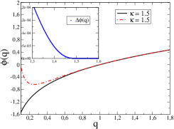
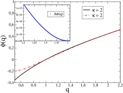
Figure 1: The two branches of the $\phi(q)$ function across the Potts model phase transition for the hidden variables ensembles with average degree distributed according to a Poissonian. The solid line indicate the function $\phi(q)$ calculated at the asymmetric solution of the Potts model and the dot-dashed line indicate the function $\phi(q)$ calculated for the symmetric solution. For $\kappa\leq 2$ the free energy at the phase transition varies continuously, from the $\rho=0$ solution to the asymmetric solution. The inset show the difference of the free energy calculated on the two branches. In the left figures $\kappa=1.5$ while in the right $\kappa=2$.

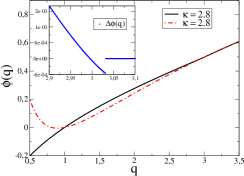
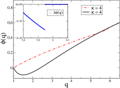
Figure 2: The two branches of the $\phi(q)$ function across the Potts model phase transition for the Configuration model with the average of the degrees at each node distributed according to a Poissonian. The solid line indicate the function $\phi(q)$ calculated at the asymmetric solution of the Potts model and the dot-dashed line indicate the function $\phi(q)$ calculated for the symmetric solution. The free energy at the transition varies discontinuously at $q_{c}\geq\kappa=\langle{\overline{k}}\rangle+1$ when the metastable Configuration $\rho\neq 0$ disappears. The inset shows explicitly the discontinuity in the difference $\Delta\phi$ between the function $\phi$ calculated on the two solutions.

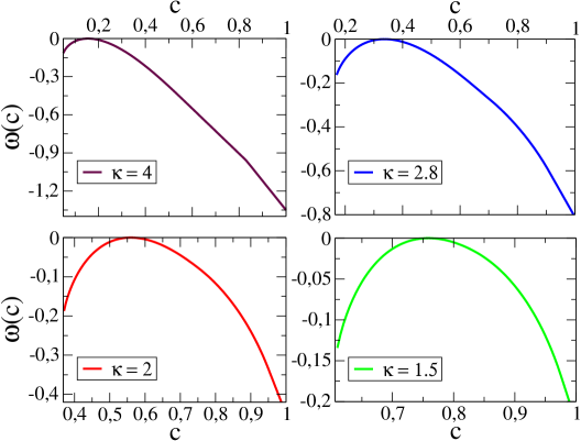
Figure 3: We show the numerically evaluated $\omega(c)$ function for the hidden variable Configuration model in which the average degrees are distributed according to a Poisson distribution with $\kappa=1+\langle{\overline{k}}\rangle$. We show the dependence on the typical number $c^{*}$ as a function of the mean connectivity. The higher is $\kappa$ the smaller the number of expected typical components.

7 Numerical results

In this section we present the study of the large deviation of cluster distribution for different examples of generalized network ensembles.

• The $G(N,p)$ ensemble
  We consider the simple case of a $G(N,p)$ networks ensembles where the average degree of each node $\theta_{i}$ is independent on $i$, i.e. $\theta_{i}=\sqrt{\langle{\overline{k}}\rangle/N}$, i.e. $p=\langle{\overline{k}}\rangle/N$. The equation $(\ref{rhognp})$ is the self-consistent equation for the Potts model phase transition. This equation has been already studied [13] where it was found that the Potts model has phase transition in $q_{c}=\langle{\overline{k}}\rangle$ of second order for value of $q_{C}\leq 2$ and of first order for $q_{c}>2$. We suggest the reader to refer to references [14, 13] for a full account of this case.

• The Configuration model
  In particular we study the limit of weak heterogeneity when we assume that the average degree of the nodes $\{\overline{k}\}$ is Poisson distributed and the case of strong heterogeneity of the degree of the nodes when the hidden variables $\{\theta_{i}\}$ are distributed according to a power-law.

  • Poisson hidden variable distribution
    We consider the case in which the distribution of the mean values for the connectivity’s $\overline{k}_{i}$ is Poisson and $\theta_{i}=\sqrt{\overline{k}_{i}/N}$. This ensemble introduce a small heterogeneity with respect to pure Erdös and Rényi networks. In this case the critical point is equal to $q_{c}=N\langle\theta^{2}\rangle=\langle{\overline{k}}\rangle+1$. Therefore the percolation transition happens at $\langle{\overline{k}}\rangle+1=1$ revealing that the percolating phase is already when the mean connectivity is $\langle{\overline{k}}\rangle\rightarrow 0$.

    As predicted by the theoretical results we found a phase transition for $q_{c}=N\langle{\theta^{2}}\rangle=\langle{\overline{k}}\rangle+1$ depending on the mean value of connectivity $\langle\overline{k}\rangle$. In figures 1 and 2 we show the function $\phi(q)$ as a function of $q$ for different values of the parameter $\kappa=\langle{\overline{k}}\rangle+1$ that has the same role of the inverse temperature in the associated Potts model. The phase transition is of the second order when $q_{c}=\langle\overline{k}\rangle+1\leq 2$ (See figure 1). On the contrary, when $\langle\overline{k}\rangle+1>2$, (See figure 2).

    

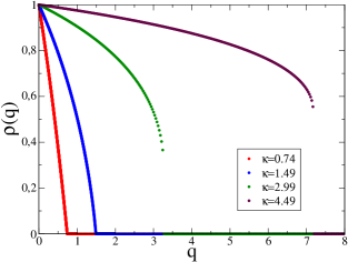
    Figure 4: The solution of the self-consistent equation $(\ref{rhoc})$ for the parameter $\rho$ as a function of the number of colors $q$ for a scale-free random networks with different values of the critical point $q_{c}=\kappa=\langle{\overline{k(k-1)}}\rangle{\langle{\overline{k}}\rangle}$ and power-law exponent $\gamma=5$.

    

    

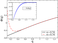
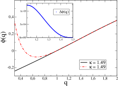
    Figure 5: The two branches of the $\phi(q)$ function for a Configuration model with in power-law distribute $\{\theta\}$’s with exponent $\gamma=5$. The solid line is the function $\phi(q)$ calculated at the asymmetric solution of the Potts model and the dot-dashed line is the function $\phi(q)$ calculated for the symmetric solution. The transition point is at $q_{c}=\kappa=N\langle\theta^{2}\rangle\leq 2$. In the inset we show the difference in free energy in the two branches which is continuous.

    In figure $(\ref{omega})$ we show the function $\omega(c)$ for this ensemble for different values of $\kappa=1+\langle{\overline{k}}\rangle$.We obtain that for value of $c\leq\hat{c}=e^{-\langle{\overline{k}}\rangle}$ the function $\omega(c)$ tends to infinity, i.e $\omega(c)\to-\infty$. This value is relative to the minimum number of components that are equivalent to the number of isolated vertices. Therefore we plot the function $\omega(c)$ only for $c>\hat{c}$. As a function of the parameter $\langle\overline{k}\rangle$ we found that different number of connected components are dominant and in particular for $\langle\overline{k}\rangle+1>2$ we find that the typical number of cluster are lesser that 0.5 and that in the limit of high $\langle{\overline{k}}\rangle$ this number vanishes (See figure 3).

  • Scale-free degree distribution
    We use as degree distribution $p_{\theta}\sim\theta^{-\gamma}$ with $\gamma>3$ so that the second moment does not vanish. We fixed the exponents $\gamma$, letting the value of infrared cutoff changes in order to fix all the moments $\langle\theta^{m}\rangle$. In figure 4 we show the behavior of the solution $\rho$ of the self-consistent equation $(\ref{rhoc})$ as a function of the parameter $q$ for scale-free networks. When $q<q_{c}$ defined by equation $(\ref{qc})$, i.e. $q_{c}=\langle{\overline{k(k-1)}}\rangle/\langle{\overline{k}}\rangle$ a non zero solution $\rho\neq 0$ is found while for $q>q_{c}$ the $\rho=0$ solution becomes the stable one. The value of the stable solution $\rho$ of equation $(\ref{rhoc})$ close to the phase transition $q\simeq q_{c}$ varies continuously in the case $q_{c}\leq 2$ and discontinuously for $q>2$. There is a second order phase transition for values of $\frac{\langle\overline{k(k-1)}\rangle}{\langle\overline{k}\rangle}\leq 2$ and a first order phase transition for $\frac{\langle\overline{k(k-1)}\rangle}{\langle\overline{k}\rangle}>2$ where the free energy discontinuously goes to zero as shown in figure 5.

    In figure 5 and 6 we plot the difference of the $\phi(q)$ functions calculated on the two branches of the solution of $(\ref{rhoc})$ (the solution with $\rho=0$ and the other non trivial solution stable for $q<q_{c}$). From these figures we can see that $\Delta\phi(q)$ has a discontinuity in the regime $\frac{\langle\overline{k(k-1)}\rangle}{\langle\overline{k}\rangle}>2$ and vanishes continuously in the regime $\frac{\langle\overline{k(k-1)}\rangle}{\langle\overline{k}\rangle}\leq 2$.

    

    

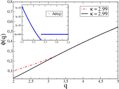
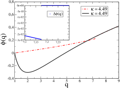
    Figure 6: The two branches of the $\rho(q)$ function for value of parameter $\kappa=N\langle\theta^{2}\rangle>2$ for scale free network $\gamma=5$. In the inset we show the difference between the free energy associated to the symmetric solution $\rho=0$ and the free energy associated to the other asymmetric solution with $\rho\neq 0$. In the figure we report the difference of the free energy calculated on the two branch solution showing evidence for the discontinuity in the free energy at the transition point.

    In figure 7 is shown the probability of large deviation in the number of clusters for the Configuration model with power-law distributed value of $\{\theta\}^{\prime}s$. The typical number of clusters $c^{\star}$ is a decreasing function of $\kappa=\langle{\overline{k(k-1)}}\rangle/\langle{\overline{k}}\rangle$.

    

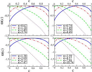
    Figure 7: The logarithm of the probability density function $\omega(c)$ versus the number of connected components $c$. It is easy to identify the typical value $c^{\star}$ when the function $\omega$ touches the zero axis. This number depends strongly on $\kappa=N\langle\theta^{2}\rangle$. Each network correspond to different choice of the parameter $\gamma=7,5,3.5,3.01$ starting from the top on the left.

    

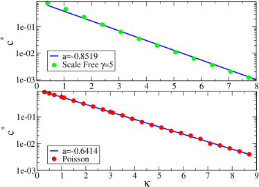
    Figure 8: The typical number of clusters per vertex $c^{\star}$ vanishes exponentially fast with the increasing of $\kappa=N\langle\theta^{2}\rangle$. Here we show in a logarithmic scale this relation for Poissonian degree distribution and power-law networks for value a value of $\gamma=5$. We report also the value from the best fitting calculation that has a good agreement with the data points.

  • Comparison of the typical number of cluster for Configuration model with Poisson and power-law distributed $\{\theta\}$’s.
    The typical value of the number of clusters $c^{\star}$ depends on the parameter $N\langle\theta^{2}\rangle$. This dependencies is shown in figure 8. In the case of power-law distributed $\{\theta\}^{\prime}s$, the characteristic scale above which the number $c^{*}$ vanishes is higher than in Poisson case.

• Simple case of structure network: Network with four equal communities

  

  

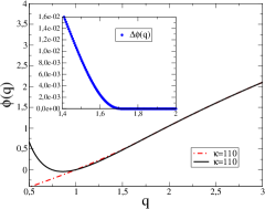
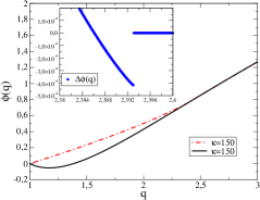
  Figure 9: In figure we plot $\phi(q)$ on the two branches of the solution for network with four communities (second case under study). The network ensemble is characterized by a $W(\alpha,\alpha^{\prime})$ given by (109) with $x=0.5$ and different values of $\theta$, $\theta=110$ and $\theta=150$. This network show the same crossover between a first order and a second order phase transition as soon as the parameter $\theta>\theta_{c}$ calculated in equation 111, $\theta_{c}=120$.The solid line indicate the function $\phi(q)$ calculated at the asymmetric solution of the Potts model and the dot-dashed line indicate the function $\phi(q)$ calculated for the symmetric solution. This is more clear by the discontinuity in the difference of $\phi(q)$ calculated in two branches of the solution reported on the inset. The solid line corresponds to $\rho=0$ while the dashed one is $\phi(q)$ calculated on the non trivial solution $\rho\neq 0$.

  

  Figure 10: We report the logarithm of the cluster probability $\omega(c)$ for the study network ensemble with four communities (second case under study). The network ensemble is characterized by a $W(\alpha,\alpha^{\prime})$ given by (109) with $x=0.5$ and the two different values of $\theta$, $\theta=110$ and $\theta=150$. The distribution is dominated by the typical number $c^{*}$ that depends strongly on the average connectivity of the network ensembles.

  In general the case of structure networks with non trivial $W(\alpha,\alpha^{\prime})$ functions have to be studied on a case by case approach.

  • First case- Here we consider the particular example in which the network is divided in four equivalent communities. This networks have been considered as a benchmark networks with community structure [27]. We consider in particular the case with $N\theta_{i}=\mbox{const}\quad\forall i$ and the network divided in four communities $\alpha=1,2,3,4$, i.e. $A=4$ with

    $$W(\alpha,\alpha^{\prime})=\left\{\begin{array}[]{lcr}\ \frac{x}{64}&\mbox{for }&\alpha=\alpha^{\prime}\\ \frac{(1-x)}{192}&\mbox{for}&\alpha\neq\alpha^{\prime}\end{array}\right.$$ (109)

    In this case we find that for $q>1/64$ the only stable solution is the zero one while for lower value of the parameter $q$ there is a non zero solution that is stable everywhere independently on the value of $x$. We want to emphasize the fact that, substituting equation (109) in (77), we obtain the critical relation reads

    $$q_{c}=\frac{1}{64}\,,$$ (110)

    showing there is no phase transition for every value of the parameter $x$ at fixed $\theta$ and $x$.

  • Second case- We consider the case with four communities $\alpha=1,2,3,4$, i.e. $A=4$ with $W(\alpha,\alpha^{\prime})$ given by $(\ref{interaction})$ at fixed $x$ for the value of the hidden variables $\theta_{i}=\theta\quad\forall i\in A$. The behaviour in that case is exactly the same as in the Configuration model. There is a crossover between first and second order phase transition governed by the parameter $\theta$. The threshold value is given by the relation

    $$\theta_{c}=2(\psi+(A-1)\phi)^{-1}$$ (111)

    and substituting the value of the parameter $x=0.5$ and $A=4$, the critical value is of order $\theta_{c}\sim 120$. The free energy is shown in figure 9 where it is easily to catch the nature of the phase transition. For completeness we report also the logarithm of the clusters distribution in figure 10 that show the same behaviour of Configuration model.

8 Conclusions

In conclusion, we have studied the percolation transition and the large deviation of the cluster distribution in generalized canonical random network ensembles. The calculation has been performed by mapping the problem of finding the cluster distribution on a fully connected Potts model with heterogeneous couplings. The results generalize the known results for uncorrelated configuration models to correlated configuration models and are able to predict the behavior of the phase transition for generic structured networks with non-trivial community or spatial structure. Ongoing work will investigate what is the role of the percolation properties in generalized random network ensembles for the understanding of the critical behavior of dynamical models defined on them and for the characterization of their small loops distribution.

9 Acknowledgments

This paper was supported by the project IST STREP GENNETEC contract No. 034952 and by MIUR grant 2007JHLPEZ.

References

- [1] S.N. Dorogovtsev, A. V. Goltsev, and J. F. F. Mendes. Rev. Mod. Phys., 80:1275, 2008.
- [2] M. Molloy and B. A. Reed. Rand. Struc. Algor. 6:161, 1995.
- [3] R. Albert, H. Jeong, and A.-L. Barabási. Nature, 406:378, 2000.
- [4] R. Cohen, K. Erez, D. ben Avraham, and S. Havlin. Phys. Rev. Lett., 85:4626, 2000.
- [5] R. Cohen, K. Erez, D. ben Avraham, and S. Havlin. Phys. Rev. Lett., 86:3682, 2001.
- [6] S.N. Dorogovtsev, A. V. Goltsev, and J. F. F. Mendes. Phys. Rev. E, 66:016104, 2002.
- [7] M. Leone, A. Vazquez, A. Vespignani, and R. Zecchina. Eur. Phys. J. B, 28:191, 2002.
- [8] G. Bianconi. Phys. Lett. A, 303:166, 2002.
- [9] N. S. Skantzos, I. Pérez Castillo, and J. P. L. Hatchett. Phys. Rev. E, 72:066127, 2005.
- [10] A. C. C. Coolen et al. J. Phys. A: Math. and Gen., 38:8289, 2005.
- [11] J. D. Noh. Eur. Phys. J. B, 66:251, 2008.
- [12] B. B. Bollobas. Random graphs. Cambridge, University Press, 2001, 2nd ed. edition, 1985.
- [13] Engel, Monasson, and Hartmann. J. Stat. Phys., 117(3):387, 2004.
- [14] C. M. Fortuin and P.W. Kasteleyn. Physica, 57:536, 1972.
- [15] M. Boguna and M. A. Serrano. Phys. Rev. E, 72:016106, 2005.
- [16] A. V. Goltsev, S. N. Dorogovtsev, and J. F. F. Mendes. Phys. Rev. E, 78:051105, 2008.
- [17] G. Bianconi. Europhys. Lett., 81:28005, 2008.
- [18] G. Bianconi. http://arXiv:0802.2888, 2008.
- [19] J. Park and M. E. J. Newman. Phys. Rev. E 70: 066146, 2004.
- [20] B. Sodeberg. Phys. Rev. E 66:066121, 2002.
- [21] F. Chung and L. Lu. PNAS 100:6313, 2002.
- [22] G. Caldarelli, A. Capocci, P. De Los Rios and M. A. Muñoz. Phys. Rev. Lett. 85:5468, 2002.
- [23] M. Boguñá and R. Pastor-Satorras. Phys. Rev. E 68:036112, 2003.
- [24] D. S. Lee, K. I. Goh, B. Kahng, and D. Kim. Nuclear Physics B, 696(3):351 – 380, 2004.
- [25] F. Wu. Rev. Mod. Phys., 54:235, 1982.
- [26] T. C. Lubensky. Thermal and geometrical critical phenomena in random systems, in La Matière Mal Condensée Les Houches 1978 ed. R Balian, R Maynard and G Toulouse New York : North-Holland Pub. Co., 1979.
- [27] M. Girvan and M. E. J. Newman. Proc. Natl. Acad. Sci., 99:7821, 2002.