Fakultät für Physik
Universität Karlsruhe (TH)
Diploma thesis
in Physics
submitted by
Julian P. Moosmann
born in Bretten, Germany.
2008

Zusammenfassung

We consider spatial coarse-graining in statistical ensembles of non-selfintersecting and one-fold selfintersecting center-vortex loops as they emerge in the confining phase of SU(2) Yang-Mills thermodynamics. This coarse-graining is due to a noisy environment and described by a curve shrinking flow of center-vortex loops locally embedded in a two-dimensional flat plane. The renormalization-group flow of an effective ‘action’, which is defined in purely geometric terms, is driven by the curve shrinking evolution.

In the case of non-selfintersecting center-vortex loops, we observe critical behavior of the effective ‘action’ as soon as the center-vortex loops vanish from the spectrum of the confining phase due to curve shrinking. This suggest the existence of an asymptotic mass gap.

An entirely unexpected behavior in the ensemble of one-fold selfintersecting center-vortex loops is connected with the spontaneous emergence of order. We speculate that the physics of planar, one-fold selfintersecting center-vortex loops to be relevant for two-dimensional systems exhibiting high-temperature superconductivity.

Zusammenfassung

Die Anregungen der konfinierten Phase in der thermodynamischen Behandlung der SU(2) Yang-Mills Theorie sind Zentrumsvortexschlaufen welche aufgrund der Wechselwirkung mit einer rauschenden Umgebung Schrumpfungsprozess unterliegen. Wir betrachten statistische Ensemble von Zentrumsvortexschlaufen ohne und mit einfachen Schnittpunkt welche in einer flachen zweidimensionalen Ebene lokal eingebettet sind. Der Schrumpfungsprozess von eingebetteten Zentrumsvortexschlaufen wird durch eine Diffusionsgleichung beschrieben. Der Renormierungsgruppenfluss einer in rein geometrischen Größen definierten effektiven „Wirkung“ wird durch die Evolution schrumpfender Kurven bestimmt.

Im Falle von Zentrumsvortexschlaufen ohne Schnittpunkt beobachten wir ein kritisches Verhalten der effektiven „Wirkung“ sowie die Vortexschlaufen aufgrund des Schrumpfungsprozesses aus dem Spektrum der konfinierten Phase verschwinden. Dies legt die Existenz eines asymptotischen Massen-Gaps nahe.

Ein vollkommen unerwartetes Verhalten im Ensemble von Zentrumsvortexschlaufen mit einfachem Schnittpunkt steht in engem Zusammenhang mit dem spontanen Auftreten von Ordnung. Wir vermuten, dass die Physik ebener Zentrumsvortexschlaufen relevant ist für die Beschreibung zweidimensionaler Systeme, welche die Eigenschaft der Hochtemperatursupraleitung aufweisen.

Solitonic fermions
in the confining phase
of SU(2) Yang-Mills theory This diploma thesis has been carried out by
Julian P. Moosmann
at the
Institut für Theoretische Physik
under the supervision of
Priv.-Doz. Dr. Ralf Hofmann

Chapter 1 Introduction

The importance of Yang-Mills theories in mathematical and theoretical physics is generally acknowledged. Yang-Mills gauge theories are the cornerstone of quantum field theories in the Standard Model of Particle Physics: Besides gravity, all fundamental interactions are incorporated as gauge symmetries in the Standard Model. Although it has been examined in the framework of perturbation theory due to the enormous complexity implied in the full story of (especially non-Abelian) gauge theories, the Standard Model has produced a lot of striking results and predictions. There are many examples, such as the explanation of the anomalous magnetic moment of the electron, the feature of asymptotic freedom of Quantum Chromodynamics in the high energy limit, or the prediction of flavor-changing neutral currents in electroweak processes [1]. However, there are still a number of unsolved mathematical problems and unexplained experimental observations. Among those are: The necessity of an asymptotic mass gap and a rigorous proof of color confinement in pure Yang-Mills theory [2]. In the Standard Model, the assumption of a zero rest mass of the neutrino is refuted by the observation of neutrino oscillations [3] and the double $\beta$ decay [4]. These observations indicate a small, finite rest mass that also cannot be excluded by recent experiments measuring the spectrum of the single $\beta$ decay of tritium nuclei near the endpoint [5, 6]. Furthermore, the Standard Model does not provide for an explanation of Dark Matter and Dark Energy that account for about 96% of the energy density in the present universe, and the predicted Higgs particle has evaded experimental detection so far. Moreover, the perturbation series of four-dimensional quantum field theories is most likely an asymptotic series; the fact that a perturbative calculation of the thermodynamical pressure cannot be driven beyond order $g^{5}$ in the coupling constant due to the weak screening of the magnetic sector causing infrared instabilities [7], could be shown for Quantum Chromodynamics at finite temperature.

Since perturbation theory is an expansion in powers of a necessarily small coupling constant about a trivial a priori estimate for the vacuum of the theory, it fails to describe strongly coupled physics as well as the according nontrivial vacuum state. This vacuum is certainly composed of finite-action solitonic solutions of the classical Yang-Mills action. The so called instantons are topologically nontrivial objects in pure Yang-Mills theory that describe tunneling processes between topological distinct vacua, e.g. [8]. Their weight possesses an essential zero at vanishing coupling, and thus instanton contributions to the partition function of the theory are completely ignored by perturbation theory. Instantons at finite temperature are called calorons.

Therefore, we are advised to consider a nonperturbative approach to gauge theories. Such a treatment has already been proven successful in terms of an effective theory for superconductivity [9]. An analytical and nonperturbative approach to SU(2) Yang-Mills thermodynamics was developed in [10]. In this approach the basic idea is to subject the highly complex dynamics of the topologically nontrivial field configurations to a spatial coarse graining that leads to the emergence of macroscopic scalar fields, and pure gauges. Due to nontrivial (thermal) ground states, the fundamental gauge symmetry is broken successively as temperature decreases. As a consequence, Yang-Mills thermodynamics occurs in three phases: the deconfining, the preconfining and the confining phase. The latter, in which we are primarily interested in this thesis, exhibits three unexpected results. These are the exact vanishing of the energy density and the pressure of the ground state at zero temperature, the Hagedorn character of the preconfining-confining phase transition and the spin-1/2 nature of the massless and massive excitations in the confining phase.

The ground state of the deconfining phase is composed of interacting calorons and anticalorons and exhibits negative pressure. The propagating excitations within that phase are two massive gauge modes - due to the dynamically broken SU(2) - and one massless gauge mode. As temperature decreases, the likeliness for calorons and anticalorons to dissociate into (BPS saturated) magnetic monopoles and antimonopoles increases strongly in the vicinity of a critical temperature. The ground state of the preconfining (or magnetic) phase starts to form by the pairwise condensation of monopoles and antimonopoles. Excitations in that phase are propagating dual gauge modes of mass $m_{\scriptscriptstyle D}$ (dynamically broken U(1)_D). Unstable defects of the magnetic ground state are closed magnetic flux lines of finite core size $d$ that collapse as soon as they are created. This is because, as long as $d>0$, the pressure inside the vortex loop is more negative than outside, thus leading to the contraction of the vortex loop. The magnetic phase exhibits negative pressure. At the Hagedorn transition towards the confining (also called center) phase, a complete decoupling of the gauge fields takes place. To put it more precisely, by the decay of the magnetic ground state into selfintersecting and non-selfintersecting center-vortex loops the mass of the dual gauge field diverges and the core size of center-vortex loops vanishes, see also [11, 12]. As a result of $d\rightarrow 0$, the negative pressure $P$ is confined to the vanishing vortex core. This implies that center-vortex loops become stable particle-like excitations with $P=0$. These solitons are classified according to their center charge and the number of selfintersections $N$, see Fig. 1.1. The mass of an $N$-fold selfintersecting soliton is $N\Lambda_{C}$, where $\Lambda_{C}$ is the Yang-Mills scale. Topologically, solitons with non-vanishing $N$ are stable in the absence of external gauge modes coupling to the charges at the intersection points. On the other hand, for $N=0$, there is no topological reason for stability.

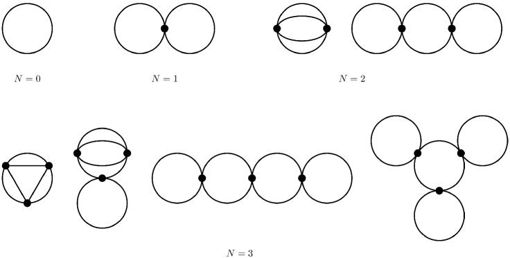
Figure 1.1: The topologies of solitonic excitations with up to $N=3$ selfintersections for an SU(2) Yang-Mills theory in the confining phase. A magnetic monopole of charge $+1$ or $-1$ is located at each point where center-flux lines intersect. Solitons with $N=0$ are unstable in presence of a noisy environment, whereas solitons with $N=1$ are always stable. Excitations with $N>1$ are unstable if subjected to mixing with theories possessing propagating gauge fields.

Now consider a situation where a planar center-vortex loop, which is a (local) embedding of a center-vortex loop into a two-dimensional flat and spatial plane, still has non-vanishing core size $d>0$ and the mass of the dual gauge field $m_{\scriptscriptstyle D}$ is still finite due to a noisy environment which locally resolves the otherwise infinitely thin vortex. In this case, the pressure $P$ is locally nonzero and the soliton starts shrinking. Such a situation is described by a curve shortening flow in the (dimensionless) parameter $\tau$. Here, $\tau$ is a variable measuring the decrease of externally provided resolving power applied to the system. There is a functional dependence of $\tau$ on the corresponding resolution $Q$ (momentum transfer). For an isolated SU(2) theory the role of the environment is played by the sectors with $N>0$. If the confining SU(2) is part of a world with additional gauge symmetries, then a portion of such an environment arises from the mixing between the corresponding gauge groups. Either way, a center-vortex loop acquires a finite core size and as a consequence, a finite mass for the $N=0$ soliton by frequent interaction with the environment after it was generated by a process that was subject to an inherent, finite resolution $Q_{0}$.

Knot-like structures are relevant in a number of chemical, biological and physical systems [13], e.g. in polymer physics, particularly in molecular biology, in type-II superconductor, where string-like vortices confine magnetic fields to the cores of the vortex-like structures, in superfluid helium (${}^{4}\mathrm{He}$), as well as in liquid crystals. As early as 1897 Lord Kelvin proposed that elementary particles - at that time atoms were considered to be elementary by Kelvin and others - should be described as knotted lines of vortex tubes in a medium (the aether) [14]. As we know now, the point particle interpretation of Quantum Mechanics appears to be a much more elegant and efficient framework to describe the physics of atoms and molecules. But at the same time, the notion of an electron as a spinning point particle, albeit an excellent description in a bulk of physical situations in atoms, colliders and condensed matter systems, causes theoretical and experimental inconsistencies. On the one hand, there is the problem of diverging classical self-energy of the electron. On the other hand, the unexpected explosive behavior in recent high-temperature plasma experiments [15, 16] and the strong correlations of electrons in two-dimensional planar systems [9] are indications of non-local effects possibly related to the extended spatial structure of the electron. Also, recent theoretical developments revive Kelvin’s description of elementary particles as non-local knot-like entities. In [13, 17], the argument is that confining strings, tied into stable knotted solitons, exist when decomposing the gauge field in the low-energy domain of four-dimensional SU(2) Yang-Mills theory.

According to the approach in [10], we tend to interpret one-fold selfintersecting center-vortex loops as electrons and accordingly non-selfintersecting center-vortex loops as neutrinos. This implies that the Yang-Mills scale $\Lambda_{C}$ must be set equal to the electron mass $m_{e}=511$ keV. The spin-1/2 nature of a center-vortex loop is a consequence of its two-fold degeneracy with respect to the direction of flux which is lifted in the presence of an electric or magnetic background field. It should be noticed for a selfintersecting center-vortex loop that, as long as both wings of center flux are of finite size, a spatial shift of the intersection point requires a negligible amount of energy only. In particular, if the inner angle $\alpha$ between in- and out-going center-flux at the intersection is sufficiently small, then a motion of points on the vortex line that is directed perpendicularly to the bisecting line of the angle $\alpha$ easily generates a velocity of the intersection point which exceeds the speed of light, e.g. Fig. 1.2. Here, it should be considered that the path-integral formulation of Quantum Mechanics admits such superluminal motion in the sense that the according trajectories contribute to transition amplitudes [18].

Figure 1.2: Points on the center flux lines moving oppositely on a line perpendicular to the bisecting line of the angle $\alpha$ with velocity modulus $v_{1}$. For sufficiently small $\alpha$ the velocity modulus $v_{2}$ of the intersection point is superluminal: $v_{2}=v_{1}\cot{\frac{\alpha}{2}}$.

The purpose of this thesis is to treat the behavior of $N=0$ and $N=1$ center-vortex loops under curve shrinking as a Wilsonian renormalization-group flow governed by an effective ‘action’. The term ‘action’ is slightly misleading since we do not aim at a time evolution of the system by demanding stationarity of the ‘action’ under curve variation. We consider resolution dependent statistical ensembles in the presence of an environment represented by a parameter $\sigma$. The corresponding weight-functional for the members of the ensemble, written as the exponential of an ‘action’, is defined in purely geometric terms. In turn the resolution dependence of the ‘action’ is determined by the curve shrinking flow. The ‘action’ possesses a natural decomposition into a conformal and a non-conformal factor. We consider the partition function of a given ensemble of planar curves to be invariant under the condition of changing the resolution. Once the evolution of the weight-functional is determined, we are able to compute the resolution dependence of ‘observables’ as ensemble averages of (local or non-local) operators.

What we observe is that the $N=0$ sector becomes unresolvable from a finite resolution $Q_{*}$ downward. That is, as a consequence of a noisy environment planar $N=0$ center-vortex loops shrink to points with circular limiting shape within a finite decrease of resolving power and thus disappear from the spectrum of the confining phase of SU(2) Yang-Mills theory for a resolution smaller than the critical $Q_{*}$. Since center-vortex loops with $N>0$ have finite mass this generates an asymptotic mass gap. We show that the observed transition to the conformal limit of vanishing curve length is a critical phenomenon with a mean-field exponent of the coefficient associated with the non-conformal factor. For the $N=1$ sector we observe the unexpected behavior that, starting from a finite value, the entropy of the system decreases to an almost zero value as the resolving power is lowered: the ensemble evolves into a highly ordered state in a sense that only a single curve survives the process of coarse-graining.

The thesis is organized as follows: Chapter 2 gives a brief outline of the effective theory of thermalized SU(2) Yang-Mills dynamics in all of its phases as it is developed in [10]. Chapter 3 provides prerequisites for the mathematics of curve shrinking flows in two and three space dimensions. Chapters 4 and 5 investigate the $N=0$ sector and respectively, the $N=1$ sector. In Sections 4.1 and 5.1, we explain our philosophy underlying the statistics of geometric fluctuations and how the renormalization-group flow of the effective ‘action’ is driven by the curve-shrinking evolution of the members of a given ensemble of $N=0$ and respectively, $N=1$ center-vortex loops. In Sec. 4.2, we explain our numerical analysis concerning the computation of the effective action and the variance of the ‘center of mass’ which is compared to Heisenberg’s uncertainty relation. In Sec. 5.2, we elucidate our numerical analysis concerning the computation of the effective ‘action’, the variance of the location of the selfintersection, and the resolution-dependent entropy associated with a given ensemble. Chapter 6 deals with electrons which are interpreted as center-vortex loops with one selfintersection. In Sec. 6.1, we give reasons for this interpretation, and in Sec. 6.2, we consider strongly correlated systems of electrons in cuprates exhibiting high-temperature superconductivity and the new class of recently discovered iron-based high-temperature superconductors. Chapter 7 gives a short summary of our findings.

Chapter 2 Brief review of SU(2) Yang-Mills thermodynamics

In this section, we give a short outline of the analytical and nonperturbative approach to SU(2) Yang-Mills thermodynamics as it is developed in [10]. The basic idea is to subject the highly complex dynamics of topologically nontrivial field configurations to a spatial coarse-graining that is described by emergent macroscopic scalar fields, one for each phase. Conceptually, this approach is similar to the macroscopic Landau-Ginzburg theory of superconductivity. Although we are only concerned with the confining phase in this work, we start our outline of [10] in the deconfining phase at high temperatures which leads us by consecutive phase transitions to the confining phase.

2.1 Basics of thermal Yang-Mills theory

Yang-Mills theories are non-Abelian gauge theories whose Lagrangian is demanded to be invariant under local gauge transformations. In this thesis, we restrict ourselves to the case of SU(2) gauge transformations. In pure Yang-Mills theory, only gauge field terms appear in the fundamental Lagrangian while matter fields are absent. Wick-rotating to Euclidean signature by $t\rightarrow-\mathrm{i}\tau$ and moving to finite temperature $T$, which corresponds to imaginary time compactified on a circle with circumstance $\beta=\frac{1}{T}$, the gauge-invariant action is given by

$$S\equiv\frac{1}{2g^{2}}\mathrm{tr}\int_{0}^{\beta}\mathrm{d}\tau\int\mathrm{d}^{3}x\,F_{\mu\nu}F_{\mu\nu},$$ (2.1)

where $g$ denotes the dimensionless coupling constant and $\mathrm{tr}$ the trace operation. It holds that $(x_{1},x_{2},x_{3},x_{4})\in\mathbb{R}^{4}$. The Yang-Mills field strength tensor is defined as

$$F_{{\mu\nu}}=\partial_{\mu}A_{\nu}-\partial_{\nu}A_{\mu}-\mathrm{i}[A_{\mu},A_{\nu}],$$ (2.2)

with the Lie-algebra valued gauge fields in the adjoint representation

$$A_{\mu}\equiv A_{\mu}^{a}\frac{\sigma^{a}}{2},$$ (2.3)

where the generators $\sigma^{a}$ are given by the Pauli matrices. The action density $\frac{1}{2g^{2}}\mathrm{tr}\,F_{{\mu\nu}}F_{{\mu\nu}}$ is invariant under local SU(2) gauge transformations

$$A_{\mu}(x)\overset{\Omega}{\rightarrow}\Omega(x)A_{\mu}(x)\Omega^{\dagger}(x)+i\Omega(x)\partial_{\mu}\Omega(x),$$ (2.4)

where $\Omega$ is an element of $SU(2)$.

Instantons are localized finite-action classical solutions in Euclidean field theory. The BPST (Belavin-Polyakov-Schwartz-Tyupkin) instanton is an (anti)selfdual, that is BPS (Bogomol’nyi-Prasad-Sommerfield) saturated, configuration solving the Euler-Lagrange equations $D_{\mu}F_{\mu\nu}=0$ subject to the action (2.1) [19]. For the covariant derivative $D_{\mu}$ of the field $\phi$ in the adjoint representation we have

$$D_{\mu}\phi=\partial_{\mu}\phi-\mathrm{i}[A_{\mu},\phi].$$ (2.5)

The (anti)selfduality condition reads

$$F_{\mu\nu}=\pm\tilde{F}_{\mu\nu},$$ (2.6)

where the dual field strength is defined as $\tilde{F}_{\mu\nu}\equiv\frac{1}{2}\epsilon_{\mu\nu\kappa\lambda}F_{\kappa\lambda}$, $\epsilon_{\mu\nu\kappa\lambda}$ being the total antisymmetric tensor with $\epsilon_{1234}=1$. (Anti)selfdual configurations saturate the BPS bound on the action which therefore is minimal (in a given topological sector) and of value

$$S=\frac{8\pi^{2}}{g^{2}}|Q|,$$ (2.7)

where the Pontryagin index $Q$ is a topological invariant (charge) and defined as

$$Q\equiv\frac{1}{32\pi^{2}}\int_{0}^{\beta}\mathrm{d}\tau\int\mathrm{d}^{3}x\,F_{{\mu\nu}}^{a}\tilde{F}_{{\mu\nu}}^{a}.$$ (2.8)

BPS saturated field configurations $A_{\mu}$ have vanishing energy-momentum tensor.

(Anti)calorons are BPS saturated, periodic-in-$\tau$ configurations at finite temperature with finite action and topological charge $Q=\pm 1$. They are classified according to the eigenvalues of their Polyakov loop (time-like Wilson loop evaluated in periodic gauge) at spatial infinity. An (anti)caloron is said to be of trivial holonomy, if its Polyakov loop, evaluated at spatial infinity, is an element of the center of the gauge group. Otherwise it is said to have nontrivial holonomy. The Harrington-Shepard (HS) (anti)caloron is a periodic-in-$\tau$ instanton in singular gauge with topological charge $Q=\pm 1$ and trivial holonomy, whereas the Lee-Lu-Kraan-van Baal (LLKvB) (anti)caloron is of nontrivial holonomy. Descriptively, trivial holonomy means that the caloron has no substructure. The LLKvB (anti)caloron contains BPS magnetic monopoles constituents which, by virtue of quantum corrections [20], are subject to an attractive interaction in the case of small holonomy and to a repulsive interaction for large holonomy. In the case of large holonomy, the repulsion leads to a dissociation of the caloron into a pair of a screened magnetic monopole and antimonopole. On the other hand, for small holonomy, the (anti)caloron collapses back to the stable configuration of a HS (anti)caloron by annihilation of their BPS monopole constituents. Thus, single LLKvB calorons are unstable under quantum deformations.

2.2 The deconfining phase

The complex microscopic dynamics in Yang-Mills theory does not seem to allow for a direct analytic calculation of macroscopic quantities in terms of the fundamental gauge fields. A spatial coarse-graining, that is the computation of a spatial average over the sector of topologically nontrivial, BPS saturated field configurations of trivial holonomy turns out to be a feasible and thermodynamically exhaustive approach. The coarse-graining procedure is described in terms of a macroscopic adjoint field $\phi$. In order to characterize the macroscopic ground state, $\phi$ has to satisfy for following conditions:

(i) due to spatial isotropy and homogeneity $\phi$ must be a Lorentz scalar;

(ii) homogeneity of the ground state implies that the modulus of $\phi$ is independent of space and time. A dynamically generated Yang-Mills scale $\Lambda$ enters this modulus as a parameter;

(iii) $\phi$ is a composite of local fields and therefore has to transform under the adjoint representation, because in pure Yang-Mills theory all local fields transform under the adjoint representation of the gauge group;

(iv) only the color orientation of $\phi$ in a given gauge, also referred to $\phi$’s phase, depends on $\tau$. Since $\phi$ is constructed from (anti)calorons, which are periodic in Euclidean time, $\phi$’s phase is also periodic in $\tau$, and since the classical caloron action $S=\frac{8\pi}{g^{2}}$ is independent of temperature $\phi$’s phase is not explicitly time dependent. The computation of the phase of $\phi$ does not require any information about the Yang-Mills scale.

Consequently, the field can be written as

$$\phi^{a}=|\phi|(\Lambda_{E},\beta)\frac{\phi^{a}}{|\phi|}\left(\frac{\tau}{\beta}\right).$$ (2.9)

In [10, 21, 22] equations of motion for the phase and modulus of the spatially homogeneous, composite, emergent adjoint scalar field $\phi$ obeying the above conditions are derived. The (non-perturbatively) temperature dependent modulus is given by

$$|\phi|(\Lambda_{E},\beta)=\sqrt{\frac{\Lambda_{E}^{3}\beta}{2\pi}}=\sqrt{\frac{\Lambda_{E}^{3}}{2\pi T}}.$$ (2.10)

The corresponding action is found to be

$$S_{\phi}=\mathrm{tr}\int_{0}^{\beta}\mathrm{d}\tau\int\mathrm{d}^{3}x\;((\partial_{\tau}\phi)^{2}+\Lambda_{E}^{6}\phi^{-2}),$$ (2.11)

where $\phi^{-1}\equiv\frac{\phi}{|\phi|^{2}}$. The field $\phi$ turns out to be quantum mechanically and statistically inert. It serves as a spatially homogeneous background for the topologically trivial ($Q=0$) sector of the coarse-grained, propagating gauge fields $a_{\mu}$. In Eq. (2.11) interactions between calorons are not yet included. This is done via minimal coupling by substituting

$$\partial_{\mu}\phi\rightarrow D_{\mu}\phi=\partial_{\mu}\phi+\mathrm{i}e[\phi,a_{\mu}].$$ (2.12)

The interactions are mediated by the topologically trivial fields that change the holonomy of the (anti)calorons and subsequently induce interactions between the magnetic monopole constituents of nontrivial holonomy (anti)calorons. The action for the minimally coupled fields is given by

$$S=\mathrm{tr}\int_{0}^{\beta}\mathrm{d}\tau\int\mathrm{d}^{3}x\;(\frac{1}{2}G_{\mu\nu}\,G_{\mu\nu}+(D_{\mu}\phi)^{2}+\Lambda^{6}\phi^{-2}),$$ (2.13)

where the field strength is $G_{\mu\nu}\equiv\frac{\sigma^{a}}{2}(\partial_{\mu}a_{\nu}^{a}-\partial_{\nu}a_{\mu}^{a}-ef^{abc}a_{\mu}^{b}a_{\nu}^{c})$ and $e$ denotes the effective gauge coupling which determines the strength of interaction between topologically trivial gauge field fluctuations and the macroscopic field $\phi$. Due to Lorentz invariance, gauge invariance, perturbative renormalization, and the inertness of $\phi$ the action (2.13) is unique. The topologically trivial sector is written as a decomposition

$$a_{\mu}=a_{\mu}^{gs}+\delta a_{\mu},$$ (2.14)

where $a_{\mu}^{gs}$ is a pure-gauge solution of the equations of motion for $a_{\mu}$ following from action (2.13), and $\delta a_{\mu}$ is a (periodic) finite-curvature propagating fluctuation. The pressure $P^{gs}_{E}$ and energy density $\rho^{gs}_{E}$ of the ground state, following from the energy-momentum tensor, read

$$P^{gs}_{E}=-\rho^{gs}_{E}=-4\pi\Lambda_{E}^{3}T.$$ (2.15)

Microscopically, the negative ground state pressure arises from the creation and annihilation of BPS monopoles and antimonopoles within small-holonomy (anti)calorons. The emergence of the macroscopic adjoint scalar field $\phi$ breaks the fundamental gauge group SU(2) down dynamically to the subgroup U(1). Due to the adjoint Higgs mechanism, two out of three gauge modes $\delta a_{\mu}^{(1,2)}$ acquire a temperature dependent mass, while the third remains massless,

$$m_{1}=m_{2}=2e(T)|\phi|=2e(T)\sqrt{\frac{\Lambda_{E}^{3}}{2\pi T}}\qquad\textnormal{and}\qquad m_{3}=0.$$ (2.16)

Evaluating the Polyakov loop in a different (unitary) gauge gives rise to the conclusion that the ground state is two-fold degenerated with respect to the (broken) global electric $Z_{2}$ symmetry. Thus, the electric phase is deconfining. The temperature evolution of the effective gauge coupling $e$ is derived from the demand for thermodynamical self-consistency, it reaches a plateau value rapidly as temperature increases ($T\gg T_{c,E}$) and diverges logarithmically for $T\searrow T_{c,E}$,

$$e(T)\propto-\log(T-T_{c,E}).$$ (2.17)

Figure 2.1: Temperature evolution of the effective gauge couplings $e$ and $g$ as a function of the dimensionless temperature $\lambda_{E}=\frac{2\pi T}{\Lambda_{E}}$. The figure is taken from [23].

Therefore, the massive gauge $\delta a_{\mu}^{(1,2)}$ modes become infinitely heavy and decouple at $T_{c,E}$.

The ground state in the deconfining phase is composed of interacting calorons and anticalorons of topological charge-modulus one and trivial holonomy. Screened magnetic BPS saturated monopoles are spatially isolated defects in the electric phase. Screening occurs due to short-lived magnetic dipoles provided by intermediary small-holonomy LLKvB (anti)calorons and due to all other stable and screened (anti)monopoles.

2.3 The preconfining phase

At $T_{c,E}=13.87\frac{\Lambda_{E}}{2\pi}$, the effective gauge coupling $e$ diverges. Thereby, magnetic monopoles and antimonopoles, which are generated by the dissociation of large-holonomy calorons, become massless and condense pairwise, thus terminating the deconfining phase. Note that for $T<T_{c,E}$, the average caloron-anticaloron holonomy gradually increases with decreasing temperature. After a spatial coarse-graining, the thermal ground state of the Bose condensate of interacting monopoles and antimonopoles is entirely described by a macroscopic complex scalar field $\varphi$ and a pure gauge $a_{\mu}^{\scriptscriptstyle{D},gs}$; only gauge fields transforming under U(1) survive the electric-magnetic phase transition. The macroscopic complex scalar field $\varphi$ turns out to be quantum mechanically and statistically inert. Interactions between monopoles mediated by pure gauges generate isolated but unstable defects. These defects are closed magnetic flux lines that are composed of magnetic monopoles moving oppositely directed to each other in the vortex core along the flux lines. The closed flux lines collapse as soon as they are created, thereby inducing a negative pressure. It should be noticed that the magnetic flux lines need to be closed due to the absence of isolated magnetic charges in the monopole condensate. The spatially homogeneous and BPS saturated complex scalar field $\varphi$ breaks the dual gauge symmetry $\mathrm{U(1)}_{D}$ dynamically: the stable and propagating excitations in the magnetic phase are massive dual gauge modes.

In [10] equations for phase and modulus of the macroscopic complex scalar field are derived. The modulus of the field $\varphi$ is found to be

$$|\varphi|(\Lambda_{M},\beta)=\sqrt{\frac{\Lambda_{M}^{3}\beta}{2\pi}}=\sqrt{\frac{\Lambda_{M}^{3}}{2\pi T}}.$$ (2.18)

The effective action for $\varphi$ reads

$$S_{\varphi}=\int_{0}^{\beta}\mathrm{d}\tau\int\mathrm{d}^{3}x\;\left(\frac{1}{2}\,\overline{\partial_{\tau}\varphi}\,\partial_{\tau}\varphi+\frac{1}{2}\frac{\Lambda_{M}^{6}}{\bar{\varphi}\varphi}\right),$$ (2.19)

where interactions between (screened) monopoles are absent and $\Lambda_{M}$ is an externally provided Yang-Mills scale. Interactions are accounted for in analogy to Sec. 2.2: the topologically trivial sector $a_{\mu}^{\scriptscriptstyle D}$ is decomposed into

$$a_{\mu}^{\scriptscriptstyle D}=a_{\mu}^{\scriptscriptstyle{D},gs}+\delta a_{\mu}^{\scriptscriptstyle D}$$ (2.20)

and is minimally coupled to $\varphi$. The unique effective action including interaction reads

$$S=\int_{0}^{\beta}\mathrm{d}\tau\int\mathrm{d}^{3}x\;\left(\frac{1}{4}F^{\scriptscriptstyle D}_{\mu\nu}\,F^{\scriptscriptstyle D}_{\mu\nu}+\frac{1}{2}\overline{\mathcal{D}_{\mu}\varphi}\,\mathcal{D}_{\mu}\varphi+\frac{1}{2}\frac{\Lambda_{M}^{6}}{\bar{\varphi}\varphi}\right),$$ (2.21)

where the Abelian field strength of the dual gauge field is given by

$$F_{\mu\nu}^{\scriptscriptstyle D}=(\partial_{\mu}a^{\scriptscriptstyle D}_{\nu}-\partial_{\nu}a^{\scriptscriptstyle D}_{\mu}),$$ (2.22)

and the covariant derivative involving the effective magnetic coupling $g$ by

$$\mathcal{D}_{\mu}=\partial_{\mu}+\mathrm{i}ga_{\mu}^{\scriptscriptstyle D}.$$ (2.23)

A pure-gauge solution $a_{\mu}^{\scriptscriptstyle{D},gs}$ to the equations of motions for the dual gauge-field in the background of $\varphi$ is found.

The evaluation of the Polyakov loop suggests that the electric $Z_{2}$ degeneracy, as occurred in the electric phase, no longer exists in the magnetic phase: the ground state of the magnetic phase is unique and confines fundamental, heavy and fermionic test charges. Nevertheless, massive gauge modes still propagate because the Polyakov loop does not vanish entirely. Therefore, the magnetic phase is called preconfining. The dual gauge group U(1)_D is dynamically broken due to the emergence of the macroscopic scalar field $\varphi$. As a consequence, the dual gauge excitation $\delta a_{\mu}^{\scriptscriptstyle D}$ becomes Meißner massive via the dual Abelian Higgs mechanism,

$$m_{\scriptscriptstyle D}=g(T)\varphi.$$ (2.24)

The evolution of the temperature dependent effective gauge coupling $g$ is predicted by thermodynamical self-consistency. The coupling vanishes for $T\nearrow T_{c,E}$ and diverges logarithmically for $T\searrow T_{c,M}$:

$$g\propto-\log(T-T_{c,M}),$$ (2.25)

where $T_{c,M}$ denotes the temperature where the transition to the center phase takes place. The typical energy of a non-selfintersecting center-vortex loop (CVL) is $\propto\;g^{-1}$.

During the electric-magnetic phase transition, the number of polarizations of the ‘photon’ jumps from two to three, thereby inducing a discontinuity in the energy density. The negative pressure of the ground state arises due to an equilibrium between vortex-loop creation by dissociation of large-holonomy calorons and the annihilation of vortex loops by contraction. The non-vanishing pressure $P^{gs}_{M}$ and energy density $\rho^{gs}_{M}$ of the ground state evaluate as

$$P^{gs}_{M}=-\rho^{gs}_{M}=-\pi\Lambda_{M}^{3}T.$$ (2.26)

Across the electric-magnetic phase transition at $T_{c,E}$, where $e=\infty$ and $g=0$, the pressure is continuous (see Fig. 2.2) relating the scales $\Lambda_{E}$ and $\Lambda_{M}$:

$$\Lambda_{E}=\left(\frac{1}{4}\right)^{1/3}\Lambda_{M}.$$ (2.27)

Figure 2.2: Ratio of the energy density $\rho$ and temperature $T^{4}$ across the electric-magnetic phase transition as a function of the dimensionless temperature $\lambda_{E}=\frac{2\pi T}{\Lambda_{E}}$. The dashed line represents the continuation of the energy $\rho_{E}$ of the electric phase (solid black line) for decreasing temperature $T<T_{c,E}$ (supercooled state, $m_{\scriptscriptstyle D}=0$). The solid grey line represents the energy density $\rho_{M}$ in the magnetic phase for increasing temperature ($m_{\scriptscriptstyle D}>0$). As long as no additional energy is available, the system remains in a supercooled state until a temperature $\lambda_{E}=12.15$ is reached. The figure is taken from [23].

The magnetic phase is not detected by finite-size lattice simulations, since the monopoles condensate posses infinite correlation length ($\propto(M_{m+a})^{-1}$), where $M_{m+a}$ is the sum of the monopole and antimonopole mass after screening:

$$M_{m+a}=\frac{8\pi}{e\beta}.$$ (2.28)

2.4 The confining phase

First we provide some facts on the Abrikosov-Nielsen-Olesen (ANO) vortex. When embedded in three space dimensions, a point-like two-dimensional ANO vortex becomes a vortex line. A mesoscopic description of a static ANO vortex is given by the action of Eq. (2.21) where the potential is absent. A BPS saturated solution to the equation of motions, following from action (2.21), can be found that carries one unit of magnetic flux ($\frac{2\pi}{g}$) and has vanishing core size. Outside the vortex core the pressure $P_{v}(r)$, which is isotropic in the $x_{1}\text{-}x_{2}$ plane, reads

$$P_{v}(r)=-\frac{1}{2}\frac{\Lambda_{M}^{3}\beta}{2\pi}\frac{1}{g^{2}}{r^{2}},\qquad(r>0),$$ (2.29)

where $r$ is the radial vector in the $x_{1}\text{-}x_{2}$ plane. Notice the minus sign on the right hand side of Eq. (2.29). For a finite energy, the length of the ANO vortex line must be finite. The configuration is static as long as it possesses cylindric symmetry, but as soon as the vortex is bend the configuration becomes unstable: the pressure inside the vortex loop is more negative than outside. Thus, the vortex collapses as soon as it is created at finite coupling $g$. Notice that in the limit where $g$ diverges the pressure vanishes. This implies that the formerly unstable vortex loop becomes a stable and massless particle-like excitation for temperatures below $T_{c,M}$. The typical core size $d$ and energy $E_{v}$ of a CVL are given by

$$d\propto\frac{1}{m_{\scriptscriptstyle D}}=\frac{1}{g}\sqrt{\frac{\Lambda_{M}^{3}}{\beta}}\qquad\textnormal{and}\qquad E_{v}\propto\frac{\pi}{g}\sqrt{\frac{\Lambda_{M}^{3}\beta}{2\pi}}.$$ (2.30)

By the collective dissociation of large-holonomy calorons and anticalorons in the preconfining phase, isolated and closed magnetic flux lines start to form. At $T_{c,M}$, where the magnetic coupling $g$ diverges logarithmically, the dual gauge field becomes infinitely heavy. Thus, a complete decoupling of the dual gauge modes takes place at the magnetic-center phase transition. As a result, only contact interactions between center-vortex-loops are possible.

The decay of the monopole-antimonopole condensate and the subsequent formation of the (Bose)condensate of CVLs is described by a macroscopic complex scalar field $\Phi$ in a potential $V_{C}(\Phi)$. The expectation of $\Phi$ is proportional to the expectation of the ’t Hooft loop operator which is a dual order parameter for confinement. CVLs in the magnetic phase are created by phase jumps of $\Phi$ and an increase in the modulus of $\Phi$. This process continues until $\Phi$ relaxes to one of the $Z_{2}$ degenerated, energy and pressure free minima of a potential $V_{C}$. The phase of $\Phi$ is given by a line integral of the dual gauge field $a_{\mu}^{\scriptscriptstyle D}$ along a spatial circle of infinite radius $S^{R=\infty}_{1}$ measuring the (quantized) magnetic flux through the minimal surface $\mathcal{M}_{S_{1}^{R=\infty}}$. The creation of a CVL now proceeds by an infinitely thin flux line and its flux reversed partner traveling in from infinity and intersecting with the $S_{1}^{R=\infty}$, thereby piercing the surface $\mathcal{M}_{S_{1}^{R=\infty}}$. The energy needed to create a single center-vortex loop is provided by the potential $V_{C}$. Selfintersecting and therefore massive CVLs come into existence when generated single CVLs that move fast enough to convert some of their kinetic energy into mass collide and merge, thus creating selfintersections.

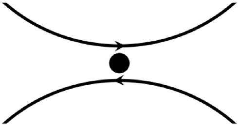
Figure 2.3: The oppositely directed center fluxes in the core of the intersection of a selfintersecting center-vortex loop generate an eddy where an isolated magnetic $Z_{2}$ monopole is located.

Each intersection point carries one unit of magnetic charge, see Fig. 2.3, where each sign is equally likely. The spectrum of excitations is equidistant since the mass of a soliton with $N$ self-interactions is given by $N\Lambda_{C}$, $\Lambda_{C}$ being the Yang-Mills scale. Modulo the charge multiplicities the number of distinct topologies of $N$-fold selfintersecting solitons is given by the number of distinct topologies of connected bubble diagrams with $N$ vertices in a scalar $\lambda\phi^{4}$ quantum field theory. In Fig. 1.1 the topologies of CVLs with up to $N=3$ selfintersections are shown. If subjected to mixing with theories possessing propagating photons the only stable excitations are non-selfintersecting and one-fold selfintersecting CVLs. This is due to the repulsive or attractive forces between the charges of CVLs with more than one selfintersection. CVLs without selfintersection, however, are unstable in the presence of a noisy environment, see Sec. 2.6.

In [10] the potential $V_{C}$ for the macroscopic field $\Phi$ is found to be

$$V_{C}=\overline{\left(\frac{\Lambda_{C}^{3}}{\Phi}-\Lambda_{C}\Phi\right)}\left(\frac{\Lambda_{C}^{3}}{\Phi}-\Lambda_{C}\Phi\right),$$ (2.31)

satisfying the following properties (see also [24]):

(i) $V_{C}$ is invariant under center jumps $\Phi\rightarrow\exp(\mathrm{i}\pi)\Phi$ only;

(ii) it allows for the creation of spin-1/2 fermions by a forward- and backward tunneling which corresponds to local center jumps of $\Phi$’s phase;

(iii) the degenerated minima of $V_{C}$ have zero energy density and are related by local center jumps;

(iv) a mass scale $\Lambda_{C}$ occurs to parameterize the potential $V_{C}$;

(v) $V_{C}$ needs to be real.

The process of relaxation of $\Phi$ to one of the minima of $V_{C}$ is described by the action

$$S=\int\mathrm{d}x^{4}\;\left(\frac{1}{2}\overline{\partial_{\mu}\Phi}\,\partial_{\mu}\Phi-\frac{1}{2}V_{C}\right).$$ (2.32)

Once $\Phi$ has reached $V_{C}$’s minima, quantum fluctuation $\delta\Phi$ are absent because every potential fluctuation would be harder than the maximal resolution.

Neglecting contact interactions between and internal degrees of freedom within solitons as well as long-range interactions between charges mediated by photons, the naive series for the total pressure $P_{C}$ at temperature $T$ represents an asymptotic expansion in powers of a suitably defined coupling coupling constant $\lambda\equiv\exp(-\Lambda_{C}/T)$. That is, the sum

$$P_{C}=\sum_{N=0}^{\infty}P_{C,N}$$ (2.33)

over partial pressures $P_{C,N}$ of spin-1/2 states arising from solitons with $N$ selfintersections seems to converge up to a critical, temperature-dependent value $N_{c}(T)$, but converges when including higher contributions. This signals that the assumption that solitons with arbitrary $N$ are stable breaks down to hold for $N>N_{c}$ as a consequence of contact interactions which increase due to the higher density of intersection points and vortex lines. Though formally divergent, the sum over partial pressures $P_{C,N}$ turns out to be Borel summable for negative (unphysical) values of $\lambda$. The inverse Borel transformation is meromorphic in the entire $\lambda$-plane except for a branch cut along the positive-real axis. Continuation to the physical region $\lambda>0$ leads to a sign-indefinite imaginary part which is smaller than the real part for sufficiently small temperatures. Complex admixtures to the pressure become manifest as turbulence-like phenomena in the plasma and thus violate thermal equilibrium. At zero temperature, the pressure of the ground state is precisely nil. Because of the over-exponential rise of spin-1/2 fermion states with increasing temperature, the imaginary part starts to dominate the pressure and the thermodynamical description of the system begins to fail (violation of spatial homogeneity). That is, at temperature $T_{H}\sim\Lambda_{C}$, the entropy wins over the Boltzmann suppression in energy and the partition function diverges. This is an indication for the Hagedorn transition to the preconfining phase. For details see [25]. Similar behavior is observed for the expansion of the energy density [26]

$$\rho_{C}=\sum_{N=0}^{\infty}\rho_{C,N},$$ (2.34)

where $\rho_{C,N}$ is the energy density of soliton states with $N$ selfintersections and mass $N\Lambda_{C}$.

Demanding for continuity of the negative pressure across the magnetic-center phase transitions yields a relation between $\Lambda_{M}$ and $\Lambda_{C}$:

$$\Lambda_{M}\propto 2^{1/3}\Lambda_{C}.$$ (2.35)

The question may arise whether there are stable selfintersecting vortex-loops in the magnetic phase. By the decay of the macroscopic ground state in the magnetic phase its energy density is used to create selfintersecting CVLs. An $N$-fold twisted CVL possesses a mass $N\Lambda_{C}$, where the Yang-Mills scale is about $\Lambda_{C}\propto T_{H}$. For this reason, the potential in the magnetic phase cannot provide enough energy density to create a selfintersection in the magnetic phase.

2.5 The postulate $\mathrm{SU(2)}_{\mbox{\tiny CMB}}=\mathrm{U(1)}_{Y}$

We have mentioned in Sec. 2.2 that the spatial coarse-graining over the topologically nontrivial sector leads to the emergence of a macroscopic adjoint Higgs field which breaks the fundamental gauge group SU(2) down dynamically to the subgroup U(1). Thereby, two out of three gauge bosons become massive. At $T_{c,E}=13.87\frac{\Lambda_{C}}{2\pi}$, where the electric-magnetic phase transition takes place, the mass of these two gauge field diverges and the massless mode remains exactly massless because radiative corrections are absent due to the decoupling from its heavy partners.

Now consider the U(1)_Y factor of the electroweak gauge group $\mathrm{SU(2)}_{W}\times\mathrm{U(1)}_{Y}$ of the present Standard Model of Particle Physics (SM). In Quantum Electrodynamics (QED), the photon is observed to be unscreened and practically massless ($m_{\gamma}<10^{-14}$ eV) [27]. It is described by the gauge group U(1) the progenitor of which is the U(1)_Y factor. As stated above, there is only a single point in the phase diagram of SU(2) Yang-Mills thermodynamics that exhibits a precisely massless gauge mode: the deconfining-preconfining phase transition at $T_{c,E}$. Therefore, in [10, 23, 28, 29], the postulate was pushed forward that the U(1)_Y factor of the electroweak gauge group is the unbroken subgroup of an SU(2) Yang-Mills theory with a scale comparable to the temperature of the cosmic microwave background (CMB) $T_{\mbox{\tiny{CMB}}}=2.728$ eV. This group is denoted $\mathrm{SU(2)}_{\mbox{\tiny CMB}}$. The photon $\gamma$ in the SM has to be identified with the massless gauge mode of $\mathrm{SU(2)}_{\mbox{\tiny CMB}}$. In analogy to the $W^{\pm}$ gauge bosons of the SM, the remaining two infinitely massive and thus undetectable gauge modes of $\mathrm{SU(2)}_{\mbox{\tiny CMB}}$ are denoted $V^{\pm}$ ($m_{V^{\pm}}=2e\phi$ with $e=\infty$ at $T_{c,E}$). Furthermore, the average temperature of the universe $T_{\mbox{\tiny CMB}}$ is identified with the critical temperature $T_{c,E}$ of $\mathrm{SU(2)}_{\mbox{\tiny CMB}}$. This fixes the only free parameter of the theory, the Yang-Mills scale $\Lambda_{E}$, to $\Lambda_{E}=\frac{2\pi}{13.87}T_{\mbox{\tiny CMB}}=1.065\times 10^{-4}$ eV. For temperatures much above $T_{c,E}$, the effects of $V^{\pm}$ are completely negligible, whereas for temperatures a few times of $T_{\mbox{\tiny CMB}}$, these lead to a visible modification of the black-body spectrum at low frequencies (spectral gap) [29, 30]. The spectral gap could also provide for an explanation why old (estimated age $\sim$ 50 million years), cold (mean brightness temperature $\sim 20$ K) and dilute (number density $\sim 1.5$ cm³) clouds in between the spiral arms of the outer galaxy are composed of atomic instead of molecular hydrogen, and why these clouds are stable [31].

Regarding the transition towards the preconfining phase, the postulate $\mathrm{SU(2)}_{\mbox{\tiny CMB}}=\mathrm{U(1)}_{Y}$ implies that the photon will acquire a Meißner mass because of the coupling to the newly emerging superconducting ground state (condensate of magnetic monopoles). The system, however, remains in a supercooled state down to $T=12.15\frac{\Lambda_{E}}{2\pi}$ due to the shift in energy density at $T_{c,E}$ (additional degree of freedom), see also Fig. 2.2. In [23] an upper bound for the time the photon remains massless was estimated to be $\sim 2.2$ billion years. The observed intergalactic magnetic fields can possibly be explained by the electric-magnetic phase transition. Conventional superconductors consist of a Cooper-pair condensate of electric charges and expel magnetic fields from their interior (Meißner effect). If the occurrence of intergalactic magnetic fields is addressed to the emergence of a superconducting ground state, this leads to the conclusion that a magnetically charged object in the gauge group $\mathrm{SU(2)}_{\mbox{\tiny CMB}}$ is interpreted as an electrically charged object with respect to U(1)_Y. Therefore, the ground state of the magnetic phase is a condensate of electrically charged monopoles and antimonopoles with respect to U(1)_Y, and thus generates intergalactic magnetic fields.

2.6 Motion by curvature

Here, we would like to illustrate how the curve shrinking process is induced by the curvature of a CVL. Recall that the vortex loop is generated by the bending of a straight ANO vortex line which exhibits isotropic pressure perpendicular to its symmetry axis.

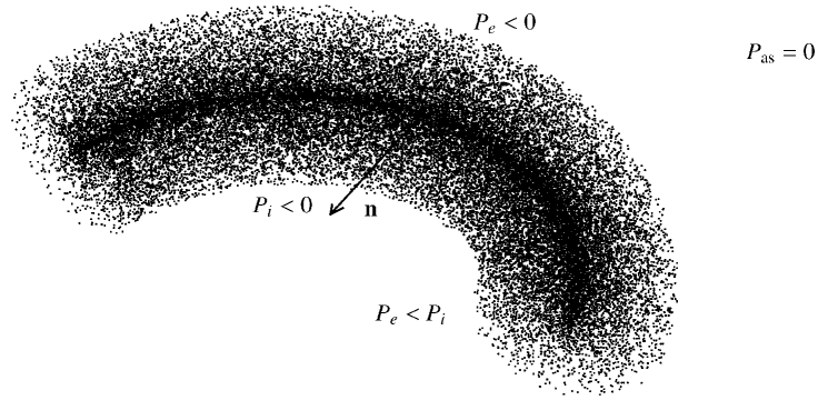
Figure 2.4: Highly space-resolved snapshot of a segment of a center-vortex loop. The pressure $P_{i}$ in the region pointed to by the normal vector $\mathbf{n}$ is more negative than the pressure $P_{e}$ thus leading to a motion of the segment along $\mathbf{n}$.

Now consider a situation where a CVL of an isolated SU(2) Yang-Mills theory is (locally) embedded into a flat two-dimensional surface at $m_{\scriptscriptstyle D}<\infty$ and $d>0$. Then, a hypothetical observer measuring a positive (negative) curvature of a segment of the vortex line experiences more (less) negative pressure in the intermediate vicinity of this curve segment (see Sec. 2.4) leading to its motion towards (away from) the observer, see Fig. 2.4. The (inward directed) velocity of a point in the vortex core will be a monotonic function of the curvature at this point. On average, this shrinks the CVL. Alternatively, one may globally consider the limit $m_{\scriptscriptstyle D}\to\infty$, $d\to 0$, that is the confining phase, but now taking into account the effects of an environment that locally relaxes this limit (by collisions) and thus also induces curve shrinking. This situation is described by a curve shrinking flow in the dimensionless parameter $\tau$

$$\partial_{\tau}\vec{x}(\xi,\tau)=\frac{1}{\sigma}\,\partial^{2}_{\xi}\vec{x}(\xi,\tau),$$ (2.36)

where $\vec{x}$ is a point on the planar CVL, $\xi$ is arc length, and $\sigma$ a string tension effectively expressing the distortions induced by the (noisy) environment. After a rescaling to dimensionless variables,

$$\mathbf{x}\equiv\sqrt{\sigma}\vec{x}\qquad\textnormal{and}\qquad s=\sqrt{\sigma}\xi,$$ (2.37)

flow equation (2.36) assumes the form:

$$\partial_{\tau}\mathbf{x}(s,\tau)=\partial_{s}^{2}\mathbf{x}(s,\tau).$$ (2.38)

In the following sections, we will resort to the dimensionless flow equation.

Chapter 3 Mathematical Prerequisites: Curve shrinking flow

In the 1970s, William Thurston developed a program for the classification of three-dimensional manifolds. It had a great impact in the field of three-dimensional topology and revealed a very strong connection between low-dimensional topology and differential geometry, especially between hyperbolic geometry and Kleinian groups [32, 33].

Now consider a smooth closed (that is, compact and without boundary) manifold $\mathcal{M}$ equipped with a smooth time-dependent Riemannian metric $g(\tau)$. A (topological) manifold is a topological space which is locally homeomorphic to a Euclidean space, but with an generally more complicated global structure. A manifold equipped with a Riemannian metric $g$ is a real differentiable manifold $\mathcal{M}$, in which each tangent space is endowed with an inner product $g$ in a manner that varies smoothly from point to point. It should be noted that not every manifold admits a geometry. The Ricci flow is a means of processing the metric $g$ by the evolution of $g$ under the following partial differential equation (PDE)

$$\frac{\partial}{\partial\tau}g(\tau)=-2\mathrm{Ric}(g),$$ (3.1)

where Ric is the Ricci curvature. In local coordinates the coefficients $R_{ij}$ of the Ricci curvature tensor are given by a contraction of the Riemannian curvature tensor $R^{i}{}_{jkl}$, $R_{ij}=R^{k}{}_{ikj}$. Roughly speaking, the Ricci-flow contracts regions of positive curvature and expands those of negative curvature, thereby smoothing out irregularities in the metric. In this spirit, it is formally analogous to the diffusion of heat that describes how an irregular temperature distribution in a given region tends to become more homogeneous over time. An example of its application is the proof of the two-dimensional uniformization theorem, which states that any surface admits a Riemannian metric of constant Gaussian curvature. Here, the (suitably renormalized) Ricci flow is used to conformally deform a two-dimensional metric on $\mathcal{M}$ into one of constant curvature [34]. Richard Hamilton introduced the Ricci flow with the intention to gain insight into the geometrization conjecture proposed by William Thurston in 1980 [35]. The geometrization conjecture is the analogue for three-manifolds of the uniformization theorem for surfaces and implies several other conjectures, such as Thurston’s elliptization conjecture or the Poincaré conjecture. Let us first consider the Poincaré conjecture, which was originally posed as a question at the end of an article by Henri Poincaré in 1904. In its standard form, it states that every simply connected, compact three-manifold without boundary is homeomorphic to the three-sphere. A more precise phrasing is that the fundamental group of a closed three-manifold $\mathcal{M}$ is trivial, if and only if $\mathcal{M}$ is homeomorphic to the three-sphere. Now, the geometrization conjecture concerns the topological classification of three-dimensional smooth manifolds. The original phrasing of Thurston goes as follows [35]: “The interior of every compact 3-manifold has a canonical decomposition into pieces which have geometric structures”. In three dimension there are precisely eight geometric structures called the eight Thurston (model) geometries (involving the spherical geometry $S^{3}$, the Euclidean geometry $\mathbb{R}^{3}$, the hyperbolic geometry $\mathbb{H}^{3}$, the geometry of $S^{2}\times\mathbb{R}$, the geometry of $\mathbb{H}^{2}\times\mathbb{R}$, the geometry of the universal cover of $SL_{2}(\mathbb{R})$, the nil geometry and finally the sol geometry). The canonical decomposition is carried out in two steps. In the first stage, also referred to as the prime decomposition, one cuts a three-manifold $\mathcal{M}$ along two-spheres embedded in $\mathcal{M}$ such that neither of the obtained manifolds is a three-ball, then one glues three-balls to the resulting boundary components. This decomposition is unique up to the sequence and additional three-balls. The second stage involves cutting along certain tori that are nontrivially embedded in $\mathcal{M}$ obtaining a three-manifold the boundary of which consists of tori. Hamilton’s basic idea was to place an arbitrary metric $g$ on a given smooth manifold $\mathcal{M}$ and to dynamically deform $\mathcal{M}$ by the Ricci flow to yield one of Thurston’s geometric structures. Hamilton succeeded in proving that a closed three-dimensional manifold, which carries a metric of positive Ricci curvature, is a spherical space form that acts like an attractor under the Ricci flow [36]. This is known as the Hamilton theorem. However, in general, the Ricci flow can be expected to develop a singularity in finite time. Then, in a series of eprints starting in 2002, Grigori Perelman sketched a proof for the geometrization conjecture [37]. Thereby, Perelman modified Hamilton’s program to prove Thurston’s geometrization conjecture by stopping the Ricci flow once a singularity has been formed, then carefully performing ‘surgery’ on the evolved manifold, systematically excising singular regions before continuing the flow. This is called Ricci flow with surgery.

The results obtained in this thesis heavily depend on the important work on the curve shortening flow done by Gage and Hamilton [38], and Grayson [39, 40]. The curve shortening flow, also known as heat equation on immersions, is the one-dimensional analogue to the Ricci flow and originally inspired Hamilton in the development of the Ricci flow. Let us now consider the properties of curve shrinking flows in two and three space dimensions.

3.1 Embedded curves without selfintersection

3.1.1 Planar curves

Consider a family of smooth, closed curves $\mathbf{x}(s,\tau)$ of length $L$ embedded in a two-dimensional flat plane $\mathbb{R}^{2}$, where $\mathbf{x}$ is a point along the curve, $s\in[0,L]$ is the arc length that is unique only up to a constant and $\tau\in[0,T]$ the flow parameter which parametrizes the family. The initial curve $\mathbf{x}(s,0)$ evolves as a function of ‘time’ $\tau$ to $\mathbf{x}(s,\tau)$. The Euclidean curve shortening flow is defined as

$$\partial_{\tau}\mathbf{x}(s,\tau)=\partial_{s}^{2}\mathbf{x}(s,\tau)\equiv k(s,\tau)\,\mathbf{n}(s,\tau),$$ (3.2)

where the derivative $\partial_{\tau}:=\frac{\partial}{\partial\tau}$ is taken along a fixed value of $s$. This is a parabolic, nonlinear second-order partial differential equation, where $\mathbf{n}$ is the inward-pointing Euclidean unit normal and $k$ the scalar curvature, defined as

$$k(s,\tau)=|\partial_{s}^{2}\mathbf{x}(s,\tau)|=\det(\partial_{s}\mathbf{x}(s,\tau),\partial_{s}^{2}\mathbf{x}(s,\tau)),$$ (3.3)

with $|\mathbf{v}|\equiv\sqrt{\mathbf{v}\cdot\mathbf{v}}$, $\mathbf{v}\cdot\mathbf{w}$ denoting the Euclidean scalar product, and $\det(\cdot,\cdot)$ denotes the determinant of the $2\times 2$ matrix created by two $2\times 1$ vectors. It is a standard result for parabolic equations that solutions exist for a short time and are unique. In the curve shortening flow, the curve $\mathbf{x}(s,\tau)$ is deformed along its unit normal $\mathbf{n}(s,\tau)$ at a rate that is proportional to its curvature $k(s,\tau)$. This flow deserves the attribute curve shortening, because its flow lines in the space of closed curves are tangent to the gradient for the curve length functional, see Eq. (3.17). For the remainder of this section, we assume that a solution to Eq. (3.2) exists on the maximal time interval $[0,T)$. A more visual description of this flow is the evolution of an elastic band in a viscous medium. If the tension in the elastic is kept constant then its behavior is approximately determined by Eq. (3.2), see also Fig. 3.1.

Figure 3.1: The Euclidean curve shortening flow. The arrows point towards the unit normal $\mathbf{n}$ and the length of the arrows is proportional to the curvature $k$.

Since motion normal to the curve affects arc length, $s$ is not preserved under curve shrinking. Thus, $s$ and $\tau$ are not independent and commute according to the following rule

$$\partial_{\tau}\partial_{s}=\partial_{s}\partial_{\tau}+k^{2}\partial_{s}.$$ (3.4)

Therefore, we introduce the curve parameter $u$ (modulo $2\pi$) related to $s$ by

$$\mathrm{d}s=\left|\partial_{u}\mathbf{x}\right|\mathrm{d}u.$$ (3.5)

The quantity $|\partial_{u}\mathbf{x}|$ can also be thought of as an arc length density. Actually, Eq. (3.5) defines $s$. The operator $\partial_{s}$ then writes as

$$\partial_{s}=\frac{1}{\left|\partial_{u}\mathbf{x}\right|}\partial_{u}.$$ (3.6)

In the following, we resort to a slight abuse of notation by using the same symbol $\mathbf{x}$ for the functional dependence on $u$ or $s$. Let us now introduce coordinates in $\mathbb{R}^{2}$, $\mathbf{x}(u,\tau)=(x(u,\tau),y(u,\tau))^{T}$ (where $T$ denotes the transpose). The tangent vector to the curve is given by $\partial_{u}\mathbf{x}$, and thus we define the unit tangent $t$ vector as

$$\mathbf{t}(u,\tau):=\frac{\partial_{u}\mathbf{x}}{|\partial_{u}\mathbf{x}|}=\frac{1}{|\partial_{u}\mathbf{x}|}\left(\begin{array}[]{c}\partial_{u}x\\ \partial_{u}y\end{array}\right).$$ (3.7)

The unit normal is then given by

$$\mathbf{n}(u,\tau):=\frac{1}{|\partial_{u}\mathbf{x}|}\left(\begin{array}[]{c}-\partial_{u}y\\ \partial_{u}x\end{array}\right).$$ (3.8)

The unit tangent and normal vectors are written in terms of arc length $s$ as

$$\mathbf{t}(s,\tau)=\left(\begin{array}[]{c}\partial_{s}x\\ \partial_{s}y\end{array}\right),\qquad\textnormal{and}\qquad\mathbf{n}(s,\tau)=\left(\begin{array}[]{c}-\partial_{s}y\\ \partial_{s}x\end{array}\right).$$ (3.9)

So we can write the Frenet-Serret formulas, which describe the kinematic properties of a point (particle) that moves along the planar curve $\mathbf{x}$ as

$$\frac{\partial}{\partial s}\left(\begin{array}[]{c}\mathbf{t}\\ \mathbf{n}\end{array}\right)=\left(\begin{array}[]{cc}0&k\\ -k&0\end{array}\right)\left(\begin{array}[]{c}\mathbf{t}\\ \mathbf{n}\end{array}\right),$$ (3.10)

where the curvature, when expressed in coordinates, is

$$k(s,\tau)=\partial_{s}x\,\partial_{s}^{2}y-\partial_{s}^{2}x\,\partial_{s}y.$$ (3.11)

The circumference of the curve $L$ at time $\tau$ is defined as

$$L(\tau)\equiv\int_{0}^{L(\tau)}\mathrm{d}s=\int_{0}^{2\pi}\mathrm{d}u\,\left|\partial_{u}\mathbf{x}(u,\tau)\right|.$$ (3.12)

The evolution of $L$ under the flow is given by

$$\dot{L}(\tau):=\frac{\mathrm{d}L(\tau)}{\mathrm{d}\tau}\equiv-\int_{0}^{L(\tau)}\mathrm{d}s\,k^{2}=-\int_{0}^{2\pi}\mathrm{d}u\left|\partial_{u}\mathbf{x}\right|k^{2}.$$ (3.13)

For the area $A$ enclosed by the curve we have

$$A(\tau)\equiv\frac{1}{2}\left|\int_{0}^{L(\tau)}\mathrm{d}s\;\mathbf{x}(s,\tau)\cdot\mathbf{n}(s,\tau)\right|.$$ (3.14)

Surprisingly, the time derivative of the enclosed area remains constant under curve shrinking,

$$\dot{A}(\tau):=\frac{\mathrm{d}A(\tau)}{\mathrm{d}\tau}=-2\pi.$$ (3.15)

For planar curves, the decreasing integral $\int_{0}^{L}\mathrm{d}s\,|k|$ measures the total change in angle. In the special case of convex planar curves, $\int_{0}^{L}\mathrm{d}s\,|k|=\int_{0}^{L}\mathrm{d}s\,k$ measures the winding number of the curve and is an invariant of the flow (until a singularity develops).

In [41], Grayson stated that under the flow Eq. (3.2) ‘the curve is shrinking as fast as it can using only local information’. Let us see how this statement can be understood. Consider the curve length $L(\tau)=\int_{0}^{2\pi}\mathrm{d}u\,|\partial_{u}\mathbf{x}|$. To take the time derivative of $L$ we differentiate $|\partial_{u}\mathbf{x}|^{2}$ with respect to $\tau$ and obtain

$$\partial_{\tau}|\partial_{u}\mathbf{x}|=\frac{1}{|\partial_{u}\mathbf{x}|}\partial_{u}\mathbf{x}\cdot\partial_{\tau}\partial_{u}\mathbf{x}.$$ (3.16)

Substituting this into $\dot{L}(\tau)$ and integrating by parts, we obtain the following expression for the rate of decrease of curve length

$$\dot{L}(\tau)=-\int_{0}^{L(\tau)}\mathrm{d}s\,k\,\mathbf{n}\cdot\partial_{\tau}\mathbf{x}.$$ (3.17)

Therefore, Eq. (3.2) expresses the local condition that the rate of decrease of $L(\tau)$ is maximal with respect to a variation of the direction of the velocity $\partial_{\tau}\mathbf{x}$ of a given point on the curve at fixed magnitude $|\partial_{\tau}\mathbf{x}|$ [42]. However, the magnitude $|\partial_{\tau}\mathbf{x}|$ is not in general the speed which maximizes $\dot{L}(t)$.

Setting $A(\tau=0)\equiv A_{0}$, the solution to Eq. (3.15) is

$$A(\tau)=A_{0}-2\pi\,\tau.$$ (3.18)

By virtue of Eq. (3.18) the critical value $T$, where $A$ and with it the curve vanishes, is related to $A_{0}$ as

$$T=\frac{A_{0}}{2\pi}.$$ (3.19)

The isoperimetric ratio is defined as $\frac{L^{2}}{A}$, and the isoperimetric inequality states that

$$\frac{L(\tau)^{2}}{A(\tau)}\geq 4\pi.$$ (3.20)

Equality is achieved if and only if the curve is a circle. Therefore, one can consider it a measure of ‘how circular’ the curve is.

In 1983, Gage showed that when a smooth convex curve evolves according to Eq. (3.2), the isoperimetric ratio $\frac{L^{2}}{A}$ decreases, so that if $A\rightarrow 0$, then $L\rightarrow 0$ and the curve shrinks to a point [43]. In 1984, Gage showed that a convex curve is becoming circular and $\frac{L^{2}}{A}$ approaches $4\pi$, as the enclosed area approaches zero, provided that the curvature does not blow up prematurely, that is the curve does not form a cusp [44]. As a consequence, the ratio $\frac{R_{\mathrm{out}}}{R_{\mathrm{in}}}$ of the circumscribed ratio to the inscribed ratio converges to unity. This can be considered a $C^{0}$-convergence to the circle. Hence, in the absence of singularities, a strictly convex and embedded curve remains convex and embedded under the evolution.

In 1986, Gage and Hamilton showed that for convex curves the curvature does not blow up prematurely for $\lim_{\tau\rightarrow T}A(\tau)=0$ [38]. Thus, the curve remains convex and becomes circular, as it shrinks to a point for $\tau\nearrow T$, where $0<T<\infty$. The curve shrinks to a circle in the sense that:

(i) the ratio $\frac{R_{\mathrm{out}}}{R_{\mathrm{in}}}$ approaches unity;

(ii) the ratio of the maximum curvature to the minimum curvature $\frac{k_{\mathrm{max}}}{k_{\mathrm{min}}}$ approaches unity ($C^{2}$-convergence);

(iii) the higher order derivatives of the curvature $k$ converge to zero uniformly ($C^{\infty}$-convergence).

In 1987, Grayson showed that embedded (non-selfintersecting) planar curves become convex before $T$ without developing singularities [41]. Thus, this completes the proof of the well known Gage-Hamilton-Grayson theorem that curve shortening determined by Eq. (3.2) shrinks embedded plane curves smoothly to points, with round limiting shape. It is important to note that some planar curves, which are immersed but not embedded will surely develop singularities, e.g. the figure-eight of Sec. 3.2 or the Limaçon of Pascal.

Consider the set of all Euclidean transformations in $\mathbb{R}^{2}$, that is the set of all rotations, translations and reflections of a figure in $\mathbb{R}^{2}$. Such a transformation $ET:\mathbb{R}^{2}\rightarrow\mathbb{R}^{2}$ is a function of the form

$$ET(\mathbf{x})=U\mathbf{x}+a,$$ (3.21)

where $U$ is an orthogonal $2\times 2$ matrix and $a\in\mathbb{R}^{2}$. The Euclidean curve shortening flow is defined in terms of the Euclidean curvature $k$ and the Euclidean unit normal $\mathbf{n}$ that are invariant under Euclidean transformations $ET$.

3.1.2 Space curves

There are several possibilities of generalizing the curve shortening flow. One is the mean curvature flow, which is the generalization of Eq. (3.2) for hypersurfaces. In this case, the results of Sec. 3.1.1 continue to hold for convex curves, but for non-convex curves they do not [45].

For our purposes, it is more interesting to look at the extension of the curve shortening flow for curves embedded in the three-dimensional Euclidean space $\mathbb{R}^{3}$. Consider a continuous, differentiable (and not necessarily closed) space curve $\mathbf{x}(s,\tau)$ embedded in $\mathbb{R}^{3}$. The tangent, normal and binormal unit vectors are denoted $\mathbf{t}$, $\mathbf{n}$ and $\mathbf{b}$, respectively, also called Frenet-Serret frame, and defined as follows:

$\mathbf{t}$ is the unit vector tangent to the curve, pointing in the direction of motion: $\mathbf{t}=\partial_{s}\mathbf{x}$;

$\mathbf{n}$ is the normalized derivative of $\mathbf{t}$ with respect to the arc length $s$ of the curve: $\mathbf{n}=\frac{\partial_{s}\mathbf{t}}{|\partial_{s}\mathbf{t}|}$;

$\mathbf{b}$ is the cross product of $\mathbf{t}$ and $\mathbf{n}$: $\mathbf{b}=\mathbf{t}\times\mathbf{n}$.

The Frenet-Serret formulas for a point on the space curve are given by

$$\frac{\partial}{\partial s}\left(\begin{array}[]{c}\mathbf{t}\\ \mathbf{n}\\ \mathbf{b}\end{array}\right)=\left(\begin{array}[]{ccc}0&k&0\\ -k&0&t\\ 0&-t&0\end{array}\right)\cdot\left(\begin{array}[]{c}\mathbf{t}\\ \mathbf{n}\\ \mathbf{b}\end{array}\right),$$ (3.22)

where $k$ is the curvature and $t$ the torsion. The Frenet-Serret formulas effectively define the curvature and torsion of a space curve. It should be noted that the existence of a Frenet-Serret frame requires $|k\mathbf{n}|^{2}>0$. That is, a particle traveling along the curve must experience acceleration. The evolution equation for space curve assumes the same form as Eq. (3.2),

$$\partial_{\tau}\mathbf{x}(s,\tau)=k(s,\tau)\mathbf{n}(s,\tau).$$ (3.23)

The unit normal $\mathbf{n}$ is not always defined, though $k\mathbf{n}$ always makes sense. It was shown by Altschuler and Grayson that solutions to the space curve flow exist until the curvature becomes unbounded. However, space curves may not remain embedded in general, and singularities will develop in the case of closed curves. A phenomenon of space curve evolution is that inflection points ($k=0$) may develop during a time interval on which the curvature is bounded. When this happens the curvature becomes zero and the torsion infinite at a point. Nevertheless the curve remains embedded since the flow ignores these types of singularities in the torsion [46, 47]. A rather surprising property of space curve evolution is, that the formation of a singularity is a planar phenomenon. A space curve is said to be planar at a point $(s^{\prime},\tau^{\prime})$ if the ratio of torsion and curvature vanishes, $\frac{t}{k}(s^{\prime},\tau^{\prime})=0$. In [46], Altschuler showed that if a space curve develops a singularity at $(s^{\prime},\tau^{\prime})$, then $\lim_{(s,\tau)\rightarrow(s^{\prime},\tau^{\prime})}\frac{t}{k}(s,\tau)=0$. Furthermore, Altschuler showed that the space curve is either asymptotic ($\tau\rightarrow\infty$) to a planar solution which moves by homothety (self-similarity), or a rescaling of the solution along the singularity converges in $C^{\infty}$ to a limiting solution $\mathbf{x}(s,\tau=\infty)$ [46], where $\mathbf{x}(s,\tau=\infty)$ is the family of planar, convex curves. The most trivial case of a curve moving by homothety is the circle shrinking down to a point. It should be noted that the conjecture due to Grayson, that singularity formation is a planar phenomenon, can be proven without using the language of rescalings.

3.2 Immersed curves with one selfintersection

When a closed curve immersed in a plane evolves by its curvature according to Eq. (3.2), it remains smooth until its curvature blows up. From Sec. 3.1.1, we know that an embedded closed curve cannot develop a singularity until it shrinks to a point, where the limiting shape of the curve converges in $C^{\infty}$ to circle. In marked contrast to this behavior, it was shown by Grayson that an immersed curve can evolve by the curvature flow such that its area vanishes, but its isoperimetric ratio converges to $\infty$. Such a curve, namely a figure-eight, was investigated in [40]. A figure-eight is the simplest non-embedded curve and is defined to be a smooth immersion into the plane with exactly one double point, and a total rotation number zero,

$$\int_{0}^{L}\mathrm{d}s\,k=0.$$ (3.24)

Here, $s$ is arc length, $L$ the curve length and $k$ the scalar curvature. Such a curve divides the plane into three disjoint areas two of which are finite and denoted (the unsigned areas) $A_{1}$ and $A_{2}$. Let $\mathbf{x}(s,\tau=0)$ be figure-eight which evolves to $\mathbf{x}(s,\tau)$ according Eq. (3.2) for $0\leq\tau<T$. The curvature is unbounded as $\tau\rightarrow T$. The main result of [40] is that the isoperimetric ratio $\frac{L^{2}}{A}$ converges to $\infty$ as $\tau\rightarrow T$ if and only if the loops bound regions of equal area, $A_{1}(0)=A_{2}(0)$. This in turn implies that $\frac{L^{2}}{A}$ for a curve with unequal-area loops is bounded as $\tau\rightarrow T$.

Since for immersed curves the number of double points is a non-increasing function of time [48], a figure-eight remains a figure-eight until one of its loops collapses or the flow encounters a singularity. The curve stays smooth and the flow continues until $A_{1}$ or $A_{2}$ converge to zero. For the total area $A$ of a figure-eight we have

$$A(\tau)=A_{1}(\tau)+A_{2}(\tau).$$ (3.25)

The time derivative of the area enclosed by one of loop of the curve is equal to $-|\int\mathrm{d}s\,k|$ over the loop. Unlike the case of a non-selfintersecting curve, the rate of change of the total area is not longer constant, but constrained as

$$-4\pi\leq\frac{\mathrm{d}A(\tau)}{\mathrm{d}\tau}\leq-2\pi.$$ (3.26)

However, we have the nice property of figure-eights that the difference of areas bounded by the two loops of $\mathbf{x}(s,\tau)$ remains constant under the flow evolution:

$$A_{1}(\tau)-A_{2}(\tau)=\mathrm{const}.$$ (3.27)

Aside from a number of applications in differential geometry, curve shortening flows are also used in multi-agent systems, such as mobile autonomous robots [42], in image processing where the flow provides an efficient way to smooth curves representing the contours of objects, or in computer vision. For a complete account of many of the results of curve shrinking see [45, 49].

In the following, we suppress the functional dependence on $u$ in the argument of $\mathbf{x}$ and $\mathbf{n}$ and write $\mathbf{x}(\tau):=\mathbf{x}(u,\tau)$ and $\mathbf{u}(u,\tau):=\mathbf{n}(\tau)$

Chapter 4 Non-selfintersecting center-vortex loops

We apply curve shrinking to the $N=0$ sector in the sense of Sec. 2.6. It should be noticed that the restriction of the motion of a CVL to a two-dimensional flat plane is a major assumption which needs to be supplemented by additional physical arguments for its validity.

4.1 Wilsonian renormalization-group flow

In this section, we exploit the concept of renormalization-group transformations to yield an effective ‘action’ that enables us to compute statistical quantities. The renormalization group allows one to investigate the change in the physical parameters of a system which is associated with the change in scale (energy or resolution) and necessary to keep the physics constant. In our case, the change of scale corresponds to a change of the resolution $Q$ used to probe the system. Here, the resolution $Q$ is a strictly monotonic decreasing function of the flow parameter $\tau$. The change in parameters of the effective ‘action’ is implicitly determined by a renormalization-group flow in $\tau$.

4.1.1 Geometric partition function

Let us now interpret the process of curve shrinking determined by Eq. (3.2) as a renormalization-group transformation of a statistical ensemble made up of planar $N=0$ CVLs. A partition function, which is the sum over suitable defined weights of the members in the ensemble, is considered to be invariant under a decrease of resolution $Q$ determined by the flow parameter $\tau$. Physically, $\tau$ is a monotonically decreasing function of $Q/Q_{0}$, where $Q$ ($Q_{0})$ are mass scales associated with the actual (initial) resolution applied to the system. The role of $Q$ can also be played by the finite temperature of a reservoir that is coupled to the system.

To define a suitable weight, we devise an ansatz for the effective ‘action’ $S=S[\mathbf{x}(\tau)]$ in geometric terms of the curves in the ensemble, since these are the only accessible quantities in the system of isolated non-interacting CVLs. The ‘action’ as a functional of $\mathbf{x}$ is expressible in terms of integrals over local densities in $s$. Furthermore, we take advantage of the following symmetries the action should possess:

(i) scaling symmetry $\mathbf{x}\to\lambda\mathbf{x},\ \lambda\in\mathbb{R}_{+}$: for both conformal limits, $\lambda\to\infty$ and $\lambda\to 0$, where the curves at fixed $L$ gets unobservable since $\lambda L\to\infty$ and $\lambda L\to 0$, the ‘action’ $S$ should be invariant under further finite rescalings (decoupling of the fixed length scale $\sigma^{-1/2}$);

(ii) Euclidean point symmetry in $\mathbb{R}^{2}$, that is the group of all rotations, translations and reflections of a figure (curve) in the plane: sufficient but not necessary for this is a representation of $S$ in terms of integrals over scalar densities with respect to these symmetries. That is, the ‘action’ density should be expressible as a expansion in series involving products of Euclidean scalar products of $\frac{\partial^{n}}{\partial s^{n}}\mathbf{x},\ n\in\mathbb{N}^{+},$ or constancy. However, scalar integrals can be constructed which involve non-scalar densities. For instance, consider the area $A$ enclosed by curve and given by

$$A(\tau)=\frac{1}{2}\left|\int_{0}^{L(\tau)}\mathrm{d}s\;\mathbf{x}(\tau)\cdot\mathbf{n}(\tau)\right|.$$ (4.1)

The density $\mathbf{x}\cdot\mathbf{n}$ in this expression is not a scalar under translations.

We now decompose the effective ‘action’ into a conformal and a non-conformal factor

$$S=F_{c}\times F_{nc}\;,$$ (4.2)

where in addition to Euclidean point symmetry $F_{c}$ is invariant under $\mathbf{x}\to\lambda\mathbf{x}$, whereas $F_{nc}$ is not. In principle, infinitely many operators can be defined to contribute to $F_{c}$. Since the evolution generates circles for $\tau\nearrow T$ and thus homogenizes the curvature, higher derivatives of $k$ with respect to $s$ rapidly converge to zero [38]. We expect this to be true also for Euclidean scalar products involving higher derivatives $\frac{\partial^{n}}{\partial s^{n}}\mathbf{x}$. To yield conformally invariant expressions such integrals need to be multiplied by powers of $\sqrt{A}$ and/or $L$ or the inverse of integrals involving lower derivatives. At this stage, we are not able to constrain the expansion in derivatives by additional physical or mathematical arguments. To be pragmatic, we simply set $F_{c}$ equal to the isoperimetric ratio:

$$F_{c}(\tau)\equiv\frac{L(\tau)^{2}}{A(\tau)}\,.$$ (4.3)

We consider the non-conformal factor $F_{nc}$ in $S$ as a formal Taylor expansion in inverse powers of $L$ or $A$ due to the conformal invariance of the curve for $L,A\rightarrow\infty$ and $L,A\rightarrow 0$. Since the renormalization-group evolution of the effective ‘action’ is driven by the curve shortening flow of each member in the ensemble, we allow for an explicit $\tau$ dependence of the coefficient $c$ of the lowest nontrivial power $\frac{1}{L}$. The idea is to include the contribution of higher-order operators, that do not exhibit an explicit $\tau$ dependence, into a resolution dependence of the coefficient of the lower-dimensional operators. Thus, we make the following ansatz

$$F_{nc}(\tau)=1+\frac{c(\tau)}{L(\tau)}\,.$$ (4.4)

The initial value $c(\tau=0)$ is determined from a physical boundary condition such as the mean length $\bar{L}$ at $\tau=0$ which determines the mean mass $\bar{m}$ of a $N=0$ CVL as $\bar{m}=\sigma\bar{L}$. We have also considered a modified factor

$$F_{nc}(\tau)=1+\frac{c(\tau)}{A(\tau)}$$ (4.5)

in the ansatz for the ‘action’ in Eq. (4.2).

For later use, we investigate the behavior of $F_{nc}(\tau)$ for $\tau\nearrow T$ for an ensemble consisting of a single curve only and require the independence of the ‘partition function’ under changes in $\tau$. Using Eq. (3.18) in the vicinity of $\tau=T$, where the limiting of curve is a circle with radius $R$, we have

$$L(\tau)=2\pi R=\sqrt{8}\pi\,\sqrt{T-\tau}\,.$$ (4.6)

Since $F_{c}(\tau\nearrow T)=4\pi$, independence of the ‘partition function’ under the flow in $\tau$ implies that

$$c(\tau)\propto\sqrt{T-\tau}\,.$$ (4.7)

That is, $F_{nc}$ approaches a constant value for $\tau\nearrow T$ which brings us back to the conformal limit by a finite renormalization of the conformal part $F_{c}$ of the effective ‘action’. In this parametrization of $S$, the coefficient $c(\tau)$ can thus be regarded as an order parameter for conformal symmetry with a mean-field critical exponent.

4.1.2 Effective ‘action’

We now want to derive an effective ‘action’ $S[\mathbf{x}(\tau)]$ resulting from a partition function $Z$ for a nontrivial ensemble $E$. The partition function $Z_{M}$ is defined as the average

$$Z_{M}=\sum_{i=1}^{M}\exp\left(-S[\mathbf{x}_{i}(\tau)]\right)$$ (4.8)

over the ensemble $E=\{\mathbf{x}_{1},\dots\,\mathbf{x}_{M}\}$. $E_{M}$ denotes an ensemble consisting of $M$ curves where $E_{M}$ is obtained from $E_{M-1}$ by adding a new curve $\mathbf{x}_{M}(u,\tau)$. We are interested in a situation where all curves in $E_{M}$ shrink to a point at the same value $\tau=T$. Because of $T=A_{0}/(2\pi)$, we demand that at $\tau=0$ all curves in $E_{M}$ have the same initial area $A_{0}$. The effective ‘action’ $S$ in Eq. (4.2) (when associated with the ensemble $E_{M}$ we will denote it as $S_{M}$, and the corresponding coefficient $c_{M}$) is determined by the function $c_{M}(\tau)$, compare with Eq. (4.4), the flow of which follows from the requirement of $\tau$-independence of $Z_{M}$:

$$\frac{d}{d\tau}Z_{M}=0\,.$$ (4.9)

This is an implicit, first-order ordinary differential equation for $c_{M}(\tau)$, which is in need for an initial condition $c_{0,M}=c_{M}(\tau=0)$. An obvious choice of initial condition is to demand that the statistic mean length $\bar{L}(\tau)$, defined as

$$\bar{L}_{M}(\tau)\equiv\frac{1}{Z_{M}(\tau)}\sum_{i=1}^{M}L[\mathbf{x}_{i}(\tau)]\,\exp\left(-S_{M}[\mathbf{x}_{i}(\tau)]\right),$$ (4.10)

coincides with the geometric mean length $\tilde{L}_{M}(\tau)$ defined as

$$\tilde{L}_{M}(\tau)\equiv\frac{1}{M}\sum_{i=1}^{M}L[\mathbf{x}_{i}(\tau)]$$ (4.11)

at $\tau=0$:

$$\bar{L}_{M}(0)=\tilde{L}_{M}(0).$$ (4.12)

From this initial condition a value for $c_{0,M}$ follows. In the case of the modified ‘action’ in Eq. (4.5), the choice of initial condition $\bar{L}_{M}(\tau=0)=\tilde{L}_{M}(\tau=0)$ leads to $F_{nc}(\tau)\equiv 0$ which is equivalent to a uniform distribution. This is because initial condition (4.12) is identically fulfilled for the modified ‘action’ if $c(0)=-A_{0}$ is chosen, then setting $c(\tau)=-A(\tau)$ solves $\mathrm{d}Z_{M}/\mathrm{d}t=0$ trivially. While the geometric effective ‘action’ is thus profoundly different for such a modification of $F_{nc}(\tau)$, physical results such as the evolution of the variance of the position of the ‘center of mass’ agree remarkably well, see Sec. 4.2.4. We conclude, that the geometric effective ‘action’ itself has no physical interpretation in contrast to quantum field theory and conventional statistical mechanics where the action in principle is related to the physical properties of a given member of the ensemble. Rather, going from one ansatz for $S_{M}$ to another describes a particular way of redistributing the weight in the ensemble which seems to have no significant impact on the physics.

4.2 Results of simulation

4.2.1 Preparation of ensemble

For the curves depicted in Fig. 4.1, we make the convention that $A_{0}\equiv 2\pi\times 100$. It then follows that $T=100$ by virtue of Eq. (3.19). Furthermore, we have prepared the ensembles such that the position of ‘center of mass’ (COM) coincides with the origin. It should be recalled that such a translation does not alter the effective ‘action’ (Euclidean point symmetry). Also note that we use the same notation $E_{M}$ for the primed and the unprimed ensemble.

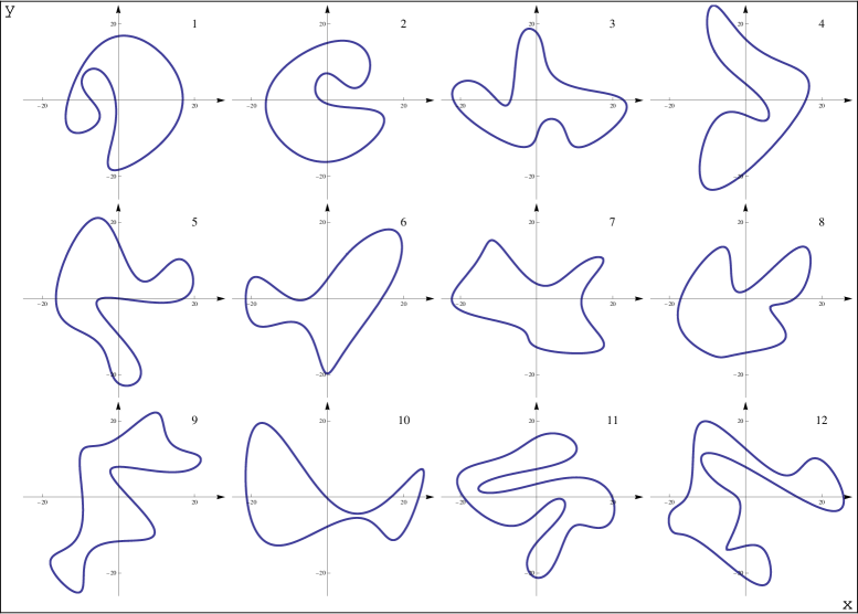
Figure 4.1: Initial curves contributing to the ensembles $E_{M}$. The positions of the ‘center of mass’ coincide with the origin, and all curves have the same area $200\,\pi$.

In Fig. 4.2, the evolution of two different initial curves under curve shrinking is shown.

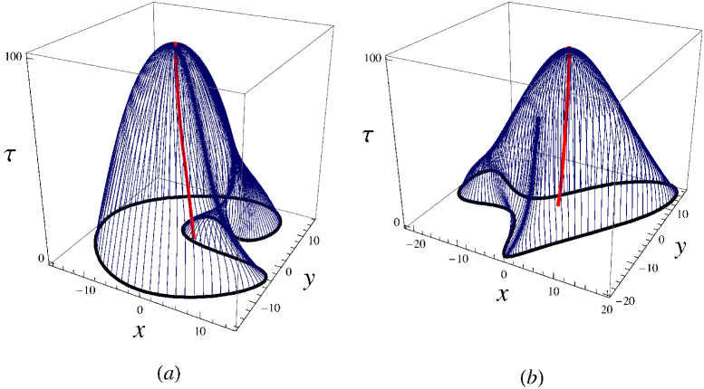
Figure 4.2: Plots of the evolution of planar N=0 CVLs (curve 2 and 6 of Fig. 4.1) under the curve shortening flow. The thick central lines depict the trajectories of the ‘center of mass’ (see Sec. 4.2.4) which coincides with the origin at $\tau=0$. The flow is started at $\tau=0$ and stopped at $\tau=100$.

4.2.2 Numerical procedure

The initial curves depicted in 4.1 are generated as follows. First, we chose a list of points in the $x\text{-}y$ plane such that the initial curve $\mathbf{x}(u,\tau=0)$ consecutively passes the points, where initial and final point coincide. A spline, which is made of piecewise third-order polynomials with $C^{1}$ continuity, interpolates each point in the list. Since Mathematica’s SplineFit sets the second derivatives of the spline at the endpoints to zero, the first two points are appended to the end of the list. The analogue holds for the last two points of the original list. To yield a smooth curve with more than $C^{1}$ continuity each coordinate of the curve is fitted by trigonometric functions up to order eight in its Fourier-expansion. Area, length and centroid of the initial curve are computed numerically with NIntegrate, where the latter is given by

$$\mathbf{x}_{\mbox{\tiny COM}}=\frac{1}{L}\int_{0}^{2\pi}\mathrm{d}u\,\left|\partial_{u}\mathbf{x}\right|\,\mathbf{x}.$$ (4.13)

Now we can prepare the ensembles as described in Sec. 4.2.1.

To simulate the flow evolution of the initial curves one searches for solutions to the second-order partial differential equation

$$\partial_{\tau}\mathbf{x}(u,\tau)=\frac{1}{|\partial_{u}\mathbf{x}(u,\tau)|}\partial_{u}\frac{1}{|\partial_{u}\mathbf{x}(u,\tau)|}\partial_{u}\mathbf{x}(u,\tau)$$ (4.14)

subject to periodic boundary conditions in the curve parameter, $\mathbf{x}(u=0,\tau)=\mathbf{x}(u=2\pi,\tau)$, and for the initial conditions $\mathbf{x}(u,\tau=0)$ depicted in Fig. 4.1. This is done using the Numerical Method of Lines. This is a technique for solving PDEs by discretizing in all but one dimension, and then integrating the semi-discrete problem as a system of coupled ordinary differential equations (ODEs) or differential-algebraic equations. Here, we partially discretize the flow equation Eq. (4.14) on a uniform grid in the parameter $u$ yielding an ODE initial value problem in $\tau$ that was solved by the ODE integrators in Mathematica’s NDSolve. Fig. 4.2 indicates why this technique is called the method of lines. As one can also see from Fig. 4.2, a set of discrete points on the curve, although remaining equidistant in $u$, may evolve under the flow such that the spatial distances between adjacent points falls below the numerical precision. The flow then encounters a purely numerically and thus virtual singularity (not to be confused with the earlier mentioned non-virtual singularities at $\tau=T$). Therefore, the execution of NDSolve is broken up into several basic steps which are carried out separately. These steps are:

(i) equation processing and method selection,

(ii) method initialization,

(iii) numerical solution,

(iv) solution processing.

The low-level functions that are used in Mathematica to break up these steps are NDSolve`ProcessEquations (i,ii), NDSolve`Iterate (iii) and NDSolve`ProcessSolutions (iv). NDSolve`ProcessEquations classifies the differential system into an initial-value problem, boundary-value problem, differential-algebraic problem, partial-differential problem, etc. It also chooses appropriate default integration methods and constructs the main NDSolve`StateData data structure. NDSolve`Iterate advances the numerical solution. The first invocation initializes the numerical integration methods. NDSolve`ProcessSolutions converts numerical data into an InterpolatingFunction to represent each solution. More precisely, the curve parameter range is divided into $n$ equidistant intervals yielding $n$ points on the curve which are generally not equidistant in space. For our simulation the number of points $n$ is chosen between 130 and 300. The discretization of flow equation (4.14) with respect to the variable $u$ needs to convert the derivatives into finite differences. The second-order centered (with respect to to the set of sample points around $x(u_{i})$) formula for the first derivative is given by

$$x^{\prime}(u_{i})=\frac{x(u_{i+1})-x(u_{i-1})}{2h}+\mathrm{O}(h^{2}),$$ (4.15)

where $h$ is the grid spacing. Here, finite differences of sixth order are used which are computed with Mathematica’s NDSolve`FiniteDifferenceDerivative. In the following, every quantity involving derivatives evaluated on a discrete set of data points is computed using Mathematica’s NDSolve`FiniteDifferenceDerivative. After NDSolve`ProcessEquations is invoked the first time at $\tau=\tau_{1}=0$, the numerical solution is advanced using NDSolve`Iterate by a unit ‘time’ step $\Delta\tau=1$ up to $\tau_{2}$. Then the computation is interrupted to compute an error estimate that indicates whether a virtual singularity is starting to evolve. The error estimate exploits that $A(\tau)=A_{0}-2\pi\,\tau$ and is computed as

$$10^{4}\times(A(\tau_{2})-A(\tau_{1})+2\pi(\tau_{2}-\tau_{1})),$$ (4.16)

where $A(\tau)$ is given by the discrete version of Eq. (3.14) evaluated on the point grid given by NDSolve.

Until $\tau_{2}$ reaches $T$, the solution is advanced step by step as long as the error estimate does not exceed the empirically found value of 2. But if it does, the by then obtained solution is fitted at $\tau_{2}-1$ in such a way that a new discretization yields (spatially) well separated points to restart the procedure. In Fig. 4.2(b) such a situation is shown. The fitted curve is obtained as follows. At $\tau_{1}$, one determines the minimal arc length $s_{\mathrm{min}}$ which is the least of all arc length between adjacent points on the curve. Then, at $\tau_{2}-1$, all those points on the curve are dropped the arc length of which to their next neighbors is less than the minimal arc length $s_{\mathrm{min}}$. The remaining points are fitted by trigonometric functions, where the order of the fit is chosen to depend on $\tau$ (since the curve is getting smoother with increasing $\tau$). In the case of the error estimate of the fitted curve exceeding the tolerance, the number of grid points has to be increased or the initial curve needs to be smoothed slightly. In order to avoid discontinuities in the $\tau$-evolution of $L$, $A$ and $x_{\mbox{\tiny COM}}$, and singularities in their derivatives that occur since the fit procedure generates piecewise defined functions, and since after the fit the values of $A$ and $L$ slightly deviate from their former values, these quantities are interpolated by polynomials for $0\leq\tau\leq T$ using FindFit. To improve the accuracy of $L$ near the critical value $T$, the isoperimetric ratio $\frac{L^{2}}{A}$ is fitted instead of $L$, and $L$ is calculated from $\sqrt{\left(\frac{L^{2}}{A}\right)_{\mbox{\tiny fitted}}\cdot A}$.

The analytical results of Sec. 3.1 such as the convergence of $\frac{L^{2}}{A}$ to $4\pi$, the constancy of $\dot{A}$ or the vanishing of $L$ and $A$ for $\tau\nearrow T$ are numerically well reproduced, thereby confirming the validity of the simulation.

The implicit first-order differential equation $\frac{\mathrm{d}Z}{\mathrm{d}\tau}=0$ for the coefficient is solved using NDSolve. If not set at will, the initial condition $c_{0}$ for $c(\tau)$ was derived from Eq. (4.12) using Mathematica’s FindRoot. The variance of the position of COM was computed. The square of the coefficient $c(\tau)$ associated to the non-conformal factor was fitted with function

$$c(\tau)^{2}=k(T_{0}-\tau)^{\alpha},$$ (4.17)

where $k$ and $\alpha$ are fit parameters. We have determined the critical exponent of the coefficient to $\frac{\alpha}{2}=0.5$ as $\tau\rightarrow T$, in accordance with the theoretical value of Eq. 4.7. For checking purpose, we have also used $T_{0}$ as fit parameter, yielding excellent agreement within the numerical precision.

A CD-ROM containing the used Mathematica notebooks is attached to the thesis.

4.2.3 Renormalization-group invariance of partition function

The function $c_{M}^{2}(\tau)$ is plotted in Fig. 4.3. According to Fig. 4.3 it seems that the larger the ensemble the closer $c_{M}^{2}(\tau)$ is to the evolution of a single circle of initial radius $R=\sqrt{\frac{A_{0}}{\pi}}$. For growing $M$ the function $c_{M}^{2}(\tau)$ approaches the form

$$c^{2}_{\mbox{\tiny as},M}(\tau)=k_{M}(T-\tau)\,,$$ (4.18)

where the slope $k_{M}$ depends on the strength of deviation from circles of the representatives in the ensemble $E_{M}$ at $\tau=0$, that is, on the variance $\Delta L_{M}$ at a given value $A_{0}$. Physically speaking, the value $\tau=0$ is associated with a certain initial resolution of the measuring device (the strictly monotonic function $\tau(Q)$, $Q$ being a physical scale such as energy or momentum transfer, expresses the characteristics of the measuring device and the measuring process), the value of $A_{0}$ describes the strength of noise associated with the environment ($A_{0}$ determines how fast the conformal limit of circular points is reached), and the values of $c_{0,M}$ and $k_{M}$, see Eq. (4.18), are associated with the conditions at which the to-be-coarse-grained system is prepared. Notice that this interpretation is valid for the ‘action’

$$S_{M}=\frac{L(\tau)^{2}}{A(\tau)}\left(1+\frac{c_{M}(\tau)}{L(\tau)}\right)$$

only.

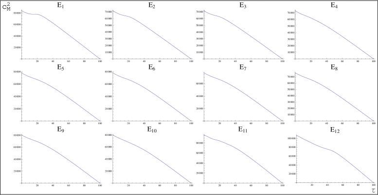
Figure 4.3: The square of the coefficient $c_{M}(\tau)$ entering the effective ‘action’ $S_{M}=\frac{L(\tau)^{2}}{A(\tau)}\left(1+\frac{c_{M}(\tau)}{L(\tau)}\right)$ for various ensemble sizes $M=1,\dots,12$. Notice the early onset of the linear drop of $c^{2}_{M}(\tau)$. The slope of $c^{2}_{M}(\tau)$ near $\tau=T$ does not depend on $c_{0,M}^{2}\equiv c^{2}_{M}(\tau=0)$ and thus not on the initial choice of $\bar{L}$, but only on the specific choice of curves included in the ensemble.

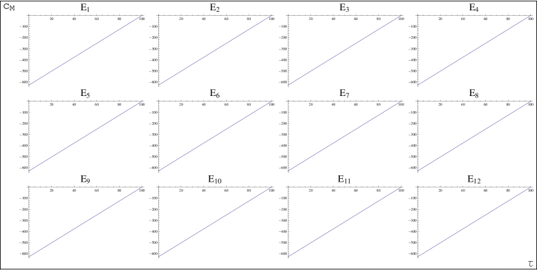
Figure 4.4: The coefficient $c_{M}(\tau)$ entering the effective ‘action’ $S_{M}=\frac{L(\tau)^{2}}{A(\tau)}\left(1+\frac{c_{M}(\tau)}{A(\tau)}\right)$ for ensemble sizes $M=1,\dots,12$.

If we relax initial condition $\bar{L}_{M}(0)=\tilde{L}_{M}(0)$ for $c_{0,M}$ and set the initial value for $c_{0,M}$ at will, the coefficient starts at the given value and rapidly adapts to the evolution depicted in Fig. 4.3 and respectively, Fig. 4.4. In Sec. 4.1.2, we have argued that for the modified ‘action’ and the initial condition $\bar{L}_{M}(0)=\tilde{L}_{M}(0)$ the curves are uniformly distributed. Relaxing this initial condition in the case of the modified ‘action’, means that the curves are no longer uniformly distributed for $\tau=0$. However, the uniform distribution is restored rapidly as the curves evolve under the flow.

4.2.4 Variance of mean ‘center of mass’

Having obtained the coefficient in the non-conformal factor of the effective ‘action’, we are now able to compute the flow of an ‘observable’, such as the COM position in a given ensemble and its statistical variance. The COM position $\mathbf{x}_{\mbox{\tiny{COM}}}$ of a given curve $\mathbf{x}(s,\tau)$ is defined as

$$\mathbf{x}_{\mbox{\tiny COM}}(\tau)=(x_{\mbox{\tiny COM}}(\tau),y_{\mbox{\tiny COM}}(\tau))^{T}=\frac{1}{L(\tau)}\int_{0}^{L(\tau)}\mathrm{d}s\,\mathbf{x}(s,\tau)\,.$$ (4.19)

We will present below results on the statistical variance of the COM position.

At $\tau=0$, the statistical variance in the position of the COM is prepared to be nil, physically corresponding to an infinite resolution applied to the system by the measuring device. In Fig. 4.5, the flow of the COM position corresponding to the initial curves depicted in Fig. 4.1 is shown.

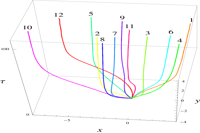
Figure 4.5: Flow of the positions of the ‘centers of masses’ for the initial curves depicted in Fig. 4.1.

The mean COM position $\bar{\mathbf{x}}_{\mbox{\tiny COM}}$ over the ensemble $E_{M}$ is defined as

$$\bar{\mathbf{x}}_{\mbox{\tiny COM}}(\tau)=(\bar{x}_{\mbox{\tiny COM}}(\tau),\bar{y}_{\mbox{\tiny COM}}(\tau))^{T}\equiv\frac{1}{Z_{M}}\sum_{i=1}^{M}\mathbf{x}_{\mbox{\tiny COM},i}(\tau)\exp\left(-S_{M}[\mathbf{x}_{i}(\tau)]\right)\,.$$ (4.20)

The scalar statistical deviation $\Delta_{M,\mbox{\tiny COM}}$ of $\bar{\mathbf{x}}_{\mbox{\tiny COM}}$ over the ensemble $E_{M}$ is defined as

$$\Delta_{M,\mbox{\tiny COM}}(\tau)\equiv\sqrt{\mbox{var}_{M,\mbox{\tiny COM};x}(\tau)+\mbox{var}_{M,\mbox{\tiny COM};y}(\tau)}\,,$$ (4.21)

where

$$\mbox{var}_{M,\mbox{\tiny COM};x} \equiv \frac{1}{Z_{M}}\sum_{i=1}^{M}\left(x_{\mbox{\tiny COM},i}(\tau)-\bar{x}_{\mbox{\tiny COM}}(\tau)\right)^{2}\,\exp\left(-S_{M}[\mathbf{x}_{i}(\tau)]\right)$$ (4.22)

$$= -\bar{x}^{2}_{\mbox{\tiny COM}}(\tau)+\frac{1}{Z_{M}}\sum_{i=1}^{M}x^{2}_{\mbox{\tiny COM},i}(\tau)\,\exp\left(-S_{M}[\mathbf{x}_{i}(\tau)]\right),$$

and similarly for the coordinate $y$. In Fig. 4.6, plots of $\Delta_{M,\mbox{\tiny COM}}(\tau)$ are shown when $\Delta_{M,\mbox{\tiny COM}}(\tau)$ is evaluated over the ensembles $E_{1},\dots,E_{12}$ with the ‘action’

$$S_{M}=\frac{L(\tau)^{2}}{A(\tau)}\left(1+\frac{c_{M}(\tau)}{L(\tau)}\right)$$

and subject to the initial condition $\bar{L}_{M}(\tau=0)=\tilde{L}_{M}(\tau=0)$. In Fig. 4.7, the according plots of $\Delta_{M,\mbox{\tiny COM}}(\tau)$ are depicted as obtained with the modified ‘action’

$$S_{M}=\frac{L(\tau)^{2}}{A(\tau)}\left(1+\frac{c_{M}(\tau)}{A(\tau)}\right)$$

and subject to the initial condition $\bar{L}_{M}(\tau=0)=\tilde{L}_{M}(\tau=0)$. In this case, one has $c_{M}(\tau)=-A(\tau)$ leading to equal weights for each curve in $E_{M}$.

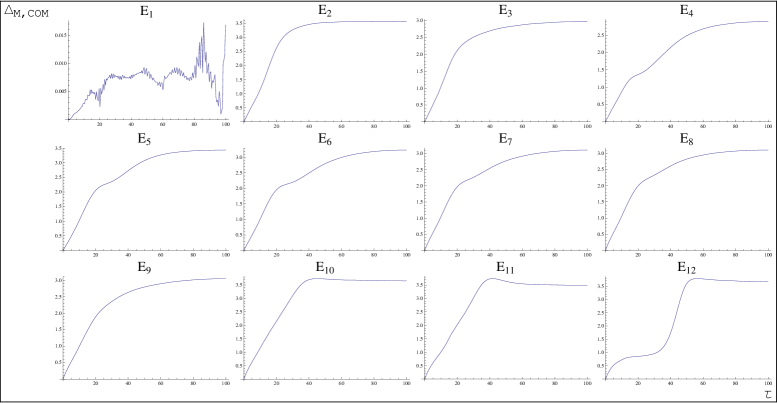
Figure 4.6: Plots of $\Delta_{M,\mbox{\tiny COM}}(\tau)$ for $M=1,\dots,12$ when evaluated with the ‘action’ $S_{M}=\frac{L(\tau)^{2}}{A(\tau)}\left(1+\frac{c_{M}(\tau)}{L(\tau)}\right)$. Notice the rapid generation of an uncertainty in the COM position under the flow and its saturation when approaching the conformal limit $\tau\nearrow T$. There also is a saturation of this limiting value with a growing ensemble size.

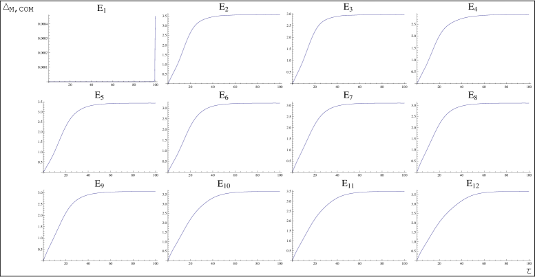
Figure 4.7: Plots of $\Delta_{M,\mbox{\tiny COM}}(\tau)$ for $M=1,\dots,12$ when evaluated with the modified ‘action’ $S_{M}=\frac{L(\tau)^{2}}{A(\tau)}\left(1+\frac{c_{M}(\tau)}{A(\tau)}\right)$. This corresponds to a uniform distribution when evaluated with initial condition (4.12). Notice the qualitative agreement with the results displayed in Fig. 4.6.

Note that the slight qualitative deviation of the last graph $E_{12}$ for small values of $\tau$ regarding to the previous graphs in Fig. 4.6 is due to the fact that the curves which were added to the ensemble at last are the most twisted ones. Graph $E_{12}$ still saturates at a finite value of $\tau$, nevertheless. The fluctuations in graph $E_{1}$ of Fig. 4.6 are within the range of the numerical precision.

4.2.5 Quantum mechanical versus statistical uncertainty

In view of the results obtained in the last section, we would say that an ensemble of evolving planar CVLs in the $N=0$ sector qualitatively resembles the Quantum Mechanics of a free point particle of mass $m$ in one space dimension $x$. Namely, an initially localized square of the wave function $\psi$ with $|\psi(\tau=0,x)|^{2}\propto\exp\left[-\frac{x^{2}}{a_{0}^{2}}\right]$, where $\Delta x(\tau=0)=a_{0}$, according to unitary time evolution in quantum mechanics evolves as

$$|\psi(\tau,x)|^{2}=|\exp\left[-\mathrm{i}\frac{H\tau}{\hbar}\right]\psi(\tau=0,x)|^{2}\propto\exp\left[-\frac{(x-\frac{p}{m}\tau)^{2}}{a^{2}(\tau)}\right],$$ (4.23)

where $H=\frac{p^{2}}{2m}$ is the free-particle Hamiltonian, $p$ the spatial momentum, and $a(\tau)\equiv a_{0}\sqrt{1+\left(\frac{\hbar\tau}{ma_{0}^{2}}\right)^{2}}$. In agreement with Heisenberg’s uncertainty relation, one has during the evolution that

$$\Delta x\Delta p=\frac{\hbar}{2}\sqrt{1+\left(\frac{\tau\hbar}{ma_{0}^{2}}\right)^{2}}\geq\frac{\hbar}{2}.$$ (4.24)

The time evolution in a quantum mechanical system and the process of lowering the resolution in a statistical system describing planar CVLs share the same property: the ‘time’ (resolution) evolution generates out of a small initial position uncertainty (corresponding to a large initial resolution $\Delta p$) a larger position uncertainty as ‘time’ increases (resolution decreases). Possibly, future development will show that interference effects in Quantum Mechanics can be traced back to the non-local nature of the degrees of freedom (CVLs) entering a statistical partition function.

Chapter 5 Selfintersecting center-vortex loops

Let us now turn to the case of $N=1$ CVLs. We proceed as far as possible in close analogy to the $N=0$ sector.

5.1 Wilsonian renormalization-group flow

5.1.1 Geometric partition function

As in the $N=0$ sector, we interpret curve-shrinking as a Wilsonian renormalization-group flow. The partition function is now defined over an ensemble of $N=1$ CVLs, and we consider it to be independent under a change of resolution $Q$ and thus independent of $\tau$. We express the effective ‘action’ in terms of integrals over local densities in $s$, and demand the following symmetries in order to conceive an ansatz for the effective ‘action’:

(i) scaling symmetry $\mathbf{x}\to\lambda\mathbf{x}\,,\ \lambda\in{\mathbb{R}}_{+}$: for $\lambda\to\infty$, implying $\lambda L\to\infty$ at fixed $L$, the ‘action’ $S$ should be invariant under further finite rescalings (decoupling of the fixed length scales $\sigma^{-1/2}$ and $\Lambda^{-1}$).

(ii) Euclidean point symmetry of the plane: this is sufficiently satisfied for a representation of $S$ in terms of integrals over scalar densities with respect to these symmetries. Thus, we can represent the ‘action’ density as a series involving products of Euclidean scalar products of $\frac{\partial^{n}}{\partial s^{n}}\mathbf{x}\,,\ n\in\mathbb{N}_{+}\,,$ or constancy.

As in Sec. 4.1.1, we resort to a factorization ansatz as

$$S=F_{c}\times F_{nc},$$ (5.1)

where in addition to Euclidean point symmetry $F_{c}$ ($F_{nc}$) is (is not) invariant under $\mathbf{x}\to\lambda\mathbf{x}$. In principle, infinitely many operators can be defined to contribute to $F_{c}$. Since the evolution homogenizes the curvature, except for a small vicinity of the intersection point where one or both loops of the curve vanish, higher derivatives of $k$ with respect to $s$ should not be of importance. This should also hold for Euclidean scalar products involving higher derivatives $\frac{\partial^{n}}{\partial s^{n}}\mathbf{x}$. Conformally invariant expressions are obtained from such integrals if multiplied by powers of $\sqrt{A}$ and/or $L$ or the inverse of integrals involving lower derivatives. The conformal factor $F_{c}$ is set equal to the isoperimetric ratio,

$$F_{c}(\tau)\equiv\frac{L(\tau)^{2}}{A(\tau)}\,.$$ (5.2)

The property of conformal invariance for $L,A\to\infty$ suggests to express the non-conformal factor $F_{nc}$ as a formal expansion in inverse powers of $L$ or $A\equiv A_{1}+A_{2}$. We allow for an explicit $\tau$ dependence of the coefficient $c$ of the lowest nontrivial power $\frac{1}{L}$ or $\frac{1}{A}$. In principle, this sums up the contribution to $F_{nc}$ of certain higher-power operators which do not exhibit an explicit $\tau$ dependence.

We restrict to the following two ansätze for the non-conformal factor in Eq. (5.1),

$$F_{nc}(\tau)=1+\frac{c(\tau)}{L(\tau)}\,.$$ (5.3)

and for the modified ‘action’

$$F_{nc}(\tau)=1+\frac{c(\tau)}{A(\tau)}\,.$$ (5.4)

The initial value $c(\tau=0)$ is determined from the physical boundary condition such as the mean length $\bar{L}$ at $\tau=0$. Although the modified ansatz (5.4) in $F_{nc}$ of the geometric ‘action’ is profoundly different physical results such as the evolution of entropy or the variance of intersection of a given ensemble agree remarkably well, see Sec. 5.2

5.1.2 Effective ‘action’

The effective ‘action’ $S_{M}[\mathbf{x}(\tau)]$ results from a partition function $Z_{M}$ which is defined as the average

$$Z_{M}=\sum_{i}^{M}\exp\left(-S_{M}[\mathbf{x}_{i}(\tau)]\right)$$ (5.5)

over the nontrivial ensemble $E_{M}=\{\mathbf{x}_{1},\dots\,\mathbf{x}_{M}\}$. The ensemble $E_{M}$, consisting of $M$ curves, is obtained from $E_{M-1}$ by adding a new curve $\mathbf{x}_{M}(\tau)$. The effective ‘action’ $S_{M}$ in Eq. (5.1) is determined by the function $c_{M}(\tau)$, the flow of which follows from the requirement of $\tau$-independence of the partition function:

$$\frac{\mathrm{d}}{\mathrm{d}\tau}Z_{M}=0.$$ (5.6)

As in Sec. 4.1.2, we obtain the initial condition $c_{0,M}=c_{M}(\tau=0)$ to this implicit first-order ordinary differential equation by the constraint that the geometric mean coincides with the statistic mean at $\tau=0$,

$$\bar{L}_{M}(0)=\tilde{L}_{M}(0).$$ (5.7)

5.2 Results of simulation

5.2.1 Preparation of ensembles

Similar to Sec. 4.2.1, all curves are normalized curves to have the same initial total area $A_{0}=A_{0,1}+A_{0,2}$ and since we are now interested in the position of the intersection where the (anti)monopole is localized (see Sec. 2.4 or Fig. 6.1), we have applied a translation to each curve in the ensemble $E_{M}$ such that the location of the intersections initially coincide with the origin. Again, such a transition does not alter the effective ‘action’ due to Euclidean point symmetry.

We order the members of the maximal-size ensemble $E_{M=16}$ into sub-ensembles $E_{M<16}$ such that $T_{i=1}\geq T_{i=2}\geq\dots\geq T_{M}$, because the critical value $T$ of the flow parameter $\tau$ varies from curve to curve. These ensembles $E_{M}$ are referred to as $T$-ordered. We have also performed all simulations with ensembles $E^{\prime}_{M<16}$ the members of which are picked randomly from $E_{M=16}$ and have obtained similar results for ensemble averages of ‘observables’ using $E_{M<16}$ and $E^{\prime}_{M<16}$ for the $\tau$ evolution to the left of $\tau=\min\{T_{i}|\mathbf{x}_{i}\in E^{\prime}_{M<16}\}$. The main difference is that the computation of the coefficient, and with it the flow of ‘observables’, terminates at a smaller $\tau$ since the ensembles $E^{\prime}_{M}$ are no longer $T$-ordered.

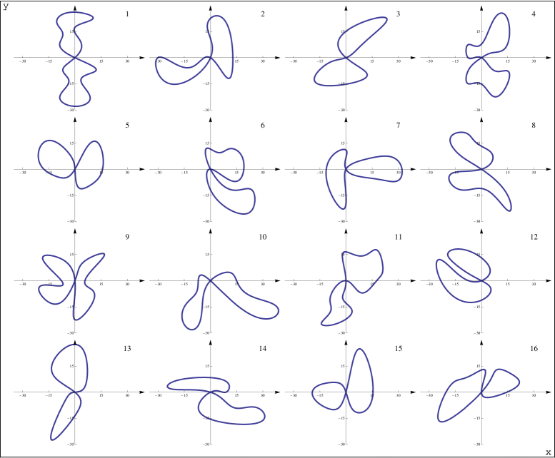
Figure 5.1: Initial curves $\mathbf{x}_{i}(u,\tau=0)$ contributing to the ensemble $E_{M=16}$. The intersection points $x_{{\mbox{\tiny int}},i}(\tau=0)$ coincide with the origin, and all curves have the same area $200\,\pi$. By definition $E_{M=16}$ is $T$-ordered.

The maximal-size ensemble $E_{M=16}$ at $\tau=0$ is depicted in Fig. 5.1 with the universal choice $A_{0}=200\,\pi$. The curves in Fig. 5.1 are arranged in a $T$-ordered way. We have $T_{i=1}=65\geq T_{2}\geq\dots\geq T_{M}=43$. In Fig. 5.2, the evolution of an initial curve (number 12 of Fig. 5.1) under curve shrinking is shown from two points of view. The flow is started at $\tau=0$ and stopped at a value of $\tau$ shortly below $T$.

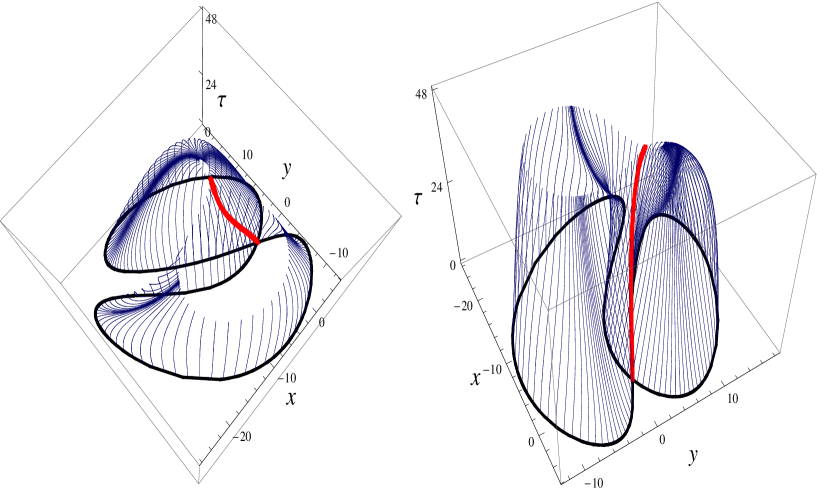
Figure 5.2: Plots of the evolution of an $N=1$ center-vortex loop (curve 12 of Fig. 5.1) under curve shrinking. The thick central line depicts the trajectory of the intersection point which coincides with the origin at $\tau=0$.

In Fig. 5.3, the flow of the intersection points $\mathbf{x}_{\mbox{\tiny int},i}(\tau)$ corresponding to the initial curves depicted in Fig. 5.1 is shown.

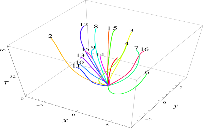
Figure 5.3: Flow of the intersection points $\mathbf{x}_{{\mbox{\tiny{int}}},i}(\tau)$ for the initial curves depicted in Fig. 5.1.

5.2.2 Numerical investigation

In general, the procedure is in close analogy to Sec. 4.2.2. Therefore, we solely mention the differences compared to Sec. 4.2.2. The choice of sample points, used to generate the initial curves, is now done in such a way that, if interpolated one after another by a cubic spline with coinciding initial and end point, the curve will cross itself once. The number of grid points $n$ is set to 300 for all curves, except for curve 9 where 500 points are used. For the simplicity of the computation of the intersection of the initial curve, the intersection point is included in the set of sample points as a double point and is chosen to coincide with the origin.

The search for solutions to the flow equation is proceeded as in Sec. 4.2.2 using the Numerical Method of Lines. Starting from $\tau=\tau_{1}=0$ the solution is advanced step by step as long as $\tau<T$ or a virtual singularity evolves. If the latter is the case we start the same fitting procedure as in Sec. 4.2.2. The error estimate of Sec. 4.2.2, based on the constant value of $\dot{A}$, is no longer applicable in the case of selfintersecting curves, however, $\Delta A(\tau)=A_{1}(\tau)-A_{2}(\tau)=\mathrm{constant}$ can serve to estimate a value that indicates the validity of the numerical solution. The error estimate is defined as

$$10^{6}\times\left(1-\frac{\Delta A(\tau)}{\Delta A(\tau_{1})}\right).$$ (5.8)

In the case where both areas of the curve have almost the same value, and the absolute of $A$ falls below the numerical precision, we have used

$$10^{6}\times(\Delta A(\tau_{1})-\Delta A(\tau)).$$ (5.9)

Since Eq. (3.27) involves the two-dimensional curl the straight forward discretization of this equation already computes the (signed) difference $\Delta A$ of the areas enclosed by the curve. Therefore, we do not have to keep track of the selfintersection during the numerical evolution of the curve. However, the computation of the total area involves knowledge of $A_{1}$ and $A_{2}$, and this in turn of the intersection point. Once the error estimate exceeds a value of 2 the curve is fitted to yield again spatially well separated points. We also used the error estimate to recognize the final (non-virtual) singularity at $T$, where a further evolution in the sense of the flow equation is impossible and does not make sense.

To compute the position of intersection point one searches, at a first step, for those two points in the solution set at given $\tau$ which are spatially nearest to each other, but with the restriction that they are element of different line segments of the curve which generate the intersection point. Therefore, the spatial distances between the $i^{th}$ and $j^{th}$ point on the curve are determined for all pairs of points with $|i-j|>d_{\mathrm{min}}$, where $d_{\mathrm{min}}$ depends on the considered curve and has to be adjusted for each individually. Then it is searched for the least of all distances to find that pair of points which is closest to the intersection point. The minimal distance of indices $d_{\mathrm{min}}$ is introduced because, as the flow evolves the curve, next neighboring points could become (spatially) closer to each other than the points nearest to the intersection. Once the pair of points which is next to the intersection is found, the two curve segments around these points are approximated by cubic splines. Now the intersection of these two splines is computed using Mathematica’s FindRoot

At given $\tau$, length and area of the curves are computed with their discrete formulas using Mathematica’s FiniteDifferenceDerivative. For the same reasons as in Sec. 4.2.2 the $\tau$-evolution of $L$, $A$ and $\mathbf{x}_{\mbox{\tiny int}}$ are interpolated by polynomials.

Finally, the implicit first-order differential equation $\mathrm{d}Z/\mathrm{d}\tau=0$ for the coefficient is solved using NDSolve for all ensembles sizes and orderings and for both ‘actions’. If not set at will, the initial condition $c_{0}$ for $c(\tau)$ was derived from Eq. (5.7) using Mathematica’s FindRoot. Variance of mean intersection and entropy were computed.

A CD-ROM containing the used Mathematica notebooks is attached to the thesis.

5.2.3 Renormalization-group invariance of partition function

We now present the results of the simulation. For all ensembles $E_{M}$, the $\tau$ dependence of the coefficient $c_{M}$ in Eq. (5.3) roughly behaves like a square root $\propto\sqrt{T_{M}-\tau}$ where $T_{M}$ is the weakly ensemble-dependent minimal resolution. For the modified ‘action’ $S_{M}=\frac{L(t)^{2}}{A(t)}\left(1+\frac{c_{M}(t)}{A(t)}\right)$ the coefficient $c_{M}(\tau)$ is well approximated by a linear function $\propto T_{M}-\tau$. Again, $T_{M}$ is a weakly ensemble-dependent minimal resolution. For $T$-ordered ensembles the results for $c_{M}(\tau)$ for the ‘actions’ Eq. (5.3) and Eq. (5.4) are shown in Fig. 5.4 and respectively, in Fig. 5.5. The results for the ensembles $E^{\prime}_{M}$ do not differ sizably from those presented in Fig. 5.4 and respectively, in Fig. 5.5.

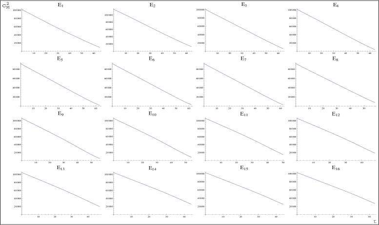
Figure 5.4: The squares of the coefficients $c_{M}(\tau)$ entering the ansatz for effective ‘action’ $S_{M}=\frac{L(\tau)^{2}}{A(\tau)}\left(1+\frac{c_{M}(\tau)}{L(\tau)}\right)$ for $T$-ordered ensembles up to $M=16$.

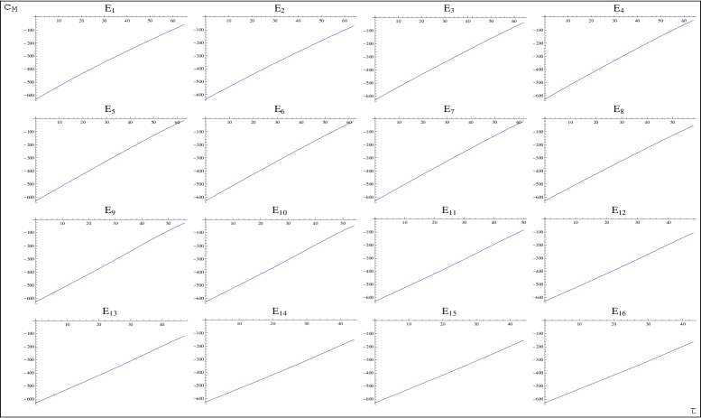
Figure 5.5: The coefficient $c_{M}(\tau)$ entering the ansatz for the effective ‘action’ $S_{M}=\frac{L(\tau)^{2}}{A(\tau)}\left(1+\frac{c_{M}(\tau)}{A(\tau)}\right)$ for $T$-ordered ensembles up to $M=16$.

5.2.4 Variance of location of selfintersection

The mean intersection $\bar{\mathbf{x}}_{\mbox{\tiny int}}(\tau)$ over the ensemble $E_{M}$ is defined as

$$\bar{\mathbf{x}}_{\mbox{\tiny int}}(\tau)=(\bar{x}_{\mbox{\tiny int}}(\tau),\bar{y}_{\mbox{\tiny int}}(\tau))^{T}\equiv\frac{1}{Z_{M}}\sum_{i=1}^{M}\mathbf{x}_{\mbox{\tiny int},i}(\tau)\exp\left(-S_{M}[\mathbf{x}_{i}(\tau)]\right)\,,$$ (5.10)

where $\mathbf{x}_{\mbox{\tiny int},i}(\tau)=(x_{\mbox{\tiny int}}(\tau),y_{\mbox{\tiny int}}(\tau))^{T}$ is the location of the point of selfintersection of curve $\mathbf{x}_{i}$ at $\tau$. The scalar statistical deviation $\Delta_{M,\mbox{\tiny int}}$ of $\bar{\mathbf{x}}_{\mbox{\tiny int}}$ over the ensemble $E_{M}$ is defined as

$$\Delta_{M,\mbox{\tiny int}}(\tau)\equiv\sqrt{\mbox{var}_{M,\mbox{\tiny int};x}(\tau)+\mbox{var}_{M,\mbox{\tiny int};y}(\tau)}\,,$$ (5.11)

where

$$\mbox{var}_{M,\mbox{\tiny int};x} \equiv \frac{1}{Z_{M}}\sum_{i=1}^{M}\left(x_{\mbox{\tiny int},i}(\tau)-\bar{x}_{\mbox{\tiny int}}(\tau)\right)^{2}\,\exp\left(-S_{M}[\mathbf{x}_{i}(\tau)]\right)$$ (5.12)

$$= -\bar{x}^{2}_{\mbox{\tiny int}}(\tau)+\frac{1}{Z_{M}}\sum_{i=1}^{M}x^{2}_{\mbox{\tiny int},i}(\tau)\,\exp\left(-S_{M}[\mathbf{x}_{i}(\tau)]\right)$$

and similarly for the coordinate $y$. In Fig. 5.6, plots of $\Delta_{M,\mbox{\tiny int}}(\tau)$ are shown when evaluated over the ensembles $E_{1},\dots,E_{16}$ subject to the ‘action’

$$S_{M}=\frac{L(\tau)^{2}}{A(\tau)}\left(1+\frac{c_{M}(\tau)}{L(\tau)}\right)$$

and the initial condition $\bar{L}_{M}(\tau=0)=\tilde{L}_{M}(\tau=0)$. In Fig. 5.7, the according plots of $\Delta_{M,\mbox{\tiny int}}(\tau)$ are depicted as obtained with the ‘action’

$$S_{M}=\frac{L(\tau)^{2}}{A(\tau)}\left(1+\frac{c_{M}(\tau)}{A(\tau)}\right)$$

and subject to the initial condition $\bar{L}_{M}(\tau=0)=\tilde{L}_{M}(\tau=0)$.

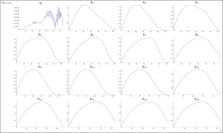
Figure 5.6: Plots of $\Delta_{M,\mbox{\tiny int}}(\tau)$ for the $T$-ordered ensembles $E_{M}$ with $M=1,\dots,16$. We have employed the ansatz for the ‘action’ $S_{M}=\frac{L(\tau)^{2}}{A(\tau)}\left(1+\frac{c_{M}(\tau)}{L(\tau)}\right)$.

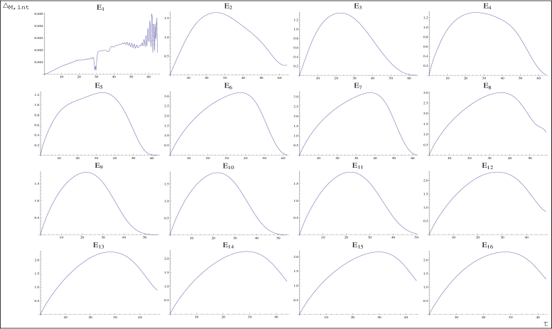
Figure 5.7: Plots of $\Delta_{M,\mbox{\tiny int}}(\tau)$ for the $T$-ordered ensembles $E_{M}$ with $M=1,\dots,16$. We have employed the ansatz for the modified ‘action’ $S_{M}=\frac{L(\tau)^{2}}{A(\tau)}\left(1+\frac{c_{M}(\tau)}{A(\tau)}\right)$.

Relaxing the constraint of $T$-ordering ($E_{M}\to E^{\prime}_{M}$) does not entail a qualitative change of the results. The fluctuation in the first graph of Fig. 5.6 and in Fig. 5.7, representing the trivial ensemble $E_{M=1}$ is within the range of the numerical precision. The results presented in Fig. 5.6 and Fig. 5.7 are unexpected since in the $N=0$ sector the variance of the ‘center of mass’ saturates rapidly to finite values. In contrast, for the $N=1$ sector, the variance of the location of selfintersection initially increases, reaches a maximum, and decreases to zero at a finite value of $\tau$. This is readily confirmed by the evaluation of the entropy, see next section.

5.2.5 Evolution of entropy

Let us now investigate the flow of entropy. The weight-functional $P_{M}$ is defined as

$$P_{M}(\tau)=P_{M}[\mathbf{x}_{{\mbox{\tiny int}},i}(\tau)]\equiv\frac{1}{Z_{M}}\exp({-S_{M}[\mathbf{x}_{i}(\tau)]}),$$ (5.13)

and the entropy $\Sigma_{M}$ as

$$\Sigma_{M}(\tau)=\Sigma_{M}[\mathbf{x}_{{\mbox{\tiny int}},i}(\tau)] \equiv \sum_{i=1}^{M}P_{M}[\mathbf{x}_{{\mbox{\tiny int}},i}(\tau)]\log\left(P_{M}[\mathbf{x}_{{\mbox{\tiny int}},i}(\tau)]\right)$$ (5.14)

$$= \log Z_{M}+\frac{1}{Z_{M}}\sum_{i=1}^{M}S_{M}[\mathbf{x}_{i}(\tau)]\,\exp\left(-S_{M}[\mathbf{x}_{i}(\tau)]\right)$$ (5.15)

where $S_{M}[\mathbf{x}_{i}(\tau)]$ is given by Eq. (5.1). In Figures 5.8 and 5.9, plots are shown for $\Sigma_{M}(\tau)$ when evaluated with the ‘action’

$$S_{M}=\frac{L(\tau)^{2}}{A(\tau)}\left(1+\frac{c_{M}(\tau)}{L(\tau)}\right)$$

and respectively, when evaluated with the modified ‘action’

$$S_{M}=\frac{L(\tau)^{2}}{A(\tau)}\left(1+\frac{c_{M}(\tau)}{A(\tau)}\right)$$

for $T$-ordered ensembles of size $M=1,\dots,16$.

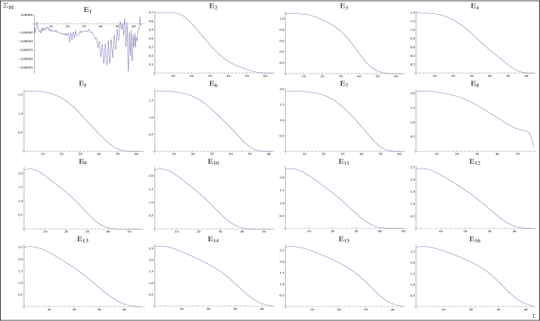
Figure 5.8: Flow of the entropies $\Sigma_{M}$ for $T$-ordered ensembles of size $M=1,\dots,16$ when evaluated with the ‘action’ $S_{M}=\frac{L(\tau)^{2}}{A(\tau)}\left(1+\frac{c_{M}(\tau)}{L(\tau)}\right)$.

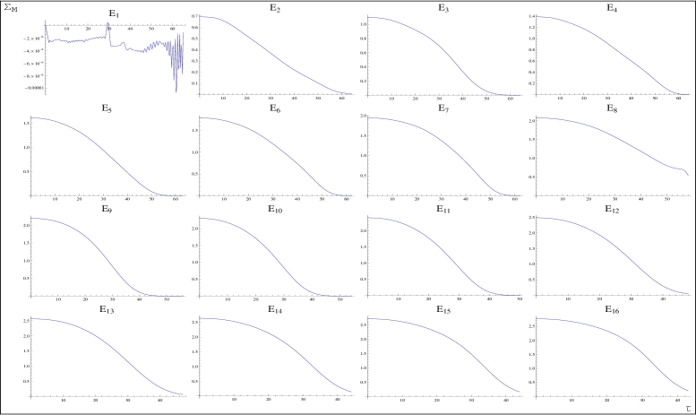
Figure 5.9: Flow of the entropies $\Sigma_{M}$ for $T$-ordered ensembles of size $M=1,\dots,16$ when evaluated with the modified ‘action’ $S_{M}=\frac{L(\tau)^{2}}{A(\tau)}\left(1+\frac{c_{M}(\tau)}{A(\tau)}\right)$.

The continuous approach of entropy to zero at finite values of $\tau$ implies the spontaneous emergence of order in the system as the resolution decreases: starting at a finite value of $\tau$, a particular member of $E_{M}$ is singled out by its weight approaching unity. This is validated by Fig. 5.10 where the weight-functionals $P_{M}$ are shown for $T$-ordered ensembles of size $M=2,\dots,4$. The pattern that a curve is singled out by its weight-functional as $\tau$ increases continues for all ensemble sizes $M$. In view of Chapter 4, this behavior is highly unexpected and we conclude that the nontrivial topology of the $N=1$ sector induces qualitative differences into the coarse-graining process.

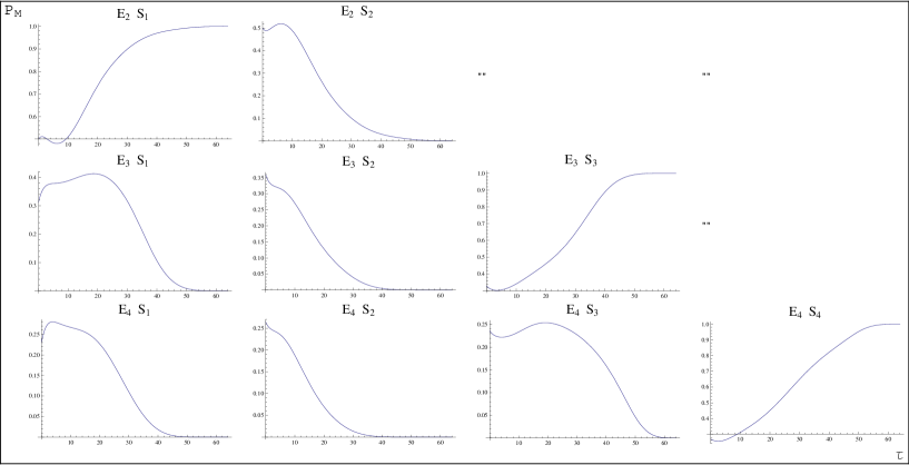
Figure 5.10: Weights $\frac{1}{Z_{M}}e^{-S_{M}[\mathbf{x}_{i}(\tau)]}$ of the curves $\mathbf{x}_{i}$ for $i=1,\dots,M$ and for $T$-ordered ensembles of size $M=2,\dots,4$ when evaluated with the ‘action’ $S_{M}=\frac{L(\tau)^{2}}{A(\tau)}\left(1+\frac{c_{M}(\tau)}{L(\tau)}\right)$.

Chapter 6 Applications

Here, it should be recalled that a magnetic charge emerging as a result of the dynamically broken gauge-symmetry SU(2) $\rightarrow$ U(1) in the deconfining phase is interpreted as an electric charge with respect to the U(1)_Y subgroup of the electroweak sector. In view of Sec. 6.2, recall that the magnetic center flux of the confining SU(2)_e is dually interpreted as electric flux.

6.1 Solitonic fermions

The notion of a point-like electron has always been plagued by its diverging self-energy. Even in classical field theory it is present in the shape of the infinite self-energy of a point charge. If the electron is considered to be a little sphere of radius $R$ and mass $m_{e}$ with electric charge $e$ attached to the sphere, then the electric field energy $U$ is given by

$$U=\frac{e^{2}}{8\pi R}.$$ (6.1)

Sending $R$ to zero, as we have to if we think of the electron as a point particle, the self-energy contribution to the mass of the electron diverges. In Quantum Electrodynamics (QED), the problem persists: the correction to the electron mass is still infinite, although it has a much softer logarithmic divergence $(c=\hbar=1)$,

$$\delta m_{\mbox{\tiny QED}}=3\frac{e^{2}}{8\pi^{2}}\ln(m_{e}R).$$ (6.2)

Therefore, one needs to employ renormalization theory to cope with the emerging divergences that are to a large extent a direct consequence of locality: the point-particle like nature of the electron. “…, and despite the comparative success of renormalisation theory the feeling remains that there ought to be a more satisfactory way of doing things.” as Lewis Ryder put in [8].

In the Standard Model, the electron is represented by the famous Dirac equation. Though it successfully predicts the electron’s antiparticle, the positron, and the magnetic moment with an $g$-factor of 2 it has to introduce the concept of the Dirac sea to make sense of the infinite number of negative-energy eigenstates. The Dirac sea leads to an infinite contribution to the energy density of the ‘vacuum’ which has to be canceled, somehow. Furthermore, the Standard Model does not provide for a deeper explanation of the value of the magnetic dipole moment other than that following from the Dirac equation and small radiative corrections. Moreover, the electron mass enters the QED Lagrangian as a free parameter, and the running of which with resolution needs additional experimental input.

The excitations in the confining phase of SU(2) Yang-Mills thermodynamics are single and selfintersecting center-vortex loops. The mass of each intersection point in a selfintersecting center-vortex loop is given by the Yang-Mills scale $\Lambda_{c}$. Since a monopole (antimonopole) is located at the intersection, it carries one unit of electric charge. Recall that a magnetically charged object in the defining gauge theory has to be interpreted as an electrically charged object in the Standard Model - and vice versa. In a given segment of a flux tube, the monopoles (antimonopoles) can move in both directions: there is a two-fold degeneracy of direction of the center flux that is analogue to the two-fold degeneracy of the spin projection. Moreover, for each center-vortex loop it is possible to move along the entire flux system on a closed curve. Thus, the projection of the dipole moment generated by the current of monopoles and antimonopoles inside the vortex core onto a given direction in space is two-fold degenerated as well. Therefore, we identify each soliton with a spin-1/2 fermion. Setting the Yang-Mills scale $\Lambda_{C}$ equal to the electron mass $m_{e}$, we are led to interpret $N=1$ center-vortex loops as electrons or positrons [10, 16, 23].

Let us consider the process of twisting and charge localization more closely. The transition from a non-selfintersecting to selfintersecting center-vortex loop is by twisting of a non-selfintersecting curve. The emergence of a localized (anti)monopole in the process is due to its capture by oppositely directed center fluxes in the core of the intersection (eye of the storm). By a rotation of the left half-plane in Fig. 6.1(a) by an angle of $\pi$, see Fig. 6.1(b), each wing of the center-vortex loop forms a closed flux loop by itself, thereby introducing equally directed center fluxes at the intersection point.

Figure 6.1: (Topological) transition from the $N=0$ sector (a), (b), (c) to the $N=1$ sector (d) by twisting and subsequent capture of a magnetic (anti)monopole in the core of the final intersection. Arrows indicate the direction of center flux.

This does not allow for an isolation of a single spinning (anti)monopole in the core of the intersection and thus is topologically equivalent to the untwisted case Fig. 6.1(a). However, another rotation of the left-most half-plane in Fig. 6.1(c) introduces an intermediate loop which by shrinking is capable of isolating a spinning (anti)monopole due to oppositely directed center fluxes. Notice that in the last stage of such a shrinking process (short distances between the cores of the flux lines), where propagating dual gauge modes are available, there is repulsion due to Biot-Savart which needs to be overcome. This necessitates an investment of energy manifesting itself in terms of the mass of the isolated (anti)monopole (eye of the storm). Alternatively, the emergence of an isolated (anti)monopole is possible by a simple pinching of the untwisted curve, again having to overcome local repulsion in the final stage of this process.

In the analysis performed in Chapter 5, we have solely regarded the situation depicted in Fig. 6.1(d), since the direction of center flux within a given curve segment is irrelevant for the process of a spatial coarse-graining microscopically described by the same curve-shrinking flow as applied to $N=0$ center-vortex loops in Chapter 4.

There are also phenomenological reasons that argue for a non-local nature of the electron. Recall that the imaginary part of the pressure in the confining phase starts to dominate when approaching the Hagedorn transition, thereby inducing microturbulences in the plasma (see Sec. 2.4). Such a nonthermal behaviour is likely to be related to the observed but poorly understood microturbulences and internal transport barriers in tokamak experiments with magnetically confined plasma. This presumes to identify the neutrino and the electron with the non-selfintersecting and the one-fold selfintersecting center-vortex loop of the confining phase of SU(2)_e with Yang-Mills scale $\Lambda_{c}=m_{e}=511$ keV. Here, it should be noticed that due to the absence of an antiparticle in the case of a $N=0$ soliton neutrinos need to be of Majorana type which is in compliance with the successful search for the neutrinoless double $\beta$ decay [4].

This interpretation is also supported by recent high-temperature $Z$-Pinch experiments at Sandia National Laboratories detecting an unexpected powerful contained explosion. There, an electric current rises in a wire array up to $\sim 20$ MA within $\sim 100$ ns, thereby the wire is transformed into a plasma column. The strong magnetic field induced by the current results in an inward directed (magnetic) pressure $P_{m}$ which compresses the plasma until it collapses. In the course of the implosion, the ions and electrons are accelerated towards the plasma axis. The radiated soft x-ray energy is as much as four times the kinetic energy that is expected to be released by the intersection of ions and electrons. However, before the plasma explodes it stabilizes for about 5 ns (stagnation). The measured electron temperature $T_{e}$ is found to be $\sim 3$ keV at stagnation. Preceding the explosion, an ion temperature $T_{i}$ about $300$ keV is sustained shortly after the plasma has stagnated [15]. The outward directed plasma pressure $P_{p}$ needs to be equal in magnitude to $P_{m}=-1.8\times 10^{-12}$ MeV in order that the implosion stagnates. The measured electron temperature is a factor 1/8.5 too low if it is asserted that the plasma pressure is carried by electrons only; this would correspond to $T_{e}\sim 31.55$ keV. In [50], the observed imbalance between the energy in- and output was addressed to the rapid ($\sim 1\dots 2$ ns) conversion of magnetic field energy to a very-high-ion-temperature plasma by the unexpected forming of short wavelength $m=0$ magnetohydrodynamics (MHD) instabilities at stagnation which subsequently provide associated viscous ion heating. At stagnation, the ions reach much more rapidly than the electrons ($\sim 1\dots 2$ s) a temperature of $\sim 300$ keV, and subsequently heat the electrons up to $\sim 300$ keV, at least locally. By equipartition the ion energy is transferred to the electrons, leading to the soft x-ray radiation.

According to Sec. 2.4 and the discussion in [16] this will involve center-vortex loops with a higher number of selfintersections. These accelerate the transit of thermal energy from ions to electrons and generate a larger energy density and pressure than expected from electron dynamics only. As a consequence, the electron temperature rises rapidly after stagnation. After the ion-induced heating the Debye screening mass $m_{D}$ of a conventional electron-photon plasma is comparable to $T_{e}$. Thus, at about $\sim 5$ ns after stagnation, the plasma is absolutely opaque and no radiation is released.

For $T_{e}<0.6\,m_{e}$ and $N_{C}=6$, the truncated sums $\bar{P}_{N_{c}}=\sum_{N=1}^{N_{c}}P_{C,N}$ and $\bar{\rho}_{N_{c}}=\sum_{N=1}^{N_{c}}\rho_{C,N}$ of the pressure $P_{C}=\sum_{N=0}^{\infty}P_{C,N}$ and the energy density $\rho_{C}=\sum_{N=0}^{\infty}\rho_{C,N}$ in the electronic system are in the regime of asymptotic convergence [16]. The case $i=1$ corresponds to a contribution of electrons and positrons only. While for $T_{e}\ll m_{e}$ center-vortex loops with higher mass (higher number of intersections) are strongly suppressed, these do significantly contribute to the pressure and energy density for $T_{e}\gtrsim 0.1$ MeV. At $T_{e}=0.25$ MeV, the relative partial pressure and the relative partial energy density is $\bar{P}_{6}\sim 3\,\bar{P}_{1}$ and respectively, $\bar{\rho}_{6}\sim 4.8\,\bar{\rho}_{1}$, and at $T_{e}=0.3$ MeV, already $\bar{P}_{6}\sim 5\,\bar{P}_{1}$ and respectively, $\bar{\rho}_{6}\sim 9.4\,\bar{\rho}_{1}$. Notice that at $T_{e}=0.25$ MeV, the ratio of $\bar{P}_{1}$ to the magnetic pressure $P_{m}$ at stagnation is: $\frac{\bar{P}_{1}}{P_{m}}\sim-4.4\times 10^{8}$. The existence of center-vortex loops with higher mass facilitates the rapid increase of $T_{e}$ to $T_{i}\sim 0.3$ MeV and eventually initiates the powerful explosion.

When the electron temperature approaches a value of about 0.5 MeV the Hagedorn transition towards the preconfining phase is expected to take place where all charges condense densely packed into a new ground state. The $Z$ vector boson of the Standard Model is identified with the decoupled dual gauge mode in the magnetic phase of SU(2)_e.

The electron appears to be structureless for (nearly) all external momenta that are used to probe the system because of the existence of a Hagedorn-like density of states: the invested energy deposited into the vertex is converted into entropy associated with the excitations of a large number of unstable and heavy resonances (see Fig. 1.1 for the excitations with up to $N=3$ selfintersections). Only for momenta comparable to the Yang-Mills scale $\Lambda_{c}$, the BPS monopole located at the intersection becomes excited and reveals a part of its structure. For momenta sizeably below $\Lambda_{c}$, there is nothing to be excited in BPS monopole.

6.2 High-temperature superconductivity

Let us now sketch an alternative approach to high-temperature (high $T_{c}$) superconductivity. Recall, that the magnetic center flux, dually interpreted as electric center flux, is two-fold degenerated. Now the electric charges that travel along the flux lines in the vortex core produce a magnetic dipole moment. The projection of which onto a given direction in space is either parallel or antiparallel and represents the two-fold degeneracy of the spin projection. Here, it should be recalled that a shift of the intersection point of an isolated $N=1$ center-vortex loop leaves the mass of this soliton invariant.

Coincidentally, there are quantum systems in nature the unconventional behaviour of which seems to be closely related to the restriction of electron dynamics to two space dimensions. In particular, these include high $T_{c}$ superconductors such as the family of superconducting materials largely containing (rare-earth) doped cooper-oxide (cuprates) planes as well as the recently discovered new class of layered oxypnictide superconductors. Let us consider the former at first. In both cases, superconducting layers of magnetic moments are interspersed with layers of nonmagnetic material. This nonmagnetic material also serves as an reservoir that provides, by doping, for the electrons and screens the Coulomb repulsion in the superconducting layer between them. Now the question arises how long-range interactions of magnetic moments at given optimal doping and sufficiently low temperature lead to superconductivity in the cuprate layers.

Since, at small enough temperatures, copper-oxide planes are Mott insulators with long-range antiferromagnetic order of spins, the conventional Hubbard model must be used. A canonical transformation involving a Gutzwiller projection leads to the ‘$t-J$’ model, where $t$ describes the hopping of electrons from site to site and $J$ the superexchange $J=4t^{2}/U$ with $U$ describing the Coulomb repulsion. Here, the Gutzwiller projection, which removes most of the phonon pairing interaction, is mandatory. Variation of the electronic degrees of freedom results in a set of gap equations for the ground state that give the predicted $d$-wave gap and the superconducting order parameter (related to the critical temperature $T_{c}$) as a function of doping [51].

Let us now sketch a somewhat speculative approach to high $T_{c}$ superconductivity being well aware of our lacking theoretical knowledge on details in this field of research. The key idea is already encoded in Fig. 6.1(d). According to SU(2) Yang-Mills theory, the electron represented as a selfintersecting center-vortex loop is a non-local object the magnetic dipole moment of which is only loosely related to the localization of its charge: the magnetic moment, carried by the vortex core of the flux lines, receives contributions from line segments which are spatially far separated (on the scale of the diameter of the intersection) from the location of the electric charge. This suggests a system of planar center-vortex loops trapped in a two-dimensional layer where the interaction between vortex lines becomes important due to an effective screening of the electron charge leading to an ordering effect. In view of the reported strong correlations between electrons in two-dimensional superconducting systems [52], we imagine a situation as it is depicted in Fig. 6.2.

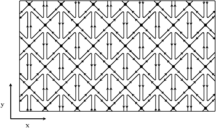
Figure 6.2: The figure, possibly related to the superconducting state in a cuprate, shows an array of strongly correlated center-vortex loops tiling the two-dimensional plane. If optimal screening of the electron charge located at the intersection point is provided by doping such that an attractive interaction between center-vortex loops due to Ampère’s Law becomes important, then the attractive force between equally directed center flux segments could lead to the indicated equilibrium configuration. For a given electron there are six neighbouring line segments two of which experience repulsion while the other four experience attraction. An overlap of flux lines would create new intersection points, each of mass $\propto m_{e}$ , which is topologically forbidden, thus leading to a repulsion at short distances.

Due to Ampère’s law equally directed electric flux lines attract each other, whereas oppositely directed flux lines experience a repulsive force. So, for a given center-vortex loop, there is an attractive interaction of four out of six line segments defined by the neighbouring electrons while the other two repulse each other. The existence of interactions between flux lines that are mediated by the photon is a consequence of the mixing between the gauge groups SU(2)_e and $\mathrm{SU(2)}_{\mbox{\tiny CMB}}$, the latter pertinent to the existence of propagating photons, see [10, 23]. It should be noticed that the spin projection of a given electron is equally directed for two of its neighbours while the other four have oppositely directed spins. This supports the observation that high $T_{c}$ superconductivity is an effect not related to $s$-wave pairing [52]. An overlap of flux lines would lead to additional intersection points which require an extra amount of energy $\Lambda_{C}$ for each intersection and is therefore energetically forbidden because the fluctuations in energy density of the system will not allow for the creation of an intersection of mass $m_{e}=511$ keV. This leads to a repulsive force as the spatial distance between adjacent vortex segments vanishes. In order that an equilibrium between attraction and repulsion where the intersection point is fixed with respect to its neighbours occurs, as it is depicted in Fig. 6.2, one needs a sufficiently low temperature (related to resolution) and an optimal screening of the Coulomb repulsion by the surrounding reservoir layers. If the temperature (resolution) falls below a critical value then the fluctuations of the intersection points relative to one another will vanish. Applying an external electric field parallel to the plane would set the stiff system of locked electrons in a collective motion with zero electric resistance. Macroscopically, this situation is illustrated by a stiff table cloth being pulled over the table in a frictionless way. The measured pseudo-gap phase in high $T_{c}$ superconductors will be addressed to local distortions in this highly ordered state. These distortions require an finite amount of energy and are due to insufficient screening and/or to much of a thermal noise.

Let us now turn to the recently discovered, new class of high $T_{c}$ superconductors that are based on oxypnictides (a class of materials including oxygen, an element of the nitrogen group (pnictogen), and one or more other elements). These do not seem to exhibit strong correlations between the electrons contained in the two-dimensional (FeAs) layers where the electron dynamics takes place, see [53]. If the behaviour of a two-dimensional system of non-interacting electrons, which are subjected to an environment represented by a parameter $\tau$, effectively is describable by a coarse-graining process in a statistical ensemble, as it is investigated in Chapter 5, then we should likely address the observation that the entropy vanishes at finite $\tau$ to this particular kind of high $T_{c}$ superconductivity. Namely, the observation that no variance of the ensemble average of the position of the electric charge is allowed for at a finite resolution is crucial for the statement that the two-dimensional system of free quasiparticles is void of any electric resistance. Free quasiparticles in the sense that explicit interactions between the electrons in the superconducting layer are absent, but the distortions induced by the noise of the environment is fully taken into account. Again, $\tau$ should be a monotonic function of temperature.

Chapter 7 Summary

In this thesis, we have investigated center-vortex loops with and without selfintersection, as they emerge in the confining phase of SU(2) Yang-Mills thermodynamics. In a noisy environment, center-vortex loops are subject to a spatial coarse-graining due to a motion by curvature that is described by a curve shortening flow. In a statistical description of ensembles of center-vortex loops which are (locally) embedded into a two-dimensional flat plane, we have defined an effective ‘action’ in purely geometric terms that is governed by a renormalization-group flow driven by the curve shrinking. The ‘action’ possesses a natural decomposition into a conformal and a non-conformal factor. ‘Observables’, such as the position of ‘center of mass’ ($N=0$), or the intersection point ($N=1$), are computed as ensemble averages of local or non-local operators on the curves.

We have made the observation that $N=0$ center-vortex loops exhibit a second-order transition to the conformal limit of vanishing curve length with a critical mean-field exponent of the coefficient: on average, center-vortex loops disappear from the spectrum of confining SU(2) Yang-Mills theory, thus generating an asymptotic mass gap. The evolution of the variance of the initially sharp position of ‘center of mass’ saturates at finite value within a finite decrease of resolution $Q$, the latter related to the resolving power used to probe to the system. These findings bear a strong family resemblance with the unitary time evolution of a free particle in quantum field theory.

Since we believe that $N=0$ center-vortex loops play the role of Majorana neutrinos [4], the concept of a neutrino rest mass is no longer applicable. Its mass is the result of the distortions induced by the environment it is embedded in and depends on the resolution. The disappearance of $N=0$ center-vortex loops from the excitation spectrum and the absence of a corresponding antiparticle would be manifestations of lepton-number violation forbidden in the Standard Model of Particle Physics.

In the case of one-fold intersecting center-vortex loops, we have obtained the unexpected result that a statistical ensemble of initial curves evolves into a highly ordered state. That is, only a particular member of the ensemble survives the process of two-dimensional spatial coarse-graining. As a consequence, the entropy attributed to the ensemble moves to a zero value for a sufficient decrease of resolution.

We have sketched an alternative approach to high-temperature superconductivity based on cuprates. The central observation that these depend highly on strong correlations between electrons trapped in a flat two-dimensional layer is attributed to an array of bow-tie-like simplices ($N=1$ center-vortex loops) tiling the plane. We have also speculated that the spontaneous emergence of order in an ensemble of planar $N=1$ center-vortex loops could be relevant for the recently discovered new class of oxypnictide layered high-temperature superconductors that do not seem to exhibit explicit, strong correlations between electrons within the superconducting (FeAs) planes.

In a sense, we have reversed the usage of the renormalization group. Instead of starting with a ‘physical’ action, from which an equation of motion follows, and demanding the system to be invariant under renormalization-group transformations, we have defined a geometric effective ‘action’ the coefficient of which is determined by a renormalization-group flow driven by a coarse-graining process (curve shrinking). Afterwards, physical ‘observables’, such as the center of mass or the localization of electric charge, were computed as mean values in a statistical ensemble. In a manner of speaking, we have ‘derived’ a statistically averaged ‘equation of motion’. In this context, we regard resolution over time (or temperature) as the more fundamental quantity describing a quantum mechanical or statistical system. However, this requires the introduction of a model that relates resolution to time (or temperature).

An obvious extension of our statistical approach would be the account of interactions between center-vortex loops; especially in view of two-dimensional systems exhibiting high-temperature superconductivity. At a first stage, this would include Coulomb interactions between the charges of $N=1$ center-vortex loops localized at the intersection point, and a delta-function-like repulsion due the topologically forbidden overlap of center-vortex loops (contact interaction). This could be done by adding interaction terms to the effective ‘action’ in the partition function that are weighted accordingly. Considering a multitude of configurations of initial curves of center-vortex loops, those configurations will be singled out the curves of which are most likely to survive the process of coarse-graining. However, the nontrivial issue arises how to gain a weight which relates the purely geometric ‘action’ to the one stemming from the electromagnetic interaction between center-vortex loops.

References

-
[1]
F. J. Hasert et al., Search for
elastic muon-neutrino electron scattering, Phys. Lett. B 46,
121 (1973).
F. J. Hasert et al., Observation of neutrino-like interactions without muon or electron in the Gargamelle neutrino experiment, Phys. Lett. B 46, 138 (1973). - [2] A. Jaffe and E. Witten, Quantum Yang-Mills Theory, Clay Mathematics Institute Millenium Prize problem, http://www.claymath.org/millennium/Yang-Mills_Theory (2000).
- [3] C. Amsler et al. [Particle Data Group], Review of Particle Physics, Phys. Lett. B 667, 1 (2008).
-
[4]
H. V. Klapdor-Kleingrothaus, I. V. Krivosheina, A. Dietz,
and O. Chkvorets, Search for neutrinoless decay with
enriched 76Ge in Gran Sasso 1990-2003,
Phys. Lett. B 586, 198 (2004).
H. V. Klapdor-Kleingrothaus, From nuclear physics to physics beyond the Standard Model: First evidence for lepton number violation and the Majorana character of neutrinos, Int. J. Mod. Phys. D 13, 2107 (2004).
H. V. Klapdor-Kleingrothaus and I. V. Krivosheina, The evidence for the observation of decay: The identification of events from the full spectra, Mod. Phys. Lett. A 21, 1547 (2006). - [5] V. M. Lobashev et al., Direct search for mass of neutrino and anomaly in the tritium beta-spectrum, Phys. Lett. B 460, 227 (1999).
- [6] Ch. Kraus et al., Final results from phase II of the Mainz neutrino mass searching tritium decay, Eur. Phys. C 40, 447 (2005).
- [7] A. D. Linde, Infrared problem in thermodynamics of the Yang-Mills gas, Phys. Lett. B 96, 289 (1980).
- [8] L. H. Ryder, Quantum Field Theory, Cambridge University Press (1996).
- [9] J. G. Bednorz and K. A. Müller, Possible high superconductivity in the Ba-La-Cu-O system, Z. Phys. B 64, 189 (1986).
-
[10]
R. Hofmann, Nonperturbative approach to
Yang-Mills thermodynamics, Int. J. Mod. Phys. A 20, 4123
(2005);
Erratum-ibid. A 21, 6515 (2006).
R. Hofmann, Yang-Mills thermodynamics, arXiv:hep-th/0710.0962 (2007). - [11] H. B. Nielsen and P. Olesen, Vortex-line models for dual strings, Nucl. Phys. B 61, 45 (1973).
- [12] G. ’t Hooft, On the phase transition towards permanent quark confinement, Nucl. Phys. B 138, 1 (1978).
- [13] L. Faddeev and A. J. Niemi, Stable knot-like structures in classical field theory, Nature 387, 58 (1997).
- [14] W. T. Kelvin and P. G. Tait, Treatise on Natural Philosophy, 2 vols., Cambridge University Press (1867).
- [15] http://www.sandia.gov/news-center/news-releases/2006/physics-astron/hottest-z-output.html (2006).
- [16] F. Giacosa, R. Hofmann, and M. Schwarz, Explosive Pinch, Mod. Phys. Lett. A 21, 2709 (2006).
-
[17]
L. Faddeev and A. J. Niemi, Partially dual
variables in SU(2) Yang-Mills theory, Phys. Rev. Lett. 82, 1624 (1999).
L. Faddeev and A. J. Niemi, Aspects of electric and magnetic variables in SU(2) Yang-Mills theory, Phys. Lett. B 525, 195 (2002).
L. Faddeev and A. J. Niemi, Spin-charge separation, conformal covariance and the SU(2) Yang-Mills theory, Nucl. Phys. B 776, 38 (2007). - [18] R. P. Feynman, The Principle of Least Action in Quantum Mechanics, Princeton University Ph. D. thesis, University Microfilms Publication No. 2984, Ann Arbor (1942).
- [19] A. A. Belavin, A. M. Polyakov, A. S. Schwartz, and Yu. S. Tyupkin, Pseudoparticle solutions of the Yang-Mills equations, Phys. Lett. B 59, 85 (1975).
- [20] D. Diakonov, N. Gromov, V. Petrov, and S. Slizovskiy, Quantum weights of dyons and of instantons with nontrivial holonomy, Phys. Rev. D 70, 036003 (2004).
- [21] F. Giacosa and R. Hofmann, Thermal ground state in deconfining Yang-Mills thermodynamics, PTP 118, 759 (2007).
- [22] U. Herbst and R. Hofmann, Asymptotic freedom and compositeness, arXiv:hep-th/0411214 (2004).
- [23] F. Giacosa and R. Hofmann, A Planck-scale axion and SU(2) Yang-Mills dynamics: Present acceleration and the fate of the photon, Eur. Phys. J. C 50, 635 (2007).
- [24] S. Scheffler, R. Hofmann, and I.-O. Stamatestu, Scalar field theory with a non-standard potential, Phys. Rev. D 77, 065015 (2008).
- [25] R. Hofmann, Yang-Mills thermodynamics at low temperature, Mod. Phys. Lett. A 22, 2657 (2007).
- [26] R. Hofmann, Yang-Mills thermodynamics: The confining phase, arXiv:hep-th/0508212 (2005).
- [27] E. R. Williams, J. E. Faller, and H. A. Hill, New experimental test of Coulomb’s law: A laboratory upper limit on the photon rest mass, Phys. Rev. Lett. 26, 721 (1971).
- [28] R. Hofmann, A strongly interacting SU(2) pure gauge theory and the nature of light, Talk given at 29th Johns Hopkins workshop in Theoretical Physics: Strong Matter in the Heavens, Budapest, Hungary, 1-3 Aug 2005. Published in PoS JHW2005, 021 (2006).
- [29] M. Schwarz, R. Hofmann, and F. Giacosa, Radiative corrections to the pressure and the one-loop polarization tensor of massless modes in SU(2) Yang-Mills thermodynamics, Int. J. Mod. Phys. A 22, 1213 (2007).
- [30] M. Schwarz, R. Hofmann, F. Giacosa, Gap in the black-body spectrum at low temperatures, JHEP 0702, 091 (2007).
- [31] L. B. G. Knee and C. M. Brunt, A massive cloud of cold atomic hydrogen in the outer Galaxy, Nature 412, 308 (2008).
- [32] W. P. Thurston, The Geometry and Topology of Three-Manifolds, Lecture notes (1980), http://www.msri.org/publications/books/gt3m/ (2002).
- [33] B. Leep, Geometrisierung 3-dimensionaler Mannigfaltigkeiten und Ricci-Fluß, DMV-Mitteilungen 14, 213 (2006).
- [34] P. W. Topping, Lectures on the Ricci flow, L.M.S. Lecture note series 325 C.U.P., http://www.warwick.ac.uk/m̃aseq/RFnotes.html (2006).
- [35] W. P. Thurston, Three dimensional manifolds, Kleinian groups and hyperbolic geometry, Bull. Amer. Math. Soc. (N.S.) 6, no. 3, 357 (1982).
- [36] R. S. Hamilton, Three-manifolds with positive Ricci curvature, J. Differential Geometry 17, 255 (1982).
-
[37]
G. Perelman, The entropy formula for the Ricci
flow
and its geometric applications, arXiv:math/0211159.
G. Perelman, Ricci flow with surgery on three-manifolds, arXiv:math/0303109.
G. Perelman, Finite extinction time for the solutions to the Ricci flow on certain three-manifolds, arXiv:math/0307245. - [38] M. Gage and R. S. Hamilton, The heat equation shrinking convex plane curves, J. Differential Geometry 23, 69 (1986).
- [39] M. A. Grayson, The heat-equation shrinks embedded plane curves to round points, J. Differential Geometry 26, 285 (1987).
- [40] M. A. Grayson, The shape of a figure-eight under the curve shortening flow, Invent. Math. 96, 177 (1989).
- [41] M. A. Grayson, Shortening embedded curves, Annals of Mathematics 129, 71 (1989).
-
[42]
S. L. Smith, M. E. Broucke, and B. A. Francis,
Curve shortening and its application to multi-agent systems, in
proc. 44th IEEE Conference on Decision and Control, and European
Control
Conference 2005, Seville, Spain, Dec. 12-15 (2005).
S. L. Smith, M. E. Broucke, and B. A. Francis, Curve shortening and the rendezvous problem for mobile autonomous robots, arXiv:cs/0605070 (2006). - [43] M. Gage, An isoperimetric inequality with applications to curve shortening, Duke Mathematical Journal, 50(3), 1225 (1983).
- [44] M. Gage, Curve shortening makes convex curves circular, Invent. Math. 76, 357 (1984).
- [45] K.-S. Chou and X.-P. Zhu, The Curve Shortening Problem, Chapman and Hall (2001).
- [46] S. J. Altschuler, Singularities of the curve shrinking flow for space curves, J. Differential Geometry. 34, 491 (1991).
- [47] S. J. Altschuler and M. A. Grayson, Shortening space curves and flow through singularities, J. Differential Geometry. 35, 283 (1992).
- [48] M. A. Grayson, Shortening embedded curves, Annals of Mathematics, 129, 71 (1989).
- [49] F. Cao, Geometric Curve Evolution and Image Processing, Springer (2003).
- [50] M. G. Haines, P. D. LePell, C. A. Coverdale, B. Jones, C. Deeney, and J. P. Apruzese, Ion viscous heating in a magnetohydrodynamically unstable Pinch at over Kelvin, Phys. Rev. Lett. 96, 075003 (2006).
-
[51]
P. W. Anderson, Present status of the theory of
high cuprates, arXiv:cond-mat/0510053 (2005).
P. W. Anderson, Twenty years of talking past each other: The theory of high , Physica C 460-462, 3 (2007). - [52] A. Garg, M. Randeria, and N. Trivedi, Strong correlations make high-temperature superconductors robust against disorder, Nature Physics Advance online publication 10.1038/nphys1026 (2008).
- [53] H.-H. Klauss and B. Büchner, Neuer Goldrausch in der Supraleitung?, Physik Journal 7, 18 (2008).