Neutrino oscillograms of the Earth and CP violation in neutrino oscillations

Abstract

An analysis of 3-flavour neutrinos oscillations inside the Earth is presented in terms of the oscillograms – contour plots of oscillation probabilities in the plane neutrino energy – nadir angle. Special attention is paid to CP violation in neutrino oscillations in the Earth.

1 INTRODUCTION

Neutrino oscillograms of the Earth are contours of constant oscillation or survival probabilities in the plane of neutrino energy and nadir or zenith angle of neutrino trajectory. They encode information on both the neutrino parameters and the Earth density profile and proved to be a very useful and illuminating tool for analyzing neutrino oscillations in the Earth.

The oscillograms exhibit a very rich structure with local and global maxima and minima (including the MSW resonance maxima in the mantle and core of the Earth), saddle points and the parametric enhancement ridges (Fig. 1). It was shown in [1] that all these features can be readily understood in terms of various realizations of just two conditions: the generalized amplitude (collinearity) and phase conditions. The study in [1] was performed in the limit $\Delta m_{21}^{2}=0$; in the present talk, based on [2], the results for $\Delta m_{21}^{2}\neq 0$ are presented.

2 OSCILLOGRAMS FOR 3-FLAVOUR NEUTRINO OSCILLATIONS

In the full 3-flavour framework with $\Delta m_{21}^{2}\neq 0$ and $\theta_{13}\neq 0$, the oscillograms have non-trivial structure both at low and high energies. Oscillations at low energies are dominated by the solar channel, whereas those at higher energies are mainly driven by the atmospheric parameters $(\Delta m_{31}^{2},\theta_{13})$ (see Fig.1).

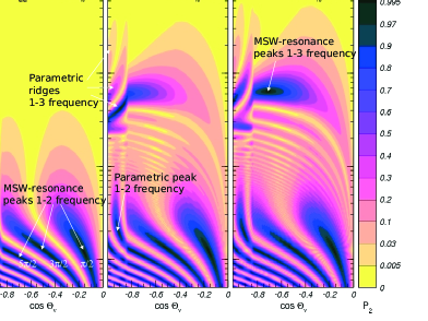
Figure 1: Oscillograms for $1-P_{ee}$ for three different values of $\theta_{13}$.

The main qualitatively new feature of 3-flavour oscillations as compared to 2-flavour ones is the possibility of CP violation. Its effect can be conveniently studied in terms of CP-oscillograms, which are defined as contour plots of equal probability difference

$$\Delta P_{\mu e}^{\rm CP}\equiv P_{\mu e}(\delta)-P_{\mu e}(\delta_{\rm th})\,,$$ (1)

where $\delta$ is the true value of the CP violating phase and $\delta_{\rm th}$ is the assumed, or theoretical, value which we want to test. The CP-oscillograms have a rather complex domain-like structure (see Fig. 2); however, this structure can be readily understood and interpreted in terms of three grids of curves, as we discuss next.

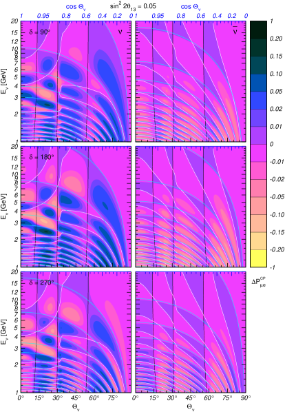
Figure 2: Oscillograms for the difference of probabilities $\Delta P_{\mu e}^{\rm CP}=P_{\mu e}(\delta)-P_{\mu e}(\delta_{\rm th})$ with $\delta_{\rm th}=0^{\circ}$. Shown are the solar (black), atmospheric (white) and interference phase condition (cyan) curves.

The oscillation probability $P_{\mu e}$ can be conveniently written as

$$P_{\mu e}=|c_{23}\,A_{e2}\,e^{i\delta}+s_{23}\,A_{e3}|^{2}\,,$$ (2)

where the amplitudes $A_{e2}$ and $A_{e3}$ are independent of $\theta_{23}$ and CP-violating phase $\delta$. To leading order in small parameters $s_{13}$ and $\Delta m_{21}^{2}/\Delta m_{31}^{2}$, $A_{e2}$ depends only on the solar oscillation parameters and $A_{e3}$, only on the atmospheric ones:

$$A_{e2}\simeq A_{S}(\theta_{12},\,\Delta m_{21}^{2})\,,~{}~{}~{}A_{e3}\simeq A_{A}(\theta_{13},\,\Delta m_{31}^{2})\,,$$ (3)

i.e., these amplitudes approximately coincide with, respectively, the solar and atmospheric contributions to the amplitude of $\nu_{\mu}\leftrightarrow\nu_{e}$ oscillations. From eq. (2) we find

$$P_{\mu e}\!\!\!\! = \!\!\!\!c_{23}^{2}|A_{S}|^{2}+s_{23}^{2}|A_{A}|^{2}~{}~{}~{}~{}~{}$$ (4)

$$\!\!\!\!+2s_{23}c_{23}|A_{S}||A_{A}|\cos(\phi+\delta)\,,$$

where $\phi=arg(A_{S}A_{A}^{*})$. Only the last term in (4) depends on $\delta$; the condition of vanishing $\Delta P_{\mu e}$ (i.e. $P_{\mu e}(\delta)=P_{\mu e}(\delta_{\rm th})$) therefore corresponds to

$$|A_{S}||A_{A}|\cos(\phi+\delta)=|A_{S}||A_{A}|\cos(\phi+\delta_{th})\,.$$ (5)

There are three non-trivial realisations of this condition:

• $A_{S}~{}=~{}0$  ($\Rightarrow$ solar “magic” lines)

• $A_{A}~{}=~{}0$  ($\Rightarrow$ atm. “magic” curves)

• $(\phi+\delta_{th})=-(\phi+\delta)+2\pi l$,   or  
  $\phi=-(\delta+\delta_{th})/2+\pi k.$

There is also, of course, the trivial realization, $\delta_{\rm th}=\delta+2\pi n$, when the true and assumed values of  $\delta$ coincide. The above three conditions give rise to three grids of curves, which delineate the different domains in the CP oscillograms (Fig. 2); they have a very simple physical interpretation. We shall now discuss these conditions in the energy region between the 1-2 and 1-3 MSW resonances; the results for other energy domains can be found in [2].

2.1 Solar “magic” curves

The condition of vanishing solar channel contribution to the oscillation probability, $A_{S}=0$, in the constant matter density approximation can be written as $\sin^{2}(\omega_{12}L)=0$ (i.e. $\omega_{12}L=\pi n$), where $\omega_{12}$ is the solar oscillation frequency. At energies exceeding the 1-2 resonance energies in the mantle and in the core of the Earth, $E\gtrsim 0.5$ GeV, one has $\omega_{12}\simeq V/2$, where $V=\sqrt{2}G_{F}N_{e}$ is the matter-induced potential of neutrinos. The condition $A_{S}=0$ therefore takes the form

$$L(\Theta_{\nu})\simeq\frac{2\pi n}{V}\,,$$ (6)

where $L(\Theta_{\nu})$ is the nadir angle dependent length of the neutrino trajectory in the Earth. Note that the condition (6) is energy independent and determines the baselines for which the “solar” contribution to the probability vanishes. In the plane $(\Theta_{\nu},E_{\nu})$ it represents nearly vertical lines $\Theta_{\nu}\approx\text{const}$ (black lines in Fig. 2).

There are three solar magic lines which correspond to $n=1$ (in the mantle domain) and $n=2,3$ (in the core domain). The existence of a baseline ($L\approx 7600$ km) for which the probability of $\nu_{e}\leftrightarrow\nu_{\mu}$ oscillations in the Earth is approximately independent of the “solar” parameters ($\Delta m_{21}^{2}$, $\theta_{12}$) and of the CP-phase $\delta$ was first pointed out in [3] and later discussed in a number of publications (see [4, 5] and references therein). This baseline was dubbed “magic” in [4]. The interpretation of this baseline as corresponding to vanishing “solar” amplitude $A_{e2}$, according to eq. (6) with $n=1$, was given in [5]. It was also shown there that for neutrino trajectories crossing the core of the Earth there exist two more solar “magic” baselines, corresponding to the oscillation phase equal $\pi n$ with $n=2$ and 3, and the existence of the atmospheric “magic” curves was pointed out.

2.2 Atmospheric “magic curves”

The second realization of the condition (5) corresponds to vanishing atmospheric amplitude, $A_{A}=0$. In this case, like on the solar “magic” lines, the probabilities of $\nu_{e}\leftrightarrow\nu_{\mu}$ (as well as $\nu_{e}\leftrightarrow\nu_{\tau}$) oscillations are independent of the CP-violating phase. In addition, they do not depend on the atmospheric parameters $\Delta m_{31}^{2}$ and $\theta_{13}$.

The properties of atmospheric “magic” curves can be easily understood in the constant density approximation, in which the condition $A_{A}=0$ is satisfied when $\sin^{2}(\omega_{31}L(\Theta_{\nu}))=0$, i.e. $\omega_{31}L(\Theta_{\nu})=\pi k$, $k=1,2,\dots$. For energies which are not too close to the atmospheric MSW resonance energy, this condition reduces to

$$E\simeq\frac{\Delta m_{31}^{2}L(\Theta_{\nu})}{|4\pi k\pm 2VL(\Theta_{\nu})|}\,,$$ (7)

which corresponds to the bent curves in the $(\Theta_{\nu},E_{\nu})$ plane (shown in white in Fig. 2).

2.3 The interference phase condition

The third of the above mentioned realizations of the condition (6) depends on the interference phase between the amplitudes $A_{S}$ and $A_{A}$ and therefore we shall call it the interference phase condition. In the energy region between the 1-2 and 1-3 resonances we have $\phi\approx\Delta m_{31}^{2}L/4E$, i.e. in the first approximation $\phi$ does not depend on the matter density. The interference phase condition then takes the form $\Delta m_{31}^{2}L/4E=-(\delta+\delta_{\rm th})/2+\pi l$, or

$$E_{\nu}=\frac{\Delta m_{31}^{2}L(\Theta_{\nu})}{4\pi l-2(\delta+\delta_{\rm th})}\,.$$ (8)

From the comparison of eqs. (8) and (7) it follows that the interference phase curves (shown in cyan in the oscillogram of Fig. 2) are similar to atmospheric curves, but are steeper than the latter for $\nu$’s and less steep for $\bar{\nu}$’s.

3 CONCLUSIONS

It can be seen from Fig. 2 that the three grids of curves discussed above – the solar and atmospheric “magic” ones and the interference phase curves – give a very accurate description of the borders between the domains. On these borders the probability difference $\Delta P_{\mu e}^{\rm CP}=P_{\mu e}(\delta)-P_{\mu e}(\delta_{\rm th})$ vanishes, and therefore there is no sensitivity to the phase $\delta$. The regions of maximal sensitivity to the CP-violating phase correspond to the central parts of the domains.

Our analysis has been performed in terms of the oscillation probabilities; a more realistic study which considers the number of events in future detectors is currently under way.

References

- [1] E.Kh. Akhmedov, M. Maltoni and A.Yu. Smirnov, JHEP 0705 (2007) 077 [arXiv:hep-ph/0612285].
- [2] E.Kh. Akhmedov, M. Maltoni and A.Yu. Smirnov, JHEP 0806 (2008) 072 [arXiv:0804.1466 [hep-ph]].
- [3] V. Barger, D. Marfatia, and K. Whisnant, Phys. Rev. D65 (2002) 073023, [hep-ph/0112119].
- [4] P. Huber, J. Phys. G29 (2003) 1853, [hep-ph/0210140].
- [5] A.Yu. Smirnov, hep-ph/0610198.