Rare decays $B_{s}\to l^{+}l^{-}$ and $B\to Kl^{+}l^{-}$ in
the topcolor-assisted technicolor model

Abstract

We examine the rare decays $B_{s}\to l^{+}l^{-}$ and $B\to Kl^{+}l^{-}$ in the framework of the topcolor-assisted technicolor ($TC2$) model. The contributions of the new particles predicted by this model to these rare decay processes are evaluated. We find that the values of their branching ratios are larger than the standard model predictions by one order of magnitude in wide range of the parameter space. The longitudinal polarization asymmetry of leptons in $B_{s}\to l^{+}l^{-}$ can approach ${\cal O}(10^{-2})$. The forward-backward asymmetry of leptons in $B\to Kl^{+}l^{-}$ is not large enough to be measured in future experiments. We also give some discussions about the branching ratios and the asymmetry observables related to these rare decay processes in the littlest Higgs model with T-parity.

I. Introduction

The study of pure leptonic and semileptonic decays of B meson is one of the most important tasks of B physics both theoretically and experimentally. These rare B decays are sensitive to new physics ($NP$) and their signals are useful for testing the standard model ($SM$) [1]. So far, a lot of works have been concentrated on these decays. In the $SM$, there are no flavor changing neutral current ($FCNC$) processes at the tree level and the leading contributions to these decays come from the one-loop level. So these rare decays are rather sensitive to the contributions from the $NP$ models beyond the $SM$. Studying of the observables of the asymmetries, such as the $CP$ asymmetry [2], longitudinal polarization ($LP$) asymmetry $A_{LP}$ [3], and forward-backward ($FB$) asymmetry $A_{FB}$ [4] etc, interests experiments in testing $NP$. Certainly, their detection requires excellent triggering and identification of leptons with low misidentification rates for hadrons. The precision measurement needs further studying.

The quark level transition $b\to sl^{+}l^{-}$ is responsible for both the purely leptonic decays $B_{s}\to l^{+}l^{-}$ and the semileptonic decays $B\to Kl^{+}l^{-}$($l=e,\mu,\tau$). The decay $B_{s}\to\mu^{+}\mu^{-}$ will be one of the most important rare B decays to be studied at the upcoming large hadron collider ($LHC$), and so far the upper bound on its branching ratio is [5]

$$Br(B_{s}\to\mu^{+}\mu^{-})<5.8\times 10^{-8}(95\%~{}{\rm C.L.}).$$ (1)

The branching ratios of $B\to Kl^{+}l^{-}$ observed by BaBar collaboration and Belle collaboration are [6, 7]

$$Br(B\rightarrow Kl^{+}l^{-})=(5.7^{+2.2}_{-1.8})\times 10^{-7},$$ (2)

which is close to the $SM$ prediction [1, 8]. However, due to the errors in the determination of the hadronic form factors and the Cabibbo-Kobayashi-Maskawa ($CKM$) matrix element $|V_{ts}|$, there is about $20\%$ uncertainty in $SM$ prediction. The experimental measurement values of rare decay processes $B_{s}\to e^{+}e^{-},\tau^{+}\tau^{-}$ will be discussed later.

We also consider other observables of the purely leptonic and semileptonic decays for the $B$ meson, which are sensitive to scalar/pesudoscalar new physics ($SPNP$) contributions to $b\to s$ transitions. They are forward-backward asymmetry $A_{FB}$ of leptons in $B\to Kl^{+}l^{-}$ and longitudinal polarization asymmetry $A_{LP}$ of leptons in $B_{s}\to l^{+}l^{-}$. The observable $A_{LP}$ was introduced in Reference [3], though the corresponding analysis in the context of $K\to\mu^{+}\mu^{-}$ had been carried out earlier [9]. The average $A_{FB}$ in the rare decay processes $B\to Kl^{+}l^{-}$ has been measured by BaBar collaboration as [6]

$$\left\langle A_{FB}\right\rangle=0.15_{-0.23}^{+0.21}\pm 0.08.$$ (3)

This measured value is close to zero and has a high experimental error. As the values of $A_{LP}$ and $A_{FB}$ predicted in the $SM$ are nearly zero, any nonzero value of one of these asymmetries is a signal for $NP$. This is the main reason we focus on these observables.

In literature, there are numerous studies of the quark level decays $b\to sl^{+}l^{-}$ both in the $SM$ and in some $NP$ models. Recently, Reference [10, 11] have studied the sensitivity of these rare decay processes to the radius $R$ in the universal extra dimension ($UED$) model. In the supersymmetry ($SUSY$) models, extensive works have been taken to the branching ratios of these rare decays, and some of these discussions are related to the asymmetry aspect [12, 13]. These decays have also been discussed in the littlest Higgs model with T-parity (called the $LHT$ model) [14], they have verified that the $LHT$ model can enhance the branching ratios of these decays [15]. However, they have not discussed the asymmetry observables, we will give some discussions on these observables in the framework of the $LHT$ model.

In the framework of the topcolor-assisted technicolor ($TC2$) model [16], Reference [17] has calculated the branching ratios of quark level $b\to sl^{+}l^{-}$ decays. They consider the contributions of the non-universal gauge boson $Z^{\prime}$ predicted by this model. Their numerical results show that the enhancement is quite large when the mass of $Z^{\prime}$ is small. Reference [18] has calculated the contributions coming from the pseudoscalar top-pions predicted by this model to the branching ratios of the decays $B_{s}\to l^{+}l^{-}$. Reference [19] has evaluated the contributions from both the neutral and charged scalars predicted by this model, the branching ratios can be enhanced over the $SM$ predictions by two orders of magnitude in some part of parameter space. So far, we have not seen the study of the asymmetry observables for these two decays in the framework of the $TC2$ model, and furthermore the former discussions on the branching ratios have not considered the contributions induced by all the particles predicted by this model.

In this paper, we consider the contributions coming from all of the new particles predicted by the $TC2$ model to the branching ratios and asymmetries related to the rare decay processes $b\to sl^{+}l^{-}$. Compared with the predictions in the $SM$, our results show that the contributions to the branching ratios and the asymmetries come from two aspects. First, the Wilson coefficients of these processes receive additional contributions from the non-universal gauge boson $Z^{\prime}$ and charged top-pions. Second, the neutral top-pion and top-Higgs can give contributions through newly introduced scalar/pesudoscalar operators. For comparison, we also give our results in the $LHT$ model, considering different parametrization scenarios.

This paper is arranged as follows. In the following section, we will summarize some elementary features of the $TC2$ model. In Sec. III we present our calculation on the decay processes $B_{s}\to l^{+}l^{-}$. The decay processes $B\to Kl^{+}l^{-}$ will be studied in the Sec. IV. In Sec. V we give simple discussions on the above questions in the $LHT$ model. Conclusions are given in Sec. VI.

II. The $\rm{TC2}$ model

The $TC2$ model [16] is one kind of the phenomenological viable models, which has all essential features of the topcolor scenario. The $TC2$ model generates the large quark mass through the formation of a dynamical $t\bar{t}$ condensation and provides possible dynamical mechanism for electroweak symmetry breaking ($EWSB$). The physical top-pions($\pi_{t}^{0,\pm}$), the non-universal gauge boson ($Z^{\prime}$) and the top-Higgs ($h_{t}^{0}$) are predicted. The presence of the physical top-pions $\pi_{t}^{0,\pm}$ in the low energy spectrum is an inevitable feature of the topcolor scenario, regardless of the dynamics responsible for $EWSB$ and other quark mass. The flavor-diagonal ($FD$) couplings of top-pions to fermions can be written as [16, 20]:

$$\frac{m_{t}^{*}}{\sqrt{2}F_{\pi}}\frac{\sqrt{\nu_{w}^{2}-F_{\pi}^{2}}}{\nu_{w}}\left[i\bar{t}\gamma^{5}t\pi_{t}^{0}+\sqrt{2}\bar{t}_{R}b_{L}\pi_{t}^{+}+\sqrt{2}\bar{b}_{L}t_{R}\pi_{t}^{-}\right]$$

$$+\frac{m_{b}^{*}}{\sqrt{2}F_{\pi}}\left[i\bar{b}\gamma^{5}b\pi_{t}^{0}+\sqrt{2}\bar{t}_{L}b_{R}\pi_{t}^{+}+\sqrt{2}\bar{b}_{R}t_{L}\pi_{t}^{-}\right]+\frac{m_{l}}{\nu}\bar{l}\gamma^{5}l\pi^{0}_{t},$$ (4)

where $m_{t}^{*}=m_{t}(1-\varepsilon)$, $\nu_{w}=\nu/\sqrt{2}=174\rm~{}GeV$, $F_{\pi}\approx 50\rm~{}GeV$ is the top-pion decay constant. The ETC interactions give rise to the masses of the ordinary fermions including a very small portion of the top quark mass, namely $\varepsilon m_{t}$ with a model dependent parameter $\varepsilon\ll 1$, and $m_{b}^{*}=m_{b}-0.1\varepsilon m_{t}$ [25]. The factor $\frac{\sqrt{\nu_{w}^{2}-F_{\pi}^{2}}}{\nu_{w}}$ reflects mixing effect between top-pions and the Goldstone bosons.

For the $TC2$ model, the underlying interactions, topcolor interactions, are non-universal and therefore do not posses Glashow-Iliopoulos-Maiani ($GIM$) mechanism [26]. One of the most interesting features of $\pi_{t}^{0,\pm}$ is that they have large Yukawa couplings to the third-generation quarks and can induce the tree-level flavor changing ($FC$) couplings [27, 28]. When one writes the non-universal interactions in the quark mass eigen-basis, it can induce the tree-level $FC$ couplings. The $FC$ couplings of top-pions to quarks can be written as [17, 27]:

$$\frac{m_{t}^{*}}{\sqrt{2}F_{\pi}}\frac{\sqrt{\nu_{w}^{2}-F_{\pi}^{2}}}{\nu_{w}}\left[iK_{UR}^{tc}K_{UL}^{tt^{*}}\bar{t}_{L}c_{R}\pi_{t}^{0}+\sqrt{2}K_{UR}^{tc^{*}}K_{DL}^{bb}\bar{c}_{R}b_{L}\pi_{t}^{+}+\sqrt{2}K_{UR}^{tc}K_{DL}^{bb^{*}}\bar{b}_{L}c_{R}\pi_{t}^{-}\right.$$

$$\hskip 42.67912pt\left.+\sqrt{2}K_{UR}^{tc^{*}}K_{DL}^{ss}\bar{t}_{R}s_{L}\pi_{t}^{+}+\sqrt{2}K_{UR}^{tc}K_{DL}^{ss^{*}}\bar{s}_{L}t_{R}\pi_{t}^{-}\right],$$ (5)

where $K_{UL(R)}$ and $K_{DL(R)}$ are rotation matrices that diagonalize the up-quark and down-quark mass matrices $M_{U}$ and $M_{D}$, i.e., $K_{UL}^{+}M_{U}K_{UR}=M_{U}^{dia}$ and $K_{DL}^{+}M_{D}K_{DR}=M_{D}^{dia}$, for which the $CKM$ matrix is defined as $V=K_{UL}^{+}K_{DL}$. To yield a realistic form of the $CKM$ matrix $V$, it has been shown that the values of the coupling parameters can be taken as [27]:

$$K_{UL}^{tt}\approx K_{DL}^{bb}\approx K_{DL}^{ss}\approx 1,\hskip 28.45274ptK_{UR}^{tc}\leq\sqrt{2\varepsilon-\varepsilon^{2}}.$$ (6)

In the following calculation, we will take $K_{UR}^{tc}=\sqrt{2\varepsilon-\varepsilon^{2}}$ and take $\varepsilon$ as in the range of $0.03-0.1$ [16]. The $TC2$ model predicts the existence of the top-Higgs $h_{t}^{0}$, which is a $t\bar{t}$ bound and analogous to the $\sigma$ particle in low energy $QCD$. It has similar Feynman rules as the $SM$ Higgs boson, so we don’t list them.

Another significant feature of the $TC2$ model is the existence of non-universal gauge boson $Z^{\prime}$, which may provide significant contributions to some $FCNC$ processes because of its $FC$ couplings to fermions. The $FC$ $b-s$ coupling to $Z^{\prime}$ can be written as [29]:

$${\cal L}^{FC}_{Z^{\prime}}=-\frac{g_{1}}{2}\cot{\theta^{\prime}}Z^{\prime\mu}\left\{\frac{1}{3}D_{L}^{bb}D_{L}^{bs*}\bar{s}_{L}\gamma_{\mu}b_{L}-\frac{2}{3}D_{R}^{bb}D_{R}^{bs*}\bar{s}_{R}\gamma_{\mu}b_{R}+{\rm h.c.}\right\},$$ (7)

$D_{L},D_{R}$ are matrices which rotate the down-type left and right hand quarks from the quark field to mass eigen-basis. The $FD$ couplings of $Z^{\prime}$ to fermions, which are relative to our calculation, can be written as [16, 17, 20, 30]:

$${\cal L}^{FD}_{Z^{\prime}} = -\sqrt{4\pi K_{1}}\left\{Z^{\prime}_{\mu}\left[\frac{1}{2}\bar{\tau}_{L}\gamma^{\mu}\tau_{L}-\bar{\tau}_{R}\gamma^{\mu}\tau_{R}+\frac{1}{6}\bar{t}_{L}\gamma^{\mu}t_{L}+\frac{1}{6}\bar{b}_{L}\gamma^{\mu}b_{L}+\frac{2}{3}\bar{t}_{R}\gamma^{\mu}t_{R}\right.\right.$$ (8)

$$- \left.\left.\frac{1}{3}\bar{b}_{R}\gamma^{\mu}b_{R}\right]-\tan^{2}\theta^{\prime}Z^{\prime}_{\mu}\left[\frac{1}{6}\bar{s}_{L}\gamma^{\mu}s_{L}-\frac{1}{3}\bar{s}_{R}\gamma^{\mu}s_{R}-\frac{1}{2}\bar{\mu}_{L}\gamma^{\mu}\mu_{L}-\bar{\mu}_{R}\gamma^{\mu}\mu_{R}\right.\right.$$

$$- \left.\left.\frac{1}{2}\bar{e}_{L}\gamma^{\mu}e_{L}-\bar{e}_{R}\gamma^{\mu}e_{R}\right]\right\},$$

where $K_{1}$ is the coupling constant and $\theta^{\prime}$ is the mixing angle with $\tan\theta^{\prime}=\frac{g_{1}}{\sqrt{4\pi K_{1}}}$. $g_{1}$ is the ordinary hypercharge gauge coupling constant.

In the following sections, we will use the above formulae to calculate the contributions of the $TC2$ model to the rare decay processes $B_{s}\to l^{+}l^{-}$ and $B\to Kl^{+}l^{-}$.

III. The contributions of the $\rm{TC2}$ model to the rare decay processes      $B_{s}\to l^{+}l^{-}$

The $TC2$ model can give contributions to rare B decays two different ways, either through the new contributions to the Wilson coefficients or through the new scalar or pseudoscalar operators. The most general model independent form of the effective Hamilton for the decays $B_{s}\to l^{+}l^{-}$ including the contributions of $NP$ has the form:

$$H(B_{s}\to l^{+}l^{-})=H_{0}+H_{1}\,$$ (9)

with

$$H_{0} = \frac{\alpha G_{F}}{2\sqrt{2}\pi}\left(V_{ts}^{*}V_{tb}\right)\,\biggl{\{}R_{A}(\bar{s}\,\gamma_{\mu}\gamma_{5}\,b)(\bar{l}\,\gamma^{\mu}\gamma_{5}\,l)\biggr{\}}\;,$$ (10)

$$H_{1}=\frac{\alpha G_{F}}{\sqrt{2}\pi}(V_{tb}V^{*}_{ts})\biggl{\{}R_{S}\,(\bar{s}\,P_{R}\,b)\,(\bar{l}\,l)+R_{P}\,(\bar{s}\,P_{R}\,b)\,(\bar{l}\gamma_{5}l)\biggr{\}}\;.$$ (11)

Where $H_{0}$ represents the $SM$ operators and $H_{1}$ represents the $SPNP$ operators. Here $P_{L,R}=(1\mp\gamma_{5})/2$, $R_{S}$, $R_{P}$ and $R_{A}$ denote the strengths of the scalar, pseudoscalar, and axial vector operators, respectively [31]. In our analysis we assume that there are no additional $CP$ phases apart from the single $CKM$ phase, thus $R_{S}$ and $R_{P}$ are real. In the $SM$, the scalar and pseudoscalar couplings $R_{S}$ and $R_{P}$ receive contributions from the penguin diagrams with physical and unphysical neutral scalar exchange and are highly suppressed to ${\cal O}(10^{-5})$. The coupling constant of the axial vector operator $R_{A}$ can be expressed as $R_{A}={Y^{SM}(x)}/{\sin^{2}\theta_{w}}$, where $Y^{SM}(x)$ is the $SM$ Inami-Lim function [32], which has been listed in Appendix A. These coupling constants will receive contributions coming from the non-universal gauge boson $Z^{\prime}$ and the scalars $\pi_{t}^{0,\pm},h^{0}_{t}$.

A. The contributions of the nonuniversal gauge boson $Z^{\prime}$

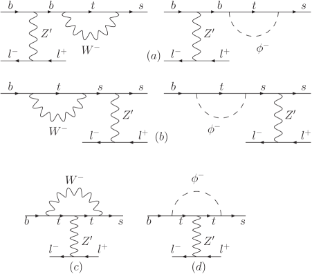
Figure 1: Penguin diagrams of $Z^{\prime}$ contributing to $B_{s}\to l^{+}l^{-}$ in the $TC2$ model.

In the TC2 model, the non-universal gauge boson $Z^{\prime}$ can give corrections to the $SM$ function $Y(x)$, which directly determine the coupling constant $R_{A}$. The relevant Feynman diagrams have been shown in Fig.1. In these diagrams, the Goldstone boson $\phi$ is introduced by the ’t Hooft-Feynman gauge, which can cancel the divergence in self-energy diagrams. Because the couplings of $Z^{\prime}WW$, $Z^{\prime}\phi\phi$ and $Z^{\prime}W\phi$ do not exist in the $TC2$ model, the diagrams that including the above couplings are not present. The small interference effects between $Z^{\prime}$ and $Z$ are not considered here. In this situation, the function $Y^{TC}(x_{t})$ for $l=e,\mu$ is obtained as follows:

$$Y^{TC}(x_{t}) = \frac{-tan^{2}\theta^{\prime}M_{Z}^{2}}{M_{Z^{\prime}}^{2}}\left(C_{ab}(x_{t})+C_{c}(x_{t})+C_{d}(x_{t})\right),$$ (12)

here $x_{t}=m_{t}^{*2}/M_{W}^{2}$. The factor $-tan^{2}\theta^{\prime}$ does not exist for the decay process $B_{s}\to\tau^{+}\tau^{-}$ which can be seen from Eq. (8). The formations of $C_{ab}(x_{t})$, $C_{c}(x_{t})$ and $C_{d}(x_{t})$ can be easily obtained in the framework of the $TC2$ model using the method in Reference [32]. The detailed expression forms of these functions are listed in the Appendix B.

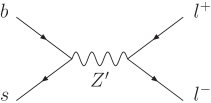
Figure 2: Tree level diagram of $Z^{\prime}$ contributing to $B_{s}\to l^{+}l^{-}$ within the $TC2$ model.

The non-universal gauge boson $Z^{\prime}$ has $FC$ coupling with fermions as shown in Eq. (7), the tree level Feynman diagram contributing to the decay processes $B_{s}\to l^{+}l^{-}$ has been shown in Fig.2. The contributions can be obtained by directly calculating Fig.2 using the standard method in Reference [29], and the $B_{s}$ width can be written as:

$$\Gamma(B_{s}\to l^{+}l^{-})=\frac{1}{4608\,\pi}f_{B_{s}}^{2}m_{B_{s}}m_{l}^{2}\,\sqrt{1-\frac{4m_{l}^{2}}{m_{B_{s}}^{2}}}\,\delta_{bs}^{2}\cot^{2}\theta^{\prime}X^{2}(\theta^{\prime})\left(\frac{g_{1}}{M_{Z^{\prime}}}\right)^{4},$$ (13)

where

$$\delta_{bs}=D_{L}^{bb}D_{L}^{bs*}+2D_{R}^{bb}D_{R}^{bs*}.$$ (14)

$X(\theta^{\prime})=\cot\theta^{\prime}$ for $l=\tau$, and $X(\theta^{\prime})=\tan\theta^{\prime}$ for $l=e$ and $\mu$. $f_{B_{s}}$ is the decay constant of $B_{s}$ meson.

B. The contributions of the scalars ($\pi_{t}^{0,\pm},h^{0}_{t}$)

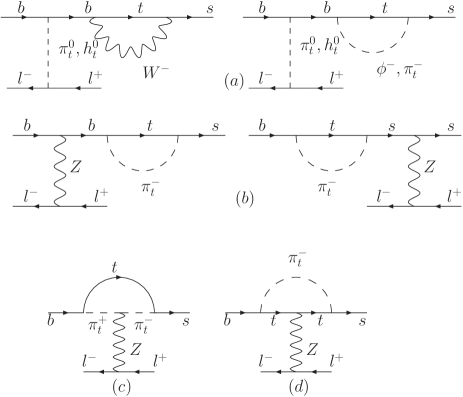
Figure 3: Scalar particles contributing to $B_{s}\to l^{+}l^{-}$ in the $TC2$ model.

The scalars predicted by the $TC2$ model give contributions to the decay processes $B_{s}\to l^{+}l^{-}$ through corrections to the coupling constants in Eq. (10) and Eq. (11). The relevant Feynman diagrams are displayed in Fig.3, in which $(a)$ shows the contributions of neutral top-Higgs $h^{0}_{t}$ and top-pion $\pi_{t}^{0}$ to the couplings $R_{S}$ and $R_{P}$, respectively; $(b)$, $(c)$ and $(d)$ show the contributions of the charged top-pions $\pi_{t}^{\pm}$ to the coupling $R_{A}$. The expression of the coefficient $R_{S}$ can be written as:

$$R_{S}=\frac{\sqrt{\nu_{w}^{2}-F_{\pi}^{2}}}{\nu_{w}}\left(\frac{m_{b}^{*}m_{l}\nu}{2\sqrt{2}sin^{2}\theta_{w}F_{\pi}m_{h_{t}^{0}}^{2}}C(x_{t})+\frac{V_{ts}m_{l}m_{t}^{*}m_{b}^{*2}M_{W}^{2}}{4\sqrt{2}\nu g_{2}^{4}F_{\pi}^{3}m_{h_{t}^{0}}^{2}}C(x_{s})\right).$$ (15)

Here $x_{s}={m^{*}_{t}}^{2}/M_{S}^{2}$, $M_{S}$ is the mass of the top-pions and $g_{2}$ is the $SU(2)$ coupling constant. $C(x_{t})$ is the Inami-Lim function in the $SM$ [32]. Since the neutral top-Higgs coupling with fermions is different from that of neutral top-pion by only a factor of $\gamma_{5}$, the expression of $R_{P}$ is same as that of $R_{S}$ except only for the masses of the scalar particles. In our numerical estimation, we will take $m_{\pi_{t}^{0}}=m_{h_{t}^{0}}=M_{S}$. In this case, $R_{P}=R_{S}$.

The charged top-pions $\pi^{\pm}$ give contributions to the $SM$ function $Y(x)$ via the diagrams $(b)$, $(c)$ and $(d)$ in Fig.3, the expression of the function $Y^{TC}(x_{s})$ can be written as:

$$Y^{TC}(x_{s}) = \frac{1}{4\sqrt{2}G_{F}F_{\pi}^{2}}\left[-\frac{x_{s}^{3}}{8(1-x_{s})}-\frac{x_{s}^{3}}{8(1-x_{s})^{2}}lnx_{s}\right].$$ (16)

C. Numerical results

The branching ratios of the decay processes $B_{s}\to l^{+}l^{-}$ can be written as[3]:

$$Br(B_{s}\rightarrow l^{+}\,l^{-})=a_{s}\left[\left|2m_{l}R_{A}-\frac{m_{B_{s}}^{2}}{m_{b}+m_{s}}R_{P}\right|^{2}+\left(1-\frac{4m_{l}^{2}}{m_{B_{s}}^{2}}\right)\left|\frac{m_{B_{s}}^{2}}{m_{b}+m_{s}}R_{S}\right|^{2}\right]\;,$$ (17)

where

$$a_{s}\equiv\frac{G_{F}^{2}\alpha^{2}}{64\pi^{3}}\,\left|V_{ts}^{\ast}V_{tb}\,\right|^{2}\tau_{B_{s}}f_{B_{s}}^{2}m_{B_{s}}\,\sqrt{1-\frac{4m_{l}^{2}}{m_{B_{s}}^{2}}}\;.$$ (18)

Here $\tau_{B_{s}}$ is the lifetime of $B_{s}$.

The longitudinal polarization asymmetry of the final leptons in $B_{s}\to l^{+}l^{-}$ is defined as follows [3]:

$$A_{LP}^{\pm}\equiv\frac{\left[\Gamma(s_{l^{-}},s_{l^{+}})+\Gamma(\mp s_{l^{-}},\pm s_{l^{+}})\right]-\left[\Gamma(\pm s_{l^{-}},\mp s_{l^{+}})+\Gamma(-s_{l^{-}},-s_{l^{+}})\right]}{\left[\Gamma(s_{l^{-}},s_{l^{+}})+\Gamma(\mp s_{l^{-}},\pm s_{l^{+}})\right]+\left[\Gamma(\pm s_{l^{-}},\mp s_{l^{+}})+\Gamma(-s_{l^{-}},-s_{l^{+}})\right]}\;,$$ (19)

$s_{l^{\pm}}$ are defined into one direction in dilepton rest frame as $(0,\pm\frac{p_{-}}{|p_{-}|})$. For only one direction, there are no difference between the final leptons, thus there is $A_{LP}^{+}=A_{LP}^{-}\equiv A_{LP}$. Then the $A_{LP}$ can be written as:

$$A_{LP}(B_{s}\to l^{+}l^{-})=\frac{2\sqrt{1-\frac{4m_{l}^{2}}{m_{B_{s}}^{2}}}Re\left[\frac{m_{B_{s}}^{2}}{m_{b}+m_{s}}R_{S}\left(2m_{l}R_{A}-\frac{m_{B_{s}}^{2}}{m_{b}+m_{s}}~{}R_{P}\right)\right]}{\left|2m_{l}R_{A}-\frac{m_{B_{s}}^{2}}{m_{b}+m_{s}}R_{P}\right|^{2}+(1-\frac{4m_{l}^{2}}{m_{B_{s}}^{2}})\left|\frac{m_{B_{s}}^{2}}{m_{b}+m_{s}}R_{S}\right|^{2}}.$$ (20)

$A_{LP}^{SM}(B_{s}\to l^{+}l^{-})\simeq 0$ because $R_{S}\sim{\cal O}(10^{-5})$ in the $SM$.

$$G_{F}=1.166\times 10^{-5}\;{\rm GeV}^{-2}$$

[33]

Table 1: Numerical inputs used in our analysis. Unless explicitly specified, they are                taken from the Particle Data Group [34].

Before giving numerical results, we need to specify the relevant $SM$ parameters. These parameters have mainly been shown in Table 1. We take the coupling constant $K_{1}$, the model dependent parameter $\varepsilon$, the mass of non-universal gauge boson $M_{Z^{\prime}}$ and the mass of scalars $M_{S}$ as free parameters in our numerical estimation. The value of $M_{S}$ remains subject to large uncertainty [20]. However, it has been shown that its value is generally allowed to be in the range of a few hundred $\rm GeV$ depending on the models [21]. In our numerical estimation, we will assume that $M_{S}$ is in the range of $200\rm GeV\sim\rm 500GeV$. The lower bounds on $M_{Z^{\prime}}$ can be obtained from dijet and dilepton production in the Tevatron experiments [22] or $B\bar{B}$ mixing [23]. However, these bounds are significantly weaker than those from the precision electroweak data. Reference [24] has shown that, to fit the precision electroweak data, the $Z^{\prime}$ mass $M_{Z^{\prime}}$ must be larger than $1\ TeV$. In our numerical estimation, we will assume that the values of the free parameters $\varepsilon$, $K_{1}$ and $M_{Z^{\prime}}$ are in the range of $0.03\sim 0.1$, $0\sim 1$ and $1000\ \rm GeV\ \sim 2000\ \rm GeV$, respectively.

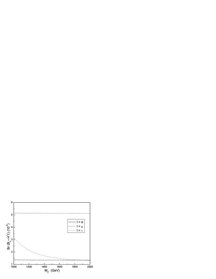
(a) $K_{1}=0.4$

(b) $K_{1}=0.8$

Figure 4: The branching ratios of $B_{s}\to l^{+}l^{-}$ as function of the parameter $M_{Z^{\prime}}$                 for $K_{1}=0.4$ (a) and $K_{1}=0.8$ (b).

First we give our numerical results of the decay processes $B_{s}\to l^{+}l^{-}$ induced by the non-universal gauge boson $Z^{\prime}$. The branching ratios of $B_{s}\to l^{+}l^{-}$ are plotted in Fig.4 as function of the mass parameter $M_{Z^{\prime}}$ for $K_{1}=0.4$ and $0.8$, in which we have multiplied the factors $10^{7}$ and $10^{3}$ to the values of $Br(B_{s}\to e^{+}e^{-})$ and $Br(B_{s}\to\mu^{+}\mu^{-})$, respectively. From these figures one can see that the values of $Br(B_{s}\to\tau^{+}\tau^{-})$ are sensitive to the mass of $Z^{\prime}$, they increase as the mass parameter $M_{Z^{\prime}}$ decreasing. For $l=e,\mu$, the values of their branching ratios are not so sensitive to the parameter $M_{Z^{\prime}}$. Because the contributions of $Z^{\prime}$ to $Br(B_{s}\to e^{+}e^{-})$ and $Br(B_{s}\to\mu^{+}\mu^{-})$ are small relative to the $SM$ contributions. The values of the corresponding branching ratios are both below ${\cal O}(10^{-9})$ which are not easy to be observed in current collider experiments. The contributions of $Z^{\prime}$ to the branching ratio of the decay $B_{s}\to\tau^{+}\tau^{-}$ are large, since the non-universal gauge boson $Z^{\prime}$ has large couplings to the third generation fermion with respect to the first two generations, it can make the branching ratio value reach ${\cal O}(10^{-6})$ with reasonable values of the free parameters.

(a) $\varepsilon=0.04$

(b) $\varepsilon=0.08$

Figure 5: The branching ratios of $B_{s}\to l^{+}l^{-}$ as function of the parameter $M_{S}$ for                 $\varepsilon=0.04$ (a) and $\varepsilon=0.08$ (b).

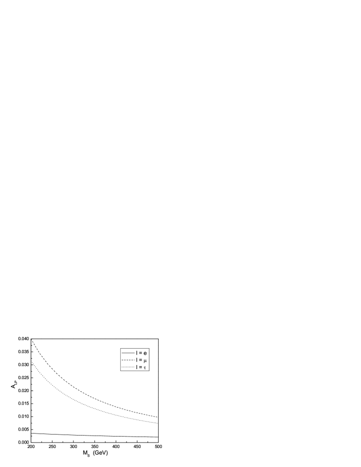
(a) $\varepsilon=0.04$

(b) $\varepsilon=0.08$

Figure 6: The longitudinal polarization asymmetry in $B_{s}\to l^{+}l^{-}$ as function of the                 parameter $M_{S}$ for $\varepsilon=0.04$ (a) and $\varepsilon=0.08$ (b).

The branching ratios of $B_{s}\to l^{+}l^{-}$ contributed by the scalars ($\pi_{t}^{0,\pm}$ and $h_{t}^{0}$) are plotted in Fig.5 as function of the mass parameter $M_{S}$ for $\varepsilon=0.04$ and $0.08$, in which we have multiplied the factors $10^{7}$ and $10^{2}$ to the values of $Br(B_{s}\to e^{+}e^{-})$ and $Br(B_{s}\to\mu^{+}\mu^{-})$, respectively. It is obvious that the values of the branching ratios for these decays increase as the parameter $M_{S}$ decreasing. Furthermore, the enhancement to the branching ratio of the decay process $B_{s}\to\mu^{+}\mu^{-}$ is larger than that of the $Z^{\prime}$ contributions by an order of magnitude.

The value of $Br(B_{s}\to e^{+}e^{-})$ is smaller than that of $Br(B_{s}\to\mu^{+}\mu^{-})$ by five orders of magnitude, which is because it is suppressed by $m_{e}^{2}/m_{\mu}^{2}$ with respect to $\mu$ channel. The branching ratio for $\tau^{+}\tau^{-}$ mode is enhanced by a factor of $10^{2}$ to $\mu$ channel, its value can reach ${\cal O}(10^{-6})$ by our calculation. However, the $\tau^{+}\tau^{-}$ channel is still not easy to be observed under present experimental precision, while the current experimental upper limit for $Br(B_{s}\to\tau^{+}\tau^{-})$ from the BARBAR collaboration is $4.1\times 10^{-3}$ at $90\%~{}\rm{C.L.}$ [35]. So the experimental searches for $B_{s}\to l^{+}l^{-}$ have focused on the $\mu$ channel, and we only discuss this channel. Comparing with the $SM$ prediction $Br(B_{s}\to\mu^{+}\mu^{-})=3.86\pm 0.15\times 10^{-9}$ [1], the contributions of the new scalars predicted by the $TC2$ model can enhance this value by one order of magnitude, so our results are more approach to the experimental data given by Eq. (1).

Obviously, the non-universal gauge boson $Z^{\prime}$ has no contributions to the $SPNP$ operators, so it was not considered in this subsection. The longitudinal polarization asymmetry $A_{LP}$ contributed by the new scalars predicted by the $TC2$ model as function of the parameter $M_{S}$ are plotted in Fig.6. From these figures one can see that the $A_{LP}$ is sensitive to the mass of the scalars, especially for $l=\mu,\tau$, however it is less sensitive to the parameter $\varepsilon$. The values of the asymmetry $A_{LP}$ can reach nearly $4\%$ for $l=\mu,\tau$ when the mass of the scalars get to $200\rm~{}GeV$.

IV. The contributions of the $\rm{TC2}$ model to the rare decay processes      $B\to Kl^{+}l^{-}$

The effective Hamilton for the decay $B\to Kl^{+}l^{-}$ is similar to that of $B_{s}\to l^{+}l^{-}$ as shown in Eq. (9), which is constituted by two parts. The $SPNP$ part is same as the expression shown in Eq. (11). In the framework of the $TC2$ model, The $H_{0}$ part can be written as [31]:

$$\begin{split}H_{0}&=\frac{\alpha G_{F}}{\sqrt{2}\pi}V_{tb}V^{*}_{ts}\biggl{\{}C^{\rm eff}_{9}(\bar{s}\gamma_{\mu}P_{L}b)\,\bar{l}\gamma_{\mu}l+C_{10}(\bar{s}\gamma_{\mu}P_{L}b)\,\bar{l}\gamma_{\mu}\gamma_{5}l\\ &-2\frac{C^{\rm eff}_{7}}{q^{2}}m_{b}\,(\bar{s}i\sigma_{\mu\nu}q^{\nu}P_{R}b)\,\bar{l}\gamma_{\mu}l\biggr{\}}\,.\end{split}$$ (21)

Here $q_{\mu}$ is the sum of $4$-momenta of $l^{+}$ and $l^{-}$. The Wilson coefficients $C_{7}^{eff}$, $C_{9}^{eff}$ and $C_{10}$ contain two parts of contributions from the $SM$ and the $TC2$ model.

Similar to the decay processes $B_{s}\to l^{+}l^{-}$, the non-universal gauge boson $Z^{\prime}$ give contributions to the Wilson coefficients $C_{9}^{eff}$ and $C_{10}$, the relevant Feynman diagrams are same as Fig.1 and the relevant functions $Y^{TC}(x_{t})$ and $Z^{TC}(x_{t})$ have same expressions as shown in Eq. (12).

The charged top-pions $\pi_{t}^{\pm}$ can give contributions to the Wilson coefficients $C_{7}^{eff}$ and $C_{9}^{eff}$. The relevant Feynman diagrams are similar to Fig.3. However, these penguin diagrams are induced by $\gamma$ penguins, gluon penguins and chromomagnetic penguins. The coefficients $C_{7}^{eff}$ and $C_{9}^{eff}$ can be expressed in terms of the corresponding functions $D_{1}(x_{s})$, $E_{1}(x_{s})$ and $E_{1}^{\prime}(x_{s})$, which are added to the corresponding $SM$ functions $D_{0}(x_{t})$, $E_{0}(x_{t})$ and $E_{0}^{\prime}(x_{t})$ [32]. The detailed expression forms of the these functions are [36]:

$$D_{1}(x) = \frac{1}{4\sqrt{2}G_{F}F_{\pi}}\left(\frac{47-79x+38x^{2}}{108(1-x)^{3}}+\frac{3-6x^{2}+4x^{3}}{18(1-x)^{4}}ln(x)\right),$$ (22)

$$E_{1}(x) = \frac{1}{4\sqrt{2}G_{F}F_{\pi}}\left(\frac{7-29x+16x^{2}}{36(1-x)^{3}}-\frac{3x^{2}-2x^{3}}{6(1-x)^{4}}ln(x)\right),$$ (23)

$$E_{1}^{\prime}(x) = \frac{1}{8\sqrt{2}G_{F}F_{\pi}}\left(\frac{5-19x+20x^{2}}{6(1-x)^{3}}-\frac{x^{2}-2x^{3}}{(1-x)^{4}}ln(x)\right).$$ (24)

We can obtain the corrected Wilson coefficients $C_{7}^{eff}$, $C_{9}^{eff}$ and $C_{10}$ with these corrected functions using the relevant expressions of these coefficients in References [10, 36], which are listed in Appendix C. The neutral top-pion $\pi_{t}^{0}$ and top-Higgs $h_{t}^{0}$ can also give contributions to these decay processes through the $SPNP$ operators, and the expression forms of $R_{S}$ ($R_{P}$) are same as those shown in Eq. (15).

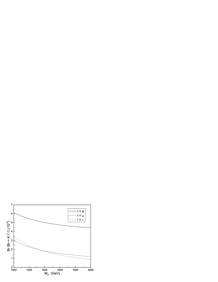
(a) $K_{1}=0.4$

(b) $K_{1}=0.8$

Figure 7: The branching ratios of $B\to Kl^{+}l^{-}$ as function of the parameter $M_{Z^{\prime}}$                 for $K_{1}=0.4$ (a) and $K_{1}=0.8$ (b).

The branching ratios $Br(B\to Kl^{+}l^{-})$ ($l=e,\mu$ and $\tau$) contributed by the gauge boson $Z^{\prime}$ are plotted in Fig.7 as a function of the mass parameter $M_{Z^{\prime}}$ for two values of $K_{1}$, in which we have multiplied the factor $10^{-1}$ and $10^{-2}$ to the branching ratios of decays $B\to K\mu^{+}\mu^{-}$ and $B\to K\tau^{+}\tau^{-}$ respectively. From this figure one can see that the values of the branching ratios for $l=e,\mu$ and $\tau$ increase as the parameter $M_{Z^{\prime}}$ decreasing. However, the branching ratios for $l=e$ are not sensitive to the parameter $M_{Z^{\prime}}$ as shown in these figures. The values of the branching ratios for $l=e$ and $\mu$ are not sensitive to the parameter $K_{1}$. For $K_{1}=0.4$ and $1000\rm GeV\leq M_{Z^{\prime}}\leq 2000\rm GeV$, the values of $Br(B\to Ke^{+}e^{-})$ and $Br(B\to K\mu^{+}\mu^{-})$ are in the range of $6.1\times 10^{-8}\sim 4.4\times 10^{-8}$ and $3.0\times 10^{-7}\sim 1.2\times 10^{-7}$, respectively.

(a) $\varepsilon=0.04$

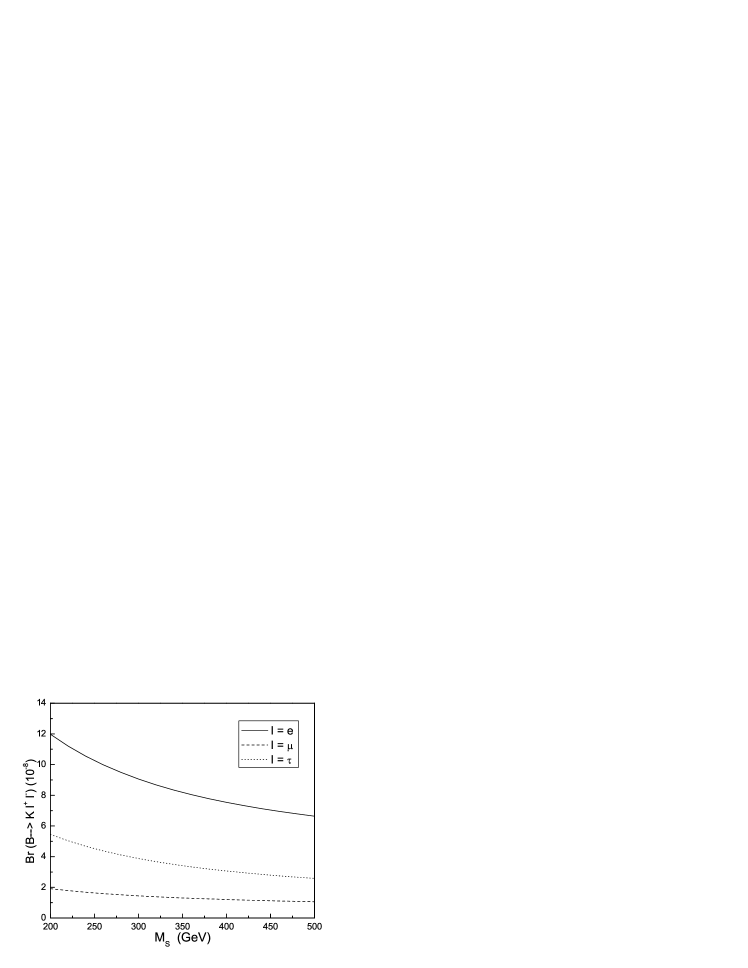
(b) $\varepsilon=0.08$

Figure 8: The branching ratios of $B\to Kl^{+}l^{-}$ as function of the parameter $M_{S}$ for                 $\varepsilon=0.04$ (a) and $\varepsilon=0.08$ (b).

The branching ratios of the decay processes $B\to Kl^{+}l^{-}$ contributed by the scalars ($\pi_{t}^{0,\pm},h_{t}^{0}$) are plotted in Fig.8 as function of the mass parameter $M_{S}$ for $\varepsilon=0.04$ and $0.08$, in which we have multiplied the factors $10^{-1}$ to the branching ratio of $B\to K\mu^{+}\mu^{-}$. From these figures, one can see that the values of the branching ratios of these decay processes increase as the parameter $M_{S}$ decreasing. All of their values are not sensitive to the parameter $\varepsilon$. The contributions of the scalars for $l=e$ and $\mu$ are comparable to those of the non-universal gauge boson $Z^{\prime}$, the values of the branching ratios of $B\to Ke^{+}e^{-}$ and $B\to K\mu^{+}\mu^{-}$ contributed by both the scalars and the non-universal gauge boson can reach ${\cal O}(10^{-7})$, which give an explanation to the deviation between the experimental data and the $SM$ predictions in Reference [8]. While the scalar’s contribution to the decay process $B\to K\tau^{+}\tau^{-}$ is smaller than that of the non-universal gauge boson $Z^{\prime}$ by two order of magnitude and therefore can be neglected. When the $Z^{\prime}$ mass is in the range of $1000\rm~{}GeV\sim 2000\rm~{}GeV$, the values of $Br(B\to K\tau^{+}\tau^{-})$ are in the range of $7.0\times 10^{-6}\sim 1.7\times 10^{-6}$. This result is 2 orders of magnitude larger than the $e$ and $\mu$ channel, which is because of the large coupling of $Z^{\prime}$ to the third generation fermions.

The normalized forward-backward ($FB$) asymmetry can be defined as [4]:

$$A_{FB}(z)=\frac{\int_{0}^{1}dcos\theta\frac{d^{2}\Gamma}{dzdcos\theta}-\int_{-1}^{0}dcos\theta\frac{d^{2}\Gamma}{dzdcos\theta}}{\int_{0}^{1}dcos\theta\frac{d^{2}\Gamma}{dzdcos\theta}+\int_{-1}^{0}dcos\theta\frac{d^{2}\Gamma}{dzd\cos\theta}}\;.$$ (25)

After the integral calculation of $FB$ asymmetry gives,

$$\langle A_{FB}\rangle=\frac{2\tau_{B}\Gamma_{0}\,\hat{m}_{l}\,\beta_{\mu}^{2}\,R_{S}\,\int dz\,a_{1}(z)\,\phi(1,k^{2},z)}{Br(B\to Kl^{+}l^{-})}\;,$$ (26)

where $\tau_{B}$ is the lifetime of $B$ meson and $Br(B\to Kl^{+}l^{-})$ is the total branching ratio of $B\to Kl^{+}l^{-}$ and $\Gamma_{0}$ is the total width of the $B$ meson, which can be written as:

$$\Gamma_{0}=\frac{G_{F}^{2}\alpha^{2}}{2^{9}\pi^{5}}\,|V_{tb}V_{ts}^{*}|^{2}\,m_{B}^{5}\;,$$ (27)

$$a_{1}(z)=\frac{1}{2}(1-k^{2})C_{9}f_{0}(z)f_{+}(z)+(1-k)C_{7}f_{0}(z)f_{T}(z)\;.$$ (28)

Other relevant functions such as $\phi(1,k^{2},z)$ are listed in Appendix C. The form factors $f_{+}$, $f_{0}$ and $f_{T}$ are defined in the relevant matrix elements as:

$$\left<K(p^{\prime})\left|\bar{s}\gamma_{\mu}b\right|B(p)\right> = (2p-q)_{\mu}f_{+}(z)+(\frac{1-k^{2}}{z})\,q_{\mu}[f_{0}(z)-f_{+}(z)]\;,$$ (29)

$$\left<K(p^{\prime})\left|\bar{s}i\sigma_{\mu\nu}q^{\nu}b\right|B(p)\right> = -\Big{[}(2p-q)_{\mu}q^{2}-(m_{B}^{2}-m_{K}^{2})q_{\mu}\Big{]}\,\frac{f_{T}(z)}{m_{B}+m_{K}}\;,$$ (30)

$$\left<K(p^{\prime})\left|\bar{s}b\right|B(p)\right> = \,\frac{m_{B}(1-k^{2})}{\hat{m}_{b}}\,f_{0}(z)\;.$$ (31)

Here, $k\equiv m_{K}/m_{B}$, $z\equiv q^{2}/m_{B}^{2}$ and $\hat{m}_{b}\equiv m_{b}/m_{B}$. The form factors $f_{+}$, $f_{0}$ and $f_{T}$ can be calculated by using the light cone $QCD$ approach. Their particular forms can be found in Reference [31]. In this paper, we assume $\hat{m}_{b}\doteq 1$.

(a) $\varepsilon=0.04$

(b) $\varepsilon=0.08$

Figure 9: In the $TC2$ model, the forward-backward asymmetry in $B\to Kl^{+}l^{-}$ as                 function of $M_{S}$ for the parameter $\varepsilon=0.04$ (a) and $\varepsilon=0.08$ (b).

The production of the $FB$ asymmetries are only sensitive to $SPNP$ operators. From Eq. (26), one can see that the non-universal gauge boson $Z^{\prime}$ has no contribution to the $FB$ asymmetry, so we only discuss the contributions coming from the scalars ($\pi_{t}^{0,\pm},h_{t}^{0}$).

The $FB$ asymmetry $A_{FB}$ of leptons in the decay processes $B\to Kl^{+}l^{-}$ are plotted in Fig.9 as function of the parameter $M_{S}$ for $\varepsilon=0.04$ and $0.08$, in which we have multiplied the factors $10^{5}$ and $10$ to the value of $A_{FB}(B\to Ke^{+}e^{-})$ and $A_{FB}(B\to K\mu^{+}\mu^{-})$ respectively. From this figure one can see that the value of $A_{FB}$ is smaller than ${\cal O}(10^{-3})$ in most of the parameter spaces. Comparing its experimental measurement value, this value is not large enough to be observed in experiments. One can see that the contributions of the $TC2$ model to the $FB$ asymmetry in these decay processes are smaller than those of the $SUSY$ models. Considering the uncertainty in measurements, it is very difficult to detect the signals of the $TC2$ model through measuring the $FB$ asymmetry about these decay processes.

V. The contributions of the $\rm{LHT}$ model to the rare decay processes      $b\to sl^{+}l^{-}$

The $LHT$ model [14] is based on an $SU(5)/SO(5)$ global symmetry breaking pattern. A subgroup $[SU(2)\times U(1)]_{1}\times[SU(2)\times U(1)]_{2}$ of the $SU(5)$ global symmetry is gauged, and at the scale $f$ it is broken into the $SM$ electroweak symmetry $SU(2)_{L}\times U(1)_{Y}$. T-parity is an automorphism which exchanges the $[SU(2)\times U(1)]_{1}$ and $[SU(2)\times U(1)]_{2}$ gauge symmetries. The T-even combinations of the gauge fields are the $SM$ electroweak gauge bosons $W_{\mu}^{a}$ and $B_{\mu}$. The T-odd combinations are T-parity partners of the $SM$ electroweak gauge bosons.

After taking into account $EWSB$, at the order of $\nu^{2}/f^{2}$, the masses of the T-odd set of the $SU(2)\times U(1)$ gauge bosons are given as:

$$M_{B_{H}}=\frac{g^{\prime}f}{\sqrt{5}}[1-\frac{5\nu^{2}}{8f^{2}}],\hskip 14.22636ptM_{Z_{H}}\approx M_{W_{H}}=gf[1-\frac{\nu^{2}}{8f^{2}}],$$ (32)

where $f$ is the scale parameter of the gauge symmetry breaking of the $LHT$ model. $g^{\prime}$ is the $SM$ $U(1)_{Y}$ gauge coupling constants. Because of the smallness of $g^{\prime}$, the T-odd gauge boson $B_{H}$ is the lightest T-odd particle, which can be seen as an attractive dark matter candidate [37]. To avoid severe constraints and simultaneously implement T-parity, it is necessary to double the $SM$ fermion doublet spectrum [14, 38]. The T-even combination is associated with the $SU(2)_{L}$ doublet, while the T-odd combination is its T-parity partner. The masses of the T-odd fermions can be written in a unified manner as:

$$M_{F_{i}}=\sqrt{2}k_{i}f,$$ (33)

where $k_{i}$ are the eigenvalues of the mass matrix $k$ and their values are generally dependent on the fermion species $i$.

The mirror fermions (T-odd quarks and T-odd leptons) have new flavor violating interactions with the $SM$ fermions mediated by the new gauge bosons $(B_{H},W_{H}^{\pm}$, or $Z_{H})$, which are parametrized by four $CKM$-like unitary mixing matrices, two for mirror quarks and two for mirror leptons [39, 40]:

$$V_{Hu},\hskip 5.69046ptV_{Hd},\hskip 5.69046ptV_{Hl},\hskip 5.69046ptV_{H\nu}.$$ (34)

They satisfy:

$$V_{Hu}^{+}V_{Hd}=V_{CKM},\hskip 5.69046ptV_{H\nu}^{+}V_{Hl}=V_{PMNS}.$$ (35)

Where the $CKM$ matrix $V_{CKM}$ is defined through flavor mixing in the down-type quark sector, while the $PMNS$ matrix $V_{PMNS}$ is defined through neutrino mixing.

The contributions of the $LHT$ model to the rare decay processes $b\to sl^{+}l^{-}$ are mainly coming from the corrections to the Wilson coefficients, which related to the $SM$ Inami-Lim functions [32]. The branching ratios of the decay processes $B_{s}\to l^{+}l^{-}$ in the $SM$ depend on a function $Y_{SM}$ and the $LHT$ effects enter through the modification of the function $Y_{SM}$ [39]. With the $LHT$ effects $Y_{SM}$ is replaced by [15]:

$$Y_{s}=Y_{SM}+\bar{Y}^{\rm even}+\frac{\bar{Y}_{s}^{\rm odd}}{\lambda_{t}^{(s)}},$$ (36)

where $\bar{Y}^{\rm even}$ and $\bar{Y}_{s}^{\rm odd}$ represent the effects from T-even and T-odd particles, respectively. The branching ratios normalized to the $SM$ predictions are then given by:

$$\frac{Br(B_{s}\to l^{+}l^{-})}{Br(B_{s}\to l^{+}l^{-})_{\text{SM}}}=\left|\frac{Y_{s}}{Y_{\text{SM}}}\right|^{2},$$ (37)

which $Br(B_{s}\to l^{+}l^{-})_{\text{SM}}$ are the branching ratios predicted by the $SM$. Their particular numerical values of the branching ratios for the decay processes $B_{s}\to l^{+}l^{-}$ in the $LHT$ model are listed as follows:

$$Br(B_{s}\to e^{+}e^{-}) = (1.36\pm 0.05)\times 10^{-13},$$ (38)

$$Br(B_{s}\to\mu^{+}\mu^{-}) = (5.79\pm 0.23)\times 10^{-9},$$ (39)

$$Br(B_{s}\to\tau^{+}\tau^{-}) = (1.23\pm 0.05)\times 10^{-6}.$$ (40)

The branching ratios of the decay processes $B\to Kl^{+}l^{-}$ in the $SM$ depend on the functions $Y_{SM}$, $Z_{SM}$ and $D_{0}^{\prime}(x_{t})$ ($D_{0}^{\prime}(x_{t})$ is same as in $B\to X_{s}\gamma$ [15]), the $LHT$ effects enter through the modification of these functions. The modifications of the function $Y_{SM}$ has been given above, and the modifications of the function $Z_{SM}$ is given by [15, 39]:

$$Z_{s}=Z_{SM}+\bar{Z}^{\rm even}+\frac{\bar{Z}_{s}^{odd}}{\lambda_{t}^{(s)}},$$ (41)

where $\bar{Z}^{\rm even}$ and $\bar{Z}_{s}^{odd}$ represent the effects coming from T-even and T-odd particles, respectively. Similar with Sec. IV, we can calculate the contributions of the $LHT$ model to the decay processes $B\to Kl^{+}l^{-}$. With reasonable values of the free parameters in the framework of the $LHT$ model, the maximum values of the branching ratios for the rare decays $B\to Kl^{+}l^{-}$ are:

$$Br(B\to Ke^{+}e^{-}) = 9.66\times 10^{-6},$$ (42)

$$Br(B\to K\mu^{+}\mu^{-}) = 6.56\times 10^{-6},$$ (43)

$$Br(B\to K\tau^{+}\tau^{-}) = 2.99\times 10^{-7}.$$ (44)

These numerical results are obtained by calculating the relative correction to the $SM$ predictions in the framework of the $LHT$ model, while the $SM$ predictions exist the uncertainty coming from the next-to-leading logarithmic ($NLO$) contributions and the long-distance contributions, for which the $Br(B\to Kl^{+}l^{-})$ are a little disparity away from their respective experimental upper limits [41]. However, there is no disagreement with experiment in some parameter ranges while the corrected effects is no more than 15 percent.

The contributions of the $LHT$ model to the asymmetry observables $A_{FB}$ and $A_{LP}$ in the rare decay processes $b\to sl^{+}l^{-}$ mainly come from the new neutral scalar particles. For the $B_{s}$ meson, there is an unitarity relation of the $V_{Hd}$ matrix [39]:

$$\xi^{(s)}_{1}+\xi^{(s)}_{2}+\xi^{(s)}_{3}=0,$$ (45)

where $\xi^{(s)}_{i}=V_{Hd}^{*ib}V_{Hd}^{is}$. Considering this relation, the calculations of the relevant Feynman diagrams similar to Fig.3 equal to zero. Hence, in the framework of the $LHT$ model, the total contributions induced by the neutral scalars equal to zero. The contributions to the $A_{FB}$ and $A_{LP}$ is close to the predictions in the $SM$.

VI. Conclusions

The $SM$ is a very successful theory but it can only be an effective theory below some high energy scales. To completely avoid the problems arising from the elementary Higgs field in the $SM$, various kinds of dynamical electroweak symmetry breaking models have been proposed, among which the topcolor scenario is attractive because it can explain the large top quark mass and provide a possible $EWSB$ mechanism. The $TC2$ model has all essential features of the topcolor scenario. It is expected that the possible signals of the $TC2$ model should be detected in the future high energy collider experiments.

In this paper we consider the contributions of the $TC2$ model to observables related to the decay processes $B_{s}\to l^{+}l^{-}$ and $B\to Kl^{+}l^{-}$. We find that the $TC2$ model can enhance the branching ratios of the $SM$ predictions for these decay processes $B_{s}\to l^{+}l^{-}$ and $B\to Kl^{+}l^{-}$. In wide ranges of the free parameter space, it is possible to enhance the values of $Br(B_{s}\to l^{+}l^{-})$ and $Br(B\to Kl^{+}l^{-})$ by one order of magnitude. In the $TC2$ model, the non-universal gauge boson $Z^{\prime}$ gives main contributions to $Br(B_{s}\to\tau^{+}\tau^{-})$, while the contributions of $Z^{\prime}$ to $Br(B_{s}\to e^{+}e^{-})$ and $Br(B_{s}\to\mu^{+}\mu^{-})$ are comparable with those of the new scalars ($\pi_{t}^{0,\pm},h_{t}^{0}$). For the decay processes $B\to Ke^{+}e^{-}$ and $B\to K\mu^{+}\mu^{-}$, the contributions of $Z^{\prime}$ are comparable with those of the scalars. While the contributions of the $TC2$ model to $Br(B\to K\tau^{+}\tau^{-})$ mainly come from $Z^{\prime}$.

The production of the asymmetries are only sensitive to $SPNP$ operators, so there are no contributions of $Z^{\prime}$ to the relevant observables. We further calculate the contributions of the new scalars predicted by the $TC2$ model to the asymmetry observables $A_{FB}$ and $A_{LP}$ of leptons in the decay processes $B_{s}\to l^{+}l^{-}$ and $B\to Kl^{+}l^{-}$. Our numerical results show that, when the mass of the scalars gets to $200\rm GeV$, the values of the asymmetry $A_{LP}$ in the decay processes $B_{s}\to\mu^{+}\mu^{-}$ and $B_{s}\to\tau^{+}\tau^{-}$ can reach $4\%$ . We hope that the values of $A_{LP}$ for $l=\mu,\tau$ can approach the detectability threshold of the near future experiments. However, the contributions of these new scalars to $A_{FB}$ are around ${\cal O}(10^{-4})$ in most of the parameter space, which are not large enough to be detected.

The $LHT$ model is one of the attractive little Higgs models, which satisfies the electroweak precision data in most of the parameter space. This model can produce rich phenomenology at present and in future high energy experiments. New particles predicted by this model give contributions to the branching ratios of the rare decay processes $B_{s}\to l^{+}l^{-}$ and $B\to Kl^{+}l^{-}$. Reference [15] has shown that, comparing with their $SM$ predictions, the branching ratios of the decay processes $B_{s}\to l^{+}l^{-}$ and $B\to Kl^{+}l^{-}$ can be enhanced by at most $50\%$ and $15\%$, respectively. For comparison, we give a brief description and particular numerical results about these rare decays. In addition, we show that the neutral scalars predicted by this model can not give contributions to the asymmetry observables $A_{FB}$ and $A_{LP}$.

In conclusion, the effects of the $TC2$ model on the branching ratios and asymmetry observables related to the rare decay processes $b\to sl^{+}l^{-}$ can give positive contributions to the $SM$ predictions. The numerical results show that the branching ratios for these decays are much close to the experimental data, such as $Br(B_{s}\to\mu^{+}\mu^{-})$. The value of $Br(B\to K\tau^{+}\tau^{-})$ is larger than the $SM$ prediction by one order of magnitude, which is hoped to be observed in the future high accuracy experiments, or the future experimental results may give constraints on the free parameters of the $TC2$ model. Hence, it is indicated that the possible signals of the $TC2$ model may be observed through the above decay processes in future experiments.

Acknowledgments

This work was supported in part by the National Natural Science Foundation of China under Grants No.10675057, Specialized Research Fund for the Doctoral Program of Higher Education(SRFDP) (No.200801650002), the Natural Science Foundation of the Liaoning Scientific Committee(No.20082148), and Foundation of Liaoning Educational Committee(No.2007T086).

Appendix

A. Relevant functions in the $SM$

In this Appendix we list the functions in the $SM$ that entered the present study of rare B decays.

$$Y^{SM}(x) = \frac{1}{8}\left[\frac{x-4}{x-1}+\frac{3x}{(x-1)^{2}}\ln x\right],$$ (46)

$$Z^{SM}(x_{t}) = -\frac{1}{9}\ln x_{t}+\frac{18x_{t}^{4}-163x_{t}^{3}+259x_{t}^{2}-108x_{t}}{144(x_{t}-1)^{3}}$$ (47)

$$+\frac{32x_{t}^{4}-38x_{t}^{3}-15x_{t}^{2}+18x_{t}}{72(x_{t}-1)^{4}}\ln x_{t}\,,$$

$$D_{0}(y) = -\frac{4}{9}\ln y+\frac{-19y^{3}+25y^{2}}{36(y-1)^{3}}+\frac{y^{2}(5y^{2}-2y-6)}{18(y-1)^{4}}\ln y\,,$$ (48)

$$E_{0}(y) = -\frac{2}{3}\ln y+\frac{y^{2}(15-16y+4y^{2})}{6(y-1)^{4}}\ln y+\frac{y(18-11y-y^{2})}{12(1-y)^{3}}\,,$$ (49)

$$D^{\prime}_{0}(y) = -\dfrac{(3y^{3}-2y^{2})}{2(y-1)^{4}}\ln y+\dfrac{(8y^{3}+5y^{2}-7y)}{12(y-1)^{3}}\,,$$ (50)

$$E^{\prime}_{0}(y) = \dfrac{3y^{2}}{2(y-1)^{4}}\ln y+\dfrac{(y^{3}-5y^{2}-2y)}{4(y-1)^{3}}\,.$$ (51)

B. Relevant functions in the TC2 model

In this Appendix we list the functions that entered the present study of rare B decays in the framework of the TC2 model.

$$C_{ab}(x) = -\frac{2g^{2}c_{w}^{2}F_{1}(x)}{3g_{2}^{2}(v_{d}+a_{d})},$$ (52)

$$C_{c}(x) = \frac{2f^{2}c_{w}^{2}}{g_{2}^{2}}\left(\frac{2F_{2}(x)}{3(v_{u}+a_{u})}+\frac{F_{3}(x)}{6(v_{u}-a_{u})}\right),$$ (53)

$$C_{d}(x) = \frac{2f^{2}c_{w}^{2}}{g_{2}^{2}}\left(\frac{2F_{4}(x)}{3(v_{u}+a_{u})}+\frac{F_{5}(x)}{6(v_{u}-a_{u})}\right),$$ (54)

$$C(x) = \frac{F_{1}(x)}{-(0.5(Q-1)s_{w}^{2}+0.25)}.$$ (55)

Here the variables are defined as: $g=\sqrt{4\pi K_{1}}$, $v_{u,d}=I_{3}-2Q_{u,d}s_{w}^{2}$, $s_{w}=\sin\theta_{w}$, $a_{u,d}=I_{3}$, where $u,d$ represent the up and down type quarks, respectively.

$$F_{1}(x) = -(0.5(Q-1)s_{w}^{2}+0.25)(x^{2}ln(x)/(x-1)^{2}-x/(x-1)-x(0.5(-0.5772$$ (56)

$$+ ln(4\pi)-ln(M_{W}^{2}))+0.75-0.5(x^{2}ln(x)/(x-1)^{2}-1/(x-1)))),$$

$$F_{2}(x) = (0.5Qs_{w}^{2}-0.25)(x^{2}ln(x)/(x-1)^{2}-2xln(x)/(x-1)^{2}+x/(x-1)),$$ (57)

$$F_{3}(x) = -Qs_{w}^{2}(x/(x-1)-xln(x)/(x-1)^{2}),$$ (58)

$$F_{4}(x) = 0.25(4s_{w}^{2}/3-1)(x^{2}ln(x)/(x-1)^{2}-x-x/(x-1)),$$ (59)

$$F_{5}(x) = -0.25Qs_{w}^{2}x(-0.5772+ln(4\pi)-ln(M_{W}^{2})+1-xln(x)/(x-1))$$ (60)

$$- s_{w}^{2}/6(x^{2}ln(x)/(x-1)^{2}-x-x/(x-1)).$$

C. Relevant expressions in our calculation

In this Appendix we list the functions that entered the present study of rare B decays and some expressions of the relevant coefficients.

$$M\,(B\rightarrow Kl^{+}l^{-}) = \frac{\alpha G_{F}}{2\sqrt{2}\pi}V_{tb}V^{*}_{ts}$$ (61)

$$\times \Bigg{[}\left<K(p^{\prime})\left|\bar{s}\gamma_{\mu}b\right|B(p)\right>\left\{C_{9}^{\rm eff}\bar{u}(p_{+})\gamma_{\mu}v(p_{-})+C_{10}\bar{u}(p_{+})\gamma_{\mu}\gamma_{5}v(p_{-})\right\}$$

$$-2\frac{C^{\rm eff}_{7}}{q^{2}}m_{b}\left<K(p^{\prime})\left|\bar{s}i\sigma_{\mu\nu}q^{\nu}b\right|B(p)\right>\bar{u}(p_{+})\gamma_{\mu}v(p_{-})$$

$$+\left<K(p^{\prime})\left|\bar{s}b\right|B(p)\right>\left\{R_{S}\bar{u}(p_{+})v(p_{-})+R_{P}\bar{u}(p_{+})\gamma_{5}v(p_{-})\right\}\Bigg{]}\;,$$

$$\frac{d^{2}\Gamma}{dzdcos\theta} = \,\frac{G_{F}^{2}\alpha^{2}}{2^{9}\pi^{5}}\,|V_{tb}V_{ts}^{*}|^{2}\,m_{B}^{5}\,\phi^{1/2}(1,k^{2},z)\,\beta_{\mu}$$ (62)

$$\times \Bigg{[}\Big{(}\left|A\right|^{2}\beta_{\mu}^{2}+\left|B\right|^{2}\Big{)}z+\frac{1}{4}\phi(1,k^{2},z)\Big{(}\left|C\right|^{2}+\left|D\right|^{2}\Big{)}(1-\beta_{\mu}^{2}\cos^{2}\theta)$$

$$+2\hat{m_{l}}(1-k^{2}+z)Re(BC^{*})+4\hat{m_{l}}^{2}\left|C\right|^{2}$$

$$+2\hat{m_{l}}\,\phi^{\frac{1}{2}}(1,k^{2},z)\,\beta_{\mu}\,Re(AD^{*})\,\cos\theta\Bigg{]}\;,$$

$$A \equiv \frac{\,1}{2}(1-k^{2})f_{0}(z)R_{S}\;,$$

$$B \equiv -\hat{m_{l}}C_{10}\left\{f_{+}(z)-\frac{1-k^{2}}{z}(f_{0}(z)-f_{+}(z))\right\}+\frac{1}{2}(1-k^{2})f_{0}(z)R_{P}\;,$$

$$C \equiv C_{10}\,f_{+}(z)\;,$$

$$D \equiv C_{9}^{eff}\,f_{+}(z)+2\,C_{7}^{eff}\,\frac{f_{T}(z)}{1+k}\;,$$

$$\phi(1,k^{2},z) \equiv 1+k^{4}+z^{2}-2(k^{2}+k^{2}z+z)\;,$$

$$\beta_{\mu} \equiv (1-\frac{4\hat{m_{l}}^{2}}{z})\;.$$ (63)

In place of $C_{7},$ one defines an effective coefficient $C_{7}^{(0)eff}$ which is renormalization scheme independent [42]:

$$C_{7}^{(0)eff}(\mu_{b})=\eta^{\frac{16}{23}}C_{7}^{(0)}(\mu_{W})+\frac{8}{3}(\eta^{\frac{14}{23}}-\eta^{\frac{16}{23}})C_{8}^{(0)}(\mu_{W})+C_{2}^{(0)}(\mu_{W})\sum_{i=1}^{8}h_{i}\eta^{\alpha_{i}}$$ (64)

where $\eta=\frac{\alpha_{s}(\mu_{W})}{\alpha_{s}(\mu_{b})}$, and

$$C_{2}^{(0)}(\mu_{W})=1,\mbox{ }C_{7}^{(0)}(\mu_{W})=-\frac{1}{2}D^{\prime}(x_{t}),\mbox{ }C_{8}^{(0)}(\mu_{W})=-\frac{1}{2}E^{\prime}(x_{t});$$ (65)

the superscript $(0)$ stays for leading logarithm approximation, which is not displayed in the text. Furthermore:

$$\alpha_{1} = \frac{14}{23}\mbox{ \quad}\alpha_{2}=\frac{16}{23}\mbox{ \quad}\alpha_{3}=\frac{6}{23}\mbox{ \quad}\alpha_{4}=-\frac{12}{23}$$

$$\alpha_{5} = 0.4086\mbox{ \quad}\alpha_{6}=-0.4230\mbox{ \quad}\alpha_{7}=-0.8994\mbox{ \quad}\alpha_{8}=-0.1456$$

$$h_{1} = 2.996\mbox{ \quad}h_{2}=-1.0880\mbox{ \quad}h_{3}=-\frac{3}{7}\mbox{ \quad}h_{4}=-\frac{1}{14}$$

$$h_{5} = -0.649\mbox{ \quad}h_{6}=-0.0380\mbox{ \quad}h_{7}=-0.0185\mbox{ \quad}h_{8}=-0.0057.$$ (66)

In the Naive dimensional regularization $(NDR)$ scheme one has

$$C_{9}(\mu)=P_{0}^{NDR}+\frac{Y(x_{t})}{s_{w}^{2}}-4Z(x_{t})+P_{E}E(x_{t})$$ (67)

where $P_{0}^{NDR}=2.60\pm 0.25$ [42] and the last term is numerically negligible.

$C_{10}$ is $\mu$ independent and is given by

$$C_{10}=-\frac{Y(x_{t})}{s_{w}^{2}}.$$ (68)

The normalization scale is fixed to $\mu=\mu_{b}\simeq 5~{}\rm{GeV}$.

References

[1]
G. Buchalla et al., Eur. Phys. J. C 57, 309 (2008).
[2]
C. W. Chiang, arXiv:0808.1336 [hep-ph].
[3]
L. T. Handoko, C. S. Kim, T. Yoshikawa, Phys. Rev. D 65, 077506
(2002).
[4]
A. Ali, T. Mannel, T. Morozumi, Phys. Lett. B 273, 505 (1991).
[5]
T. Aaltonen et al. [CDF Collaboration], Phys. Rev. Lett. 100, 101802
(2008).
[6]
B. Aubert et al. [BABAR Collaboration], Phys. Rev. D 73, 092001
(2006).
[7]
A. Ishikawa et al. [Belle Collaboration], Phys. Rev. Lett. 91,
261601 (2003).
[8]
E. Lunghi, arXiv:hep-ph/0210379.
[9]
P. Herczeg, Phys. Rev. D 27, 1512 (1983); F. J. Botella, C. S. Lim,
Phys. Rev. Lett. 56, 1651 (1986); C. Q. Geng, J. N. Ng, Phys. Rev.
Lett. 62, 2645 (1989); G. Ecker, A. Pich, Nucl. Phys. B 366, 189
(1991).
[10]
V. Bashiry, M. Bayar, K. Azizi, Phys. Rev. D 78, 035010 (2008); A.
Saddique, M. J. Aslam, C. D. Lu, Eur. Phys. J. C 56, 267 (2008).
[11]
M. A. Paracha, I. Ahmed, M. J. Aslam, Eur. Phys. J. C 52, 967
(2007); I. Ahmed, M. A. Paracha, M. J. Aslam, Eur. Phys. J .C 54,
591 (2008).
[12]
Y. G. Xu, R. M. Wang, Y. D. Yang, Phys. Rev. D 74, 114019 (2006).
[13]
A. Ali, P. Ball, L. T. Handoko, G. Hiller, Phys. Rev. D 61, 074024
(2000); C. S. Huang, W. Liao, Q. S. Yan, S. H. Zhu, Phys. Rev. D 63,
114021 (2001); S. R. Choudhury, N. Gaur, A. S. Cornell, G. C. Joshi,
Phys. Rev. D 68, 054016 (2003); A. S. Cornell , N. Gaur, JHEP 0309,
030 (2003); S. R. Choudhury, N. Gaur, A. S. Cornell, G. C. Joshi,
Phys. Rev. D 69, 054018 (2004); A. Mir, F. Tahir, K. Ahmed,
arXiv:0707.2268 [hep-ph].
[14]
H. C. Cheng, I. Low, JHEP 0309, 051 (2003); JHEP 0408, 061 (2004);
I. Low, JHEP 0410, 067 (2004).
[15]
M. Blanke et al., JHEP 0701, 066 (2007).
[16]
C. T. Hill, Phys. Lett. B 345, 483 (1995); K. Lane, T. Eichten,
Phys. Lett. B 352, 382 (1995); K. Lane, Phys. Lett. B 433, 96
(1998); G. Cvetič, Rev. Mod. Phys. 71, 513 (1999).
[17]
G. Buchalla, G. Burdman, C. T. Hill, D. Kominis, Phys. Rev. D 53,
5185 (1996).
[18]
Z. J. Xiao et al, Commun. Theor. Phys. 33, 269 (2000); Z. H. Xiong,
J. M. Yang, Phys. Lett. B 546, 221 (2002).
[19]
Z. H. Xiong, J. M. Yang, Nucl. Phys. B 602, 289 (2001).
[20]
C. T. Hill, E. H. Simmons, Phys. Rept. 381, 235 (2003); 390, 553(E)
(2004).
[21]
W. Loinaz, T. Takeuchi, Phys. Rev. D 60, 015005 (1999); C. X. Yue,
Y. P. Kuang, X. L. Wang, W. B. Li, Phys. Rev. D 62, 055005 (2000).
[22]
A. A. Andrianov, P. Osland, A. A. Pankov, N. V. Romanenko, J.
Sirkka, Phys. Rev. D 58, 075001 (1998); K. R. Lynch, S. Mrenna, M.
Narain, E. H. Simmons, Phys. Rev. D 63, 035006 (2001).
[23]
E. H. Simmons, Phys. Lett. B 526, 365 (2002).
[24]
R. S. Chivukula, E. H. Simmons, Phys. Rev. D 66, 015006 (2002).
[25]
C. X. Yue, Y. P. Kuang, G. R. Lu, J. Phys. G 23, 163 (1997).
[26]
S. L. Glashow, J. Iliopoulos, L. Maiani, Phys. Rev. D 2, 1285
(1970).
[27]
H. J. He, C. P. Yuan, Phys. Rev. Lett. 83, 28 (1999); G. Burdman,
Phys. Rev. Lett. 83, 2888 (1999).
[28]
H. J. He, S. Kanemura, C. P. Yuan, Phys. Rev. Lett. 89, 101803
(2002).
[29]
C. T. Hill, arXiv:hep-ph/9702320.
[30]
C. X. Yue, L. H. Wang, W. Ma, Phys. Rev. D 74, 115018 (2006).
[31]
A. K. Alok, A. Dighe, S. U. Sankar, Phys. Rev. D 78, 034020 (2008).
[32]
T. Inami, C. S. Lim, Prog. Theor. Phys. 65, 297 (1981); A. J. Buras,
arXiv:hep-ph/9806471.
[33]
P. B. Mackenzie, arXiv:hep-ph/0606034.
[34]
W. M. Yao et al. [Particle Data Group], J. Phys. G 33, 1 (2006).
[35]
B. Aubert et al. [BABAR Collaboration], Phys. Rev. Lett. 96, 241802
(2006).
[36]
Z. J. Xiao et al., Eur. Phys. J. C 18, 681 (2001).
[37]
A. Birkedal, A. Noble, M. Perelstein, A. Spray, Phys. Rev. D 74,
035002 (2006); M. Asano, S. Matsumoto, N. Okada, Y. Okada, Phys.
Rev. D 75, 063506 (2007); C. S. Chen, K. Cheung, T. C. Yuan, Phys.
Lett. B 644, 158 (2007); M. Perelstein, A. Spray, Phys. Rev. D 75,
083519 (2007).
[38]
J. Hubisz, P. Meade, Phys. Rev. D 71, 035016 (2005); J. Hubisz et
al., JHEP 0601, 135 (2006).
[39]
M. Blanke et al., JHEP 0612, 003 (2006).
[40]
J. Hubisz, S. J. Lee, G. Paz, JHEP 0606, 041 (2006); A. Freitas, D.
Wyler, JHEP 0611, 061 (2006); M. Blanke et al., Phys. Lett. B 646,
253 (2007).
[41]
A. Ali, E. Lunghi, C. Greub, G. Hiller, Phys. Rev. D 66, 034002
(2002).
[42] A. J. Buras, M. Misiak, M. Munz, S. Pokorski, Nucl. Phys. B 424,
374 (1994).