Monotone spectral density estimation

Abstract

We propose two estimators of a monotone spectral density, that are based on the periodogram. These are the isotonic regression of the periodogram and the isotonic regression of the log-periodogram. We derive pointwise limit distribution results for the proposed estimators for short memory linear processes and long memory Gaussian processes and also that the estimators are rate optimal.

and

1 Introduction

The motivation for doing spectral analysis of stationary time series comes from the need to analyze the frequency content in the signal. The frequency content can for instance be described by the spectral density, defined below, for the process. One could be interested in looking for a few dominant frequencies or frequency regions, which correspond to multimodality in the spectral density. Inference methods for multimodal spectral densities have been treated in Davies and Kovac (2004), using the taut string method. A simpler problem is that of fitting a unimodal spectral density, that is, the situation when there is only one dominant frequency, which can be known or unknown, corresponding to known or unknown mode, respectively, and leading to the problem of fitting a unimodal spectral density to the data. In this paper we treat unimodal spectral density estimation for known mode. A spectral density that is decreasing on $[0,\pi]$ is a model for the frequency content in the signal being ordered. A unimodal spectral density is a model for there being one major frequency component, with a decreasing amount of other frequency components seen as a function of the distance to the major frequency.

Imposing monotonicity (or unimodality) means that one imposes a nonparametric approach, since the set of monotone (or unimodal) spectral densities is infinite dimensional. A parametric problem that is contained in our estimation problem is that of a power law spectrum, that is, when one assumes that the spectral density decreases as a power function $f(u)\sim u^{-\beta}$ for $u\in(0,\pi)$, with unknown exponent $\beta$. Power law spectra seem to have important applications to physics, astronomy and medicine; four different applications mentioned in McCoy, Walden and Percival (1998) are: (a) fluctuations in the Earth’s rate of rotation [cf. Munk and Macdonald (2009)], (b) voltage fluctuations across cell membrane [cf. Holden (1976)], (c) time series of impedances of rock layers in boreholes [cf., e.g., Kerner and Harris (1994)] and (d) x-ray time variability of galaxies [cf. McHardy and Czerny (1987)]. We propose to use a nonparametric approach as an alternative to the power law spectrum methods used in these applications. There are (at least) two reasons why this could make sense: first, the reason for using a power function, for example, to model the spectrum in the background radiation, is (at best) a theoretical consideration exploiting physical theory and leading to the power function as a good approximation. However, this is a stronger model assumption to impose on the data than merely imposing monotonicity, and thus one could imagine a wider range of situations that should be possible to analyze using our methods. Second, fitting a power law spectral model to data consists of doing linear regression of the log periodogram; if the data are not very well aligned along a straight line (after a log-transformation) this could influence the overall fit. A nonparametric approach, in which one assumes only monotonicity, is more robust against possible misfit.

Sometimes one assumes a piecewise power law spectrum [cf. Percival (1991)] as a model. Our methods are well adapted to these situations when the overall function behavior is that of a decreasing function.

Furthermore there seem to be instances in the literature when a monotonically decreasing (or monotonically increasing) spectral density is both implicitly assumed as a model, and furthermore seems feasible: two examples in Percival and Walden (1993) [cf., e.g., Figures 20 and 21 in Percival and Walden (1993)] are (e) the wind speed in a certain direction at a certain location measured every 0.025 second (for which a decreasing spectral density seems to be feasible) and (f) the daily record of how well an atomic clock keeps time on a day-to-day basis (which seems to exhibit an increasing spectral density). The methods utilized in Percival and Walden (1993) are smoothing of the periodogram. We propose to use an order-restricted estimator of the spectral density, and would like to claim that this is better adapted to the situations at hand.

Decreasing spectral densities can arise when one observes a sum of several parametric time series, for instance, AR(1) processes with coefficient $|a|<1$; the interest of the nonparametric method in that case is that one does not have to know how many AR(1) are summed up. Another parametric example is an $\operatorname{ARFIMA}(0,d,0)$ with $0<d<1/2$, which has a decreasing spectral density, which is observed with added white noise, or even with added one (or several) AR(1) processes; the resulting time series will have a decreasing spectral density. Our methods are well adapted to this situation, and we will illustrate the nonparametric methods on simulated data from such parametric models.

The spectral measure of a weakly stationary process is the positive measure $\sigma$ on $[-\pi,\pi]$ characterized by the relation

$$\operatorname{cov}(X_{0},X_{k})=\int_{-\pi}^{\pi}e^{ikx}\sigma({d}x).$$

The spectral density, when it exists, is the density of $\sigma$ with respect to Lebesgue’s measure. It is an even nonnegative integrable function on $[-\pi,\pi]$. Define the spectral distribution function on $[-\pi,\pi]$ by

$$F(\lambda) = \int_{0}^{\lambda}f(u)\,{d}u,\qquad 0\leq\lambda\leq\pi,$$

$$F(\lambda) = -F(-\lambda),\qquad-\pi\leq\lambda<0.$$

An estimate of the spectral density is given by the periodogram

$$I_{n}(\lambda)=\frac{1}{2\pi n}\Biggl{|}\sum_{k=1}^{n}X_{k}{e}^{-{i}k\lambda}\Biggr{|}^{2}.$$

The spectral distribution function is estimated by the empirical spectral distribution function

$$F_{n}(\lambda)=\int_{0}^{\lambda}I_{n}(u)\,{d}u.$$

Functional central limit theorems for $F_{n}$ have been established in Dahlhaus (1989) and Mikosch and Norvaiša (1997). However, since the derivative is not a smooth map, the properties of $F_{n}$ do not transfer to $I_{n}$, and furthermore it is well known that the periodogram is not even a consistent estimate of the spectral density. The standard remedy for obtaining consistency is to use kernel smoothers. This, however, entails a bandwidth choice, which is somewhat ad hoc. The assumption of monotonicity allows for the construction of adaptive estimators that do not need a pre-specified bandwidth.

We will restrict our attention to the class of nonincreasing functions.

Definition 1.

Let $\mathcal{F}$ be the convex cone of integrable, monotone nonincreasing functions on $(0,\pi]$.

Given a stationary sequence $\{X_{k}\}$ with spectral density $f$, the goal is to estimate $f$ under the assumption that it lies in $\mathcal{F}$. We suggest two estimators, which are the ${\mathbb{L}}^{2}$ orthogonal projections on the convex cone $\mathcal{F}$ of the periodogram and of the log-periodogram, respectively.

The $\mathbb{L}^{2}$ minimum distance estimate between the periodogram and $\mathcal{F}$ is defined as

$$\hat{f}_{n}=\mathop{\arg\min}_{z\in\mathcal{F}}Q(z),$$ (1)

with

$$Q(z)=\int_{0}^{\pi}\bigl{(}I_{n}(s)-z(s)\bigr{)}^{2}\,{d}s.$$

This estimator of the spectral density naturally yields a corresponding estimator $\hat{F}_{n}$ of the spectral distribution function $F$, defined by

$$\hat{F}_{n}(t)=\int_{0}^{t}\hat{f}_{n}(s)\,{d}s.$$ (2)

The $\mathbb{L}^{2}$ minimum distance estimate between the log-periodogram (often called the cepstrum) and the “logarithm of $\mathcal{F}$” is defined as

$$\tilde{f}_{n}=\exp\mathop{\arg\min}_{z\in\mathcal{F}}\tilde{Q}(z),$$ (3)

with

$$\tilde{Q}(z)=\int_{0}^{\pi}\{\log I_{n}(s)+\gamma-\log z(s)\}^{2}\,{d}s,$$

where $\gamma$ is Euler’s constant. To understand the occurrence of the centering $-\gamma$, recall that if $\{X_{n}\}$ is a Gaussian white noise sequence with variance $\sigma^{2}$, then its spectral density is $\sigma^{2}/(2\pi)$ and the distribution of $I_{n}(s)/(\sigma^{2}/2\pi)$ is a standard exponential (i.e., one half of a chi-square with two degrees of freedom), and it is well known that if $Z$ is a standard exponential, then $\mathbb{E}[\log(Z)]=-\gamma$ and $\operatorname{var}(\log Z)=\pi^{2}/6$ [see, e.g., Hurvich, Deo and Brodsky (1998)]. The log-spectral density is of particular interest in the context of long-range dependent time series, that is, when the spectral density has a singularity at some frequency and might not be square integrable, though it is always integrable by definition. For instance, the spectral density of an $\operatorname{ARFIMA}(0,d,0)$ process is $f(x)=\sigma^{2}|1-e^{ix}|^{-2d}$, with $d\in(-1/2,1/2)$. It is decreasing on $(0,\pi]$ for $d\in(0,1/2)$ and not square integrable for $d\in(1/4,1/2)$. In this context, for technical reasons, we will take $I_{n}$ to be a step function changing value at the so-called Fourier frequencies $\lambda_{k}=2\pi k/n$.

The paper is organized as follows: in Section 2 we derive the algorithms for the estimators $\hat{f}_{n}$, $\hat{F}_{n}$ and $\tilde{f}_{n}$. In Section 3 we derive a lower bound for the asymptotic local minimax risk in monotone spectral density estimation and show that the rate is not faster than $n^{-1/3}$. In Section 4 we derive the pointwise limit distributions for the proposed estimators. The limit distribution of $\hat{f}_{n}$ (suitably centered and normalized) is derived for a linear process. The asymptotic distribution is that of the slope of the least concave majorant at 0 of a quadratic function plus a two-sided Brownian motion. Up to constants, this distribution is the so-called Chernoff’s distribution [see Groeneboom and Wellner (2001)] which turns up in many situations in monotone function estimation [see, e.g., Prakasa Rao (1969) for monotone density estimation and Wright (1981) for monotone regression function estimation]. The limit distribution for $\tilde{f}_{n}$ is derived for a Gaussian process and is similar to the result for $\hat{f}_{n}$. Section 5 contains a simulation study with plots of the estimators. Section 6 contains the proofs of the limit distribution results (Theorems 5 and 6).

2 Identification of the estimators

Let $h$ be a function defined on a compact interval $[a,b]$. The least concave majorant $T(h)$ of $h$ and its derivative $T(h)^{\prime}$ are defined by

$$T(h) = \arg\min\{z\dvtx z\geq x,z\mbox{ concave}\},$$

$$T(h)^{\prime}(t) = \min_{u<t}\max_{v\geq t}\frac{h(v)-h(u)}{v-u}.$$

By definition, $T(h)(t)\geq h(t)$ for all $t\in[a,b]$, and it is also clear that $T(h)(a)=h(a)$, $T(h)(b)=h(b)$. Since $T(h)$ is concave, it is everywhere left and right differentiable, $T(h)^{\prime}$ as defined above coincides with the left derivative of $T(h)$ and $T(h)(t)=\int_{a}^{t}T(h)^{\prime}(s)\,{d}s$ [see, e.g., Hörmander (2007), Theorem 1.1.9]. We will also need the following result.

Lemma 1.

If $h$ is continuous, then the support of the Stieltjes measure ${d}T(h)^{\prime}$ is included in the set $\{T(h)=h\}$.

Since $h$ and $T(h)$ are continuous and $T(h)(a)-h(a)=T(h)(b)-h(b)=0$, the set $\{T(h)>h\}$ is open. Thus it is a union of open intervals. On such an interval, $T(h)$ is linear since otherwise it would be possible to build a concave majorant of $h$ that would be strictly smaller than $T(h)$ on some smaller open subinterval. Hence $T(h)^{\prime}$ is piecewise constant on the open set $\{T(h)>h\}$, so that the support of ${d}T(h)^{\prime}$ is included in the closed set $\{T(h)=h\}$.

The next lemma characterizes the least concave majorant as the solution of a quadratic optimization problem. For any integrable function $g$, define the function $\bar{g}$ on $[0,\pi]$ by

$$\bar{g}(t)=\int_{0}^{t}g(s)\,{d}s.$$

Lemma 2.

Let $g\in\mathbb{L}^{2}([0,\pi])$. Let $G$ be defined on $\mathbb{L}^{2}([0,\pi])$ by

$$G(f)=\|f-g\|_{2}^{2}=\int_{0}^{\pi}\{f(s)-g(s)\}^{2}\,{d}s.$$

Then $\arg\min_{f\in\mathcal{F}}G(f)=T(\bar{g})^{\prime}$.

This result seems to be well known. It is cited, for example, in Mammen [(1991), page 726] but since we have not found a proof, we give one for completeness.

Let $G\dvtx\mathcal{F}\mapsto{\mathbb{R}}$ be an arbitrary functional. It is called Gateaux differentiable at the point $f\in\mathcal{F}$ if the limit

$$G^{\prime}_{f}(h)=\lim_{t\rightarrow 0}\frac{G(f+th)-G(f)}{t}$$

exists for every $h$ such that $f+th\in\mathcal{F}$ for small enough $t$.

Proof of Lemma 2 Denote $G(f)=\|f-g\|^{2}_{2}$ and $\hat{f}=T(\bar{g})^{\prime}$. The Gateaux derivative of $G$ at $\hat{f}$ in the direction $h$ is

$$G^{\prime}_{\hat{f}}(h)=2\int_{0}^{\pi}h(t)\{\hat{f}(t)-g(t)\}\,{d}t.$$

By integration by parts, and using that $T(\bar{g})(\pi)-\bar{g}(\pi)=T(\bar{g})(0)-\bar{g}(0)=0$, for any function of bounded variation $h$, we have

$$G^{\prime}_{\hat{f}}(h)=-2\int_{0}^{\pi}\{T(\bar{g})(t)-\bar{g}(t)\}\,{d}h(t).$$ (4)

By Lemma 1, the support of the measure ${d}\hat{f}$ is included in the closed set $\{T(\bar{g})=\bar{g}\}$, and thus

$$G^{\prime}_{\hat{f}}(\hat{f})=-2\int_{0}^{\pi}\{T(\bar{g})(t)-\bar{g}(t)\}\,{d}\hat{f}(t)=0.$$ (5)

If $h=f-\hat{f}$, with $f$ monotone nonincreasing, (4) and (5) imply that

$$G_{\hat{f}}^{\prime}(f-\hat{f})=-2\int_{0}^{\pi}\{T(\bar{g})(t)-\bar{g}(t)\}\,{d}f(t)\geq 0.$$ (6)

Let $f\in\mathcal{F}$ be arbitrary, and let $u$ be the function defined on $[0,1]$ by $u(t)=G(\hat{f}+t(f-\hat{f}))$. Then $u$ is convex and $u^{\prime}(0)=G^{\prime}_{\hat{f}}(f-\hat{f})\geq 0$ by (6). Since $u$ is convex, if $u^{\prime}(0)\geq 0$, then $u(1)\geq u(0)$, that is, $G(f)\geq G(\hat{f})$. This proves that $\hat{f}=\arg\min_{f\in\mathcal{F}}G(f)$.

Since $\hat{f}_{n}$ and $\log\tilde{f}_{n}$ are the minimizers of the $\mathbb{L}^{2}$ distance of $I_{n}$ and $\log(I_{n})+\gamma$, respectively, over the convex cone of monotone functions, we can apply Lemma 2 to derive characterizations of $\hat{f}_{n}$ and $\tilde{f}_{n}$.

Theorem 3

Let $\hat{f}_{n}$, $\hat{F}_{n}$ and $\tilde{f}_{n}$ be defined in (1), (2) and (3), respectively. Then

$$\hat{f}_{n} = T(F_{n})^{\prime},$$

$$\hat{F}_{n}(t) = T(F_{n}),$$

$$\tilde{f}_{n} = \exp\{T(\tilde{F}_{n})^{\prime}\},$$

where

$$F_{n}(t) = \int_{0}^{t}I_{n}(u)\,{d}u,$$

$$\tilde{F}_{n}(t) = \int_{0}^{t}\{\log I_{n}(u)+\gamma\}\,{d}u.$$

Standard and well-known algorithms for calculating the map $y\mapsto T(y)^{\prime}$ are the pool adjacent violators algorithm (PAVA), the minimum lower set algorithm (MLSA) and the min–max formulas; cf. Robertson, Wright and Dykstra (1988). Since the maps $T$ and $T^{\prime}$ are continuous operations, in fact the algorithms PAVA and MLSA will be approximations that solve the discrete versions of our problems, replacing the integrals in $Q$ and $\tilde{Q}$ with approximating Riemann sums. Note that the resulting estimators are order-restricted means; the discrete approximations entail that these are approximated as sums instead of integrals. The approximation errors are similar to the ones obtained, for example, for the methods in Mammen (1991) and Anevski and Hössjer (2006).

3 Lower bound for the local asymptotic minimax risk

We establish a lower bound for the minimax risk when estimating a monotone spectral density at a fixed point. This result will be proved by looking at parametrized subfamilies of spectral densities in an open set of densities on ${\mathbb{R}}^{n}$; the subfamilies can be seen as (parametrized) curves in the set of monotone spectral densities. The topology used will be the one generated by the metric

$${\rho}(f,g)=\int_{{\mathbb{R}}}|f(x)-g(x)|\,dx$$

for $f,g$ spectral density functions on $[-\pi,\pi]$. Note first that the distribution of a stochastic process is not uniquely defined by the spectral density. To accomodate this, let $\mathcal{L}_{g}$ be the set of all laws of stationary processes (i.e., the translation invariant probability distributions on ${\mathbb{R}}^{\infty}$) with spectral density $g$.

Let ${\varepsilon}>0,c_{1},c_{2}$ be given finite constants, and let $t_{0}>0$, the point at which we want to estimate the spectral density, be given.

Definition 2.

For each $n\in{\mathbb{Z}}$ let $\mathcal{G}^{1}:=\mathcal{G}^{1}({\varepsilon},c_{1},c_{2},t_{0})$ be a set of monotone $C^{1}$ spectral densities $g$ on $[0,\pi]$, such that

$$\displaystyle\sup_{|t-t_{0}|<\varepsilon}g^{\prime}(t)<0,$$ (7)

$$\displaystyle c_{1}<\inf_{|t-t_{0}|<{\varepsilon}}g(t)<\sup_{|t-t_{0}|<{\varepsilon}}g(t)<c_{2}.$$ (8)

Theorem 4

For every open set $U$ in $\mathcal{G}^{1}$ there is a positive constant $c(U)$ such that

$$\liminf_{n\to\infty}\inf_{T_{n}}\sup_{g\in U}\sup_{L\in\mathcal{L}_{g}}n^{2/3}\mathbb{E}_{L}\bigl{[}\bigl{(}T_{n}-g(t_{0})\bigr{)}^{2}\bigr{]}\geq c(U),$$

where the infimum is taken over all functions $T_{n}$ of the data.

Let $k$ be a fixed real valued continuously differentiable function, with support $[-1,1]$ such that $\int k(t)\,dt=0,k(0)=1$ and ${\sup}|k(t)|\leq 1$. Then, since $k^{\prime}$ is continuous with compact support, $|k^{\prime}|<C$ for some constant $C<\infty$.

For fixed $h>0$, define a parametrized family of spectral densities $g_{{\theta}}$ by

$$g_{{\theta}}(t)=g(t)+{\theta}k\biggl{(}\frac{t-t_{0}}{h}\biggr{)}.$$

Obviously, $\{g_{{\theta}}\}_{\theta\in\Theta}$ are $C^{1}$ functions. Since

$$g_{{\theta}}^{\prime}(t)=g^{\prime}(t)+\frac{{\theta}}{h}k^{\prime}\biggl{(}\frac{t-t_{0}}{h}\biggr{)},$$

and since $k^{\prime}$ is bounded, we have that, for $|t-t_{0}|<\varepsilon$, $g_{{\theta}}^{\prime}(t)<0$ if $|{{\theta}}/{h}|<{\delta}$, for some ${\delta}=\delta(C)>0$. Thus, in order to make the parametrized spectral densities $g_{\theta}$ strictly decreasing in the neighborhood $\{t\dvtx|t-t_{0}|<\varepsilon\}$, the parameter space for ${\theta}$ should be chosen as

$${\Theta}=(-{\delta}h,{\delta}h).$$

We will use the van Trees inequality [cf. Gill and Levit (1995), Theorem 1] for the estimand $g_{{\theta}}(t_{0})=g(t_{0})+{\theta}$. Let ${\lambda}$ be an arbitrary prior density on ${\Theta}$. Then, for sufficiently small ${\delta}$, $\{g_{\theta}\dvtx\theta\in\Theta\}\subset U$ (cf. the definition of the metric $\rho$). Let $P_{\theta}$ denote the distribution of a Gaussian process with spectral density $g_{\theta}$, and $\mathbb{E}_{\theta}$ the corresponding expectation. Then

$$\sup_{g\in U}\sup_{L\in\mathcal{L}_{g}}{\mathbb{E}}_{L}\bigl{(}T_{n}-g(t_{0})\bigr{)}^{2} \geq \sup_{{\theta}\in{\Theta}}{\mathbb{E}}_{{{\theta}}}\bigl{(}T_{n}-g_{{\theta}}(t_{0})\bigr{)}^{2}$$

$$\geq \int_{{\Theta}}E_{{\theta}}\bigl{(}T_{n}-g_{\theta}(t_{0})\bigr{)}^{2}{\lambda}({\theta})\,d{\theta}.$$

Then, by the Van Trees inequality, we obtain

$$\int_{{\Theta}}\mathbb{E}_{{\theta}}\bigl{(}T_{n}-g_{\theta}(t_{0})\bigr{)}^{2}{\lambda}({\theta})\,d{\theta}\geq\frac{1}{\int I_{n}(\theta)\lambda(\theta)\,{d}\theta+\tilde{I}(\lambda)},$$ (9)

where

$$I_{n}(\theta)=\tfrac 12\operatorname{tr}(\{M_{n}^{-1}(g_{\theta})M_{n}(\partial_{\theta}g_{\theta})\}^{2})$$

is the Fisher information matrix [cf. Dzhaparidze (1986)] with respect to the parameter $\theta$ of a Gaussian process with spectral density $g_{\theta}$, and for any even nonnegative integrable function $\phi$ on $[-\pi,\pi]$, $M_{n}(\phi)$ is the Toeplitz matrix of order $n$

$$M_{n}(\phi)_{i,j}=\int_{-\pi}^{\pi}\phi(x)\cos\bigl{(}(i-j)x\bigr{)}\,{d}x.$$

For any $n\times n$ nonnegative symmetric matrix $A$, define the spectral radius of $A$ as

$$\rho(A)=\sup\{u^{t}Au\mid u^{t}u=1\},$$

where $u^{t}$ denotes transposition of the vector $u$, so that $\rho(A)$ is the the largest eigenvalue of $A$. Then, for any $n\times n$ matrix $B$,

$$\operatorname{tr}(AB)\leq\rho(A)\operatorname{tr}(B).$$

If $\phi$ is bounded away from zero, say $\phi(x)\geq a>0$ for all $x\in[-\pi,\pi]$, then

$$\rho(M_{n}^{-1}(\phi))\leq a^{-1}.$$

By the Parseval–Bessel inequality,

$$\operatorname{tr}(\{M_{n}(\phi)\}^{2})\leq n\int_{-\pi}^{\pi}\phi^{2}(x)\,{d}x.$$

Thus, if $g$ is bounded below, then $I_{n}(\theta)$ is bounded by some constant times

$$n\int_{-\pi}^{\pi}k^{2}\bigl{(}(t-t_{0})/h\bigr{)}\,{d}t=nh\int k^{2}(t)\,{d}t.$$

In order to get an expression for $\tilde{I}({\lambda})$, let ${\lambda}_{0}$ be an arbitrary density on $(-1,1)$, and define the prior density on ${\Theta}=(-\delta h,\delta h)$ as ${\lambda}({\theta})=\frac{1}{\delta h}{\lambda}_{0}(\frac{{\theta}}{\delta h})$. Then

$$\tilde{I}({\lambda})=\int_{-\delta h}^{\delta h}\frac{({\lambda}^{\prime}({\theta}))^{2}}{{\lambda}({\theta})}\,{d}{\theta}=\frac{1}{\delta^{2}h^{2}}\int_{-1}^{1}\frac{{\lambda}_{0}^{\prime}(u)^{2}}{{\lambda}_{0}(u)}\,{d}u=\frac{I_{0}}{\delta^{2}h^{2}}.$$

Finally, plugging the previous bounds into (9) yields, for large enough $n$,

$$\sup_{g\in U}\sup_{L\in\mathcal{L}_{g}}{\mathbb{E}}_{L}\bigl{(}T_{n}(t_{0})-g(t_{0})\bigr{)}^{2}\geq\frac{1}{nhc_{3}+{I_{0}}{{\delta}^{-2}h^{-2}}},$$

which, if $h=n^{-1/3}$, becomes

$$\sup_{g\in U}\sup_{L\in\mathcal{L}_{g}}{\mathbb{E}}_{L}[\{T_{n}(t_{0})-g(t_{0})\}^{2}]\geq c_{4}n^{-2/3},$$

for some positive constant $c_{4}$. This completes the proof of Theorem 4.

4 Limit distribution results

We next derive the limit distributions for $\hat{f}_{n}$ and $\tilde{f}_{n}$ under general assumptions. The main tools used are local limit distributions for the rescaled empirical spectral distribution function $F_{n}$ and empirical log-spectral distribution function $\tilde{F}_{n}$, respectively, as well as maximal bounds for the rescaled processes. These will be coupled with smoothness results for the least concave majorant map established in Anevski and Hössjer (2006), Theorems 1 and 2. The proofs are postponed to Section 6.

4.1 The limit distribution for the estimator $\hat{f}_{n}$

Assumption 1.

The process $\{X_{i},i\in{\mathbb{Z}}\}$ is linear with respect to an i.i.d. sequence $\{\varepsilon_{i},i\in{\mathbb{Z}}\}$ with zero mean and unit variance, that is,

$$X_{k}=\sum_{j=0}^{\infty}a_{j}\varepsilon_{k-j},$$ (10)

where the sequence $\{a_{j}\}$ satisfies

$$\sum_{j=1}^{\infty}(j^{1/2}|a_{j}|+j^{3/2}a_{j}^{2})<\infty.$$ (11)

Remark 1.

Condition (11) is needed to deal with remainder terms and apply the results of Mikosch and Norvaiša (1997) and Brockwell and Davis (1991). It is implied, for instance, by the simpler condition

$$\sum_{j=1}^{\infty}j^{3/4}|a_{j}|<\infty.$$ (12)

It is satisfied by most usual linear time series such as causal invertible ARMA processes.

The spectral density of the process $\{X_{i}\}$ is given by

$$f(u)=\frac{1}{2\pi}\Biggl{|}\sum_{j=0}^{\infty}a_{j}e^{iju}\Biggr{|}^{2}.$$

Unfortunately, there is no explicit condition on the coefficients $a_{j}$ that implies monotonicity of $f$, but the coefficients $a_{j}$ are not of primary interest here.

The limiting distribution of the estimator will be expressed in terms of the so-called Chernoff distribution, that is, the law of a random variable $\zeta$ defined by $\zeta=\arg\max_{s\in\mathbb{R}}\{W(s)-s^{2}\}$, where $W$ is a standard two-sided Brownian motion. See Groeneboom and Wellner (2001) for details about this distribution.

Theorem 5

Let $\{X_{i}\}$ be a linear process such that (10) and (11) hold and $\mathbb{E}[\varepsilon_{0}^{8}]<\infty$. Assume that its spectral density $f$ belongs to $\mathcal{F}$. Assume $f^{\prime}(t_{0})<0$ at the fixed point $t_{0}$. Then, as $n\rightarrow\infty$,

$$n^{1/3}\bigl{(}\hat{f}_{n}(t_{0})-f(t_{0})\bigr{)}\stackrel{{\scriptstyle\mathcal{L}}}{{\rightarrow}}2\{-\pi f^{2}(t_{0})f^{\prime}(t_{0})\}^{1/3}\zeta.$$

4.2 The limit distributions for the estimator $\tilde{f}_{n}$

In this section, in order to deal with the technicalities of the log-periodogram, we make the following assumption.

Assumption 2.

The process $\{X_{k}\}$ is Gaussian. Its spectral density $f$ is monotone on $(0,\pi]$ and can be expressed as

$$f(x)=|1-{e}^{ix}|^{-2d}f^{*}(x),$$

with $|d|<1/2$ and $f^{*}$ is bounded above and away from zero and there exists a constant $C$ such that for all $x,y\in(0,\pi]$,

$$|f(x)-f(y)|\leq C\frac{|x-y|}{x\wedge y}.$$

Remark 2.

This condition is usual in the long memory literature. Similar conditions are assumed in Robinson (1995), Assumption 2, Moulines and Soulier (1999), Assumption 2, Soulier (2001), Assumption 1 (with a typo). It is used to derive covariance bounds for the discrete Fourier transform ordinates of the process, which yield covariance bounds for nonlinear functionals of the periodogram ordinates in the Gaussian case. It is satisfied by usual long memory processes such as causal invertible $\operatorname{ARFIMA}(p,d,q)$ processes with possibly an additive independent white noise or AR(1) process.

Recall that

$$\tilde{f}_{n}=\exp\mathop{\arg\min}_{f\in\mathcal{F}}\int_{0}^{\pi}\{\log f(s)-\log I_{n}(s)+\gamma\}^{2}\,{d}s,$$

where $\gamma$ is Euler’s constant and $I_{n}$ is the periodogram, defined here as a step function

$$I_{n}(t)=I_{n}(2\pi[nt/2\pi]/n)=\frac{2\pi}{n}\Biggl{|}\sum_{k=1}^{n}X_{k}{e}^{i2k\pi[nt/2\pi]/n}\Biggr{|}^{2}.$$

Theorem 6

Let $\{X_{i}\}$ be a Gaussian process that satisfies Assumption 2. Assume $f^{\prime}(t_{0})<0$ at the fixed point $t_{0}\in(0,\pi)$. Then, as $n\rightarrow\infty$,

$$n^{1/3}\{\log\tilde{f}_{n}(t_{0})-\log f(t_{0})\}\stackrel{{\scriptstyle\mathcal{L}}}{{\rightarrow}}2\biggl{(}\frac{-\pi^{4}f^{\prime}(t_{0})}{3f(t_{0})}\biggr{)}^{1/3}\zeta.$$

Corollary 7.

Under the assumptions of Theorem 6,

$$n^{1/3}\{\tilde{f}_{n}(t_{0})-f(t_{0})\}\stackrel{{\scriptstyle\mathcal{L}}}{{\rightarrow}}2\{-\pi^{4}f^{2}(t_{0})f^{\prime}(t_{0})/3\}^{1/3}\zeta.$$

Remark 3.

This is the same limiting distribution as in Theorem 5, up to the constant $3^{-1/3}\pi>1$. Thus the estimator $\tilde{f}_{n}$ is less efficient than the estimator $\hat{f}_{n}$, but the interest of $\tilde{f}_{n}$ is to be used when long memory is suspected, that is, the spectral density exhibits a singularity at zero, and the assumptions of Theorem 5 are not satisfied.

5 Simulations and finite sample behavior of estimators

In this section we apply the nonparametric methods on simulated time series data of sums of parametric models. The algorithms used for the calculation of $\hat{f}_{n}$ and $\tilde{f}_{n}$ are the discrete versions of the estimators

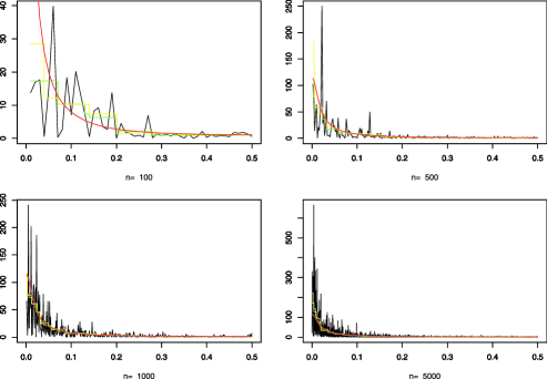
Figure 1: The spectral density (red), the periodogram (black), the estimates $\hat{f}_{n}$ (green) and $\tilde{f}_{n}$ (yellow), for $n=100,500,1\mbox{,}000$ and $5\mbox{,}000$ data points, for Example 1.

$\hat{f},\tilde{f}_{n}$, that are obtained by doing isotonic regression of the data $\{(\lambda_{k},I_{n}(\lambda_{k})),k=1,\ldots,[(n-1)/2]\}$ where $\lambda_{k}=2\pi k/n$. For instance, the discrete version $\hat{f}_{n}^{d}$ of $\hat{f}_{n}$ is calculated as

$$\hat{f}_{n}^{d}=\mathop{\arg\min}_{z\in\mathcal{F}}\sum_{k=1}^{n}\bigl{(}I_{n}(\lambda_{k})-z(\lambda_{k})\bigr{)}^{2}.$$

Note that the limit distribution for $\tilde{f}_{n}$ is stated for the discrete version $\tilde{f}_{n}^{d}$. The simulations were done in R, using the “fracdiff” package. The code is available from the corresponding author upon request.

Example 1.

The first example consists of sums of several AR(1) processes. Let $\{X_{k}\}$ be a stationary AR(1) process, that is, for all $k\in\mathbb{Z}$,

$$X_{k}=aX_{k-1}+\varepsilon_{k},$$

with $|a|<1$. This process has spectral density function $f(\lambda)=(2\pi)^{-1}\sigma^{2}|1-ae^{i\lambda}|^{-2}$ for $-\pi\leq\lambda\leq\pi$, with $\sigma^{2}=\operatorname{var}(\varepsilon_{1}^{2})$ and and thus $f$ is decreasing on $[0,\pi]$. If $X^{(1)},\ldots,X^{(p)}$ are independent AR(1) processes with coefficients $a_{j}$ such that $|a_{j}|<1,j=1,\ldots,p$, and we define the process $X$ by

$$X_{k}=\sum_{j=1}^{p}X_{k}^{(j)},$$

then $X$ has spectral density $f(\lambda)=(2\pi)^{-1}\sum_{j=1}^{p}\sigma_{j}^{2}|1+a_{j}e^{i\lambda}|^{-2}$ which is decreasing on $[0,\pi]$, since it is a sum of decreasing functions. Assuming that we do not know how many AR(1) processes are summed, we have a nonparametric problem: estimate a monotone spectral density. Figure 1 shows a

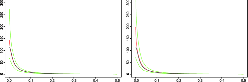
Figure 2: Left plot: spectral density (black), pointwise mean of estimates $\hat{f}_{n}$ (red) and 95% confidence intervals (green). Right plot: spectral density (black), pointwise mean of the estimates $\tilde{f}_{n}$ (red) and 95% confidence intervals (green), for $n=1\mbox{,}000$ data points, for Example 1.

plot of the periodogram, the true spectral density and the nonparametric estimators $\hat{f}_{n}$ and $\tilde{f}_{n}$ for simulated data from a sum of three independent AR(1) processes with $a_{1}=0.5,a_{2}=0.7,a_{3}=0.9$. Figure 2 shows the pointwise means and 95% confidence intervals of $\hat{f}_{n}$ and $\tilde{f}_{n}$ for $1\mbox{,}000$ realizations.

Example 2.

The second example is a sum of an $\operatorname{ARFIMA}(0,d,0)$ process and an AR(1) process. Let $X^{(1)}$ be an $\operatorname{ARFIMA}(0,d,0)$-process with $0<d<1/2$. This has a spectral density $(2\pi)^{-1}\sigma_{1}^{2}|1-e^{i\lambda}|^{-2d}$. If we add an independent AR(1)-process $X^{(2)}$ with coefficient $|a|<1$ the resulting process $X=X^{(1)}+X^{(2)}$ will have spectral density $f(\lambda)=(2\pi)^{-1}\sigma_{1}^{2}|1-e^{i\lambda}|^{-2d}+(2\pi)^{-1}\sigma_{2}^{2}|1-ae^{i\lambda}|^{-2}$ on $[0,\pi]$, and thus the resulting spectral density $f$ will be a monotone function on $[0,\pi]$. As above, if an unknown number of independent processes is added we have a nonparametric estimation problem. Figure 3 shows a plot of the periodogram, the true spectral density and the nonparametric estimators $\hat{f}_{n}$ and $\tilde{f}_{n}$ for simulated time series data from a sum of an $\operatorname{ARFIMA}(0,d,0)$-process with $d=0.2$ and an AR(1)-process with $a=0.5$. Figure 4 shows the pointwise means and 95% confidence intervals of $\hat{f}_{n}$ and $\tilde{f}_{n}$ for $1\mbox{,}000$ realizations.

Table 1 shows mean square root of sum of squares errors (comparing with the true function), calculated on $1\mbox{,}000$ simulated samples of the times series of Example 1. Table 2 shows the analog values for Example 2.

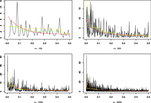
Figure 3: The spectral density (red), the periodogram (black), the estimates $\hat{f}_{n}$ (green) and $\tilde{f}_{n}$ (yellow), for $n=100,500,1\mbox{,}000$ and $5\mbox{,}000$ data points, for Example 2.

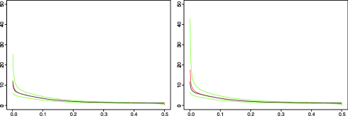
Figure 4: Left plot: spectral density (black), pointwise mean of estimates $\hat{f}_{n}$ (red) and 95% confidence intervals (green). Right plot: spectral density (black), pointwise mean of the estimates $\tilde{f}_{n}$ (red) and 95% confidence intervals (green), for $n=1\mbox{,}000$ data points, for Example 2.

Table 1: MISE values for Example 1

MISE	$\bolds{n=100}$	$\bolds{n=500}$	$\bolds{n=1\mbox{,}000}$	$\bolds{n=5\mbox{,}000}$
$I_{n}$	9.59	$12.96$	$13.67$	$14.25$
$\hat{f}_{n}$	6.38	$5.48$	$4.76$	$2.95$
$\tilde{f}_{n}$	9.11	$8.52$	$7.27$	$4.26$

Table 2: MISE values for Example 2

MISE	$\bolds{n=100}$	$\bolds{n=500}$	$\bolds{n=1\mbox{,}000}$	$\bolds{n=5\mbox{,}000}$
$I_{n}$	$1.80$	$1.99$	$2.02$	$2.07$
$\hat{f}_{n}$	$0.710$	$0.520$	$0.432$	$0.305$
$\tilde{f}_{n}$	$1.12$	$0.803$	$0.659$	$0.472$

Both estimators $\hat{f}_{n}$ and $\tilde{f}_{n}$ seem to have good finite sample properties. As indicated by the theory, $\tilde{f}_{n}$ seems to be less efficient than $\hat{f}_{n}$.

6 Proofs of Theorems 5 and 6

Let $J_{n}$ be the integral of the generic preliminary estimator of the spectral density, that is the integral of $I_{n}$ or of $\log(I_{n})$, let $K$ denote $F$ or the primitive of $\log f$, respectively, and write

$$J_{n}(t)=K(t)+v_{n}(t).$$ (13)

Let $d_{n}\downarrow 0$ be a deterministic sequence, and define the rescaled process and rescaled centering

$$\tilde{v}_{n}(s;t_{0}) = d_{n}^{-2}\{v_{n}(t_{0}+sd_{n})-v_{n}(t_{0})\},$$ (14)

$$g_{n}(s) = d_{n}^{-2}\{K(t_{0}+sd_{n})-K(t_{0})-K^{\prime}(t_{0})d_{n}s\}.$$ (15)

Consider the following conditions:

1. [(AH1)]

2. There exists a stochastic process $\tilde{v}(\cdot;t_{0})$ such that

   $$\tilde{v}_{n}(\cdot;t_{0})\stackrel{{\scriptstyle\mathcal{L}}}{{\rightarrow}}\tilde{v}(\cdot;t_{0}),$$ (16)

   in $D(-\infty,\infty)$, endowed with the topology generated by the supnorm metric on compact intervals, as $n\rightarrow\infty$.

3. For each $\varepsilon,\delta>0$ there is a finite $\tau$ such that

   $$\limsup_{n\rightarrow\infty}P\biggl{(}\sup_{|s|\geq\tau}\biggl{|}\frac{\tilde{v}_{n}(s;t_{0})}{g_{n}(s)}\biggr{|}>\varepsilon\biggr{)} < \delta,$$ (17)

   $$P\biggl{(}\sup_{|s|\geq\tau}\biggl{|}\frac{\tilde{v}(s;t_{0})}{s^{2}}\biggr{|}\varepsilon\biggr{)} < \delta.$$ (18)

4. There is a constant $A<0$ such that for each $c>0$,

   $$\lim_{n\to\infty}\sup_{|s|\leq c}|g_{n}(s)-As^{2}|=0;$$ (19)

5. For each $a\in{\mathbb{R}}$ and $c,\varepsilon>0$

   $$P\bigl{(}\tilde{v}(s;t_{0})(s)-\tilde{v}(0;t_{0})+As^{2}-as\geq\varepsilon|s|\mbox{ for all }s\in[-c,c]\bigr{)}=0.$$ (20)

If there exists a sequence $d_{n}$ such that these four conditions hold, then, defining the process $y$ by $y(s)=\tilde{v}(s;t_{0})+As^{2}$, by Anevski and Hössjer [(2006), Theorems 1 and 2] as $n\rightarrow\infty$, it holds that

$$d_{n}^{-1}\{T(J_{n})^{\prime}(t_{0})-K^{\prime}(t_{0})\}\stackrel{{\scriptstyle\mathcal{L}}}{{\rightarrow}}T(y)^{\prime}(0),$$ (21)

where $T(y)^{\prime}(0)$ denotes the slope at zero of the smallest concave majorant of $y$.

6.1 Proof of Theorem 5

The proof consists in checking conditions (AH1)–(AH4) with $J_{n}=F_{n}$ and $K=F$.

1. [-]

2. It is proved in Lemma 8 below that (16) holds with $d_{n}=n^{1/3}$ and $\tilde{v}(\cdot;t_{0})$ the standard two-sided Brownian motion times $\sqrt{\pi^{2}/6}$.

3. If $f^{\prime}(t_{0})<0$, then (19) holds with $A=\frac{1}{2}f^{\prime}(t_{0})$ and $d_{n}\downarrow 0$ an arbitrary deterministic sequence.

4. Lemma 9 shows that (17) holds and the law of iterated logarithm yields that (18) holds for the two-sided Brownian motion.

5. Finally, (20) also holds for the two-sided Brownian motion.

Thus (21) holds with the process $y$ defined by

$$y(s)=\tfrac 12f^{\prime}(t_{0})s^{2}+\sqrt{2\pi}f(t_{0})W(s).$$

The scaling property of the Brownian motion yields the representation of $T(y)^{\prime}(0)$ in terms of Chernoff’s distribution.

Lemma 8.

Assume the process $\{X_{n}\}$ is given by (10), that (11) holds and that $\mathbb{E}[\varepsilon_{0}^{8}]<\infty$. If $d_{n}=n^{-1/3}$, then the sequence of processes $\tilde{v}_{n}(\cdot;t_{0})$ defined in (14) converges weakly in $C([-c,c])$ to $\sqrt{2\pi}f(t_{0})W$ where $W$ is a standard two-sided Brownian motion.

For clarity, we omit $t_{0}$ in the notation. Write

$$\tilde{v}_{n}(s)=\tilde{v}_{n}^{\varepsilon}(s)+R_{n}(s)$$

with

$$\quad\tilde{v}_{n}^{(\varepsilon)}(s) = d_{n}^{-2}\int_{t_{0}}^{t_{0}+d_{n}s}f(u)\bigl{\{}I_{n}^{(\varepsilon)}(u)-1\bigr{\}}\,{d}u,$$

$$I_{n}^{(\varepsilon)}(u) = \frac{1}{n}\Biggl{|}\sum_{k=1}^{n}\varepsilon_{k}e^{iku}\Biggr{|}^{2},$$

$$R_{n} = d_{n}^{-2}\int_{t_{0}}^{t_{0}+d_{n}s}r_{n}(u)\,{d}u,\qquad r_{n}(u)=I_{n}(u)-f(u)I_{n}^{(\varepsilon)}(u).$$ (23)

Note that $(2\pi)^{-1}I_{n}^{\varepsilon}$ is the periodogram for the white noise sequence $\{\varepsilon_{i}\}$. We first treat the remainder term $R_{n}$. Denote $\mathcal{G}=\{g\dvtx\int_{-\pi}^{\pi}g^{2}(u)f^{2}(u)\,du<\infty\}$. Equation (5.11) (with a typo in the normalization) in Mikosch and Norvaiša (1997) states that if (11) and $\mathbb{E}[\varepsilon_{0}^{8}]<\infty$ hold, then

$$\sqrt{n}\sup_{g\in\mathcal{G}}\int_{-\pi}^{\pi}g(x)r_{n}(x)\,{d}x=o_{P}(1).$$ (24)

Define the set $\tilde{\mathcal{G}}=\{k_{n}(\cdot,s)f\dvtx n\in{\mathbf{N}},s\in[-c,c]\}$. Since $f$ is bounded, we have that $\int k_{n}^{2}(u,s)f^{2}(u)\,{d}u<\infty$, so $\tilde{\mathcal{G}}\subset\mathcal{G}$ and we can apply (24) on $\tilde{\mathcal{G}}$, which shows that $R_{n}$ converges uniformly (over $s\in[-c,c]$) to zero. We next show that

$$\tilde{v}_{n}^{(\varepsilon)}(s)\stackrel{{\scriptstyle\mathcal{L}}}{{\rightarrow}}\sqrt{2\pi}f(t_{0})W(s),$$ (25)

as $n\rightarrow\infty$, on $C({\mathbb{R}})$, where $W$ is a standard two-sided Brownian motion. Since $\{\varepsilon_{k}\}$ is a white noise sequence, we set $t_{0}=0$ without loss of generality. Straightforward algebra yields

$$\tilde{v}_{n}^{(\varepsilon)}(s)=d_{n}^{-2}\{\hat{\gamma}_{n}(0)-1\}F(d_{n}s)+S_{n}(s)$$ (26)

with

$$\hat{\gamma}_{n}(0) = n^{-1}\sum_{j=1}^{n}\varepsilon_{j}^{2},\qquad S_{n}(s)=\sum_{k=2}^{n}C_{k}(s)\varepsilon_{k},$$

$$C_{k}(s) = d_{n}^{3/2}\sum_{j=1}^{k-1}\alpha_{j}(s)\varepsilon_{k-j},\qquad\alpha_{j}(s)=d_{n}^{-1/2}\int_{-d_{n}s}^{d_{n}s}f(u){e}^{iju}\,{d}u.$$

Since $\{\varepsilon_{j}\}$ is a white noise sequence with finite fourth moment, it is easily checked that

$$n\operatorname{var}(\hat{\gamma}_{n}(0)) = \operatorname{var}(\varepsilon_{0}^{2}),$$

$$\sup_{s\in[-c,c]}d_{n}^{-2}\int_{0}^{d_{n}s}f(u)\,{d}u\,|\hat{\gamma}_{n}(0)-1| = O_{P}(d_{n}^{-1}n^{-1/2})=O_{P}\bigl{(}\sqrt{d_{n}}\bigr{)}$$

so that the first term in (26) is negligible. It remains to prove that the sequence of processes $S_{n}$ converges weakly to a standard Brownian motion. We prove the convergence of finite dimension distribution by application of the Martingale central limit theorem [cf., e.g., Hall and Heyde (1980), Corollary 3.1]. It is sufficient to check the following conditions:

$$\lim_{n\to\infty}\sum_{k=2}^{n}\mathbb{E}[C_{k}^{2}(s)] = 2\pi f^{2}(0)s,$$ (28)

$$\lim_{n\to\infty}\sum_{k=2}^{n}\mathbb{E}[C_{k}^{4}(s)] = 0.$$ (29)

By the Parseval–Bessel identity, we have

$$\sum_{j=-\infty}^{\infty}\alpha_{j}^{2}(s)=2\pi d_{n}^{-1}\int_{-d_{n}s}^{d_{n}s}f^{2}(u)\,{d}u\sim 4\pi f^{2}(0)s.$$

Since $\alpha_{0}(s)\sim 2f(0)\sqrt{d_{n}}$, this implies that

$$\sum_{k=2}^{n}\mathbb{E}[C_{k}^{2}(s)]=\sum_{j=1}^{n-1}(1-j/n)\alpha_{j}^{2}(s)\sim\sum_{j=1}^{\infty}\alpha_{j}^{2}(s)\sim 2\pi f^{2}(0)s.$$

This proves condition (28). For the asymptotic negligibility condition (29), we use Rosenthal’s inequality [cf. Hall and Heyde (1980), Theorem 2.12],

$$E[C_{k}^{4}]\leq cstn^{-2}\sum_{j=1}^{k-1}\alpha_{j}^{4}(s)+cstn^{-2}\Biggl{(}\sum_{j=1}^{k-1}\alpha_{j}^{2}(s)\Biggr{)}^{2}=O(n^{-2}),$$

implying $\sum_{k=1}^{n}\mathbb{E}[C_{k}^{4}(s)]=O(n^{-1})$, which proves (29). To prove tightness, we compute the fourth moment of the increments of $S_{n}$. Write

$$S_{n}(s)-S_{n}(s^{\prime})=n^{-1/2}\sum_{k=1}^{n}\sum_{j=1}^{k-1}\alpha_{j}(s,s^{\prime})\varepsilon_{k-j}\varepsilon_{k},$$

with

$$\alpha_{j}(s,s^{\prime})=d_{n}^{-1/2}\int_{d_{n}s^{\prime}}^{d_{n}s}f(u){e}^{iju}\,{d}u+d_{n}^{-1/2}\int_{-d_{n}s}^{-d_{n}s^{\prime}}f(u){e}^{iju}\,{d}u.$$

By Parseval’s inequality, it holds that

$$\sum_{j=1}^{n}\alpha_{j}^{2}(s,s^{\prime})\leq C|s-s^{\prime}|.$$

Applying again Rosenthal’s inequality, we obtain that $\mathbb{E}[|S_{n}(s)-S_{n}(s^{\prime})|^{4}]$ is bounded by a constant times

$$n^{-1}\sum_{j=1}^{n}\alpha_{j}^{4}(s,s^{\prime})+\Biggl{(}\sum_{j=1}^{n}\alpha_{j}^{2}(s,s^{\prime})\Biggr{)}^{2}\leq C|s-s^{\prime}|^{2}.$$

Applying [Billingsley (1968), Theorem 15.6] concludes the proof of tightness.

Lemma 9.

For any $\delta>0$ and any $\kappa>0$, there exists $\tau$ such that

$$\limsup_{n\to\infty}\mathbb{P}\biggl{(}\sup_{|s|\geq\tau}\frac{|\tilde{v}_{n}(s)|}{|s|}>\kappa\biggr{)}\leq\delta.$$ (30)

Without loss of generality, we can assume that $f(t_{0})=1$. Recall that $\tilde{v}_{n}=\tilde{v}_{n}^{(\varepsilon)}+R_{n}$ and $\tilde{v}_{n}^{(\varepsilon)}(s)=F(d_{n}s)\zeta_{n}+S_{n}(s)$, where $\tilde{v}_{n}^{(\varepsilon)}$ and $R_{n}$ are defined in (6.1) and (23), $\zeta_{n}=d_{n}^{-2}(\hat{\gamma}_{n}(0)-1)$ and $S_{n}$ is defined in (26). Then

$$\mathbb{P}\biggl{(}\sup_{s\geq\tau}\frac{|\tilde{v}_{n}(s)|}{s}>\kappa\biggr{)} \leq \mathbb{P}\Bigl{(}\sup_{s\geq\tau}|\zeta_{n}|F(d_{n}s)/s>\kappa/3\Bigr{)}+\mathbb{P}\biggl{(}\sup_{s\geq\tau}\frac{|S_{n}(s)|}{s}>\kappa/3\biggr{)}$$

$${}+\mathbb{P}\biggl{(}\sup_{s\geq\tau}\frac{|R_{n}(s)|}{s}>\kappa/3\biggr{)}.$$

The spectral density is bounded, so $F(d_{n}s)/s\leq Cd_{n}$ for all $s$. Since $\operatorname{var}(\zeta_{n})=O(d_{n}^{-1})$, by (6.1) and the Bienayme–Chebyshev inequality, we get

$$\mathbb{P}\Bigl{(}\sup_{s\geq\tau}|\zeta_{n}|F(d_{n}s)/s>\kappa\Bigr{)}\leq O(d_{n}^{-1}d_{n}^{2})=O(d_{n}).$$

Let $\{s_{j},j\geq 0\}$ be an increasing sequence. Then we have the bound

$$\mathbb{P}\biggl{(}\sup_{s\geq s_{0}}\frac{|S_{n}(s)|}{s}>\kappa\biggr{)} \leq \sum_{j=0}^{\infty}\mathbb{P}\bigl{(}|S_{n}(s_{j})|>\kappa s_{j}\bigr{)}$$

$${}+\sum_{j=1}^{\infty}\mathbb{P}\Bigl{(}{\sup_{s_{j-1}\leq s\leq s_{j}}}|S_{n}(s)-S_{n}(s_{j-1})|>\kappa s_{j-1}\Bigr{)}.$$

From (28), we know that $\operatorname{var}(S_{n}(s))=O(s)$. Thus

$$\sum_{j=0}^{\infty}\mathbb{P}\bigl{(}|S_{n}(s_{j})|>\kappa s_{j}\bigr{)}\leq cst\kappa^{-2}\sum_{j=0}s_{j}^{-1}.$$

Thus if the series $s_{j}^{-1}$ is summable, this sum can be made arbitrarily small by choosing $s_{0}$ large enough. It was shown in the proof of Lemma 8 that

$$\mathbb{E}[|S_{n}(s)-S_{n}(s^{\prime})|^{4}]\leq C|s-s^{\prime}|^{2}.$$

By Billingsley (1968), Theorem 15.6 [or more specifically Ledoux and Talagrand (1991), Theorem 11.1], this implies that

$$\mathbb{P}\Bigl{(}{\sup_{s_{j-1}\leq s\leq s_{j}}}|S_{n}(s)-S_{n}(s_{j-1})|>\kappa s_{j-1}\Bigr{)}\leq\frac{C(s_{j}-s_{j-1})^{2}}{\kappa^{2}s^{2}_{j-1}}.$$

Thus choosing $s_{j}=(s_{0}+j)^{\rho}$ for some $\rho>1$ implies that the series is convergent and

$$\mathbb{P}\biggl{(}\sup_{s\geq s_{0}}\frac{|S_{n}(s)|}{s}>\kappa\biggr{)}=O(s_{0}^{-1}),$$

which is arbitrarily small for large $s_{0}$.

To deal with the remainder term $R_{n}$, we prove that $\mathbb{P}({\sup_{s\geq s_{0}}}|R_{n}(s)|/s>s_{0})=o_{P}(1)$ by the same method as that used for $S_{n}$. Thus we only need to obtain a suitable bound for the increments of $R_{n}$. By definition of $R_{n}$, we have, for $s<s^{\prime}$,

$$R_{n}(s^{\prime})-R_{n}(s)=d_{n}^{-2}\int_{t_{0}+d_{n}s}^{t_{0}+d_{n}s^{\prime}}f(u)r_{n}(u)\,{d}u.$$

Since $f$ is bounded, by Hölder’s inequality, we get

$$\mathbb{E}[|R_{n}(s^{\prime})-R_{n}(s)|^{2}]\leq\|f\|_{\infty}n(s^{\prime}-s)\int_{t_{0}+d_{n}s}^{t_{0}+d_{n}s^{\prime}}\mathbb{E}[r_{n}^{2}(u)]\,{d}u.$$

Under (11), it is known [see, e.g., Brockwell and Davis (1991), Theorem 10.3.1] that

$$\mathbb{E}[r_{n}^{2}(u)]\leq Cn^{-1}.$$

Hence,

$$\mathbb{E}[|R_{n}(s^{\prime})-R_{n}(s)|^{2}]\leq Cd_{n}n(s^{\prime}-s)^{2}.$$

The rest of the proof is similar to the proof for $S_{n}$. This concludes the proof of (30).

6.2 Sketch of proof of Theorem 6

The proof consists in checking conditions (AH1)–(AH4) with $J_{n}$ and $K_{n}$ now defined by $J_{n}(t)=\int_{0}^{t}\{\log I_{n}(s)+\gamma\}\,{d}s$ and $K(t)=\int_{0}^{t}\log f(2\pi[ns/2\pi]/n)\,{d}s$. Let $\lambda_{k}=2k\pi/n$ denote the so-called Fourier frequencies. For $t\in[0,\pi]$, denote $k_{n}(t)=[nt/2\pi]$. Denote

$$\xi_{k}=\log\{I_{n}(\lambda_{k})/f(\lambda_{k})\}+\gamma,$$

where $\gamma$ is Euler’s constant. Then

$$v_{n}(t)=J_{n}(t)-K(t)=\frac{2\pi}{n}\sum_{j=1}^{k_{n}(t)}\xi_{j}+\bigl{(}t-\lambda_{k_{n}(t)}\bigr{)}\xi_{k_{n}(t)}.$$

The log-periodogram ordinates $\xi_{j}$ are not independent, but sums of log-periodogram ordinates, such as the one above, behave asymptotically as sums of independent random variables with zero mean and variance $\pi^{2}/6$ [cf. Soulier (2001)], and bounded moments of all order. Thus, for $t_{0}\in(0,\pi)$, the process $\tilde{v}_{n}(s;t_{0})=d_{n}^{-2}\{v_{n}(t_{0}+d_{n}s)-v_{n}(t_{0})\}$ with $d_{n}=n^{-1/3}$ converges weakly in $D(-\infty,\infty)$ to the two-sided Brownian motion with variance $2\pi^{4}/3$. It can be shown by using the moment bounds of Soulier (2001) that (17) holds. Finally, if $f$ is differentiable at $t_{0}$, it is easily seen that $d_{n}^{-2}(K(t_{0}+d_{n}s)-K(t_{0})-d_{n}sJ^{\prime}_{b}(t_{0})\}$ converges to $\frac{1}{2}As^{2}$ with $A=f^{\prime}(t_{0})/f(t_{0})$.

References

- Anevski and Hössjer (2006) Anevski, D. and Hössjer, O. (2006). A general asymptotic scheme for inference under order restrictions. Ann. Statist. 34 1874–1930. \MR2283721
- Billingsley (1968) Billingsley, P. (1968). Convergence of Probability Measures. Wiley, New York. \MR0233396
- Brockwell and Davis (1991) Brockwell, P. J. and Davis, R. A. (1991). Time Series: Theory and Methods. Springer, New York. \MR1093459
- Dahlhaus (1989) Dahlhaus, R. (1989). Efficient parameter estimation for self-similar processes. Ann. Statist. 17 1749–1766. \MR1026311
- Davies and Kovac (2004) Davies, P. L. and Kovac, A. (2004). Densities, spectral densities and modality. Ann. Statist. 32 1093–1136. \MR2065199
- Dzhaparidze (1986) Dzhaparidze, K. (1986). Parameter Estimation and Hypothesis Testing in Spectral Analysis of Stationary Time Series. Springer, New York. \MR0812272
- Gill and Levit (1995) Gill, R. D. and Levit, B. Y. (1995). Applications of the Van Trees inequality: A Bayesian Cramér–Rao bound. Bernoulli 1 59–79. \MR1354456
- Groeneboom and Wellner (2001) Groeneboom, P. and Wellner, J. A. (2001). Computing Chernoff’s distribution. J. Comput. Graph. Statist. 10 388–400. \MR1939706
- Hall and Heyde (1980) Hall, P. and Heyde, C. C. (1980). Martingale Limit Theory and its Application. Academic Press, New York. \MR0624435
- Holden (1976) Holden, A. V. (1976). Models of the Stochastic Activity of Neurons. Springer, Berlin. \MR0449766
- Hörmander (2007) Hörmander, L. (2007). Notions of Convexity. Birkhäuser, Boston. \MR2311920
- Hurvich, Deo and Brodsky (1998) Hurvich, C. M., Deo, R. and Brodsky, J. (1998). The mean squared error of Geweke and Porter-Hudak’s estimator of the memory parameter of a long-memory time series. J. Time Ser. Anal. 19 19–46. \MR1624096
- Kerner and Harris (1994) Kerner, C. and Harris, P. E. (1994). Scattering attenuation in sediments modeled by ARMA processes—validation of simple Q modeles. Geophysics 53 1813–1826.
- Ledoux and Talagrand (1991) Ledoux, M. and Talagrand, M. (1991). Probability in Banach Spaces. Isoperimetry and Processes. Springer, Berlin. \MR1102015
- Mammen (1991) Mammen, E. (1991). Estimating a smooth monotone regression function. Ann. Statist. 19 724–740. \MR1105841
- McCoy, Walden and Percival (1998) McCoy, E. J., Walden, A. T. and Percival, D. B. (1998). Multitaper spectral estimation of power law processes. IEEE Trans. Signal Process. 46 655–668. \MR1718617
- McHardy and Czerny (1987) McHardy, I. and Czerny, B. (1987). Fractal X-ray time variablity and spectral invariance of the Seyfert galaxy NGC 5507. Nature 325 696–698.
- Mikosch and Norvaiša (1997) Mikosch, T. and Norvaiša, R. (1997). Uniform convergence of the empirical spectral distribution function. Stochastic Process. Appl. 70 85–114. \MR1472960
- Moulines and Soulier (1999) Moulines, E. and Soulier, P. (1999). Broadband log-periodogram regression of time series with long-range dependence. Ann. Statist. 27 1415–1439. \MR1740105
- Munk and Macdonald (2009) Munk, W. H. and Macdonald, G. J. F. (2009). The Rotation of the Earth, A Geophysical Discussion. Cambridge Univ. Press, Cambridge.
- Percival (1991) Percival, D. B. (1991). Characterization of frequency stability: Frequence-domain estimation of stability measures. IEEE Process. 79 961–972.
- Percival and Walden (1993) Percival, D. B. and Walden, A. T. (1993). Spectral Analysis for Physical Applications. Cambridge Univ. Press, Cambridge. \MR1297763
- Prakasa Rao (1969) Prakasa Rao, B. L. S. P. (1969). Estimation of a unimodal density. Sankhyā Ser. A 31 23–36. \MR0267677
- Robertson, Wright and Dykstra (1988) Robertson, T., Wright, F. T. and Dykstra, R. L. (1988). Order Restricted Statistical Inference. Wiley, Chichester. \MR0961262
- Robinson (1995) Robinson, P. M. (1995). Log-periodogram regression of time series with long range dependence. Ann. Statist. 23 1048–1072. \MR1345214
- Soulier (2001) Soulier, P. (2001). Moment bounds and central limit theorem for functions of Gaussian vectors. Statist. Probab. Lett. 54 193–203. \MR1858634
- Wright (1981) Wright, F. T. (1981). The asymptotic behavior of monotone regression estimates. Ann. Statist. 9 443–448. \MR0606630