Extreme events in discrete nonlinear lattices

Abstract

We perform statistical analysis on discrete nonlinear waves generated though modulational instability in the context of the Salerno model that interpolates between the intergable Ablowitz-Ladik (AL) equation and the nonintegrable discrete nonlinear Schrödinger (DNLS) equation. We focus on extreme events in the form of discrete rogue or freak waves that may arise as a result of rapid coalescence of discrete breathers or other nonlinear interaction processes. We find power law dependence in the wave amplitude distribution accompanied by an enhanced probability for freak events close to the integrable limit of the equation. A characteristic peak in the extreme event probability appears that is attributed to the onset of interaction of the discrete solitons of the AL equation and the accompanied transition from the local to the global stochasticity monitored through the positive Lyapunov exponent of a nonlinear map.

Introduction.- The motivation of the present work stems from observations of the sudden appearance of extremely large amplitude sea waves referred to as rogue or freak waves Kharif . These waves appear very suddenly in relatively calm seas, reach amplitudes of over $20m$ and may destroy or sink small as well as large vessels Muller . Theoretical analysis of ocean freak waves has been linked to nonlinearities in the waver wave equations, studied though the nonlinear Schrödinger (NLS) equation and shown that the probability of their appearance is not insignificant Onorato . A scenario for freak wave generation in NLS is through a Benjamin-Feir (modulational) instability, resulting in self-focusing effects and subsequent formation of freak waves Zakharov . Modulational instability (MI) induces local exponential growth in the wave train amplitude Onorato1 ; Shukla that has been confirmed experimentally and numerically Ruban .

Intriguingly, there are completely different physical systems that possess the required nonlinear characteristics which favour the appearance of rogue waves. Recent observation of optical rogue waves in a microstructured optical fiber was reported Solli in a regime near the threshold of soliton-fission supercontinuum generation, i.e., in a region where MI plays a key role in the dynamics. A generalized NLS equation was used successfully to model the generation of optical rogue waves while, additionally, control and manipulation of rogue soliton formation was also discussed Dudley . The mechanism of the rogue waves creation, or, more generally of extreme events, has become an issue of principal interest in various other contexts as well, since rogue waves can signal catastrophic phenomena such as an earthquake, a thunderstorm, or a severe financial crisis. Knowledge of the probability of occurrence of extreme events and the capability to predict the time at which such an event may take place is of a great value. Such events are usually rare, and they exhibit ”extreme-value” statistics, typically characterized by heavy-tailed probability distributions. Experimental observation of optical rogue-wave-like fluctuations in fiber Raman amplifiers show that the probability distribution of their peak power follows a power law Hammani .

In this work we focus on the discrete counterparts of rogue waves that may appear in nonlinear lattices as a result of discrete soliton or breather induction and their mutual interactions. Specifically we investigate the role of integrability in the formation of discrete rogue waves (DRW) and the resulting extreme event statistics. Their appearance may affect dramatically the physical systems. We use the Salerno model Salerno that through a unique parameter interpolates between a fully integrable discrete lattice, viz. the Ablowitz-Ladik (AL) lattice Ablowitz , and the nonintegrable DNLS equation ELS ; MT . One of the basic questions to be addressed below is the probability of occurrence of a DRW as a function of the degree of integrability of the lattice and thus study the role of the latter in the production of extreme lattice events Nicolis .

The Salerno model.- The Salerno model (SM) is given through the following set of equations

$$i\frac{d\psi_{n}}{dt}=-(1+\mu|\psi_{n}|^{2})(\psi_{n+1}+\psi_{n-1})-\gamma|\psi_{n}|^{2}\psi_{n}$$ (1)

where $\mu$ and $\gamma$ are two nonlinearity parameters. When $\mu=0$ the model becomes the DNLS equation while for $\gamma=0$ it reduces to AL. Several properties of the model such as integrability Rumpf and stability of localized travelling waves Cai ; Hennig have been analyzed. Both the norm $N$ and the Hamiltonian $H$ of the model are conserved quantities. They are given by

$$N = \frac{1}{\mu}\sum_{n}\ln{|1+\mu|\psi_{n}|^{2}|},$$ (2)

$$H = \sum_{n}\left[\frac{\gamma}{\mu^{2}}\ln|1+\mu|\psi_{n}|^{2}|-\frac{\gamma}{\mu}|\psi_{n}|^{2}-2Re[\psi_{n}\psi_{n+1}^{*}]\right].$$ (3)

It is also known that Eq. (1) exhibits MI, which may give rise to stationary, spatially localized solutions in the form of discrete breathers (DBs), i.e., periodic and spatially localized nonlinear excitations DBs . The MI induced DBs appear in random lattice locations and may be mobile. High-amplitude DBs tend to absorb low-amplitude ones, resulting after some time in a small number of very high amplitude excitations, which may get pinned at a specific lattice site due to the Peierls-Nabarro potential barrier in nonintegrable lattices Kivshar1 . In general, high-amplitude DBs are virtual bottlenecks which slow down the relaxation processes in nonlinear lattices Tsironis ; Rasm , and it has been proposed that they may serve as models for freak waves Dysthe . The development of MI in Eq. (1) can be analyzed with the linear stability analysis of its the plane wave solutions perturbed by small phase and amplitude perturbations Maluckov . The interplay between the on-site and intersite nonlinear terms (i.e., according to the variation of their relative strength through $\mu$ and $\gamma$), may change MI properties and, consequently, the conditions for the DBs to exist in the lattice Kivshar . The SM has recently found applications in modelling Bose-Einstein condensates of dipolar atoms in a strong periodic potential Gomez , dilute Bose-Einstein condensates trapped in a periodic potential Trombettoni , and even biological systems Salerno1 .

For later convenience in the numerical simulation, the variables $\psi_{n}$ in Eq. (1) are rescaled as $\psi_{n}=\xi_{n}/\sqrt{\mu}$, so that in terms of $\xi_{n}$ the dynamic equations read

$$i\frac{d\xi_{n}(t)}{dt}=-(1+|\xi_{n}(t)|^{2})(\xi_{n+1}+\xi_{n-1})-\Gamma|\xi_{n}(t)|^{2}\xi_{n},$$ (4)

where $\Gamma=\gamma/\mu$. Therefore, the whole two-dimensional parameter space $(\gamma,\mu)$ can be scaled by $\mu=1$, leaving $\gamma$ as a free parameter. With that scaling we may go as close to the DNLS limit as we want to, by simply let $\Gamma$ to attain very large values. However, the exact DNLS limit $\mu=0$ has to be calculated separately.

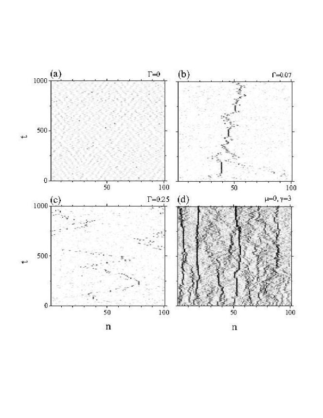
Figure 1: Evolution of the scaled amplitudes $|\xi_{n}|$ for a lattice of size $N=101$, with $\Gamma$ ($\mu$ and $\gamma$ in the DNLS case), is shown on the figure. The initial conditions for all cases are $\xi_{n}=1$ for any $n$ (uniform) plus a small amount of white noise.

Statistics of extreme events.- We integrate numerically the system of Eqs. (4) with periodic boundary conditions using a sixth order Runge-Kutta algorithm with fixed time-stepping $\Delta t=10^{-4}$. We started simulations with different initial conditions (the plane wave, uniform background with white noise and Gaussian noise) which gave similar results. Here we present calculations in which the initial condition is uniform, $\xi_{n}=1$ for any $n$, with the addition of a small amount of white noise to accelerate the development of the MI. The uniform solution is chosen in the interval where it is known from linear stability analysis that it is unstable. By varying the nonlinearity parameters we identify broadly three regimes of DRWs that are shown as spatiotemporal evolutions in Fig. 1. For the purely integrable AL lattice ($\Gamma=0$) DBs are mobile and essentially noninteracting; as a result we do not observe significant formation of high DRWs (Fig. 1a). In the vicinity of the AL limit, i.e. for small $\Gamma$ ($\Gamma\sim 0.1$), there is an onset of weak interaction of the localized modes of the AL lattice leading to a significant increase in DRW formation that are mobile (Fig. 1b,c). In this regime the DBs are highly mobile indicating that DB merging could be responsible for creation of high-amplitude localized waves. For $\Gamma>>0.1$ on the other hand, DNLS-type behavior dominates the SM and localized structures that are initially created through the MI become easily trapped in the lattice (Fig. 1d).

The three regimes mentioned previously are probed by calculating the time-averaged height distributions $P_{h}$. We first define the forward (backward) height at the $n-$th site as the difference between two successive minimum (maximum) and maximum (minimum) values of $|\xi_{n}(t)|$. We use then both the forward and the backward heights for the calculation of the local height distribution; after spatial averaging the latter results in the height probability densities (HPDs) shown in Fig. 2. We note that the tails of the HPDs are related to extreme events and the appearance of DRWs. For $\Gamma$ finite the HPDs are sharply peaked but have extended tails indicating that extreme events are more than several times as large as the mean distribution height. In the DNLS limit ($\Gamma\gg 1$) the obtained HPD is very close to the Rayleigh distribution whose tails decay very fast VanKampen , indicating negligible probability for the occurrence of extreme events (dotted curve in Fig. 2). In all the other cases the decay of the tails of the HPDs is much slower.

In order to probe further the onset of extreme discrete events we employ the practice used in water waves and define a DRW as one that has a height greater than $h_{th}=2.2h_{s}$, with $h_{s}$ being the significant wave height. The latter is defined as the average height of the one-third higher waves in the height distribution. As a result, the probability of occurrence of extreme DRW events $P_{ee}=P_{h}(h>h_{th})$ is obtained by integration of the (normalized) HPD from $h=h_{th}$ up to infinity. By evaluating several HPDs as those in Fig. 2 we may estimate the probability of occurrence of DRWs $P_{ee}$ as a function of the parameter $\Gamma$ (the results are shown in Fig. 3). We note that the probability for the occurrence of a DRW has a certain value in the AL case, subsequently peaks for small values of $\Gamma$ and decays precipitously when $\Gamma>>1$. This behavior of the probability $P_{ee}$ is compatible with the DB picture outlined earlier, viz. in the very weakly nonintegrable regime the AL modes may interact leading to DB fusion and DRW generation. On the other hand, as nonintegrability becomes stronger, the scattering of the AL modes is more chaotic leading to a suppression of DRW formation.

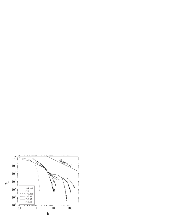
Figure 2: The normalized height probability density $P_{h}(h)$ for several values of $\Gamma$ and for the DNLS limit (with $\gamma=6$). The line with slope $-1$ is added to assist comparisons and corresponds to $P_{h}\sim 1/h$. Approximately vertical drop corresponds to the DNLS limit with an exponential tail. The increase of $\Gamma(\mu=1)$ leads to the decrease of the slope and appearance of plateau on the $P_{h}$ curve; the latter increases the extreme event probability leading a maximum at $\Gamma=0.07$ (Fig. 3.)

Figure 3: The normalized probability $P_{ee}=P_{h}(h\geq h_{th})$ for the occurrence of extreme events as a function of the integrability parameter $\Gamma$. All data present averaged results of five numerical measurements differing in the initial conditions.

Map approach.- In order to probe deeper on the formation of DRWs we substitute $\psi_{n}=\phi_{n}\exp(-i\omega t)$ into Eq. (1), with $\phi_{n}$ a real-valued function of the lattice site $n$, and obtain the stationary equation

$$\omega\phi_{n}+(1+\mu|\phi_{n}|^{2})(\phi_{n+1}+\phi_{n-1})+\gamma|\phi_{n}|^{2}\phi_{n}=0,$$ (5)

which can be transformed in the two-dimensional map

$$x_{n+1}=-\frac{\omega+\gamma x_{n}^{2}}{1+\mu x_{n}^{2}}x_{n}-y_{n},\qquad y_{n+1}=x_{n},$$ (6)

where we have defined $x_{n}=\phi_{n}$ and $y_{n}=\phi_{n-1}$. Eqs. (6) represent a real analytic area-preserving map Hennig ; Hennig1 with the lattice index $n$ playing the role of discrete ’time’.

The phase portraits of the map Eq. (6) for several $\Gamma$-values are shown in Fig. 4. In the AL limit, the phase space consists of perfectly disconnected separatrices while for non-zero $\Gamma$, the stable and unstable manifolds intersect transversely, resulting in the generation of a homoclinic tangle. With increasing $\Gamma$ the motion near separatrices becomes exceedingly complicated and the trajectories wander irregularly before approaching an attracting set (Figs. 4b and 4c). Moreover, for any $\Gamma\neq 0$, the position of separatrices in phase space changes in time, resulting in overlapping of neighboring separatrices and diffusion in those regions which have been traversed by a separatrix. The sharp peak of the probability of occurrence of extreme events $P_{ee}(h>h_{th})$ in the SM (Fig. 3) can be associated with the opening of a stochasticity web, when orbits fast explore all extended narrow stochasticity regions leading to an anomalous relaxation phase Rumpf ; VanKampen . This event signs the transition from the local to global stochasticity Lichtenberg in SM. On the other hand, the decrease of $P_{ee}(h>h_{th})$ for larger $\Gamma$’s is related to the increasingly longer trapping time in more developed stochasticity region.

The Melnikov analysis in the SM Hennig shows that the magnitude of the separatrix splitting and the consequent development of stochasticity depends on the $\Gamma/|\omega|$ ratio. The conjecture that $P_{ee}$ is associated with the complexity of the phase portraits of the corresponding maps implies that $P_{ee}$ should also depend on the $\Gamma/|\omega|$ ratio. In our case $|\omega|$ is related to the modulation frequency of the initially uniform solution $U$ with the relation $|\omega|=(\gamma+2\mu)U^{2}+2$, which, through the MI process it transformed into a train of localized DB-like configurations. We have checked numerically that for fixed ratio $\Gamma/|\omega|$ and different values of $U$ and $\Gamma$ we obtain the same HPD. As a consequence, the probability of extreme events $P_{ee}$ as a function of the $\Gamma/|\omega|$ is qualitatively the same with that of $P_{ee}$ as a function of $\Gamma$ shown in Fig. 3.

The degree of nonintegrability in the SM model can be quantified by calculating the Lyapunov exponents of the corresponding maps Maluckov1 . We have thus calculated the maximum Lyapunov exponent $L$ Lichtenberg for the map Eq. (6), for the parameters used in the calculation of the phase portrait shown in the left panels of Fig. 4. It is observed that homoclinic orbits which correspond to perfect separatrices are characterized by vanishing Lyapunov exponent (Fig. 4a). With increasing stochasticity, $L$ tends to a finite positive value which generally depends on the values of the parameters and the initial conditions (Figs. 4a and 4b).

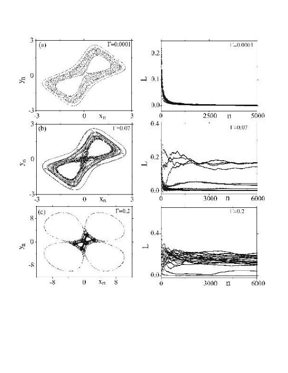
Figure 4: Orbits started at different initial positions in the neighborhood of map origin and corresponding the one-dimensional Liapunov exponents.

Conclusions.- The probability of occurrence of extreme events $P_{ee}$ in the SM results from the competition between the self-focusing and the energy transport mechanisms which are implicitly correlated with the degree of integrability of the model Rumpf . Through modulational instability and starting from a slightly perturbed uniform background we can generate high-amplitude localized moving structures of the DB type that lead to the formation of extreme events of DRW type. Depending on their number, amplitude and life-time, they may prevent of facilitate the energy flow in the lattice, affecting thus the probability of extreme event formation $P_{ee}$. We find that the latter probability depends strongly on $\Gamma$ that affects the degree of integrability of the lattice: DRW are much more probable very close to the integrable SM limit rather than in the nonintegrable one. We find a resonance-like maximum in $P_{ee}(\Gamma)$ that, through a nonlinear map approach, is linked to separatrix breaking and the onset of global stochasticity. This regime corresponds physically to weak interaction between the quasi-integrable modes of the system.

A. M. and Lj.H. acknowledge support from the Ministry of Science of Serbia (Project 141034). One of us (GPT) acknowledges discussions with Oriol Bohigas.

References

- (1) C. Kharif and E. Pelinovsky, Eur. J. Mech. B Fluids 22, 603 (2003).
- (2) P. Müller, C. Garrett, and A. Osborne, Oceanography 18, 66 (2005).
- (3) M. Onorato, A. R. Osborne, M. Serio, and S. Bertone, Phys. Rev. Lett. 86, 5831 (2001).
- (4) V. E. Zakharov, A. I. Dyachenko, and A. O. Prokofiev, Eur. J. Mech. B Fluids 25, 677 (2006).
- (5) M. Onorato, A. R. Osborne, and M. Serio, Phys. Rev. Lett. 96, 014503 (2006).
- (6) P. K. Shukla, I. Kourakis, B. Eliasson, M. Marklund, and L. Stenflo, Phys. Rev. Lett. 97, 094501 (2006).
- (7) V. P. Ruban, Phys. Rev. Lett. 99, 044502 (2007).
- (8) D. R. Solli, C. Ropers, P. Koonath, and B. Jalali, Nature 450, 1054 (2007).
- (9) J. M. Dudley, G. Genty, and B. J. Eggleton, Opt. Express 16, 3644 (2008).
- (10) K. Hammani, C. Finot, J. M. Dudley, and G. Millot, Opt. Express 16, 16467 (2008).
- (11) M. Salerno, Phys. Rev. A 46, 6856 (1992).
- (12) M. J. Ablowitz and J. F. Ladik, J. Math. Phys. 17, 1011 (1976).
- (13) C. H. Eilbeck, P. S. Lomdahl, and A. C. Scott, Physica D 16, 318 (1985).
- (14) M. Molina and G. P. Tsironis, Physica D, 65, 267 (1993).
- (15) C. Nicolis, V. Balakrishnan, and G. Nicolis, Phys. Rev. Lett. 97, 210602 (2006).
- (16) B. Rumpf and A. C. Newell, Physica D 184, 162 (2003).
- (17) D. Cai, A. R. Bishop, and N. Grønbech-Jensen, Phys. Rev. Lett. 72, 591 (1994).
- (18) D. Hennig , K. Ø. Rasmussen, H. Gabriel and A. Bülow, Phys. Rev. E 54, 5788 (1996); D. Hennig, N. G. Sun, H. Gabriel and G. P. Tsironis, Phys. Rev. E 52, 255 (1995).
- (19) S. Flach and C. R. Willis, Phys. Rep. 295, 181 (1998); S. Flach and A. V. Gorbach, Phys. Rep. 467, 1 (2008); and references therein.
- (20) Yu. S. Kivshar and D. K. Campbell, Phys. Rev. E 48, 3077 (1993).
- (21) G. P. Tsironis and S. Aubry, Phys. Rev. Lett. 77, 5225 (1996).
- (22) K. Ø. Rasmussen, S. Aubry, A. R. Bishop and G. P. Tsironis, Eur. Jour. Phys. B 15, 169 (2000).
- (23) K. B. Dysthe and K. Trulsen, Physica Scripta T82, 48 (1999).
- (24) A. Maluckov, Lj. Hadžievski, and B. Malomed, Phys. Rev. E 76, 046605 (2007).
- (25) Yu. S. Kivshar and M. Salerno, Phys. Rev. E 49, 3543 (1994).
- (26) J. Gomez-Gardees, B. A. Malomed, L. M. Floria, and A. R. Bishop, Phys. Rev. E 73, 036608 (2006).
- (27) A. Trombettoni and A. Smerzi, Phys. Rev. Lett. 86, 2353 (2001).
- (28) M. Salerno, Phys. Rev. A 44, 5292 (2001).
- (29) N. G. Van-Kampen, Stochastic Processes in Physics and Chemistry (North-Holland, Amsterdam) (1981).
- (30) D. Hennig and G. P. Tsironis, Phys. Rep. 307, 333 (1999).
- (31) A. J. Lichtenberg and M. A. Lieberman, Regular and Chaotic Dynamics (Springer-Verlag, New York, Inc.) (1992).
- (32) A. Maluckov, Lj. Hadžievski, and M. Stepić, Physica D 216, 95 (2006).