Diverse routes to oscillation death in a coupled oscillator system

Abstract

We study oscillation death (OD) in a well-known coupled-oscillator system that has been used to model cardiovascular phenomena. We derive exact analytic conditions that allow the prediction of OD through the two known bifurcation routes, in the same model, and for different numbers of coupled oscillators. Our exact analytic results enable us to generalize OD as a multiparameter-sensitive phenomenon. It can be induced, not only by changes in couplings, but also by changes in the oscillator frequencies or amplitudes. We observe synchronization transitions as a function of coupling and confirm the robustness of the phenomena in the presence of noise. Numerical and analogue simulations are in good agreement with the theory.

Oscillations, chaos, and bifurcations Synchronization; coupled oscillators Nonlinear dynamics and chaos

Coupled oscillator systems exhibit a variety of phenomena relevant to physics, biology, and other branches of science and technology. Here, we study oscillation death (OD) [1], a form of synchronization [2] in which the oscillators interact in such a way as to quench each other’s oscillations [3, 4, 5, 6]. This intriguing phenomenon was noted in the 19th century by Rayleigh [2], who found that adjacent organ pipes of the same pitch can reduce each other to silence. Since then, OD has been studied in diverse applications including oceanography [7], chemical engineering [8], solid-state lasers [9] and a variety of other experimental systems [4, 10, 11, 12]. OD is known to occur via two distinct bifurcation mechanisms: (i) Hopf bifurcation, where the coupling induces stability at the origin of the phase space, thus collapsing the orbits to zero, which can happen only if the oscillators are sufficiently different [5, 13, 14, 15, 16] (or for identical oscillators if there are delays [17, 18] in the coupling); or (ii) for non-identical oscillators, saddle-node bifurcation [4] in which new fixed points appear on/near the coupled limit cycles, annihilating the periodic orbits. Recently, Karnatak et al. [19] were able to produce OD in two identical coupled oscillators through the saddle-node route, using dissimilar non-delayed coupling.

In this Letter, we show that a coupled-oscillator system, which has been used extensively in modeling coupled rhythmic processes in mathematics, physics and biology [27] can undergo OD via both bifurcation routes. We obtain exact analytic conditions for OD, and compare the theory with numerical simulations and analogue electronic experiments. We thus generalize OD as a phenomenon that occurs, not only through coupling-increased dissipativity [2], but also when a measure of dispersion among the parameters of the coupled system is exceeded [21]. We also show that, near the onset of death, the coupled system alternates between periodic, quasiperiodic and even chaotic behavior, reflecting the complex temporal variability observed in real biological systems [22, 23].

Our model is a set of five coupled oscillators that successfully reproduces many phenomena seen in the cardiovascular system (CVS), e.g. modulation [20] and synchronization [24]. Each oscillator has its own characteristic frequency and amplitude [25] (see Table 1) and emulates a particular physiological function. Heart and respiration are obvious physiological processes; the myogenic oscillation is related to the intrinsic self-regulatory activity of the smooth muscle tissue in the walls of the blood vessels; the neurogenic oscillation is associated with the neural control by the central nervous system; and the nitric oxide related endothelial oscillation is associated with metabolic activity mediated by the endothelial tissue that lines the whole CVS [26].

The basic unit,

$$\begin{array}[]{c c l}\dot{x}_{i}&=&-x_{i}q_{i}-y_{i}\omega_{i}+P_{i}(\textbf{X},\mathbf{Y})\\ \dot{y}_{i}&=&-y_{i}q_{i}+x_{i}\omega_{i}+Q_{i}(\textbf{X},\mathbf{Y}),\end{array}$$ (1)

is the Poincaré oscillator [27] with: $i=1,\ldots,m$, $(m=5)$; $q_{i}=\alpha\left(\sqrt{(x_{i}^{2}+y_{i}^{2})}-a_{i}\right)$; $a_{i}$, $\omega_{i}=2\pi f_{i}$ and $\alpha$ are constants that represent amplitude, frequency and dissipation rate respectively. X and Y $\in R^{m}$, and $P_{i},Q_{i}:R^{m}\rightarrow R$ are scalar coupling functions. We suppose that the inter-oscillator interactions can be approximated by a mean field, so that $P_{i}(\mathbf{X},\mathbf{Y})=\frac{1}{m}\displaystyle\sum{x_{j}}$, and $Q_{i}(\mathbf{X},\mathbf{Y})=0$.

Table 1: Typical values of frequency (Hz) and relative amplitude (arbitrary units) of physiological rhythms in humans, as measured in blood flow by laser-Doppler flowmetry and analysed by wavelet transform. The characteristic frequencies vary around the values indicated; the amplitudes are only estimated based on measurements [20, 25].

Activity	Frequency	Amplitude
Heart	1.1 Hz	0.5 a.u.
Respiration	0.3 Hz	1.0 a.u.
Myogenic	0.1 Hz	1.0 a.u.
Neurogenic	0.04 Hz	1.0 a.u.
Endothelial	0.01 Hz	0.5 a.u.

We now review briefly some basic concepts, assuming an autonomous $n$–dimensional dynamical system:

$$\begin{array}[]{c c l}\dot{\textbf{Z}}&=&\textbf{F}(\textbf{Z}),\end{array}$$ (2)

where $\textbf{Z}\in R^{n}$ and $\textbf{F}:R^{n}\rightarrow R^{n}$ is a general nonlinear vector function. All the points, $\textbf{Z}^{*}$, in phase space satisfying the equation $\textbf{F}(\textbf{Z}^{*})=\textbf{0}$, are called fixed points of the dynamical system (2). Their stability and quality can be determined by the eigenvalues of the Jacobi matrix, provided their real parts are nonzero:

$$\det\left\{\frac{\partial\textbf{F}(\textbf{Z})}{\partial\textbf{Z}}|_{\textbf{Z}=\textbf{Z}^{*}}-\lambda\textbf{I}\right\}=0$$ (3)

We consider first the case of two coupled oscillators, modelling e.g. the cardio-respiratory interactions,

$$\begin{array}[]{c c l}\dot{x_{1}}&=&-x_{1}\alpha(\sqrt{x_{1}^{2}+y_{1}^{2}}-a_{1})-y_{1}\omega_{1}+\epsilon(x_{1}+x_{2}),\\ \dot{y_{1}}&=&-y_{1}\alpha(\sqrt{x_{1}^{2}+y_{1}^{2}}-a_{1})+x_{1}\omega_{1},\\ \dot{x_{2}}&=&-x_{2}\alpha(\sqrt{x_{2}^{2}+y_{2}^{2}}-a_{2})-y_{2}\omega_{2}+\epsilon(x_{1}+x_{2}),\\ \dot{y_{2}}&=&-y_{2}\alpha(\sqrt{x_{2}^{2}+y_{2}^{2}}-a_{2})+x_{2}\omega_{2}.\end{array}$$ (4)

Here the origin is always a fixed point. For $\epsilon=0$, this point is unstable (focus or node). Besides this fixed point, there is a stable limit cycle, corresponding to autonomous oscillations. Eq. (3) for the point $\textbf{Z}^{*}=\textbf{0}$ and $\epsilon\neq 0$ in the dynamical system  (4) will be:

$$\left|\begin{array}[]{c c c c}(\alpha a_{1}+\epsilon)-\lambda&-\omega_{1}&\epsilon&0\\ \omega_{1}&\alpha a_{1}-\lambda&0&0\\ \epsilon&0&(\alpha a_{2}+\epsilon)-\lambda&-\omega_{2}\\ 0&0&\omega_{2}&\alpha a_{2}-\lambda\end{array}\right|=0.$$ (5)

From (5) we determine that the origin can become a stable fixed point if

$$\begin{array}[]{c}2\alpha a_{1}+\epsilon<0,\\ 2\alpha a_{2}+\epsilon<0,\end{array}$$ (6)

in which case the limit cycle no longer exists. Thus, if $a_{2}>a_{1}$, then $\epsilon<-2\alpha a_{2}$ is a sufficient condition for OD. This is the Hopf bifurcation route to OD, and it occurs only for negative $\epsilon$.

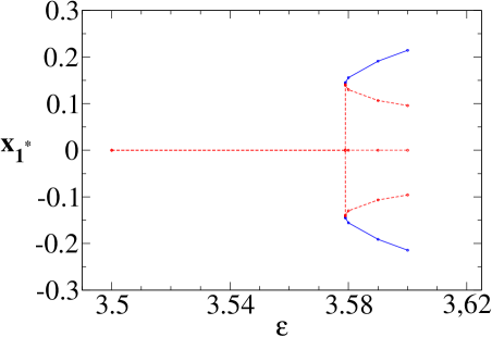
Figure 1: (Color online) Saddle-node bifurcation diagram showing the appearance of new equilibria and their stability for coupled system (4). The dashed (red) line corresponds to unstable fixed points, while the continuous (blue) line depicts stable ones.

For $\epsilon>0$, there is a critical value $\epsilon_{c}$ such that, for $\epsilon>\epsilon_{c}$, four new fixed points appear: two unstable and two asymptotically stable. In order to make numerical estimations from our model we make use of the extensive earlier research on the CV system [20, 25] embodied in the frequencies and amplitude relationships summarised in Table 1, so that we take $a_{1}/a_{5}\approx 1$, $a_{1}/a_{i}\approx 0.5$, for $i=\left\{2,3,4\right\}$.

Fig. 1 shows the bifurcation diagram for $x_{1}$, calculated for $a_{1}=0.5$, $a_{2}=1$, $f_{1}=1.1$, $f_{2}=0.3$ and $\alpha=1$. Note that for this range of $\epsilon>0$ the origin is always an unstable fixed point. The end of the oscillations is marked by the appearance of the new fixed points at $\epsilon\sim 3.578$. They are obtained from the set of algebraic equations:

$$\begin{array}[]{l c c}-x_{1}\alpha(\sqrt{x_{1}^{2}+y_{1}^{2}}-a_{1})-y_{1}\omega_{1}+\epsilon(x_{1}+x_{2})&=&0,\\ -y_{1}\alpha(\sqrt{x_{1}^{2}+y_{1}^{2}}-a_{1})+x_{1}\omega_{1}&=&0,\\ \\ -x_{2}\alpha(\sqrt{x_{2}^{2}+y_{2}^{2}}-a_{2})-y_{2}\omega_{2}+\epsilon(x_{1}+x_{2})&=&0,\\ -y_{2}\alpha(\sqrt{x_{2}^{2}+y_{2}^{2}}-a_{2})+x_{2}\omega_{2}&=&0.\end{array}$$ (7)

After some algebra, we obtain the relations:

$$\begin{array}[]{c c c}\omega_{1}(x_{1}^{2}+y_{1}^{2})&=&\epsilon y_{1}(x_{1}+x_{2}),\\ \omega_{2}(x_{2}^{2}+y_{2}^{2})&=&\epsilon y_{2}(x_{1}+x_{2}).\end{array}$$ (8)

Analysis of Eq. (8) combined with Eq. (7) shows that, for $\epsilon\ll 2\omega_{1}$ and $\epsilon\ll 2\omega_{2}$, the only fixed point is $(0,0,0,0)$. For sufficiently large values of $\epsilon$, we obtain four new fixed points. The fixed points can appear only in pairs of stable–unstable points. This is the saddle-node bifurcation route to OD, which occurs only for positive $\epsilon$.

We now define $x_{1}=r_{1}\cos{(\Phi_{1})}$, $y_{1}=r_{1}\sin{(\Phi_{1})}$, $x_{2}=r_{2}\cos{(\Phi_{2})}$, $y_{2}=r_{2}\sin{(\Phi_{2})}$, where $r_{1}^{2}=x_{1}^{2}+y_{1}^{2}$, $r_{2}^{2}=x_{2}^{2}+y_{2}^{2}$. As in our model $\omega_{1}\gg\omega_{2}$, $a_{2}>a_{1}$, which implies $(x_{1}^{0})^{2}\ll(x_{2}^{0})^{2}$. From Eq. (8) we obtain the equality:

$$\omega_{2}=\epsilon\cos{(\Phi_{2})}\sin{(\Phi_{2})}.$$ (9)

This is equivalent to the equation:

$$\frac{2\omega_{2}}{\epsilon}=\sin{(2\Phi_{2})}.$$ (10)

As $\sin{(2\Phi_{2})}\leq 1$, this means that we have new solutions to the algebraic equations (7) only when

$$\epsilon>2\omega_{2}.$$ (11)

Eq. (11) provides a simple and understandable analytic estimate of the critical value for the bifurcation.

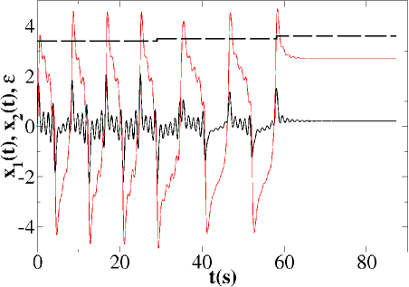
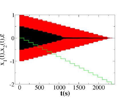
Figure 2: (Color online) Top: Time series of $x_{1}(t)$ (bold curve) and $x_{2}(t)$ from numerical simulations of the system (4), showing saddle-node OD. Parameter values were the same as in Fig. 1. The dashed line shows the step–wise variation of the coupling constant $\epsilon$ in a positive range. Note that after OD has occurred $\displaystyle\lim_{t\rightarrow\infty}\left\{x_{1}(t),x_{2}(t)\right\}>0$. Bottom: Time series of $x_{1}(t)$ and $x_{2}(t)$ from numerical simulations of the system (4), showing supercritical Hopf bifurcation OD. Parameter values were the same as in Fig. 1. The diagonal stepped line starting at the origin indicates how $\epsilon$ was varied in the negative range. In this case $\displaystyle\lim_{t\rightarrow\infty}\left\{x_{1}(t),x_{2}(t)\right\}=0$, after OD has occurred. Note the difference in abscissa timescales between the top and bottom parts of the figure.

Fig. 2 (top) illustrates a numerical simulation of the coupled oscillators (4) near criticality, showing how the oscillations evolve as $\epsilon$ is increased by steps of 0.1. We have established that, for the chosen parameter values, the oscillations die when $\epsilon_{c}\approx 3.578$, gratifyingly close to the $\epsilon_{c}\approx 4\pi f_{2}=3.77$ predicted by (11). The difference is attributable to the approximations made in deriving Eq. (11). Using the same values of parameters, we also performed numerical simulations for negative $\epsilon$, Fig. 2 (bottom), and found that OD occurs through supercritical Hopf bifurcation when $\epsilon\sim-1.88$, in agreement with the theoretical prediction (6).

We have also used the above mathematical tools to investigate the full model [20] with five coupled oscillators $(i=1,\ldots,5)$. Solutions of the algebraic equations

$$\begin{array}[]{c c l}0&=&-x_{i}q_{i}-y_{i}\omega_{i}+\epsilon\displaystyle\sum_{j=1}^{5}{x_{j}}\\ 0&=&-y_{i}q_{i}+x_{i}\omega_{i},\end{array}$$ (12)

correspond to the fixed points of (1) for five coupled oscillators. After some calculations we get the equations

$$\begin{array}[]{c c c}\omega_{i}(x_{i}^{2}+y_{i}^{2})&=&\epsilon y_{i}\sum{x_{j}}.\end{array}$$ (13)

We have found that, for $\epsilon>\epsilon_{c}$, where $\epsilon_{c}$ is some critical value, the system possesses four additional fixed points (two stable and two unstable).

Because $\omega_{i}=2\pi f_{i}$, and using the empirical physiological values (table 1) for the $f_{i}$’s and $a_{i}$’s mentioned above, we can use the inequalities $\omega_{5}<\omega_{4}<\omega_{3}<\omega_{2}<\omega_{1}$, and $a^{2}_{1}=a^{2}_{5}<a^{2}_{2}=a^{2}_{3}=a^{2}_{4}$, in order to obtain an analytic expression for $\epsilon_{c}$. The resulting approximate equations lead to the following relations for the systems’ fixed points: $\sum{x_{j}}\approx\omega_{1}a_{1}$; $x_{1}^{o}\approx y_{4}^{o}\approx y_{5}^{o}\approx 0$; $x_{3}^{o}\approx x_{4}^{o}\approx x_{5}^{o}\approx x_{*}$, where $x_{*}=\frac{a_{5}\alpha+\sqrt{a_{5}^{2}\alpha^{2}+4\omega_{1}a_{1}\alpha}}{2\alpha}$; $y_{1}\approx a_{1}$; $y_{2}^{o}=\frac{(a_{1}\omega_{1}-a_{2}^{2}\alpha)+\sqrt{(\omega_{1}a_{1}-\alpha a_{2}^{2})^{2}+4a_{2}^{3}\alpha\omega_{2}}}{2\omega_{2}}$

The new simplified equation (13), with $i=2$, is

$$\begin{array}[]{c c c}\omega_{2}((x_{2}^{o})^{2}+(y_{2}^{o})^{2})&=&\epsilon y_{2}^{o}x_{2}^{o}+\epsilon 3x_{*}y_{2}^{o}.\end{array}$$ (14)

The new stable fixed points are possible when

$$\begin{array}[]{c c c}y_{2}^{o}\epsilon^{2}+12x_{*}\omega_{2}\epsilon-4\omega_{2}^{2}y_{2}^{o}&>&0.\end{array}$$ (15)

The asymptotically stable equilibrium points are the new attractors of the dynamical system.

Using physiologically estimated values for the parameters (table 1) in (15) we obtain that $\epsilon_{c}\approx 0.468$. This result is in agreement with the numerical simulations shown on Fig. 3(a), where there is OD for $\epsilon\approx 0.47$.

We have also modeled the dynamics of the five-oscillator system for the given parameter values using analogue electronic circuits [28]. The result of Fig. 3(b) shows the experimental observation of OD in good qualitative agreement with both the theory and numerical simulations.

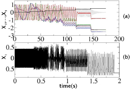
Figure 3: (Color online) Simulations of the coupled system (1) using five oscillators, as $\epsilon$ is increased in steps of 0.1. Parameter values are based on physiology (see text). (a) Numerical simulation showing the outputs from all five oscillators, exhibiting OD for $\epsilon\approx 0.47$. (b) Analogue electronic simulation, showing the output from the first oscillator $x_{1}$.

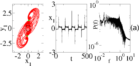
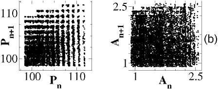
Figure 4: (Color online) Behavior of the coupled system (4) for $\epsilon=3.578$, very close to death. Row (a): Attractor in $x_{1}$-$y_{1}$ space, time series $x_{1}(t)$ and its Fourier transform. Row (b): First-return maps of the instantaneous period and amplitude signals.

We have found that, just before the onset of death, the 2-oscillator system (4) exhibits highly complex, quasiperiodic and chaotic, behavior. Fig. 4(a) plots the $x_{1}$-$y_{1}$ phase diagram when $\epsilon=3.578\approx\epsilon_{c}$. For comparison the circle in the background shows the limit cycle when $\epsilon=0$, and the two full (green) spots signal the place where the new fixed points will arise. The attractor’s structure, the seemingly random amplitudes of the time-series, the lengthening of the period with a square-root scaling, and the power-law-like spectrum, indicate that the system enters a chaotic regime just before it dies. Fig. 4(b) shows the first-return maps (FRM) of the discrete instantaneous period and amplitude signals obtained by sampling $x_{1}(t)$ at the peaks. We observe strong period and amplitude variability in the FRM, with the period showing a multimodal distribution. The amplitude of peaks has a more uniform distribution showing fewer preferred values, and the amplitude difference between successive peaks is distributed normally. In terms of the cardiovascular analogue this complex behavior might be seen as a predictor of imminent death of the cardio-respiratory coupled oscillations. Moreover, multimodal period distributions are typical of the time variability observed in other biological systems, e.g. the intermitotic time of human skeletal cells, and moments of change in the rotation direction of flagella [23]. It is evident that, at least in this kind of coupled biological system, the variability of the oscillations increases near the onset of global bifurcations.

Thus, OD in (1) can occur via both of the known routes. When $\epsilon$ is negative and below a critical value, the origin becomes asymptotically stable and the oscillations die at almost constant frequency, i.e. the Hopf bifurcation scenario. In the second mechanism, OD occurs when new fixed points appear on the former attractor after $\epsilon$ has surpassed a positive threshold: the amplitude remains almost constant while the frequency decreases with a square-root scaling in a saddle-node bifurcation.

When a system arrives in the OD regime it lies quiescent. Although apparently trivial, this state results from diverse complex interactions between the coupled elements that form the system, as we show in this Letter. Thus OD can be seen as another kind of complex collective motion, much in the same way as synchronization arises in complex coupled systems as a self-organized dynamics.

In order to complete the analysis of system (1) in this context we investigate the relationship between synchronization and OD by measuring the synchronization index [2], defined as: $\gamma_{1,1}=\left\langle\cos{\Psi_{1,1}}\right\rangle^{2}+\left\langle\sin{\Psi_{1,1}}\right\rangle^{2}$, where $\Psi_{1,1}$ is the relative phase difference between the oscillators. This index measures quantitatively the strength of 1:1 synchronization.

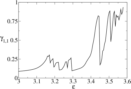
Figure 5: Synchronization index $\gamma_{1,1}$ as a function of the coupling strength $\epsilon$ for the system (1).

Fig. 5 shows the calculated values of $\gamma_{1,1}$ as a function of $\epsilon$ for the coupled system (1). Initially $\gamma_{1,1}$ is very small for low values of $\epsilon$ and it increases monotonically in a quasi-exponential fashion as $\epsilon$ is increased. However when $\epsilon$ reaches a value near 3.15, $\gamma_{1,1}$ no longer grows monotonically, but has alternating epochs of growth and decrease, corresponding to topological changes in the structure of the attractors of both oscillators that lead to complex transitions in the 1:1 synchronization state. These results suggest that the transient epochs of cardio-respiratory synchronization seen (for higher synchronization ratios) in many studies of resting humans, both awake [29, 30, 31] and asleep [32], may arise in part from changes in coupling, as well as from drifts in the natural frequencies and other parameters.

Finally, in order to explore the robustness of our results in a more realistic framework, we performed simulations of system (1) including the presence of stochastic forces, since they can lead to spurious detection of complex phenomena [33]. Our stochastic model is:

$$\begin{array}[]{c c l}\dot{x}_{i}&=&-x_{i}q_{i}-y_{i}\omega_{i}+\epsilon(x_{1}+x_{2})+D\xi_{x}\\ \dot{y}_{i}&=&-y_{i}q_{i}+x_{i}\omega_{i},\end{array}$$ (16)

where $\xi_{x}$ corresponds to white Gaussian noise with zero mean and variance $D^{2}$.

The simulation of Eq. (16) is shown in Fig. 6. The parameters used in this noisy equation are the same as those used for Eq. (1), besides $D=1.0$. In the top panel, $\epsilon$ was piecewise increased through a range of positive values, and OD was observed to occur at a value very close to the noiseless case, $\epsilon=3.57$. Similarly in Fig. 6 (bottom) $\epsilon$ was piecewise increased but now in the negative direction. OD was still observed, at a value near that of the noiseless case, $\epsilon=-1.8$. Thus the noise term in Eq. (16) does not eliminate, or change the nature of, the bifurcations leading to the appearance of OD; however, it influences the asymptotic value of the fixed points to which the system evolves.

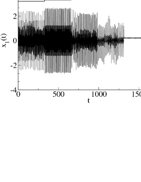
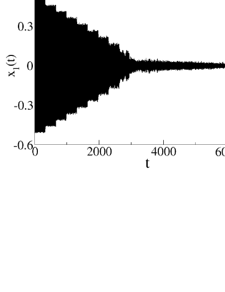
Figure 6: Temporal behavior of noisy system (16) as $\epsilon$ is varied piecewisely. Top: $\epsilon$ increases positively and OD is observed near $\epsilon$=3.57. Bottom: $\epsilon$ decreases negatively and OD is observed near $\epsilon$=-1.8. In both cases noise intensity is $D=1$.

In our study of OD we have obtained analytic relations predicting the onset of OD in the CV model, both for two and five coupled oscillators, using assumptions provided by experimental physiological measurements. In addition, all the theoretical results have been verified in numerical simulations. We have also observed partial OD [34] in our numerical model, where some oscillators die while others remain active. It occurs if the eigenvalues corresponding to certain variables $x_{i}$ and $y_{i}$ have negative real parts, while those corresponding to other oscillator variables do not have this property. For instance, this happens if $2\alpha a_{i}+\epsilon<0$. See Fig. 2 (bottom).

Discussions of OD usually focus on the strength of the coupling coefficient. The common phrase is that “for large couplings, amplitude death will take place”. However, now that we have analytic expressions for the critical value, also depending on other parameters, we can predict the onset of OD when different parameters are changed: OD is evidently a multi-parameter-sensitive phenomenon. It can be induced, not only by changes in couplings, but also by changes in the oscillator frequencies and amplitudes. For instance, the analytic conditions for OD given by (6) indicate that, if the amplitude parameters $a_{1}$ and $a_{2}$ decrease (in fact it is sufficient to decrease the largest one), then OD can occur for two coupled oscillators even when the coupling coefficient remains constant. The same can happen if the excitability parameter $\alpha$ is decreased below a critical value. Another interesting feature of OD inferred from (11) and (15) is that, if $\epsilon>0$, and $\epsilon>\epsilon_{c}$, new asymptotically stable fixed points can appear. Thus the oscillations die, but the dynamical variables can take non-zero asymptotic values. We remark that the critical value $\epsilon_{c}$ depends on the oscillators’ frequencies. That is, even for fixed coupling strength $\epsilon$, if the frequency of one of the oscillators falls below some critical value, then all the coupled system can stop dead. This behavior is true both for two or five coupled oscillators.

What are the implications of these results for the CVS? Given that (1) successfully models many features and states of the CVS, we may speculate that phenomena analogous to OD may also occur there. It would mean that, for certain parameter combinations, the mutual interactions between the cardiac, respiratory, myogenic, neurogenic and endothelial oscillators might serve to bring one or all of them to a halt – or at least to inhibit function. Treatment to prevent or remedy such a scenario might involve the use of drugs to modify some of the parameters $\alpha$, $a_{i}$ or $\omega_{i}$ so as to take the individual away from the regime of danger.

These results could also be applicable to coupled arrays of neurons in the brain. In the first demonstration of OD in a biological system Ozden et. al [10] coupled a man-made device to an array of real neurons and OD was provoked by taking the system into the strong-coupling regime. We hypothesize that similar results could be obtained in response to frequency changes, according to rules similar to (6) or (11). The system would not then need to be in the strong-coupling regime, which in some cases could damage sensitive biological tissue.

In summary, we have shown analytically and through simulations that OD in the CVS model (1) can occur via either of the known bifurcation mechanisms. Furthermore, OD can be induced, not only by an increase in coupling strength as conventionally accepted, but also by changes of e.g. amplitude and/or frequency. We have shown it to be sensitive to many different parameters. Connections between OD in the model, and phenomena in the CVS, appear possible but remain to be explored.

- [1] Sometimes known as amplitude death, which can be misleading where death occurs at finite oscillation amplitude.
- [2] \NamePikovsky A., Rosenblum M. and Kurths J. \BookSynchronization: A Universal Concept in Nonlinear Sciences \PublCambridge University Press, Cambridge, UK \Year2001
- [3] \NameBar-Eli, K. \REVIEWPhysica D141985242.
- [4] \NameCrowley M. and Epstein I. \REVIEWJ. Phys. Chem.9319892496.
- [5] \NameAronson D., Ermentrout B. and Kopell N. \REVIEWPhysica D411990403.
- [6] \NameZhu Y., Qian X. and Yang J. \REVIEWEurophys. Lett.82200840001.
- [7] \NameGallego B. and Cesso P. \REVIEWJ. Climate1420012815.
- [8] \NameZhai Y., Kiss I. and Hudson J. \REVIEWPhys. Rev. E692004026208.
- [9] \NameWei M. and Lun J. \REVIEWAppl. Phys. Lett.912007061121.
- [10] \NameOzden I., Venkataramani S., Long M., Connors B. and Nurmikko A. \REVIEWPhys. Rev. Lett.932004158102.
- [11] \NameHerrero R., Figueras M., Rius J., Pi. F. and Orriols G. \REVIEWPhys. Rev. Lett.8420005312.
- [12] \NameReddy D., Sen A. and Johnston G. \REVIEWPhys. Rev. Lett.8520003381.
- [13] \NameErmentrout B. \REVIEWPhysica D411990219;
- [14] \NameErmentrout B. and Kopell N. \REVIEWSIAM J. Appl. Math.501990125;
- [15] \NameMirollo R. and Strogatz S. \REVIEWJ. Stat. Phys.601990245;
- [16] \NameMatthews P. and Strogatz S. \REVIEWPhys. Rev. Lett.6519901701.
- [17] \NameReddy D., Sen A. and Johnston G. \REVIEWPhys. Rev. Lett.8019985109.
- [18] \NameAtay F. \REVIEWPhys. Rev. Lett.912003094101.
- [19] \NameKarnatak R., Ramaswamy R. and Prasad A. \REVIEWPhys. Rev. E762007035201.
- [20] \NameStefanovska A. and Bračič M. \REVIEWContemporary Phys.40199931.
- [21] \NameDe Monte S., d’Ovidio F. and Mosekilde E. \REVIEWPhys. Rev. Lett.902003054102.
- [22] \NameIvanov P., Amaral L., Goldberger A., Havlin S., Rosenblum M. Struzik Z. and Stanley H. E. \REVIEWNature3991999461.
- [23] \NameVolkov E. and Stolyarov M. \REVIEWBiol. Cybern.711994451.
- [24] \NameStefanovska A., Lotrič, M. B., Strle S. and Haken H. \REVIEWPhysiol. Meas.222001535.
- [25] \NameStefanovska A. \REVIEWIEEE Eng. Med. Biol. Mag.26200725.
- [26] The additional nitric oxide independent endothelial oscillatory process at about 0.007 Hz [25] does not affect the results reported in this paper.
- [27] \NameGlass L. and Mackey M. \BookFrom Clocks to Chaos: The Rhythms of Life \PublPrinceton University Press, Princeton, USA \Year2008.
- [28] \NameLuchinsky D., McClintock P. V. E. and Dykman M. \REVIEWRep. Progr. Phys.611998889.
- [29] \NameSchäfer C., Rosenblum M. G., Abel H. H. and Kurths J. \REVIEWPhys. Rev. E601999857.
- [30] \NameLotrič M. B. and Stefanovska A. \REVIEWPhysica A2832000451.
- [31] \NameKenwright D. A., Bahraminasab A., Stefanovska A. and McClintock P. V. E. \REVIEWEur. Phys. J. B652008425.
- [32] \NameBartsch R., Kantelhardt J., Penzel T. and Havlin S. \REVIEWPhys. Rev. Lett.982007054102.
- [33] \NameXu L., Chen Z., Hu K., Stanley H. and Ivanov P. \REVIEWPhys. Rev. E732006065201.
- [34] \NameLiu W., Xiao J. and Yang J. \REVIEWPhys. Rev. E722005057201.