Weakly Coupled Discretized Gravity

Gerhart Seidl

Institut für Theoretische Physik und Astrophysik
Universität Würzburg, D 97074 Würzburg, Germany

Abstract

We consider discretized gravity in 4+2 dimensions compactified on a disk of constant negative curvature. The curvature of the disk avoids the presence of dangerous ultra-light scalar modes but comes also along with a high multiplicity of states potentially jeopardizing a good strong-coupling behavior of the discretized theory. We demonstrate that for Standard Model matter propagating on the five-dimensional boundary submanifold of the disk, the strong coupling scale, as seen by an observer, can be parametrically larger than the local Planck scale. As a consequence, we obtain a description of weakly coupled discretized gravity on the boundary that can be compared with the continuum theory all the way up to the effective five-dimensional Planck scale.

1 Introduction

About a decade ago, the study of curved background geometries in more than four dimensions has led to the development of important ideas such as the Randall-Sundrum (RS) model [1, 2] and gauge gravity duality [3]. Solving Einstein’s equations for general curved backgrounds, however, is very difficult in practice. Discretized or lattice gravity [4], on the other hand, may be a possibility for describing gravity in extra-dimensional geometries at the level of an effective field theory (EFT) [5, 6] (for related work see, e.g., [7]) without the need to solve Einstein’s equations explicitly [8]. In fact, it has been shown that five-dimensional (5D) flat space lattice gravity gives a valid EFT of massive gravity up to energies above the compactification scale [5], while discretized gravity in 5D warped space works in the manifestly holographic regime [8, 9].

Minimal models of 5D discretized gravity face, however, a strong coupling phenomenon which forbids to take the continuum limit within a consistent EFT. This difficulty arises from the presence of an ultra-light mode with dangerous long-range interactions that prevent us from taking the large volume limit [5]. In contrast to this, the large volume limit can be taken in discretized 5D warped space-time [8, 9], but the EFT still gets, due to the light mode, early strongly coupled below the local Planck scale. A possible way out of this problem may be offered in discrete hyperbolic space. If we view the 5th dimension as the boundary of a six-dimensional (6D) hyperbolic disk, the light mode can become very heavy due to the hyperbolic curvature of the disk [10]. This can leave us on the 5D boundary with a theory of discretized gravity that is more weakly coupled than in minimal 5D models. In fact, phenomenological features of hyperbolic extra dimensions have been considered previously in [11] and collider implications were analyzed in [10, 12]. However, even on the hyperbolic disk, the strong coupling scale as seen by a brane-localized observer can become as large as that of the continuum theory only in the limit where all massive gravitons decouple above the local Planck scale [10].

In this paper, we consider a model for discretized gravity on a 6D hyperbolic disk with an EFT for massive gravitons on the 5D boundary that is meaningful at energies up to the effective 5D Planck scale. This is achieved by letting Standard Model (SM) matter propagate on the 5D boundary of the disk, just as in universal extra dimensions [13]. Compared with the previous case of an observer localized on a single point [10], the propagation of SM matter on the boundary implies KK number conservation, which shuts off the contribution of a high multiplicity of Kaluza-Klein (KK) levels to the tree-level scattering amplitudes of SM matter. This gives a theory of weakly coupled discretized gravity on the 5D boundary with a strong coupling scale that is parametrically larger than the local Planck scale. It thus becomes possible to compare the discretized theory on the boundary with the continuum theory all the way up to the effective 5D Planck scale.

The paper is organized as follows. In Sec. 2, we review the warped hyperbolic disk geometry. A rough discretization of the disk for the flat and the strongly warped case is next carried out in Sec. 3. Then, in Sec. 4, we give for these cases the strong coupling scale in pure gravity. In Sec. 5, we consider the EFT of massive gravitons as seen by an observer on the boundary of the disk. Finally, we present in Sec. 6 our summary and conclusions.

2 Disk geometry

We start by briefly reviewing 6D general relativity compactified to four dimensions on an orbifold $K_{2}/Z_{2}$, where $K_{2}$ is a two-dimensional disk of constant negative curvature. We follow here closely the more detailed description in [10]. In what follows, the 6D coordinates $x^{M}$ are labeled by capital Roman indices $M=0,1,2,3,5,6$ whereas Greek indices $\mu=0,1,2,3$ symbolize the usual four-dimensional (4D) coordinates $x^{\mu}$ and the Minkowski metric is $\eta_{MN}=\textrm{diag}(1,-1,\dots,-1)$. On the disk $K_{2}$, a point is given by polar coordinates $(r,\varphi)$, where $r=x^{5}$ and $\varphi=x^{6}$ with $r\in[0,L]$ and $\varphi\in[0,2\pi)$. In our notation, $r$ is the geodesic distance of the point $(r,\varphi)$ from the center and $L$ is the proper radius of the disk. We arrive at the orbifold $K_{2}/Z_{2}$ by assuming the orbifold projection $\varphi\rightarrow-\varphi$. This restricts the physical space on the disk to $(r,\varphi)\in[0,L]\times[0,\pi]$.

The 6D metric $\tilde{g}_{MN}$ for the curved disk is defined by the line element

$$ds^{2}=e^{2\sigma(r)}g_{\mu\nu}(x,r,\varphi)dx^{\mu}dx^{\nu}-dr^{2}-\frac{1}{v^{2}}\,\textrm{sinh}^{2}(v\cdot r)d\varphi^{2},$$ (1)

where $1/v$ is the curvature radius of the disk with $v>0$, $g_{\mu\nu}(x,r,\varphi)$ is the 4D metric with $x\equiv(x^{\mu})$, and $\sigma(r)=-w\cdot r$, where $w$ is the curvature scale for the warping. A comparison of our space with the Poincaré hyperbolic disk is given in [10]. Like in RS I [1], we have assumed in (1) orbifold boundary conditions with respect to $r$ at the center $r=0$ and at the boundary of the disk at $r=L$. While we identify the UV brane with the center at $r=0$, we have IR branes residing at the orbifold fixed points on the boundary at $r=L$.

We assume the Einstein-Hilbert action

$$\mathcal{S}=M_{6}^{4}\int d^{6}x\,\sqrt{|\tilde{g}|}(\tilde{R}-2\Lambda)$$ (2)

for gravity, where $\tilde{g}\equiv\det\tilde{g}_{MN}$, $M_{6}$ is the 6D Planck scale, $\Lambda$ the bulk cosmological constant, $\tilde{R}=\tilde{g}^{MN}\tilde{R}_{MN}$ the 6D curvature scalar, and $\tilde{R}_{MN}$ the 6D Ricci tensor. Expanding $g_{\mu\nu}$ in terms of small fluctuations around 4D Minkowski space as $g_{\mu\nu}=\eta_{\mu\nu}+h_{\mu\nu}$, we obtain, to quadratic order, the linearized kinetic part of the graviton Lagrangian density

$$\mathcal{S}_{\text{lin}}=\mathcal{S}_{\text{kin}}+\mathcal{S}_{\text{FP}}$$ (3)

with the kinetic term

$$\mathcal{S}_{\textrm{kin}}=M_{6}^{4}\int d^{6}x\,v^{-1}\textrm{sinh}(vr)\frac{1}{4}e^{2\sigma(r)}(\partial^{\mu}h^{\nu\kappa}\partial_{\mu}h_{\nu\kappa}-\partial^{\mu}h\partial_{\mu}h-2h^{\mu}h_{\mu}+2h^{\mu}\partial_{\mu}h),$$ (4)

where $h={h^{\mu}}_{\mu},h_{\nu}=\partial^{\mu}h_{\mu\nu}$, and $\mathcal{S}_{\text{FP}}$ is of Fierz-Pauli form [14, 15]

$$\mathcal{S}_{\textrm{FP}} = M_{6}^{4}\int d^{6}x\,v^{-1}\textrm{sinh}(vr)\Big{[}\frac{1}{4}e^{4\sigma(r)}(\partial_{r}h_{\mu\nu})(\eta^{\mu\nu}\eta^{\alpha\beta}-\eta^{\mu\alpha}\eta^{\nu\beta})(\partial_{r}h_{\alpha\beta})$$ (5)

$$\qquad\,\,+\frac{1}{4}e^{4\sigma(r)}v^{2}\textrm{sinh}^{-2}(vr)(\partial_{\varphi}h_{\mu\nu})(\eta^{\mu\nu}\eta^{\alpha\beta}-\eta^{\mu\alpha}\eta^{\nu\beta})(\partial_{\varphi}h_{\alpha\beta})\Big{]}.$$

As in [5], we have neglected the 4D vector, scalar, and radion degrees of freedom, and have assumed a gauge with $h_{5M}=h_{6M}=0$, for $M=0,1,\dots,6$.

3 Warped space discretization

Let us now consider the rough latticization of the disk $K_{2}$ as described in [10]. Different from earlier, however, we now include a non-trivial warp factor that can be large. The latticization of the disk is defined by a number sites and links, where $N$ sites, labeled as $i=1,2,\dots,N$, are placed on the boundary and one site, carrying the label $i=0$, is placed at the center ($r=0$) of the disk. The sites on the boundary of the disk are evenly spaced on a concentric circle with proper radius $L$ around the central site $i=0$, i.e. the $i$th site on the boundary has polar coordinates $(r,\varphi)=(L,i\cdot\Delta\varphi)$, where $\Delta\varphi=2\pi/N$. Two sites $i$ and $i+1$ on the boundary are connected by a link $(i,i+1)_{\textrm{link}}$, while the site $i=0$ in the center is connected to all $N$ sites on the boundary by links $(0,i)_{\textrm{link}}$. To implement a lattice gravity theory in terms of this triangulation, we will interpret the sites and links according to [4, 5, 6]. Here, each site $i$ is equipped with its own metric $g^{i}_{\mu\nu}$, which can be expanded around flat space as $g^{i}_{\mu\nu}=\eta_{\mu\nu}+h^{i}_{\mu\nu}$, where $\eta_{\mu\nu}$ is the usual 4D Minkowski metric. In a naive latticization of the linearized action $\mathcal{S}_{\textrm{lin}}$ in (5), we then replace the derivatives on the sites as

$$\partial_{\varphi}h_{\mu\nu}\rightarrow\frac{e^{-2wL}}{\Delta\varphi}(h_{\mu\nu}^{i+1}-h_{\mu\nu}^{i}),\quad\partial_{r}h_{\mu\nu}\rightarrow\frac{e^{-2wL}}{L}(h^{i}_{\mu\nu}-h_{\mu\nu}^{0}),\quad M_{6}^{4}\int dx^{5}dx^{6}\rightarrow M_{4}^{2}\sum_{i=0,1}^{N},$$ (6)

where it is always understood that the summation starts at $i=0$ for $\mathcal{S}_{\text{kin}}$ and at $i=1$ for $\mathcal{S}_{\text{FP}}$. In the case of zero warping, $w=0$, the local 4D effective Planck scale $M_{4}$ on each of the $N+1$ sites is related to $M_{6}$ and the usual 4D Planck scale $M_{\rm Pl}\simeq 10^{18}\>{\rm GeV}$ by $M_{4}^{2}=M_{6}^{4}A/N$ and $M_{\rm Pl}^{2}=M_{6}^{4}A=M_{4}^{2}N$, where $A=4\pi v^{-2}\sinh^{2}{(vL/2)}$ is the proper area of the disk. For strong warping, $w\gg v$ and $w\gg L^{-1}$, the graviton zero mode gets located at the center of the disk and we have, instead, $M_{4}\approx M_{\text{Pl}}$. The model possesses the graviton mass spectrum

$$M_{0}^{2}=0,\quad M_{n}^{2}=m_{*}^{2}\epsilon^{2}+4m^{2}\epsilon^{2}{\textrm{sin}}^{2}\frac{\pi n}{N},\quad M_{N}^{2}=(N\epsilon^{2}+1)m_{\ast}^{2}\epsilon^{2},$$ (7)

where $m_{*}=1/L$ and $m=Nv/2\pi\,\textrm{sinh}(vL)$ are the proper inverse lattice spacings in radial ($m_{*}$) and angular ($m$) direction, $n$ runs over $n=1,2,\dots,N-1$, and $\epsilon\equiv e^{-wL}$ is the warp factor. In the basis $(h_{\mu\nu}^{0},h_{\mu\nu}^{1},\dots,h_{\mu\nu}^{N})$, the corresponding canonically normalized graviton mass eigenstates read

$$M_{0}^{2} : \frac{1}{\sqrt{1+N\epsilon^{2}}}(1,\epsilon,\epsilon,\dots,\epsilon)\hat{H}^{0}_{\mu\nu}(x),$$

$$M_{n}^{2} : \frac{1}{\sqrt{N}}(0,1,e^{{\textrm{i}}\frac{2n\pi}{N}},e^{{\textrm{i}}\frac{4n\pi}{N}},\dots,e^{{\textrm{i}}\frac{2(N-1)n\pi}{N}})\hat{H}^{n}_{\mu\nu}(x),$$ (8)

$$M_{N}^{2} : \frac{1}{\sqrt{N(1+N\epsilon^{2})}}(N\epsilon,-1,-1,\dots,-1)\hat{H}^{N}_{\mu\nu}(x),$$

where we have, for simplicity, taken $N$ to be even. Note that irrespective of the warping, the $N-1$ eigenstates with mass-squares $M_{n}^{2}$ are all exactly located on the boundary of the disk. The profiles of the zero mode and of the $N$th massive mode, however, strongly depend on the choice of the warp factor. Consider first zero warping, $\epsilon=1$. In this case, the zero mode has a flat wave function and is mostly living on the boundary, whereas the heavy mode is peaked at the center of the disk. In contrast to this, for strong warping, $N\epsilon^{2}\ll 1$, the mode with mass $M_{N}$ gets pushed away from the center of the disk more towards the boundary. At the same time, we see that the zero mode becomes, instead, strongly localized at the center of the disk. We also observe that for $N\epsilon^{2}\ll 1$ a moderate increase of $N$ has barely any effect on the gravitational strength experienced at a single point on the boundary. This reproduces the feature of RS that the low-energy Planck scale depends only very weakly on the size of the warped extra dimension.

4 Strong coupling scale in pure gravity

In this section, we discuss the strong coupling behavior of the discretized model in the gravitational sector using the EFT for massive gravitons in [4, 5, 6].

To implement the EFT on the discretized disk $K_{2}$, we replace in (6) the differences $h^{i}_{\mu\nu}-h^{j}_{\mu\nu}$ between the graviton fields on two sites $i$ and $j$ that are connected by a link $(i,j)_{\textrm{link}}$ according to

$$h_{\mu\nu}^{i}-h_{\mu\nu}^{j}\,\,\rightarrow\,\,g_{\mu\nu}^{i}-\partial_{\mu}Y_{i,j}^{\alpha}\partial_{\nu}Y_{i,j}^{\beta}g^{j}_{\alpha\beta},\quad Y_{i,j}^{\mu}(x_{\mu})=x^{\mu}+A_{i,j}^{\mu}(x_{\mu})+\partial^{\mu}\phi_{i,j}(x_{\mu}),$$ (9)

in which $Y_{i,j}^{\mu}$ denotes a link field and $A_{i,j}^{\mu}$ and $\phi_{i,j}$ are the vector and scalar components of the Goldstone bosons that restore general coordinate invariances in the EFT (see [4, 5, 6]).

The kinetic Lagrangian of the gravitons is found by taking in (9) the links $(i,j)_{\textrm{link}}$ to be $(i,j)_{\textrm{link}}=(i,i-1)_{\textrm{link}}$, where $i=2,\ldots,N,N+1$, and $(i,j)_{\text{link}}=(i,0)_{\text{link}}$, where $i=1,2,\dots,N,$ and $N+1\equiv 1$. As a consequence, we obtain from $\mathcal{S}_{\text{FP}}$ in (5), after partial integration, the total action of the disk in position space

$$\mathcal{S}_{\rm disk} = \mathcal{S}_{\rm FP}+M_{6}^{4}\int{\rm d}^{6}x\,e^{-2wr}\big{(}h_{\mu\nu}\Box h_{\mu\nu}-m_{*}h_{\mu\nu}\Box\partial_{r}\phi-h_{\mu\nu}\Box\partial_{\varphi}\phi$$ (10)

$$\qquad\qquad\qquad+e^{-2wr}m_{*}^{2}(\Box\phi)^{3}+e^{-2wr}m^{2}(\Box\phi)^{3}\big{)},$$

where we have used the short-hand notation

$$e^{-4wr}m_{*}^{2}(\Box\phi)^{3}\rightarrow e^{-4wr}m_{*}^{2}(\Box\phi_{0,i})^{3},\quad e^{-4wr}m^{2}(\Box\phi)^{3}\rightarrow e^{-4wr}m^{2}(\Box\phi_{i,i-1})^{3}.$$ (11)

A linear Weyl-rescaling [5, 9]

$$h_{\mu\nu}\rightarrow h_{\mu\nu}^{\prime}=h_{\mu\nu}+e^{-2wr}\eta_{\mu\nu}(m_{*}\partial_{r}+m^{2}\partial_{\varphi})\phi$$ (12)

removes the kinetic mixing between $h_{\mu\nu}$ and $\phi$ in (10). In momentum space, for large $N$ and $m_{\ast}\gtrsim m$, the dominant contribution to the massive graviton scattering amplitude is then given by the tri-linear derivative coupling

$$M_{4}^{2}\frac{m_{*}^{2}\epsilon^{4}}{\sqrt{N}}(\Box\Phi_{n})(\Box\Phi_{m})(\Box\Phi_{-n-m})=\frac{1}{\sqrt{N}M_{4}m_{*}^{4}\epsilon^{5}}(\Box\hat{\Phi}_{n})(\Box\hat{\Phi}_{m})(\Box\hat{\Phi}_{-n-m}),$$ (13)

where we have expanded the scalar components of the Goldstone fields belonging to the links $(i,0)_{\textrm{link}}$ as $\phi_{i,0}=\frac{1}{\sqrt{N}}\sum_{n=1}^{N}e^{{\rm i}2\pi i\cdot n/N}\Phi_{n}$ with the definitions $\hat{\Phi}_{-n}=\hat{\Phi}_{N-n}$ and $\hat{\Phi}_{0}=\hat{\Phi}_{N}$, introduced the canonically normalized fields as $\hat{h}_{\mu\nu}=e^{-wr}h_{\mu\nu}$ and $\hat{\Phi}_{n}=\epsilon^{3}M_{4}m_{*}^{2}\Phi_{n}$, and used $\epsilon=e^{-wL}$ for the warp factor. From the amplitude for $\hat{\Phi}_{n}-\hat{\Phi}_{m}$ scattering, we hence find for the discrete disk geometry approximately the strong coupling scale

$$\Lambda=(\sqrt{N}M_{4}m_{*}^{4})^{1/5}\epsilon.$$ (14)

For zero warping, the above equation becomes $\Lambda=(M_{\rm Pl}m_{*}^{4})^{1/5}$, which is independent from the number of sites $N$ on the boundary and identical with the strong coupling scale in the theory of a single massive graviton with mass $m_{*}$ [4]. Since all graviton modes (except for the zero mode) have received a mass of the order the inverse proper radius of the disk $m_{*}$, no dangerous light modes are present anymore and we take in (14) the large $N$ limit. If, e.g., $N=100$ and $m_{*}\rightarrow M_{4}$, we find a strong coupling scale $\Lambda\approx 1.5\times\epsilon M_{4}$ that is somewhat larger than the (warped) local Planck scale on the boundary $\epsilon M_{4}$. If we wish to compare with the continuum theory, however, we cannot actually take the limit $m_{*}\rightarrow M_{4}$. The reason is that this would push all the graviton states above the local Planck scale $\epsilon M_{4}$ at which the continuum theory gets strongly coupled (cf. (7)). When matching between the lattice and the continuum theory, we therefore always have to take $m_{\ast}<M_{4}$. The inverse lattice spacing in angular direction, $m$, on the other hand, can be made as large as $M_{4}$. The idea being that $m\rightarrow M_{4}$ practically represents a “continuum limit” of the boundary submanifold.

In estimating the strong coupling scales, we will always assume that unwanted uneaten pseudo-Nambu-Goldstone bosons from the mesh of links acquire large masses from invariant plaquette terms that are added to the action [4] and lead to a decoupling of these states. Moreover, the strong coupling scale in (14) has been estimated in pure gravity only. In Sec. 5, we will take the coupling to matter into account and determine the strong coupling scale that is actually seen by an observer made of SM matter propagating on the 5D boundary submanifold of the disk.

5 Coupling to matter

Let us next determine the observed strong coupling scale for SM matter propagating on the boundary of the disk. Previously, we have studied the case where the SM is located on a single point on the boundary of the disk [10]. In this case, the local interaction ensures that the KK scalar components of the Goldstones couple all with equal strength to matter. Due to the high multiplicity of these states, this leads to an observed strong coupling scale that can be at most as large as the local Planck scale $\epsilon M_{4}$.

Different from this scenario, we will now assume that the SM matter propagates as zero modes on the 5D boundary $(r,\varphi)=(L,\varphi)$ of the disk as in the universal extra dimension scenario. From (3), we find that SM matter will then interact on the boundary of the disk with gravity as (see also [17])

$$\mathcal{S}_{\rm int}\approx\frac{1}{M_{\text{Pl}}}\int d^{4}x\,dy\,\frac{1}{R}T^{\mu\nu}\Big{(}\hat{H}^{0}_{\mu\nu}+\frac{1}{\epsilon}\sqrt{\frac{1+N\epsilon^{2}}{N}}\sum_{n}e^{-{\rm i}n\cdot y/R}\hat{H}^{n}_{\mu\nu}-\frac{1}{\epsilon\sqrt{N}}\hat{H}^{N}_{\mu\nu}\Big{)}+{\rm h.c.},$$ (15)

where $T^{\mu\nu}$ is the SM stress-energy tensor, $y\rightarrow i\cdot a_{\varphi}$ ($i=1,2,\dots$) is the coordinate of the 5D submanifold on the boundary, $dy\rightarrow a_{\varphi}$, and $R$ is the proper length of the boundary. On the disk $K_{2}$, $n$ would run from $1$ to $N-1$, but after orbifolding we have $n=1,\dots,\frac{N}{2}-1$ (for $N$ even). We will work here, for simplicity, with the states found in the discretization of the disk $K_{2}$ in Sec. 3, with the understanding that we actually have to finally impose orbifold boundary conditions as explained in Sec. 2 for the continuum theory.

We see from (15) that SM matter couples with gravitational strength $M_{\textrm{Pl}}^{-1}$ to the graviton zero mode $\hat{H}^{0}_{\mu\nu}$ and to the heavy modes $\hat{H}^{n}_{\mu\nu}$ roughly with strengths $\lesssim(\epsilon M_{\text{Pl}})^{-1}$ (for small $N$). For $m_{*}^{2}\gtrsim m$, the Weyl rescaling in (12) corresponds in momentum basis approximately to the change of the canonically normalized fields

$$\hat{H}^{n}_{\mu\nu}\rightarrow\hat{H}^{n}_{\mu\nu}+\eta_{\mu\nu}\hat{\Phi}_{-n},$$ (16)

where $n=1,\dots,N$, while $\hat{H}^{0}_{\mu\nu}$ has no kinetic mixing with the Goldstones. The Weyl rescaling in (16) introduces in $\mathcal{S}_{\text{int}}$ the matter-Goldstone interactions

$$\mathcal{S}^{\Phi}_{\text{int}}\approx\frac{1}{\epsilon M_{\text{Pl}}}\int d^{4}x\,dy\frac{1}{R}T\Big{(}\sqrt{\frac{1+N\epsilon^{2}}{N}}\sum_{n}e^{-{\rm i}n\cdot y/R}\hat{\Phi}_{-n}+\frac{1}{\sqrt{N}}\hat{\Phi}_{0}\Big{)}+{\rm h.c.},$$ (17)

where $T=\text{Tr}(T_{\mu\nu})$ and $\hat{\Phi}_{0}=\hat{\Phi}_{N}$ (see Sec. 4). Integrating now over $y$, we obtain in the 4D effective low-energy theory the interaction Lagrangian

$$\mathcal{S}^{\Phi}_{\text{int}}\approx\frac{1}{\epsilon M_{\text{Pl}}}\int d^{4}x\,T\sum_{n}\mathcal{F}^{n}\hat{\Phi}_{-n}+{\rm h.c.},$$ (18)

where $\mathcal{F}^{n}$ is a form factor and $n$ starts now from zero. The important point is that for SM matter propagating on the boundary, KK number conservation implies $\mathcal{F}^{0}\sim 1/\sqrt{N}$ but $\mathcal{F}^{n}=0$ for $n\neq 0$. If the SM fields were, instead, localized on a single point on the boundary [10], we would have $\mathcal{F}^{n}\sim 1$ for all $n$, i.e. a universal coupling of SM matter to a high multiplicity of Goldstones.

Let us next denote by $\psi^{n}$ the KK resonances of some SM field. The interactions of $\psi_{i}$ and $\psi_{j}$ with the Goldstones $\hat{\Phi}_{-n}$ are then described by (18), with the replacements $T\rightarrow T^{ij}$ and $\mathcal{F}^{n}\rightarrow\mathcal{F}^{ijn}$, where $T^{ij}$ is the trace of the energy-stress tensor for the fields $\psi_{i}$ and $\psi_{j}$, while $\mathcal{F}^{ijn}$ is the corresponding form factor describing the coupling of $T^{ij}$ with $\hat{\Phi}_{-n}$. For the zero modes of the matter fields $i=j=0$ we have $T^{00}=T$ and $\mathcal{F}^{00n}=\mathcal{F}^{n}$. Feynman rules for this case with gravity and matter on the boundary can be derived as in [18] (cf. [19]). Again, KK number conservation will give $\mathcal{F}^{ijn}\sim\sqrt{(1+N\epsilon^{2})/N}$ only for $i+j=n$, whereas $\mathcal{F}^{ijn}=0$ otherwise.

We are now in a position to estimate the strong coupling scale associated with processes involving SM KK resonances $\psi_{i}$ and Goldstones $\hat{\Phi}_{n}$. At tree level, we will restrict to the three example processes shown in Fig. 1: (a) $\psi_{i_{1}},\psi_{i_{2}}\rightarrow\psi_{j_{1}},\psi_{j_{2}}$, (b) $\psi_{i_{1}},\psi_{i_{2}}\rightarrow\psi_{j_{1}},\dots,\psi_{j_{4}}$, and (c) $\psi_{i_{1}},\dots,\psi_{i_{4}}\rightarrow\psi_{j_{1}},\dots,\psi_{j_{4}}$. In what follows, we assume that the $\psi_{i}$ are fermions. Let $E$ be the typical energy of the external particles. The largest matter-Goldstone vertex factors are those involving $\hat{\Phi}_{n\neq 0}$ and small $N$, which are of the order $E/\epsilon M_{\text{Pl}}$. Each three-Goldstone vertex, on the other hand, contributes to a diagram a factor $E^{6}/\sqrt{N}M_{4}m_{*}^{4}\epsilon^{5}$. We will perform a conservative estimate and assume for the matter-Goldstone vertices this limit. One should, however, keep in mind that the actual couplings of the SM fermion states to $\hat{\Phi}_{0}$ are smaller and suppressed by a factor $1/\sqrt{N}$ with respect to the couplings that we will use below.

Figure 1: Scattering of KK fermions via Goldstone modes at tree level. KK number conservation at the matter-Goldstone vertices switches off the high multiplicity of internal states.

We then obtain for the scattering amplitude $\mathcal{A}$ of diagram (a) roughly

$$\mathcal{A}\sim\left(\frac{E}{\epsilon M_{\text{Pl}}}\right)^{2}\frac{1}{E^{2}}=\frac{1}{\epsilon^{2}M_{\text{Pl}}^{2}}.$$ (19)

From (13), we find that the amplitude for diagram (b) is given by

$$\mathcal{A}\sim\left(\frac{E}{\epsilon M_{\text{Pl}}}\right)^{3}\left(\frac{1}{E^{2}}\right)^{3}\frac{E^{6}}{\sqrt{N}M_{4}m_{*}^{4}\epsilon^{8}}=\frac{E^{3}}{\sqrt{N}M_{\text{Pl}}^{3}M_{4}m_{*}^{4}\epsilon^{8}},$$ (20)

where we have used momentum conservation. Similarly, we arrive for diagram (c) at the amplitude

$$\mathcal{A}\sim\left(\frac{E}{\epsilon M_{\text{Pl}}}\right)^{4}\frac{E^{12}}{NM_{4}^{2}m_{*}^{8}\epsilon^{10}}\left(\frac{1}{E^{2}}\right)^{5}=\frac{E^{6}}{NM_{\text{Pl}}^{4}M_{4}^{2}m_{*}^{8}\epsilon^{14}}.$$ (21)

Note that KK number conservation ensures that the amplitudes are independent from $N$. This is completely different from [10], where, for the SM located at a single point on the boundary of the disk, the amplitudes corresponding to the diagrams (a), (b), and (c), would scale as $N,N^{2},$ and $N^{3}$, respectively. We thus estimate that the strong coupling scales associated with the diagrams in Fig. 1 become approximately

$$\text{(a)}\>:\>\Lambda\rightarrow\epsilon M_{\text{Pl}},\qquad\text{(b)}\>:\>\Lambda\rightarrow(\sqrt{N}M_{\text{Pl}}^{3}M_{4}m_{\ast}^{4})^{\frac{1}{8}}\epsilon,\qquad\text{(c)}\>:\>\Lambda\rightarrow(\sqrt{N}M_{\text{Pl}}^{2}M_{4}m_{*}^{4})^{\frac{1}{7}}\epsilon.$$ (22)

In the limit $m_{*}\rightarrow M_{4}$, the strong coupling scale $\Lambda$ becomes for both zero ($\epsilon=1$) and strong warping ($\epsilon\ll 1$) larger than the local Planck scale $M_{4}$.

Let us next look at quantum corrections to the scattering amplitudes. Consider for this purpose the 1-loop diagrams (a) and (b) in Fig. 2.

Figure 2: One loop corrections to the amplitude in Fig. 1 (a). KK number conservation requires $i_{1}+i_{2}=j_{1}+j_{2}=n$.

The diagrams give rise to the loop expansion parameters

$$\text{(a)}\>:\>\epsilon_{1}=\frac{1}{16\pi^{2}}\left(\frac{E}{M_{\text{Pl}}}\right)^{2}N_{\text{KK}}(E),\qquad\text{(b)}\>:\>\epsilon_{2}=\frac{1}{16\pi^{2}}\left(\frac{E^{5}}{\sqrt{N}M_{4}m_{*}^{4}\epsilon^{5}}\right)^{2}N_{\text{KK}}(E),$$ (23)

where $N_{\text{KK}}(E)$ is the number of KK states below $E$. The boundary has a warped compactification scale $M_{c}=1/R=2\epsilon m/N$. With $N_{\text{KK}}(E)=ER$, we find that the loop expansion parameters in (23) imply for zero warping ($\epsilon=1$) the strong coupling scales

$$\text{(a)}\>:\>\Lambda\rightarrow(16\pi^{2})^{\frac{1}{3}}M_{4},\qquad\text{(b)}\>:\>\Lambda\rightarrow(16\pi^{2})^{\frac{1}{11}}(M_{4}^{3}m_{*}^{8})^{\frac{1}{11}}\qquad(\epsilon=1)$$ (24a)

where we have used the 5D flat space relations $$M_{4}=(M_{\text{Pl}}^{2}/R)^{\frac{1}{3}}=M_{\text{Pl}}/\sqrt{N} N\epsilon^{2}\ll 1$$. Likewise, in the strongly warped case (), it follows from (24) that the theory would get strong coupled at

$$\text{(a)}\>:\>\Lambda\rightarrow(16\pi^{2})^{\frac{1}{3}}(M_{\text{Pl}}^{2}/R)^{\frac{1}{3}},\qquad\text{(b)}\>:\>\Lambda\rightarrow(16\pi^{2})^{\frac{1}{11}}(M_{\text{Pl}}^{2}m_{*}^{8}m)^{\frac{1}{11}}\epsilon\qquad(\epsilon\ll 1)$$ (24b)

where we have applied the warped space relation $M_{4}\approx M_{\text{Pl}}$. For $m_{*},m\rightarrow M_{4}$, diagram (b) then leads for a general warp factor to a strong coupling scale

$$\Lambda\approx 1.5\times\epsilon M_{4},$$ (25)

which is larger than the local Planck scale $\epsilon M_{4}$. This is similar to the scale that follows from Goldstone boson scattering in (14) in the same limit. Again, we cannot really take $m_{*}\rightarrow M_{4}$, since this would lead to a decoupling of all massive graviton states above the local Planck scale. But having $m_{*}$ somewhat smaller than $M_{4}$, allows us to compare the lattice gravity model with the continuum theory all the way up to the warped strong coupling scale $\epsilon M_{4}$ of the effective 5D continuum theory on the boundary.

Let us see how many KK gravitons we can actually fit in below $\epsilon M_{4}$. In Fig. 3, we show the maximum number $n_{\text{max}}$ of KK gravitons with masses below the 5D effective Planck scale on the boundary, $\epsilon M_{4}$, for both the flat and the strongly warped case. For nonzero warping, we have assumed a warp factor $\epsilon=10^{-12}$, leading to a local Planck scale on the boundary of the order $10^{3}\,\text{TeV}$. In Fig. 3, the left panel depicts the $n_{\text{max}}$ as a function of the local Planck scale $M_{4}$ and the right panel as a function of the warped compactification scale $M_{c}\simeq 1/R$ of the 5D boundary. The dashed lines in the figures indicate that above $10^{2}-10^{3}$ KK states the theory with the SM in universal extra dimensions would become non-perturbative at the one-loop level [13, 20], i.e. we have always to restrict in any case to $n_{\text{max}}\lesssim 10^{2}-10^{3}$ (around a TeV, $n_{\text{max}}$ it is closer to $10^{2}$ because of the running of the QCD coupling constant). In both graphs, we have always set $m=M_{4}$ to practically achieve the “continuum limit” on the boundary in the sense of Sec. 4. The curvature scale of the disk $m_{*}<M_{4}$, has been chosen in such a way that the smaller of the two strong coupling scales estimated in (14) and case (b) in (24) becomes equal to some scale $a\cdot M_{4}>M_{4}$, where $a$ is a positive number larger than one. In Fig. 3, $a$ takes for both graphs from top to bottom in this order the values $a=1.0,1.15,1.30,1.45,1.55,1.58$. One can see that the larger $a$, the smaller $n_{\text{max}}$, corresponding to an increasing number of KK states that decouple above $\epsilon M_{4}$, although this difference becomes marginal for $n_{\text{max}}\gg 1$. Having a number of about $n_{\text{max}}=\mathcal{O}(10^{2})$ KK states below the strong coupling scale requires therefore in the flat case the local Planck scale to be in the range

$$10^{16}\,\text{GeV}\lesssim M_{4}\lesssim 10^{17}\,\text{GeV}\quad(\epsilon=1).$$ (26)

For $n_{\text{max}}\gtrsim\mathcal{O}(10)$, the strong coupling scale set by the loop in diagram (b) in Fig. 2 dominates by dropping below that given in (14) and scales like $n_{\text{max}}\sim\epsilon M_{4}/M_{c}$. Therefore, going for the warped case in Fig. 3 to warp factors $\epsilon<10^{-13}$ will allow only a few states $n_{\text{max}}\lesssim\mathcal{O}(10)$ below $\epsilon M_{4}$. A perturbative model with about $\sim 10^{2}$ states below the local Planck scale $\epsilon M_{4}$ therefore requires warp factors and warped boundary compactification scales of the orders

$$\epsilon\gtrsim 10^{-12},\quad M_{c}\gtrsim 10\,\text{TeV}.$$ (27)

To solve the gauge hierarchy problem, one may therefore have to resort to supersymmetry. In total, we observe for the ranges of parameters in (26) and (27) that we can have a number of about $\mathcal{O}(10^{2})$ KK graviton states with a strong coupling scale as large as $\epsilon M_{4}$. This allows to compare the lattice theory with the effective 5D continuum theory on the boundary up to the effective warped 5D Planck scale $\epsilon M_{4}$.

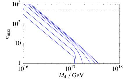
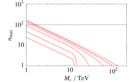
Figure 3: Maximum number of KK gravitons below the fundamental scale $M_{4}$ (see text) for the flat (left panel) and warped case (right panel). In the warped case, we have assumed a warp factor $\epsilon=10^{-12}$.

6 Summary and conclusions

In this paper, we have studied discretized gravity in a 6D geometry, where the two extra dimensions have been compactified on a hyperbolic disk. We have studied for the warped case the extreme limit of only two (or three) lattice sites in radial direction but with a smooth discretization and many sites on the boundary.

Working on the hyperbolic disk has the advantage that light states endangering a good strong coupling behavior of the discretized theory can be made massive by switching on the hyperbolic curvature. We have estimated the strong coupling scale of discretized as seen by an observer made of SM matter propagating on the 5D boundary of the disk. We found that the observed strong coupling scale can be parametrically larger than the Planck scale of the 5D effective continuum theory. This is due to KK number conservation which shuts off the high multiplicity of KK states that would otherwise contribute to tree level scattering amplitudes for an observer localized at a single point. We have estimated the range of parameters necessary for a theory of about $\sim 10^{2}$ massive gravitons in discretized gravity to be perturbative up to the effective 5D Planck scale for general warping. For these parameters, the discretized gravity theory on the boundary admits a comparison with the continuum theory all the way up to the strong coupling scale of the effective 5D continuum theory.

It would be interesting, e.g., to see how our results could be used for the formulation of a weakly coupled discrete version of the usual RS model as an effective theory, to compare them to theories dual to large-$N$ quantum field theories [21], and to apply them to modifications of gravity with relation to cosmology [22, 23].

References

- [1] L. Randall and R. Sundrum, Phys. Rev. Lett. 83 (1999) 3370.
- [2] L. Randall and R. Sundrum, Phys. Rev. Lett. 83 (1999) 4690.
- [3] J.M. Maldacena, Adv. Theor. Math. Phys. 2 (1998) 231 [Int. J. Theor. Phys. 38 (1999) 1113]; S.S. Gubser, I.R. Klebanov and A.M. Polyakov, Phys. Lett. B 428 (1998) 105; E. Witten, Adv. Theor. Math. Phys. 2 (1998) 253; O. Aharony, S.S. Gubser, J.M. Maldacena, H. Ooguri and Y. Oz, Phys. Rept. 323 (2000) 183.
- [4] N. Arkani-Hamed, H. Georgi and M.D. Schwartz, Annals Phys. 305 (2003) 96.
- [5] N. Arkani-Hamed and M.D. Schwartz, Phys. Rev. D 69 (2004) 104001.
- [6] M.D. Schwartz, Phys. Rev. D 68 (2003) 024029.
- [7] N. Boulanger, T. Damour, L. Gualtieri and M. Henneaux, Nucl. Phys. B 597 (2001) 127; T. Damour, I.I. Kogan and A. Papazoglou, Phys. Rev. D 66 (2002) 104025; N. Kan and K. Shiraishi, Class. Quant. Grav. 20 (2003) 4965; Prog. Theor. Phys. 111 (2004) 745; C. Deffayet and J. Mourad, Class. Quant. Grav. 21 (2004) 1833; G. Cognola, E. Elizalde, S. Nojiri, S. D. Odintsov and S. Zerbini, Mod. Phys. Lett. A 19 (2004) 1435.
- [8] L. Randall, M.D. Schwartz and S. Thambyapillai, JHEP 0510 (2005) 110.
- [9] J. Gallicchio and I. Yavin, JHEP 0306 (2006) 079.
- [10] F. Bauer, T. Hallgren and G. Seidl, Nucl. Phys. B 781, 32 (2007).
- [11] N. Kaloper, J. March-Russell, G. D. Starkman and M. Trodden, Phys. Rev. Lett. 85, 928 (2000); G. D. Starkman, D. Stojkovic and M. Trodden, Phys. Rev. Lett. 87, 231303 (2001).
- [12] H. Melbeus and T. Ohlsson, JHEP 0808, 077 (2008).
- [13] T. Appelquist, H. C. Cheng and B. A. Dobrescu, Phys. Rev. D 64, 035002 (2001).
- [14] See, e.g., G. ’t Hooft and M.J.G. Veltman, Annales Poincaré Phys. Theor. A 20 (1974) 69; M.J.G. Veltman, in Les Houches 1975: Methods in Field Theory, North-Holland, Amsterdam (1976); P. Van Nieuwenhuizen, Phys. Rept. 68 (1981) 189.
- [15] M. Fierz and W. Pauli, Proc. Roy. Soc. Lond. A 173 (1939) 211.
- [16] G. Dvali, O. Pujolas and M. Redi, Phys. Rev. Lett. 101, 171303 (2008) [arXiv:0806.3762 [hep-th]].
- [17] H. Davoudiasl, J. L. Hewett and T. G. Rizzo, Phys. Rev. Lett. 84, 2080 (2000) [arXiv:hep-ph/9909255].
- [18] C. Macesanu, A. Mitov and S. Nandi, Phys. Rev. D 68, 084008 (2003).
- [19] T. Han, J. D. Lykken and R. J. Zhang, Phys. Rev. D 59, 105006 (1999); G.F. Giudice, R. Rattazzi and J.D. Wells, Nucl. Phys. B 544 (1999).
- [20] Y. Nomura, Phys. Rev. D 65, 085036 (2002).
- [21] E. Kiritsis and V. Niarchos, arXiv:0808.3410 [hep-th].
- [22] G. R. Dvali, G. Gabadadze and M. Porrati, Phys. Lett. B 484, 112 (2000) [arXiv:hep-th/0002190].
- [23] T. Ohl and A. Schenkel, arXiv:0810.4885 [hep-th].