Five types of blow-up in a semilinear
fourth-order reaction-diffusion equation:
an analytic-numerical approach

Abstract.

Five types of blow-up patterns that can occur for the 4th-order semilinear parabolic equation of reaction-diffusion type

$$\textstyle{u_{t}=-\Delta^{2}u+|u|^{p-1}u\quad\mbox{in}\quad\mathbb{R}^{N}\times(0,T),\,\,p>1,\quad\lim_{t\to T^{-}}\sup_{x\in\mathbb{R}^{N}}|u(x,t)|=+\infty,}$$

are discussed. For the semilinear heat equation $u_{t}=\Delta u+u^{p}$, various blow-up patterns were under scrutiny since 1980s, while the case of higher-order diffusion was studied much less, regardless a wide range of its application. The types of blow-up include:

(i) Type I(ss): various patterns of self-similar single point blow-up, including those, for which the final time profile $|u(\cdot,T^{-})|^{N(p-1)/4}$ is a measure;

(ii) Type I(log): self-similar non-radial blow-up with angular logarithmic TW swirl;

(iii) Type I(Her): non self-similar blow-up close to stable/centre subspaces of Hermitian operators obtained via linearization about constant uniform blow-up pattern;

(iv) Type II(sing): non self-similar blow-up on stable/centre manifolds of a singular steady state in the supercritical Sobolev range $p\geq p_{\rm S}=\frac{N+4}{N-4}$ for $N>4$; and

(v) Type II(LN): non self-similar blow-up along the manifold of stationary generalized Loewner–Nirenberg type explicit solutions in the critical Sobolev case $p=p_{\rm S}$, when $|u(\cdot,T^{-})|^{N(p-1)/4}$ contains a measure as a singular component.

All proposed types of blow-up are very difficult to justify, so formal analytic and numerical methods are key in supporting some theoretical judgements.

1. From second-order to higher-order blow-up R–D models: a PDE route from XXth to XXIst century

1.1. The RDE–4 and applications

This paper is devoted to a description of blow-up patterns for the fourth-order reaction-diffusion equation (the RDE–4 in short)

(1.1) $$\textstyle{u_{t}=-\Delta^{2}u+|u|^{p-1}u\quad\mbox{in}\quad\mathbb{R}^{N}\times(0,T),\quad\mbox{where}\quad p>1,}$$

where $\Delta$ stands for the Laplacian in $\mathbb{R}^{N}$. This has the bi-harmonic diffusion $-\Delta^{2}$ and is a higher-order counterpart of classic second-order PDEs, which we begin our discussion with. For applications of such higher-diffusion models, see short surveys and references in [3, 40]. In general, higher-order semilinear parabolic equations arise in many physical applications such as thin film theory, convection-explosion theory, lubrication theory, flame and wave propagation (the Kuramoto-Sivashinsky equation and the extended Fisher-Kolmogorov equation), phase transition at critical Lifschitz points, bi-stable systems and applications to structural mechanics; the effect of fourth-order terms on self-focusing problems in nonlinear optics are also well-known in applied and mathematical literature. For a systematic treatment of extended KPPF-equations, see Peletier–Troy [76].

Note that another related fourth-order one-dimensional semilinear parabolic equation

(1.2) $$u_{t}=-u_{xxxx}-[(2-(u_{x})^{2})u_{x}]_{x}-\alpha u+q{\mathrm{e}}^{su},$$

where $\alpha$, $q$ and $s$ are positive constants obtained from physical parameters, occurs in the Semenov-Rayleigh-Benard problem [53], where the equation is derived in studying the interaction between natural convection and the explosion of an exothermically-reacting fluid confined between two isothermal horizontal plates. This is an evolution equation for the temperature fluctuations in the presence of natural convection, wall losses and chemistry. It can be considered as a formal combination of the equation derived in [44] (see also [5]) for the Rayleigh-Benard problem and of the Semenov-like energy balance [79, 16] showing that natural convection and the explosion mechanism may reinforce each other; see more details on physics and mathematics of blow-up in [40]. In a special limit, (1.2) reduces to the generalized Frank-Kamenetskii equation (see [3] for blow-up stuff)

(1.3) $$u_{t}=-u_{xxxx}+{\mathrm{e}}^{u},$$

which is a natural extension of the classic Frank-Kamenetskii equation; see below.

Equation (1.1) can be considered as a non-mass-conservative counterpart of the well-known limit unstable Cahn–Hilliard equation from phase transition,

(1.4) $$u_{t}=-u_{xxxx}-(|u|^{p-1}u)_{xx}\quad\mbox{in}\quad\mathbb{R}\times\mathbb{R}_{+},$$

which is known to admit various families of blow-up solutions; see [10] for a long list of references. Somehow, (1.1) is related to the famous Kuramoto–Sivashinsky equation from flame propagation theory

(1.5) $$u_{t}=-u_{xxxx}-u_{xx}+uu_{x}\quad\mbox{in}\quad\mathbb{R}\times\mathbb{R}_{+},$$

which always admits global solutions, so no blow-up for (1.5) exists.

1.2. On second-order reaction-diffusion (R–D) equations: a training ground of blow-up PDE research in the XXth century

Blow-up phenomena, as examples of extremely nonstationary behaviour of nonlinear mechanical and physical systems, become more natural in PDE theory since a systematic developing combustion theory in the 1930s. This essential combustion influence began with the derivation of the semilinear parabolic reaction-diffusion PDE such as the classic Frank-Kamenetskii equation (1938) [15]

(1.6) $$u_{t}=\Delta u+{\mathrm{e}}^{u}\quad\mbox{in}\quad\mathbb{R}^{N}\times\mathbb{R}_{+},$$

which occurs in combustion theory of solid fuels and is often also called the solid fuel model. First blow-up results in related ODE models are due to Todes in 1933; see the famous monograph [87] for details of the history and applications. The related model with a power superlinear source term takes the form (also available among various nonlinear combustion models [87])

(1.7) $$u_{t}=\Delta u+|u|^{p-1}u\quad\mbox{in}\quad\mathbb{R}^{N}\times\mathbb{R}_{+},\quad\mbox{where}\quad p>1.$$

Thus, for such typical models, blow-up means that in the Cauchy problem, the classic bounded solution $u=u(x,t)$ exists in $\mathbb{R}^{N}\times(0,T)$, while

(1.8) $$\textstyle{\sup_{x\in\mathbb{R}^{N}}\,|u(x,t)|\to+\infty\quad\mbox{as}\quad t\to T^{-},}$$

where $T\in\mathbb{R}_{+}=(0,+\infty)$ is then called the blow-up time of the solution $u(x,t)$.

During last fifty years of very intensive research starting from seminal Fujita results in 1966 (on what is now called Fujita exponents), we have currently got rather complete understanding of the types of blow-up for the semilinear (1.6), (1.7) and other models. This is very well explained in a number of monographs; see [2, 78, 37, 74, 66, 39, 21, 77].

However, one should remember that even for simple R–D equation such as (1.6) and (1.7), there are blow-up scenarios in the multi-dimensional geometries, which still did not get a proper rigorous mathematical justification. For instance, there are a number surprises even in the radial geometry for (1.7), which reads for $r=|x|>0$ as

(1.9) $$\textstyle{u_{t}=\frac{1}{r^{N-1}}\,\big{(}r^{N-1}u_{r}\big{)}_{r}+|u|^{p-1}u\quad\mbox{in}\quad\mathbb{R}_{+}\times\mathbb{R}_{+}\quad(u_{r}|_{r=0}=0,\,\,\,\mbox{ symmetry}),}$$

in the supercritical Sobolev range

(1.10) $$\textstyle{p>p_{\rm S}=\frac{N+2}{N-2},\quad\mbox{where}\quad N>2.}$$

Several critical exponents, which may essentially change blow-up evolution, appear for (1.9) in the range (1.10), among those let us mention the most amazing ones:

(1.11) $$\textstyle{p_{\rm JL}=1+\frac{4}{N-4-2\sqrt{N-1}},\,p_{\rm L}=1+\frac{6}{N-10}\,\,(N\geq 11);\,\,p_{\rm M}=1+\frac{7}{N-11}\,\,(N\geq 12);\,\,\,\mbox{etc.}}$$

In particular, this shows that, in the parameter range

(1.12) $$N\geq 11\quad\mbox{and}\quad p\geq p_{\rm S},$$

new principal issues of blow-up evolution for (1.9) essentially take place. Note that, in [38], some critical blow-up exponents were shown to exist for the quasilinear combustion equation with a porous medium diffusion:

(1.13) $$u_{t}=\Delta u^{m}+u^{p},\quad\mbox{where}\quad p>m>1\quad(u(x,t)\geq 0).$$

This shows certain universality of formation of blow-up singularities for a wider class of R–D equations, which now we are going to extend to the RDE–4 (1.1).

We do not plan to give any detailed enough review of such a variety of these delicate and becoming diverse (rather surprisingly) in the XXIst century mathematical results, which quite recently attracted the attention of several remarkable mathematicians from various areas of PDE theory. We refer to [83, 49, 38] for earlier results since 1980s and 90s, and to more recent papers [13, 61] and [67]–[69] as a guide to the research, which was essentially intensified last few years. Further results can be traced out by the MathSciNet, using most recent papers of the authors mentioned above.

It is worth mentioning that most of these results have been obtained for nonnegative blow-up solutions of (1.6), (1.7), and (1.10), since the positivity property is naturally supported by the Maximum Principle (the MP) for such second-order parabolic equations. For instance, a full classification of such nonnegative blow-up patterns for (1.7) (all of them belong to the family Type I(Her)) in the subcritical range $1<p<p_{\rm S}$ was obtained in [83]. For (1.6), this happens in dimension $N=1$ and 2. In other words, the family of blow-up patterns for (1.6) and subcritical (1.7) first formally introduced in [84] is evolutionary complete (a notion from [22], where further references can be found). In the range $p\geq p_{\rm S}$ for (1.7) and from $N=3$ for (1.6), there occur self-similar patterns of Type I(ss) and many others being non-self-similar, which makes the global blow-up flow much more complicated.

For $p\geq p_{\rm S}$, such a complete classification for (1.7) is far from being complete. E.g.,

(1.14) $$\mbox{for $p\geq p_{\rm S}$ in (\ref{FK1p}), nonsymmetric blow-up patterns are practically unknown}.$$

Moreover, for solutions of changing sign, the results are much more rare and are essentially incomplete. It is worth mentioning surprising blow-up patterns of changing sign constructed in [14], with the structure to be used later on for (1.1), where we comment on this Type II(LN) blow-up patterns for (1.1) in greater detail.

1.3. Back to the RDE–4: five types of blow-up patterns and layout of the paper

We are going to discuss possible types of blow-up behaviour for the RDE–4 (1.1). In what follows, we are using the auxiliary classification from Hamilton [46], where Type I blow-up means the solutions satisfying, for some constant $C>0$ (depending on $u$),

(1.15) $$\begin{matrix}\mbox{Type I:}\quad(T-t)^{\frac{1}{p-1}}|u(x,t)|\leq C\quad\mbox{as}\quad t\to T^{-},\,\,\,\mbox{and, otherwise}\vskip 3.0pt plus 1.0pt minus 1.0pt\vskip 3.0pt plus 1.0pt minus 1.0pt\\ \mbox{Type II:}\quad\limsup_{t\to T^{-}}(T-t)^{\frac{1}{p-1}}\sup_{x}|u(x,t)|=+\infty\qquad\qquad\,\,\,\end{matrix}$$

(Type II also called slow blow-up in [46]). In R–D theory, blow-up with the dimensional estimate (1.15) was usually called of self-similar rate, while Type II was referred to as fast and non self-similar; see [39] and [78].

Thus, we plan to describe the following five types of blow-up with an extra classification issues in each of them (this list also shows the overall layout of the paper):

(i) Type I(ss): various patterns of self-similar single point blow-up mainly in radial geometry, including those, for which $|u(\cdot,T^{-})|^{N(p-1)/4}$ is a measure (Section 2; almost nothing is known for non-radial similarity blow-up patterns for $N\geq 2$, which are expected to exist);

(ii) Type I(log): non radial self-similar blow-up with angular logarithmic travelling wave (logTW) swirl, which in the similarity rescaled variables corresponds to periodic orbits as $\omega$-limit sets (Section 3);

(iii) Type I(Her): non self-similar blow-up close to stable/centre subspaces of Hermitian operators obtained via linearization about constant uniform blow-up and matching with a Hamilton–Jacobi region (Section 4);

(iv) Type II(sing): non self-similar blow-up on stable/centre manifolds of singular steady state (SSS) in the supercritical Sobolev (and Hardy) range $p>p_{\rm S}=\frac{N+4}{N-4}$ for $N>4$ with matching to a central quasi-stationary region (Section 5); and

(v) Type II(LN): non self-similar blow-up along the manifold of stationary generalized Loewner–Nirenberg type explicit solutions in the critical Sobolev case $p=p_{\rm S}$, when final time profiles $|u(\cdot,T^{-})|^{N(p-1)/4}$ contain measures in the singular component (Section 6).

We must admit that the analysis of all the blow-up type indicated above is very difficult mathematically, so we do not present practically no rigorous results. Recall that, even for the second-order equation (1.6), all these types excluding Type I(Her) still did not have not only any complete classification, but some of them were not detected at all. For (1.1), the best known critical exponent is obviously Sobolev’s one

(1.16) $$\textstyle{p_{\rm S}=\frac{N+4}{N-4},\quad\mbox{where}\quad N\geq 5,\,\,\,\mbox{and also}\,\,\,p_{\rm*}=\frac{N}{N-4},}$$

while the others, as counterparts of those in (1.11), need further study and understanding. However, many critical exponents for (1.1) cannot be explicitly calculated. Overall, we aim that our approaches to blow-up patterns can be extended to $2m$th-order parabolic equations such as

(1.17) $$u_{t}=-(-\Delta)^{m}u+|u|^{p-1}u,$$

though the case $m=2$ (the first even $m$’s) already contains some surprises.

Nevertheless, it seems that, at some stage of struggling for developing new concepts, it is inevitable to attempt to perform a formal classification under the clear danger of a lack of any rigorous justification. In this rather paradoxical connection, it is also worth mentioning that the most well-known nowadays and the fundamental open problem of fluid mechanics and PDE theory on global existence or nonexistence (blow-up) of bounded smooth $L^{2}$-solutions of the Navier–Stokes equations (the NSEs)

(1.18) $${\bf u}_{t}+({\bf u}\cdot\nabla){\bf u}=-\nabla p+\Delta{\bf u},\quad{\rm div}\,{\bf u}=0\quad\mbox{in}\quad\mathbb{R}^{3}\times\mathbb{R}_{+},\quad{\bf u}|_{t=0}={\bf u}_{0}\in L^{2}\cap L^{\infty},$$

from one side belongs to a “blow-up configurational” type: to predict possible swirling “twistor-tornado” type of blow-up patterns. Moreover, it seems that the NSEs (1.18) was the first model, for which J. Leray in 1934 [57, p. 245] formulated the so-called Leray’s scenario of self-similar blow-up as $t\to T^{-}$ and a similarity continuation beyond for $t>T$. Nonexistence of such similarity blow-up for the NSEs (1.18) was proved in 1996 in Nečas–Ružička–Šverák [71]. However, for the semilinear heat equations (1.7) and (1.13), the validity of Leray’s scenario of blow-up was rigorously established; see [38, 68] and references therein.

In general, we observe certain similarities between these two blow-up problems; see [27], where Type I(log) patterns were introduced for (1.18) and [28] for more details and references on other related exact blow-up solutions. Overall, we claim that equations (1.6), (1.7), (1.1), and (1.18) admit some similar principles of constructing various families of blow-up patterns, though, of course, for the last two ones, the construction gets essentially harder and many steps are made formally, without proper justification. Especially for the NSEs (1.18), which compose a nonlocal solenoidal parabolic equation:

(1.19) $${\bf u}_{t}+{\mathbb{P}}({\bf u}\cdot\nabla){\bf u}=\Delta{\bf u},$$

where the integral operator ${\mathbb{P}}=I-\nabla\Delta^{-1}(\nabla\cdot)$ is Leray–Hopf’s projector onto the solenoidal vector field. More precisely, the RDE–2 (1.7) obeying the MP is indeed too simple to mimic any NSEs blow-up patterns, while (1.1), which similar to (1.19) traces no MPs, can be about right (possibly, still illusionary). Then (1.1) stands for an auxiliary “training ground” to approach understanding of mysterious and hypothetical blow-up for (1.18).

In Appendix A, we present other families of PDEs, which expose a similar open problem on existence/nonexistence of $L^{\infty}$-blow-up of solutions from bounded smooth initial data. Overall, it is worth saying that the problem of description of blow-up patterns and their evolution completeness takes and shapes certain universality features in general PDE theory of the twenty first century.

2. Type I(ss): self-similar blow-up

This is the simplest and most natural type of blow-up for scaling invariant equations such as (1.1), where the behaviour as $t\to T^{-}$ is given by a self-similar solution:

(2.1) $$\textstyle{u_{\rm S}(x,t)=(T-t)^{-\frac{1}{p-1}}f(y),\quad y=\frac{x}{(T-t)^{1/4}},}$$

where a non-constant function $f\neq 0$ is a proper solution of the elliptic problem:

(2.2) $$\textstyle{{\bf A}(f)\equiv-\Delta^{2}f-\frac{1}{4}\,y\cdot\nabla f-\frac{1}{p-1}\,f+|f|^{p-1}f=0\quad\mbox{in}\quad\mathbb{R}^{N},\quad f(\infty)=0.}$$

We recall that, for (1.7), such nontrivial self-similar Type I blow-up is nonexistent in the subcritical range $p\leq\frac{N+2}{N-2}$. But this is not the case for the RDE–4 (1.1). Note that (2.2) is a very difficult elliptic equation with the non-coercive and non-monotone operators, which are not variational in any weighted $L^{2}$-spaces. There are no still any sufficiently general results of solvability of (2.2) in higher dimensions, so our research is a first attempt.

In what follows, for any dimension $N\geq 1$, by $f_{0}(y)$ we will denote the first monotone radially symmetric blow-up profile, which, being on the lower $N$-branch (so $f_{0}$ is not unique, see explanations below) is expected to be generic (i.e., structurally stable in the rescaled sense). We also deal with the second symmetric profile $f_{1}(y)$, which seems to be unstable, or, at least, less stable than $f_{0}$. There are also other similarity solutions concentrated about the singular SSS $U(y)$ (see Section 5), but those, being adjacent to the unstable equilibrium $U$ are expected to be unstable also.

It is worth mentioning that self-similar blow-up for (1.1) is incomplete, i.e., blow-up solutions, in general, admit global extensions for $t>T$. Such principal questions are studied in [29] and will not be treated here.

2.1. One dimension: first examples of nonuniqueness

Thus, for $N=1$, (2.2) becomes the ODE

(2.3) $$\textstyle{{\bf A}(f)\equiv-f^{(4)}-\frac{1}{4}\,yf^{\prime}-\frac{1}{p-1}\,f+|f|^{p-1}f=0\quad\mbox{in}\quad\mathbb{R},\quad f(\pm\infty)=0,}$$

which was studied in [3] by a number of analytic-branching and numerical methods. It was shown that (2.3) admits at least two different blow-up profiles with an algebraic decay at infinity. See [40, § 3] for further centre manifold-type arguments supporting this multiplicity result in a similar 4th-order blow-up problem. Without going into detail of such a study, we present a few illustrations only and will address the essential dependence of similarity profiles $f(y)$ on $p$. In Figure 1, we present those pairs of solutions of (2.3) for $p=\frac{3}{2}$ and $p=2$. All the profiles are symmetric (even), so satisfy the symmetry condition

(2.4) $$f^{\prime}(0)=f^{\prime\prime\prime}(0)=0.$$

No non-symmetric blow-up was detected in numerical experiments (though there is no proof that such ones are nonexistent: recall that “moving plane” and Aleksandrov’s Reflection Principle methods do not apply to (1.1) without the MP). Figure 2 shows similar two blow-up profiles for $p=5$.

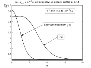
(a) $p=\frac{3}{2}$ and $N=1$

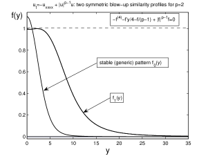
(b) $p=2$ and $N=1$

Figure 1. Two self-similar blow-up solutions of (2.3): $p=1.5$ (a) and $p=2$ (b).

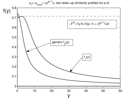
Figure 2. Two self-similar blow-up solutions of (2.3) for $p=5$.

2.2. On existence of similarity profiles for $N=1$: classification of blow-up and oscillatory bundles

We now provide extra details concerning existence of at least a single blow-up profile $f(y)$ satisfying (2.3), (2.4). We perform shooting from $y=+\infty$ by using the 2D bundle (2.18) to $y=0$, where the symmetry condition (2.4) are posed (or to $y=-\infty$, where the same bundle (2.18) with $y\mapsto-y$ takes place). By $f=f(y;C_{1},C_{2})$, we denote the corresponding solution defined on some maximal interval

(2.5) $$\textstyle{y\in(y_{0},+\infty),\quad\mbox{where}\quad y_{0}=y_{0}(C_{1},C_{2})\geq-\infty.}$$

If $y_{0}(C_{1},C_{2})=-\infty$, then the corresponding solution $f(y;C_{1},C_{2})$ is global and can represents a proper blow-up profile (but not often, see below). Otherwise:

(2.6) $$y_{0}(C_{1},C_{2})>-\infty\quad\Longrightarrow\quad f(y;C_{1},C_{2})\to\infty\quad\mbox{as}\quad y\to y_{0}^{+}.$$

Note that “oscillatory blow-up” for the ODE close to $y=y_{0}^{+}$:

(2.7) $$f^{(4)}=|f|^{p-1}f(1+o(1)),$$

where $\lim\sup f(y)=+\infty$ and $\lim\inf f(y)=-\infty$ as $y\to y_{0}^{+}$, is nonexistent. The proof is easy and follows by multiplying (2.7) by $f^{\prime}$ and integrating between two extremum points $(y_{1},y_{2})$, where the former one $y_{1}$ is chosen to be sufficiently close to the blow-up value $y_{0}^{+}$, whence the contradiction:

$$\textstyle{0<\frac{1}{2}\,(f^{\prime\prime})^{2}(y_{1})\sim-\frac{1}{p+1}\,|f|^{p+1}(y_{1})<0.}$$

We first study this set of blow-up solutions. These results are well understood for such fourth-order ODEs; see [42], so we omit some details.

Proposition 2.1.

The set of blow-up solutions $\eqref{ma3}$ is four-dimensional.

Proof. The first parameter is $y_{0}\in\mathbb{R}$. Other are obtained from the principal part of the equation (2.7) describing blow-up via (2.3) as $y\to y_{0}^{+}$. We apply a standard perturbation argument to (2.7). Omitting the $o(1)$-term and assuming that $f>0$, we find its explicit solution

(2.8) $$\textstyle{f_{0}(y)=A_{0}(y-y_{0})^{-\frac{4}{p-1}},\,\,\,A_{0}^{p-1}=\Phi(-\frac{4}{p-1}),\,\,\,\Phi(m)\equiv m(m-1)(m-2)(m-3).}$$

For convenience, the graph of $\Phi(m)$ is shown in Figure 3. Note that it is symmetric relative to $m_{0}=\frac{3}{2}$, at which $\Phi(m)$ has a local maximum:

(2.9) $$\textstyle{\Phi(\frac{3}{2})=\frac{9}{16}.}$$

Figure 3. The graph of function $\Phi(m)$ in (2.8), and towards solutions of (2.10).

By linearization, $f=f_{0}+Y$, we get Euler’s ODE:

(2.10) $$\textstyle{(y-y_{0})^{4}Y^{(4)}=pA_{0}^{p-1}\equiv p\Phi(-\frac{4}{p-1}).}$$

It follows that the general solution is composed from the polynomial ones with the following characteristic equation:

(2.11) $$\textstyle{Y(y)=(y-y_{0})^{m}\quad\Longrightarrow\quad\Phi(m)=p\Phi(-\frac{4}{p-1}).}$$

Since the multiplier $p>1$ in the last term in (2.11) and $m=-\frac{4}{p-1}$ is a solution if this “$p\times$” is omitted, this algebraic equation for $m$ admits a unique positive solution $m_{+}>3$, a negative one $m_{-}<-\frac{4}{p-1}$, which is not acceptable by (2.8), ad two complex roots $m_{1,2}$ with ${\rm Re}\,m_{1,2}=\frac{3}{2}>0$. Therefore, the general solution of (2.7) about the blow-up one (2.8), for any fixed $y_{0}$, has a 3D stable manifold. ∎

Thus, according to Proposition 2.1, the blow-up behaviour with a fixed sign (2.6) (i.e., non-oscillatory) is generic for the ODE (2.3). However, this 4D blow-up bundle together with the 2D bundle of good solutions (2.18) as $y\to\pm\infty$ are not enough to justify the shooting procedure. Indeed, by a straightforward dimensional estimate, an extra bundle at infinity is missing.

To introduce this new oscillatory bundle, we begin with the simpler ODE (2.7), without the $o(1)$-term, and present in Figure 4 the results of shooting of a “separatrix” that lies between orbits, which blow-up to $\pm\infty$. Obviously, this separatrix is a periodic solution of this equation with a potential operator. Such variational problems are known to admit periodic solutions of arbitrary period.

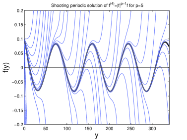
Figure 4. A periodic solution of $f^{(4)}=|f|^{p-1}f$ as a separatrix: $p=5$.

Thus, Figure 4 fixed a bounded oscillatory (periodic) solution as $y\to+\infty$. When we return to the original equation (2.3), which is not variational, we still are able to detect a more complicated oscillatory structures at $y=\infty$. Namely, these are generated by the principal terms in

(2.12) $$\textstyle{f^{(4)}=-\frac{1}{4}\,f^{\prime}y+|f|^{p-1}f+...\quad\mbox{as}\quad y\to\infty.}$$

Similar to Figure 4, in Figure 5, we present the result of shooting (from $y=-\infty$, which is the same by symmetry) of such oscillatory solutions of (2.3) for $p=5$. It is easy to see that such oscillatory solutions have increasing amplitude of their oscillations as $y\to\infty$, which, as above, is proved by multiplying (2.12) by $f^{\prime}$ and integrating over any interval $y_{1},y_{2})$ between two extrema. Figure 6 shows shooting of similar oscillatory structures at infinity for $p=7$ (a) and $p=2$ (b). It is not very difficult to prove that the set of such oscillatory orbits at infinity is 1D and this well corresponds to the periodic one in Figure 4 depending on the single parameter being its arbitrary period.

By $C_{2}^{\pm}(C_{1})$ in Figure 5, we denote the values of the second parameters $C_{2}$ such that, for a fixed $C_{1}\in\mathbb{R}$, the solutions $f(y;C_{1},C_{2}^{\pm})$ blow up to $\pm\infty$ respectively. These values are necessary for shooting the symmetry conditions (2.4).

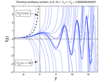
Figure 5. Shooting an oscillatory solution at infinity of (2.3): $p=5$.

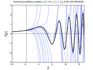
(a) $p=7$

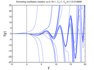
(b) $p=2$

Figure 6. Shooting an oscillatory solution at infinity of (2.3): $p=7$ (a) and $p=2$ (b).

Thus, overall, using two parameters $C_{1,2}$ in the bundle (2.18) for $y\gg 1$ leads to a well-posed problem of a 2D–2D shooting:

(2.13) $$\mbox{find $C_{1,2}$ such that:}\quad\left\{\begin{matrix}y_{0}(C_{1},C_{2})=-\infty,\quad\mbox{and}\qquad\qquad\quad\\ \mbox{no oscillatory behaviour as $y\to-\infty$}.\end{matrix}\right.$$

Concerning the actual proof of existence via shooting of at least a single blow-up patterns $f_{0}(y)$, by construction and oscillatory property of the equation (2.3), we first claim that in view of continuity relative to the parameters,

(2.14) $$\mbox{for any $C_{1}>0$, there exists $C_{2}^{*}(C_{1})\in(C_{2}^{-}(C_{1}),C_{2}^{+}(C_{1}))$ such that $f^{\prime\prime\prime}(0)=0$}.$$

We next change $C_{1}$ to prove that at this $C_{2}^{*}(C_{1})$ the derivative $f^{\prime}(0)$ also changes sign. Indeed, one can see that

(2.15) $$f^{\prime}(0;C_{1},C_{2}^{*}(C_{1}))>0\quad\mbox{for}\quad C_{1}\ll 1\quad\mbox{and}\quad f^{\prime}(0;C_{1},C_{2}^{*}(C_{1}))<0\quad\mbox{for}\quad C_{1}\gg 1.$$

Actually, this means for such essentially different values of $C_{1}$, the solution $f(y;C_{1},C_{2}^{*}(C_{1})$ has first oscillatory “humps” for $y>0$ and $y<0$ respectively. By continuity in $C_{1}$, (2.15) implies existence of a $C_{1}^{*}$ such that

(2.16) $$f^{\prime}(0;C_{1}^{*},C_{2}^{*}(C_{1}^{*}))=0,$$

which together with (2.14) induced the desired solution. Overall, the above geometric shooting well corresponds to that applied in the standard framework of classic ODE theory, so we do not treat this in greater detail. However, we must admit that proving analogously existence of the second solution $f_{0}(y)$ (detected earlier by not fully justified arguments of homotopy and branching theory and confirmed numerically) is an open problem. A more difficult open problem is to show why the problem (2.13) does not admit non-symmetric (non-even) solutions $f(y)$ (or does it?).

2.3. Dimensions $N\geq 2$: on 2D shooting and analogous nonuniqueness

In higher dimensions, it is easier to describe Type I(ss) blow-up in radial geometry, where (2.2) also becomes an ODE of the form (now $y$ stands for $|y|>0$)

(2.17) $$\textstyle{-f^{(4)}-\frac{2(N-1)}{y}\,f^{\prime\prime\prime}-\frac{(N-1)(N-3)}{y^{2}}\,f^{\prime\prime}+\frac{(N-1)(N-3)}{y^{3}}\,f^{\prime}-\frac{1}{4}\,yf^{\prime}-\frac{1}{p-1}\,f+|f|^{p-1}f=0}$$

in $\mathbb{R}$, with the same two symmetry condition (2.4). To explain the nature of difficulties in proving existence of solutions of (2.17), let us describe the admissible behaviour for $y\gg 1$. There exists a 2D bundle of such asymptotics (see details in [11, § 3.3]): as $y\to+\infty$,

(2.18) $$\textstyle{f(y)=\big{[}C_{1}y^{-\frac{4}{p-1}}+...\big{]}+\big{[}C_{2}y^{-\frac{2}{3}(N-\frac{2}{p-1})}\,{\mathrm{e}}^{-a_{0}y^{4/3}}+...\big{]},\quad\mbox{where}\quad a_{0}=3\cdot 2^{-\frac{8}{3}}}$$

and $C_{1}$ and $C_{2}$ are arbitrary parameters. This somehow reminds a typical centre manifold structure of the origin $\{f=0\}$ at $y=\infty$: the first term in (2.18) is a node bundle with algebraic decay, while the second one corresponds to “non-analytic” exponential bundle around any of algebraic curves. Thus, a dimensionally well-posed shooting is:

(2.19) Shooting:    using 2 parameters $$C_{1,2}$$ in (2.18) to satisfy 2 conditions (2.4).

In case of analytic dependence of solutions of (2.17) on parameters $C_{1,2}$ in the bundle (2.18) (this is rather plausible via standard trends of ODE theory, but difficult to prove), the problem cannot have more than a countable set of solutions. Actually, our numerics confirm that in wide parameter ranges of $p>1$ and $N\geq 1$, there exist not more than two solutions (up to other more unstable ones about the SSS; see Section 5):

(2.20) $$f_{0}(y)\,\,\,\mbox{with}\,\,\,\{C_{10}(p,N),C_{20}(p,N)\},\quad\mbox{and}\quad f_{1}(y)\,\,\,\mbox{with}\,\,\,\{C_{11}(p,N),C_{21}(p,N)\}.$$

The rest of this section is devoted to justify this.

The eventual similarity blow-up patterns can be characterized by their final time profiles: passing to the limit $t\to T^{-}$ in (2.1) and using the expansion (2.18) yields

(2.21) $$\mbox{if $C_{1}(p,N)\not=0$, then}\quad u(x,t)\to C_{1}|x|^{-\frac{4}{p-1}}\quad\mbox{as}\quad t\to T^{-}$$

uniformly on any compact subset of $\mathbb{R}^{N}\setminus\{0\}$. If $C_{1}=0$ in (2.18), i.e., $f(y)$ has an exponential decay at infinity, then the limit is different: in the sense of distributions,

(2.22) $$\textstyle{C_{1}(p,N)=0\,\Longrightarrow\,\framebox{$|u(x,t)|^{\frac{N(p-1)}{4}}\to C_{3}\delta(x),\,\,t\to T^{-};\,\,\,C_{3}=\int|f|^{\frac{N(p-1)}{4}}<\infty.$}}$$

It is very difficult to prove that (2.22) actually takes place at some $p=p_{\delta}(N)>1$ (even for $N=1$), and we will justify this numerically for some not that large dimensions $N\leq 11$.

We now start describe various similarity blow-up profiles for $N\geq 2$. As a first and analogous to $N=1$ example, in Figure 7, we construct numerically first two profiles, $f_{0}(y)$ and $f_{1}(y)$, for the three-dimensional case $N=3$ and $N=10$ for $p=2$, which look rather similar to those in Figure 1 for $N=1$.

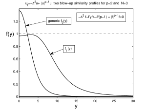
(a) $p=2,\,\,N=3$

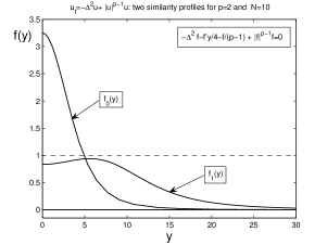
(b) $p=2,\,\,N=10$

Figure 7. Two self-similar blow-up solutions of (2.17) for $p=2$: $N=3$ (a) and $N=10$ (b).

2.4. $N\geq 2$: $p$-branches of the profile $f_{0}(y)$ and $f_{1}(y)$

Such $p$-branches of solutions are a convenient way to describe families of profiles $f_{0}(y)$ depending on the exponent $p$; cf. [30, 41]. In Figure 8, we present such a branch of $f_{0}$ for $N=4$, where (a) shows the actual smooth deformation of $f_{0}(y)$ with changing $p$, while (b) is the corresponding $p$-branch. In Figure 9, the same is done for $N=8$. Note that both Figures (b) show that $\|f\|_{\infty}=f(0)$ approaches 1 for large $p$, which is a general phenomenon for such ODEs described in [30, § 5]. Similarly, Figure 10 shows $p$-branches of the second blow-up profile $f_{1}(y)$ for $p=2$ in the cases $N=1$ (a) and $N=12$ (b) (the critical dimension, where $p_{\rm S}=2$).

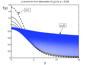
(a) $f_{0}$-deformation

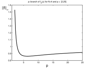
(b) $p$-branch

Figure 8. The $p$-branch of blow-up self-similar profiles $f_{0}(y)$ for $N=4$.

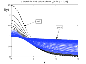
(a) $f_{0}(y)$-deformation

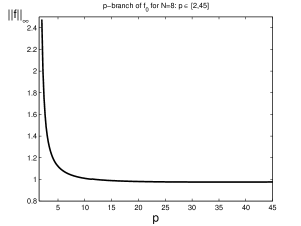
(b) $p$-branch

Figure 9. The $p$-branch of blow-up self-similar profiles $f_{0}(y)$ for $N=8$.

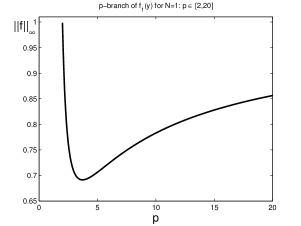
(a) $p$-branch for $N=1$

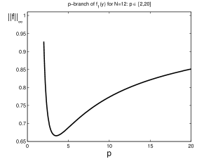
(b) $p$-branch for $N=12$

Figure 10. The $p$-branches of blow-up self-similar profiles $f_{1}(y)$ for $p=2$: $N=1$ (a) and $N=12$ (b).

It is well understood that for equations such as (2.17), the solutions $f(y)$ blow-up as $p\to 1^{+}$ with a super-exponential rate $\sim(p-1)^{-1/(p-1)}$; see [30, 41]. As an example, in Figure 11, we present such a blowing up behaviour of the $p$-branch of $f_{1}(y)$ for $N=6$.

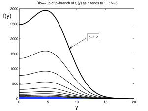
(a) $f_{1}$-deformation

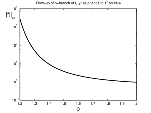
(b) $p$-branch

Figure 11. Blow-up as $p\to 1^{-}$ of the $p$-branches of profiles $f_{1}(y)$ for $N=6$: $p$-deformation of $f_{1}(y)$ (a) and blow-up of $p$-branch in the log-scale (b).

2.5. $N\geq 2$: $N$-branches of blow-up profiles

Firstly, in some $N$-intervals, there is a continuous dependence of $f_{0}(y)$ on the dimension, as Figure 12 clearly shows for $p=2$ and Figure 13 for $p=5$ (those values of $p$ will be constantly used later on for the sake of comparison).

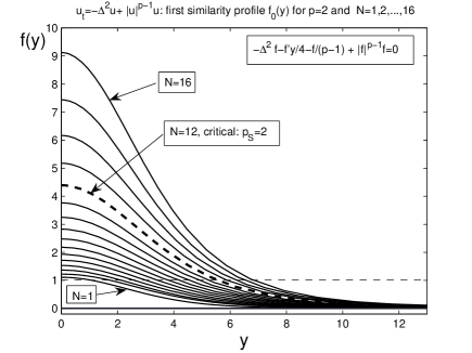
Figure 12. Similarity blow-up solutions $f_{0}(y)$ of (2.17) for $p=2$ in dimensions $N=1,\,2,\,...\,,\,16$.

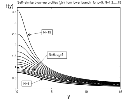
Figure 13. Similarity solutions $f_{0}$ of (2.17) for $p=5$ and $N=1,\,2,\,...\,$, $15$.

However, we found that there are other solutions of the monotone type $f_{0}$, which are shown in Figure 14 for $p=5$ (a) and $p=2$ (b), where in the latter one the profile from the lower $N$-branch is not shown as being too relatively small.

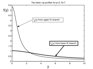
(a) $p=5$

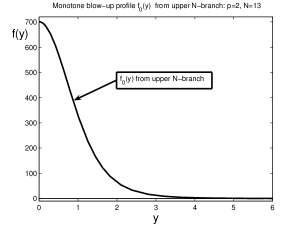
(b) $p=2$

Figure 14. Two monotone blow-up profiles of $f_{0}$-type: for $p=5$ (a) and for $p=2$ (b).

Thus, secondly, this nonuniqueness demands another approach to branching, namely, the $N$-branching that we perform next. In Figure 15, we show the lower $N$-branch of solutions $f_{0}(y)$ for $p=5$, where (a) describes the deformation of $f_{0}$ and (b) gives the actual $p$-branch. Blow-up of the upper $N$-branch as

(2.23) $$\textstyle{N\to N_{5}^{+},\quad\mbox{where}\quad N_{p}:\,\,\,\frac{N+4}{N-4}=p,}$$

so that $N_{5}=6$ for $p=5$, is shown in Figure 16, with the same meaning of (a) and (b). A general view of the whole $N$-branch of $f_{0}$ for $p=5$ is schematically explained in Figure 17, where by dotted line we draw a possible expected but still hypothetical connection of the lower (stable) and the upper (more unstable, plausibly) $f_{0}$-branches, which we were not able to reconstruct numerically. Numerical continuation in the parameter $N$ is quite a challenging problem in some $N$-ranges.

Thus we expect that there exists a saddle-node bifurcation at some

(2.24) $$p=5:\quad N_{\rm sn}\in(14.979,15).$$

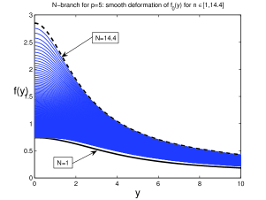
(a) $f_{0}$-deformation

(b) lower $N$-branch

Figure 15. Lower $N$-branch of $f_{0}$ for $p=5$.

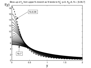
(a) $f_{0}$-deformation

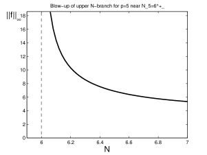
(b) upper $N$-branch

Figure 16. Upper $N$-branch of $f_{0}$ for $p=5$ with blow-up as $N\to 6^{+}$.

\psfrag{||f||}{$\|f\|_{\infty}$}\psfrag{p}{$p$}\psfrag{ff}{$\|f\|_{\infty}$}\psfrag{NN}{$N$}\psfrag{Nsn}{$N_{\rm sn}$}\psfrag{v(x,t-)}{$v(x,T^{-})$}\psfrag{final-time profile}{final-time profile}\psfrag{tapp1}{$t\approx 1^{-}$}\psfrag{x}{$x$}\psfrag{0<t1<t2<t3<t4}{$0<t_{1}<t_{2}<t_{3}<t_{4}$}\psfrag{0}{$0$}\psfrag{l}{$l$}\psfrag{-l}{$-l$}\includegraphics[scale={0.36}]{Nbrp5.eps}

Figure 17. The whole $N$-branch of $f_{0}$ for $p=5$.

In Figure 18 for $p=2$, we show blow-up of the upper $N$-branch as $N\to N_{2}=12^{+}$. We then expect that the lower and upper branches have a turning (saddle-node) bifurcation point at some

$$p=2:\quad N_{\rm sn}\in(20.3,23].$$

We hope that such an interesting saddle-node branching phenomenon will attract true experts in numerical methods, bearing in mind that numerical experiments might be for a long time the only tool of the study of such blow-up phenomena.

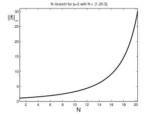
(a) lower $N$-branch

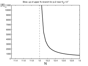
(b) upper $N$-branch

Figure 18. Lower and upper $N$-branches of $f_{0}$ for $p=2$: the lower branch for $N\in[1,20.3]$ (a) and blow-up of the upper one as $N\to 12^{+}$ (b).

Finally, in Figure 19, we present the numerical results confirming $N$-branching for $p=2$ of the second blow-up profile $f_{1}$, where, as usual, (a) describes smooth deformation of $f_{1}(y)$, while (b) shows the $N$-branch. It seems that $N$-branches of $f_{1}$ are global and do not suffer from a saddle-node bifurcations.

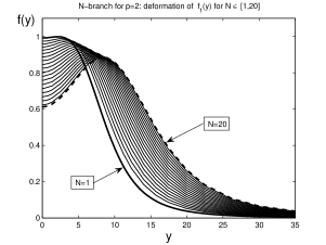
(a) $f_{0}$-deformation

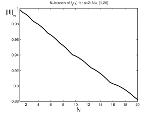
(b) $N$-branch

Figure 19. The $N$-branch of $f_{1}$ for $p=2$ and $N\in[1,20]$.

2.6. On sign changes of $f_{0}(y)$ and $f_{1}(y)$

We now study some particularly important properties of blow-up similarity profiles. We begin with the easier property of sign changes. We have seen already several strictly positive profiles $f_{0}(y)$ for some $p$’s, which is rather surprising since the equations do not obey the Maximum Principle. However, we will show that, for smaller $p$, the similarity profiles can gain extra zeros as sign changes. Such $p$’s , when a zero is gained, we denote by $p_{0}(N)$.

Consider one dimension $N=1$. Firstly, the attentive Reader can see that in Figure 1(a), already for $p=\frac{3}{2}$ the profile $f_{0}(y)$ changes sign, while for $p=2$, it is positive. Hence, $p_{0}(1)\in(\frac{3}{2},2)$. Secondly, more thorough numerics are presented in Figure 20, where (a) shows $f_{0}$’s in a vicinity of

(2.25) $$p_{0}(1)=1.7358...\,,$$

while (b) shows a sharp shooting of the critical value (2.25). Figure 21 shows shooting

$$p_{0}^{(1)}(1)=1.23...\,,$$

at which the second profile $f_{1}(y)$ gets a new zero. By the boldface line we denote a new “$p$-undetected” solution with extra zeros gained at another $p_{01}$, showing that such roots are not unique. Since $f_{1}(y)$ is expected to be less stable, we will concentrate on the roots $p_{0}$ for the generic blow-up profile $f_{0}(y)$.

Thus, similarly, Figure 22(a) yields

(2.26) $$p_{0}(3)=1.446...\quad\mbox{and}\quad p_{0}(9)=1.204...\,.$$

In Figure 23(a), a similar phenomenon is checked for $N=10$, with $p_{0}(10)=1.188...\,.$ In (b), we see no sign changes of $f_{0}(y)$ for $N=12$, but this happens for smaller $p\approx 1^{+}$, when $f(0)$ gets $10^{5}$–$10^{6}$, while their negative counterparts take values $\sim-10^{5}$, and numerics become rather unreliable. The overall numerical results for shooting $p_{0}(N)$ are shown in Table 1.

Table 1. Roots $p_{0}(N)$ for profiles $f_{0}(y)$ to get a new zero

$N$	$p_{0}(N)$
$1$	1.7358…
$2$	1.53…
$3$	1.446…
$4$	1.377…
$5$	1.320…
$6$	1.28…
$7$	1.25…
$8$	1.226…
$9$	1.204…
$10$	1.188…
$11$	1.16…

A proper asymptotic theory for $p\approx 1^{+}$ involving expansions such as (2.18) and $(p-1)^{-\frac{1}{p-1}}$-scaling of the ODE (2.17) (cf. [30, § 5]) would be fruitful. Note that we have observed some numerical evidence for existence of the second root $p_{01}$ for $N=8$ and $9$ (see the dotted line in Figure 22), which is surprising in view of non-oscillating of the exponential term in (2.18), but numerics were too difficult and rather poor to identify the new root if any.

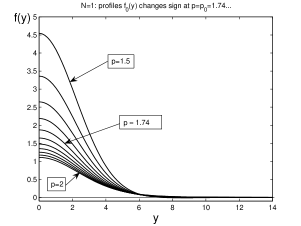
(a) $f_{0}$ profiles, $N=1$

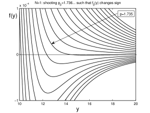
(b) shooting $p_{0}(1)$, $N=1$

Figure 20. Shooting the root $p_{0}(1)$ for $N=1$.

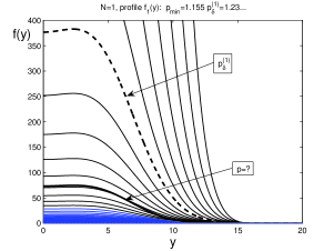
(a) $f_{1}$ profiles, $N=1$

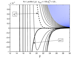
(b) shooting $p_{0}^{(1)}(1)$, $N=1$

Figure 21. Shooting the root $p_{0}^{(1)}(1)$ for $N=1$.

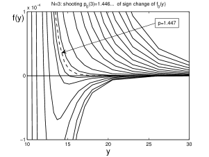
(a) shooting $p_{0}(3)$

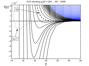
(b) $N=9$

Figure 22. Shooting the root $p_{0}(1)$: for $N=3$ (a) and for $N=9$ (b).

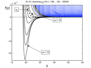
(a) shooting $p_{0}$ for $N=10$

(b) $N=12$

Figure 23. Shooting the root $p_{0}(1)$: for $N=10$ (a) and no sign changes of $f_{0}(y)$ for $N=12$ for $p\geq 1.3$ (b).

2.7. On final time measure-like Type I(ss) blow-up

This is a much more difficult problem, which we resolve numerically for $N=1$ only. For $N\geq 2$, we got no sufficiently reliable results (rather plausibly, such a self-similar phenomenon may be unavailable in some higher dimensions).

We will refine Figure 20. We claim that the equation (2.22) has the following root:

(2.27) $$p_{\delta}(1)=1.40...<p_{0}(1)=1.7358...\,,$$

at which the coefficient $C_{1}(p,N)$ vanishes, so that $f_{0}(y)$ has exponential decay at infinity. To see this, we show in Figure 24 with the scale of $10^{-20}$ how the coefficient $C_{1}(p,1)$ changes sign around (2.27):

(2.28) $$C_{1}(1.39,1)>0,\quad\mbox{while}\quad C_{1}(1.40,1)<0.$$

Non vanishing of these two profiles in smaller scaled up to $10^{-40}$ was checked in the logarithmic scale (we do not present here a number of such numerics).

Figure 24. Shooting the root (2.27) of the algebraic equation (2.22) for $N=1$.

2.8. On non-radial self-similar blow-up patterns in dimensions $N\geq 2$

This question was not studied in the literature at all and indeed is very difficult. We make a slight observation only: the performed below linearization (4.2) about the constant equilibrium in the elliptic equation (2.2) leads to the perturbed linear elliptic equation

(2.29) $$({\bf B}^{*}+I)Y+{\bf D}(Y)=0$$

(on spectral properties of ${\bf B}^{*}$, see Lemma 4.1). Then, ${\bf B}^{*}+I$ has a large unstable subspace

(2.30) $$E^{\rm u}(0)={\rm Span}\{\psi_{\beta}:\,\,\,\lambda_{\beta}+1>0\},$$

so that the corresponding eigenfunctions may characterize possible shapes of various similarity solutions (actually, this is true for $N=1$ [3]). Roughly speaking, we claim that:

(2.31) $$\framebox{$\begin{matrix}\mbox{the dimension $M(p,N)={\rm dim}\,E^{\rm u}(0)-(N+1)$ can characterize}\vskip 3.0pt plus 1.0pt minus 1.0pt\\ \mbox{the total number of blow-up similarity patterns as solutions of (\ref{2.2}).}\end{matrix}$}$$

Note that we subtract $(N+1)$-dimensions corresponding to natural instabilities relative to shifting the blow-up point $0\in\mathbb{R}^{N}$ ($N$ dimensions) and blow-up time $T$ (1 dimension). These unstable modes are not available if the blow-up point $(0,T)$ is fixed. The dimension $M=M(p,N)$ can characterize the total number of solutions $f(y)$ of the elliptic problem (2.2) including many non-radial ones. In other words, we expect that those unstable $M$ modes initiate heteroclinic connections through the corresponding unstable manifold $W^{\rm u}(0)$ to the set of steady solutions $\{f_{k}(y),\,k=1,2,...,M\}$. In Section 4, we show that stable modes from $E^{\rm s}(0)$ with $\lambda_{\beta}+1>0$ and the centre ones $E^{\rm c}(0)$ with $\lambda_{\beta}+1=0$ will lead to other “linearized” blow-up patterns, so that $\{f_{k}\}$ are “nonlinear eigenfunctions”.

Proving any part of the claim (2.31) is a difficult open problem for any $N\geq 2$. Note also that, for the second-order quasilinear counterpart (1.13) ($m>1$ is essential!), non radially symmetric self-similar blow-up patterns have been known for more than thirty years; see [56] and a survey [55] for extra details.

3. Type I(log): self-similar patterns with angular logTW swirl

This is a simple idea for producing non-radial blow-up patterns, but its consistency is quite questionable.

3.1. Nonstationary rescaling

Dealing with non-self-similar blow-up, instead of (2.1), we use the full similarity scaling:

(3.1) $$\textstyle{u(x,t)=(T-t)^{-\frac{1}{p-1}}v(y,\tau),\quad y=\frac{x}{(T-t)^{1/4}},\quad\tau=-\ln(T-t)\to+\infty,\,\,t\to T^{-}.}$$

Then $v(y,\tau)$ solves the following parabolic equation:

(3.2) $$\textstyle{v_{\tau}={\bf A}(v)\equiv-\Delta^{2}v-\frac{1}{4}\,y\cdot\nabla v-\frac{1}{p-1}\,v+|v|^{p-1}v\quad\mbox{in}\quad\mathbb{R}^{N}\times(\tau_{0},\infty),\,\,\,\tau_{0}=-\ln T,}$$

where ${\bf A}$ is the stationary elliptic operator in (2.2), so that similarity profiles (if any) are just stationary solutions of (3.2).

3.2. Blow-up angular swirling mechanism

We begin with $N=2$, where $y=(y_{1},y_{2})$, and, in the corresponding polar coordinates $\{\rho,\varphi\}$, with $\rho^{2}=y_{1}^{2}+y_{2}^{2}$,

(3.3) $$\textstyle{\Delta=\Delta_{\rho}+\frac{1}{\rho^{2}}\,D^{2}_{\varphi},\quad\mbox{where}\quad\Delta_{\rho}=D^{2}_{\rho}+\frac{1}{\rho}\,D_{\rho}\quad\mbox{and}\quad y\cdot\nabla=\rho D_{\rho}.}$$

We next consider a TW in the angular direction by fixing the angular dependence

(3.4) $$\varphi=\sigma\,\tau+\mu\equiv-\sigma\ln(T-t)+\mu,\quad\mu\in(0,2\pi),$$

where $\sigma\in\mathbb{R}$ is a constant (a nonlinear eigenvalue). In the original independent variables $\{x,t\}$, (3.4) represents a blowing up logarithmic TW in the angular direction with unknown wave speeds $\sigma$. In other words, (3.4) assumes that blowing up as $t\to T^{-}$ is accompanied by a focusing TW-angular behaviour also in a logarithmic blow-up manner.

Thus, assuming the logTW angular dependence (3.4) of the solution $v=v(y,\mu,\tau)$, $\varphi=\sigma\tau+\mu$, yields the equation

(3.5) $$\textstyle{v_{\tau}={\bf A}(v)-\sigma v_{\mu}\equiv-\Delta^{2}v-\frac{1}{4}\,y\cdot\nabla v-\frac{1}{p-1}\,v+|v|^{p-1}v-\sigma v_{\mu}\quad\mbox{in}\quad\mathbb{R}^{N}\times(\tau_{0},\infty),}$$

where $\tau_{0}=-\ln T$. In particular, this non-radial self-similar blow-up may be generated by bounded steady profiles satisfying

(3.6) $$\textstyle{{\bf A}(f)-\sigma f_{\mu}\equiv-\Delta^{2}f-\frac{1}{4}\,y\cdot\nabla f-\frac{1}{p-1}\,f+|f|^{p-1}f-\sigma f_{\mu}=0\quad\mbox{in}\quad\mathbb{R}^{2}.}$$

For $\sigma\neq 0$, which, as we have mentioned, plays the role of a nonlinear eigenvalue, the blow-up behaviour with swirl corresponds to periodic orbits as $\omega$-limit sets; see a discussion in [27] to the NSEs (1.18). As a first approach to solvability of (3.6), one can assume branching of a solution $f(\rho,\mu)$ from the radial one $f_{0}$ at $\sigma=0$. Then setting $f=f_{0}+\sigma\psi^{*}+...$ yields that $\psi^{*}(\rho,\mu)$ must be a nontrivial non-radial eigenfunction for $\lambda=0$:

(3.7) $${\bf A}^{\prime}(f_{0})\psi^{*}=0.$$

On the other hand, branches of solutions $f$ of (3.6) may occur at a saddle-node bifurcation $\sigma=\sigma_{*}\neq 0$, where $\sigma_{*}$ belongs to spectrum of the linear pencil ${\bf A}^{\prime}(f)-\sigma D_{\mu}$. Both eigenvalue problem are very difficult, and we do not exclude the possibility that, overall, the problem (3.6) for $\sigma\neq 0$ may admit such solutions only that are singular at the origin $y=0$. Anyway, even in this unfortunate case, we believe that introducing such rather unknown types of non-radial blow-up with swirl deserves mentioning among other more practical patterns. Let us also mention that, in $\mathbb{R}^{N}$, one can distribute the variables as

$$y=(y_{1},y_{2},y^{\prime})\in\mathbb{R}^{N},\quad\mbox{where}\quad y^{\prime}\in\mathbb{R}^{N-2},$$

and arrange a $\sigma_{1}$-logTW in variables $(y_{1},y_{2})$ only to get periodic blow-up behaviour. Choosing other disjoint pairs $(y_{k},y_{k+1})$ and constructing the corresponding periodic swirl in these variables, in particular, it is formally possible to produce a quasi-periodic blow-up swirl with arbitrary number $\sigma_{1}$, …, $\sigma_{n}$, $n\leq\big{[}\frac{N}{2}\big{]}$, of fundamental frequencies. Of course, this leads to complicated nonlinear eigenvalue problems, which are open even for $n=1$, i.e., for the periodic motion introduced above first.

3.3. Remark: on the origin of logTWs and invariant solutions

The scaling group-invariant nature of such logTWs seems was first obtained by Ovsiannikov in 1959 [73], who performed a full group classification of the nonlinear heat equation

$$u_{t}=(k(u)u_{x})_{x},$$

for arbitrary functions $k(u)$. In particular, such invariant solutions appear for the porous medium and fast diffusion equations for $k(u)=u^{n}$, $n\neq 0$:

$$\textstyle{u_{t}=(u^{n}u_{x})_{x}\quad\Longrightarrow\quad\exists\,\,\,u(x,t)=t^{-\frac{1}{n}}f(x+\sigma\ln t),\quad\mbox{where}\quad-\frac{1}{n}\,f+\sigma f^{\prime}=(f^{n}f^{\prime})^{\prime}.}$$

Blow-up angular dependence as $t\to T^{-}$ such as in (3.4) was studied later on in [1], where the corresponding similarity solutions for the reaction-diffusion equation with source (1.13) in $\mathbb{R}^{2}\times(0,T)$ were indicated by reducing the PDE to a quasilinear elliptic problem (it seems, there is no still a rigorous proof of existence of such patterns). For parabolic models such as (1.13), that are order-preserving via the MP and do not have a natural “vorticity” mechanism, such “spiral waves” as $t\to T^{-}$ must be generated by large enough initial data specially “rotationally” distributed in $\mathbb{R}^{2}$. For the biharmonic operator as in (1.1) with no MP, such a swirl blow-up dependence may be more relevant; see below.

4. Type I(Her): non self-similar “linearized” patterns with a local generalized Hermite polynomial structure

For the classic R–D equation (1.7), a countable set of non self-similar blow-up patterns of a similar structure was first formally introduced in [84], though the history of such non-self-similar blow-up asymptotics goes back to Hocking–Stuartson–Stuart in 1972, [50], who invented an interesting novel formal technique of analytic expansions (in fact, an analogy of a centre manifold analysis) to confirm that blow-up occurs on subsets governed by the “hot spot” variables, as $t\to T^{-}$:

(4.1) $$\textstyle{u(x,t)=(T-t)^{-\frac{1}{p-1}}\,\big{[}f_{*}(\xi)+o(1)\big{]},\quad\mbox{where}\quad\xi=\frac{x}{\sqrt{(T-t)|\ln(T-t)|}}}$$

and $f_{*}$ is a unique solutions of a Hamilton-Jacobi equation of the form (4.15) (with $\frac{1}{4}\mapsto\frac{1}{2}$). A justified construction of such patterns and other applications were performed a few years later mainly in dozens of papers by Herrero and Velázquez; see [47, 83] as a guide together with other papers traced by the MathSciNet. It is curious that earlier, in 1987, a sharp upper bound of such a non-similarity blow-up evolution (4.1) (“first half of blow-up”) was proved in [36] by a modification of Friedman–McLeod gradient estimate [17], though the “second half of blow-up” took extra ten years co complete along similar lines, [18, § 7].

For the RDE–4, there is no hope to get an easy and fast rigorous justification of such non-self-similar blow-up scenario, though the main idea remains the same. We follow [19] and also [20], where such a construction applied to non-singular absorption phenomena (regular flows with no blow-up), so a full mathematical justification is available therein.

4.1. Linearization and spectral properties

The construction of such blow-up patterns is as follows. Performing the standard linearization about the constant equilibrium in the equation (3.2) yields the following perturbed equation:

(4.2) $$\textstyle{v=f_{*}+Y,\,\,f_{*}=(p-1)^{-\frac{1}{p-1}}\quad\Longrightarrow\quad Y_{\tau}=({\bf B}^{*}+I)Y+{\bf D}(Y),}$$

where ${\bf D}(Y)=c_{0}Y^{2}+...$, $c_{0}=\frac{p}{2}(p-1)^{\frac{1}{p-1}}$, is a quadratic perturbation as $Y\to 0$ and

(4.3) $$\textstyle{{\bf B}^{*}=-\Delta^{2}-\frac{1}{4}\,y\cdot\nabla\quad\mbox{in}\quad L^{2}_{\rho^{*}}(\mathbb{R}^{N}),\,\,\,\rho^{*}(y)={\mathrm{e}}^{-a|y|^{4/3}},\quad a\in\big{(}0,3\cdot 2^{-\frac{8}{3}}\big{)},}$$

is the adjoint Hermite operator with some good spectral properties [9]:

Lemma 4.1.

${\bf B}^{*}:H^{4}_{\rho^{*}}(\mathbb{R}^{N})\to L^{2}_{\rho^{*}}(\mathbb{R}^{N})$ is a bounded linear operator with the spectrum

(4.4) $$\textstyle{\sigma({\bf B}^{*})=\{\lambda_{\beta}=-\frac{|\beta|}{4},\,\,\,|\beta|=0,1,2,...\}\quad\big{(}=\sigma({\bf B}),\,\,{\bf B}=-\Delta^{2}+\frac{1}{4}\,y\cdot\nabla+\frac{N}{4}\,I\big{)}.}$$

Eigenfunctions $\psi_{\beta}^{*}(y)$ are $|\beta|$th-order generalized Hermite polynomials:

(4.5) $$\textstyle{\psi_{\beta}^{*}(y)=\frac{1}{\sqrt{\beta!}}\big{[}y^{\beta}+\sum_{j=1}^{[|\beta|/4]}\frac{1}{j!}(\Delta)^{2j}y^{\beta}\big{]},\quad|\beta|=0,1,2,...\,,}$$

and the subset $\{\psi_{\beta}^{*}\}$ is complete in $L^{2}_{\rho^{*}}(\mathbb{R}^{N})$.

As usual, if $\{\psi_{\beta}\}$ is the adjoint basis of eigenfunctions of the adjoint operator

(4.6) $$\textstyle{{\bf B}=-\Delta^{2}+\frac{1}{4}\,y\cdot\nabla+\frac{N}{4}\,I\quad\mbox{in}\quad L^{2}_{\rho}(\mathbb{R}^{N}),\quad\mbox{with}\quad\rho=\frac{1}{\rho^{*}},}$$

with the same spectrum (4.4), the bi-orthonormality condition holds in $L^{2}(\mathbb{R}^{N})$:

(4.7) $$\langle\psi_{\mu},\psi_{\nu}^{*}\rangle=\delta_{\mu\nu}\quad\mbox{for any}\quad\mu,\,\,\nu.$$

4.2. Inner expansion

Thus, in the Inner Region characterized by compact subsets in the similarity variable $y$, we assume a centre or a stable subspace behaviour as $\tau\to+\infty$ for the linearized operator ${\bf B}^{*}+I$:

(4.8) $$\begin{matrix}\mbox{centre:}\quad Y(y,\tau)=a(\tau)\psi_{\beta}^{*}(y)+w^{\bot}\quad(\lambda_{\beta}=-1,\,\,|\beta|=4),\quad\,\,\vskip 3.0pt plus 1.0pt minus 1.0pt\vskip 3.0pt plus 1.0pt minus 1.0pt\\ \mbox{stable:}\quad Y(y,\tau)=-C{\mathrm{e}}^{\lambda_{\beta}\tau}\psi_{\beta}^{*}(y)+w^{\bot}\quad(\lambda_{\beta}<-1,\,\,|\beta|>4).\end{matrix}$$

For the centre subspace behaviour in (4.8), substituting the eigenfunctions expansion into equation (4.2) yields the following coefficient:

(4.9) $$\textstyle{\dot{a}=a^{2}\gamma_{0}+...,\quad\mbox{where}\quad\gamma_{0}=c_{0}\langle(\psi_{\beta}^{*})^{2},\psi_{\beta}\rangle\quad\Longrightarrow\quad a(\tau)=-\frac{1}{\gamma_{0}\,\tau}+...\,.}$$

Note that for the matching purposes, we have to assume that (see details in [19]):

(4.10) $$\mbox{if $\psi_{\beta}^{*}(0)>0$, then}\quad\gamma_{0}>0\quad\mbox{and}\quad C>0.$$

Actually, for $k=4$ and $N=1$, it is calculated explicitly that

(4.11) $$\textstyle{\gamma_{0}=-c_{0}136\sqrt{6}<0,}$$

so that the centre manifold patterns with the positive eigenfunction

(4.12) $$\textstyle{\psi_{4}^{*}(y)=\frac{1}{\sqrt{24}}\,(y^{4}+24)}$$

correspond to solutions that blow-up on finite interfaces; see [40, § 3]. A full justification of such a behaviour can be done along the lines of classic invariant manifold theory (see e.g. [60]), though can be very difficult.

Actually, we can construct more general asymptotics by taking an arbitrary linear combination of eigenfunctions from the centre subspace. Overall, the whole variety of such asymptotics is characterized as follows:

(4.13) $$Y(y,\tau)=a(\tau)|y|^{\beta}\chi(\varphi)+...\,,\quad\mbox{where}\quad a(\tau)=-\left\{\begin{matrix}\,\,\,\frac{1}{\gamma_{0}\tau}+...\,\,\,\quad\mbox{for}\quad|\beta|=4,\vskip 3.0pt plus 1.0pt minus 1.0pt\\ C{\mathrm{e}}^{\lambda_{\beta}\tau}+...\quad\mbox{for}\quad|\beta|>4.\end{matrix}\right.$$

In general, here, $\chi(\varphi)>0$ is an arbitrary smooth function on the sphere ${\mathbb{S}}^{N-1}$, where its positivity is induced by matching issues to be revealed below.

4.3. Outer region: matching

We follow [19], where it is shown that the asymptotics (4.8) admit matching with the Outer Region, being a Hamilton–Jacobi (H–J) one. More precisely, in the centre case with $|\beta|=4$, according to (4.8), (4.9), we introduce the outer variable and obtain from (3.2) the following perturbed H–J equation:

(4.14) $$\textstyle{\xi=\frac{y}{\tau^{1/4}}\quad\Longrightarrow\quad v_{\tau}=-\frac{1}{4}\,\xi\cdot\nabla v-\frac{1}{p-1}\,v+|v|^{p-1}v+\frac{1}{\tau}\,\big{(}\frac{1}{4}\,\xi\cdot\nabla v-\Delta^{2}v\big{)}.}$$

Passing to the limit as $\tau\to+\infty$ in such singularly perturbed PDEs is not easy at all even in the second-order case (see a number of various applications in [39]). Though currently not rigorously (this looks being completely illusive), we assume stabilization to the stationary solutions $f(\xi)$ satisfying the unperturbed H–J equation:

(4.15) $$\textstyle{-\frac{1}{4}\,\xi\cdot\nabla f-\frac{1}{p-1}\,f+|f|^{p-1}f=0\quad\mbox{in}\quad\mathbb{R}^{N}.}$$

This is solved via characteristics, where we have to choose the solution satisfying (4.13):

(4.16) $$\textstyle{f(\xi)=f_{*}-\frac{1}{\gamma_{0}}\,|\xi|^{4}\,\chi(\varphi)+...\quad\mbox{as}\quad\xi\to 0\quad\Longrightarrow\quad f(\xi)=f_{*}(1+c_{*}|\xi|^{4}\chi(\varphi))^{-\frac{1}{p-1}},}$$

where $c_{*}=\frac{1}{\gamma_{0}}\,(p-1)^{p/(p-1)}$. Since $\gamma_{0}<0$ according to (4.11), the resulting profile satisfies $f(\xi)\geq f_{*}$ and blows up on the surface $\{c_{*}|\xi|^{4}\chi(\varphi)=-1\}$. Note that this actual nonexistence of a bounded centre subspace pattern plus the known unstable eigenspace of ${\bf B}^{*}+I$ in the linearized equation (4.2) somehow reflect existence of two self-similar solutions $f_{0}(y)$ and $f_{1}(y)$ as “nonlinear eigenfunctions”; see [40].

Thus, these centre subspace patterns are not bounded and should be excluded from the consideration. On the other hand, for the $2m$th-order PDE (1.17) with odd $m=3,5,...\,$, we have $\gamma_{0}>0$ and then (4.16) can represent standard blow-up patterns, [19].

Similarly, for the stable behaviour for $|\beta|>4$ in (4.8), we use the following change:

(4.17) $$\textstyle{\xi={\mathrm{e}}^{\frac{4-|\beta|}{4|\beta|}\,\tau}\,y\quad\Longrightarrow\quad v_{\tau}=-\frac{1}{|\beta|}\,\xi\cdot\nabla v-\frac{1}{p-1}\,v+|v|^{p-1}v-{\mathrm{e}}^{-\frac{|\beta|-4}{|\beta|}\,\tau}\,\Delta^{2}v.}$$

Passage to the limit $\tau\to+\infty$ and matching with Inner Region are analogous and lead to truly existent blow-up patterns for any $m\geq 2$ in (1.17), [19].

Overall, according to matching conditions (4.13) and (4.17), the whole set of possible blow-up patterns of Type II(Her) is composed from a countable set for $|\beta|=4$ ($m$ odd), 5, 6, … of continuous (uncountable) families induced by smooth functions $\chi$ on ${\mathbb{S}}^{N-1}$.

5. Type II(sing): linearization about the SSS and matching

The idea of such Type II blow-up patterns for the RDE–2 (1.7) is due to Herrero–Velázquez [49], where a justification of existence was achieved (see [69] for extra details). We apply this method to the RDE–4 (1.1) and, by the same reasons, we are not obliged to concentrate on a proof. Thus, instead of the linearization (4.2) about the constant equilibrium, we perform it about a singular one.

5.1. Singular stationary solution (SSS)

Consider the stationary equation

(5.1) $$-\Delta^{2}U+|U|^{p-1}U=0\quad\mbox{in}\quad\mathbb{R}^{N}\setminus\{0\}.$$

The explicit radial SSS has the standard scaling invariant form

(5.2) $$\begin{matrix}U(y)=C_{*}\,|y|^{-\mu},\quad\mbox{where}\quad\mu=\frac{4}{p-1},\quad C_{*}=D^{\frac{1}{p-1}},\vskip 3.0pt plus 1.0pt minus 1.0pt\vskip 3.0pt plus 1.0pt minus 1.0pt\\ \mbox{and}\quad D=\mu(\mu+2)[(\mu+1)(\mu+3)+(N-1)(N-5-2\mu)].\end{matrix}$$

It follows that such SSS exists, i.e., $D>0$, in the following parameter ranges:

(5.3) $$\textstyle{p>\frac{N}{N-4},\,\,\,N>4,\quad\mbox{or}\quad p<\frac{N+2}{N-2},\,\,\,N>2.}$$

5.2. Linearization in Inner Region: discrete spectrum by Hardy–Rellich inequality

Thus, we perform linearization in (3.2) about the SSS:

(5.4) $$\textstyle{v=U+Y\quad\Longrightarrow\quad v_{\tau}=\hat{\bf B}^{*}Y+{\bf D}(Y),}$$

where, as usual, ${\bf D}(Y)$ is a quadratic perturbation as $Y\to 0$ and

(5.5) $$\textstyle{\hat{\bf B}^{*}={\bf H}^{*}-\frac{1}{4}\,y\cdot\nabla-\frac{1}{p-1}\,I\quad\mbox{and}\quad{\bf H}^{*}=-\Delta^{2}+\frac{pD}{|y|^{4}}\,I.}$$

Similar to Lemma 4.1, the operator $\hat{\bf B}^{*}$ at infinity admits a proper functional setting in the same metric of $L^{2}_{\rho^{*}}$. However, it is also singular at the origin $y=0$, where its setting depends on the principal part ${\bf H}^{*}$.

Proposition 5.1.

The symmetric operator ${\bf H}^{*}$ admits a Friedrich’s self-adjoint extension with the domain $H^{4}_{0}(B_{1})$, discrete spectrum, and compact resolvent in $L^{2}(B_{1})$, where $B_{1}\subset\mathbb{R}^{N}$ is the unit ball, iff

(5.6) $$\textstyle{pD\leq c_{\rm H}=\frac{[N(N-4)]^{2}}{16}.}$$

Proof. Indeed, (5.6) is just a corollary of the classic Hardy–Rellich-type inequality

(5.7) $$\textstyle{\frac{[N(N-4)]^{2}}{16}\int\limits_{B_{1}}\frac{u^{2}}{|y|^{4}}\leq\int\limits_{B_{1}}|\Delta u|^{2}\quad\mbox{for}\quad u\in H^{2}_{0}(B_{1}),}$$

where the constant is sharp. For compact embedding of the corresponding spaces, see Maz’ya [62, p. 65, etc.]. ∎

The necessary inequality (5.6) takes the form

(5.8) $$\begin{matrix}G_{p}(N)\equiv\frac{[N(N-4)]^{2}}{16}-\frac{4p}{p-1}\big{(}2+\frac{4}{p-1}\big{)}\qquad\qquad\qquad\qquad\qquad\,\,\vskip 3.0pt plus 1.0pt minus 1.0pt\vskip 3.0pt plus 1.0pt minus 1.0pt\\ \times\big{[}\big{(}1+\frac{4}{p-1}\big{)}\big{(}3+\frac{4}{p-1}\big{)}+(N-1)(N-5-\frac{8}{p-1}\big{)}\big{]}\geq 0\end{matrix}$$

and does not admit an easy analytic analysis. In Figure 25, numerics show that

(5.9) (5.8) holds for $$N\geq 24 p=2 N\geq 19 p=3$$ if , and if .

In particular, checking (5.8) at $p=+\infty$ yields the inequality:

(5.10) $$\textstyle{G_{\infty}(N)\equiv\frac{[N(N-4)]^{2}}{16}-8[3+(N-1)(N-5)]>0.}$$

If this is true, then (5.8) holds for all $p\gg 1$, so:

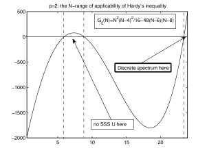
(a) $p=2$

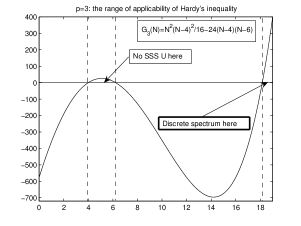
(b) $p=3$

Figure 25. Checking inequality (5.8): $p=2$ (a) and $p=3$ (b).

Proposition 5.2.

For any $N\geq 13$, there exists a $p_{\rm H}(N)>1$ such that

(5.11) $$\mbox{$(\ref{5.8})$ holds for all $p\geq p_{\rm H}(N)$},$$

and hence the operator $\hat{\bf B}^{*}$ in $(\ref{5.5})$ has a discrete spectrum in $L^{2}_{\rho^{*}}(\mathbb{R}^{N})$.

5.3. Inner Region I

Thus, we assume that, under certain conditions, (5.11) holds and $\sigma(\hat{\bf B}^{*})=\{\hat{\lambda}_{k}\}$ is discrete, with the eigenfunctions $\{\hat{\psi}^{*}_{\beta},\,|\beta|=k\}$. Furthermore, it is also convenient to assume that the spectrum is (at least partially) real. To justify such an assumption for this non-self-adjoint operator, we rewrite (5.5) in the form

(5.12) $$\textstyle{\hat{\bf B}^{*}={\bf B}^{*}+\frac{c}{|y|^{4}}\,I-\frac{1}{p-1}\,I,\quad\mbox{where}\quad c=pD}$$

and ${\bf B}^{*}$ is the previous operator (4.3) with the real spectrum shown in Lemma 4.1 (actually, this means that ${\bf B}^{*}$ admits a natural self-adjoint representation in the space $l^{2}_{\rho^{*}}$ of sequences, where it is also sectorial, [25]). Therefore, the real spectrum of (5.12) can be obtained by branching-perturbation theory (see Kato [54]) from that $\{\lambda_{\beta}=-\frac{k}{4}-\frac{1}{p-1},\,k=|\beta|\geq 0\}$ of ${\bf B}^{*}-\frac{1}{p-1}\,I$ at $c=0$. Next, the branch must be extended to $c=pD$, which is also a difficult mathematical problem; see [31, § 6] for some extra details, which are not necessary here in such a formal blow-up analysis.

Thus, we fix a certain exponentially decaying pattern in Inner Region I:

(5.13) $$Y(y,\tau)=C{\mathrm{e}}^{\hat{\lambda}_{\beta}\tau}\hat{\psi}_{\beta}^{*}(y)+...\quad\mbox{as}\quad\tau\to+\infty\quad(\hat{\lambda}_{\beta}<0).$$

If there exists $\hat{\lambda}=0\in\sigma(\hat{\bf B}^{*})$, the expansion will mimic that in (4.8) for the centre subspace case. Note that (5.13) includes all the non-radial linearized blow-up patterns.

5.4. Matching with Inner Region II close to the origin

In order to match (5.13) with a smooth bounded flow close to $y=0$, which we call Inner Region II, one needs the behaviour of the eigenfunction $\hat{\psi}_{\beta}^{*}(y)$ as $y\to 0$. To get this, without loss of generality, we assume the radial geometry. Then, the principal operator in the eigenvalue problem

(5.14) $$\textstyle{{\bf H}^{*}\hat{\psi}^{*}+...=\lambda\hat{\psi}^{*}\quad\mbox{as}\quad y\to 0}$$

yields the following characteristic polynomial (see [23]):

(5.15) $$\hat{\psi}^{*}(y)=|y|^{\gamma}+...\quad\Longrightarrow\quad H_{c}(\gamma)=-\gamma(\gamma-2)(\gamma+N-2)(\gamma+N-4)+c=0.$$

Consider the most interesting critical and extremal case

(5.16) $$\textstyle{c\equiv pD=c_{\rm H}=\frac{[N(N-4)]^{2}}{16}\quad\Longrightarrow\quad H_{c}(\gamma)\equiv-[\gamma+\mbox{$\frac{(N-4)}{2}$}]^{2}\big{[}\gamma^{2}+(N-4)\gamma-\mbox{$\frac{N^{2}}{4}$}\big{]}.}$$

There exists the double root $\gamma_{1,2}=-\frac{N-4}{2}<0,$ which generates two $L^{2}$-behaviours:

(5.17) $$\hat{\psi}_{1}^{*}(y)=|y|^{-\frac{N-4}{2}}\ln|y|(1+o(1))\quad\mbox{and}\quad\hat{\psi}_{2}^{*}(y)=|y|^{-\frac{N-4}{2}}(1+o(1))\quad\mbox{as}\,\,\,y\to 0.$$

Note that $H^{2}_{0}$-approximations of $\hat{\psi}_{2}^{*}$ establish that $c_{\rm H}$ is the best constant in (5.6). Other two roots of the characteristic equation in (5.16) are

(5.18) $$\gamma_{3,4}=\mbox{$\frac{1}{2}$}\,\big{[}\,4-N\mp\sqrt{(N-4)^{2}+N^{2}}\,\big{]},$$

where $\gamma_{3}<\gamma_{1,2}<0$ and $\gamma_{4}>0$ corresponds to $L^{2}$-solutions. We have

(5.19) $$\hat{\psi}_{3}^{*}(y)=|y|^{\gamma_{3}}(1+o(1))\not\in L^{2},$$

so that in $L^{2}$ the deficiency indices of ${\bf B}$ are $(3,3)$ and cannot be equal to $(4,4)$. Unlike the second-order case, the straightforward conclusion on the discreteness of the spectrum in the case $(4,4)$ [70, p. 90] does not apply, so Friedrich’s extension of ${\bf H}^{*}$ is constructed by other arguments [23] and include settings, where two most singular behaviour in (5.17) and (5.19) are excluded.

Overall, this gives the following behaviour of the proper eigenfunctions at the origin:

(5.20) $$\textstyle{\hat{\psi}_{\beta}^{*}(y)=-\nu_{\beta}|y|^{-\frac{N-4}{2}}+...\quad\mbox{as}\quad y\to 0\quad(\nu_{\beta}>0\,\,\,\mbox{are normalization constants}).}$$

This allows to detect the rate of blow-up of such patterns by estimating the maximal value of the expansion near the origin:

(5.21) $$\textstyle{v_{\beta}(y,\tau)=C_{*}|y|^{-\frac{4}{p-1}}-\nu_{\beta}C{\mathrm{e}}^{\hat{\lambda}_{\beta}\tau}|y|^{-\frac{N-4}{2}}+...\quad\mbox{as}\quad y\to 0\quad\mbox{and}\quad\tau\to+\infty,}$$

where we observe the natural condition of matching:

(5.22) $$\nu_{\beta}C>0.$$

Calculating the absolute maximum in $y$ of the function on the right-hand side of (5.22) (this is a standard and justified trick in some R–D problems; see e.g., [8]) yields an exponential divergence:

(5.23) $$\textstyle{\|v_{\beta}(\cdot,\tau)\|_{\infty}=d_{\beta}{\mathrm{e}}^{\rho_{\beta}\tau}+...\,,\quad\mbox{where}\quad\rho_{\beta}=\frac{8|\hat{\lambda}_{\beta}|}{(N-4)(p-p_{\rm S})}>0\quad\big{(}p>p_{\rm S}\big{)},}$$

where $d_{\beta}>0$ are some constants. Note that, depending on the spectrum $\{\hat{\lambda}_{\beta}<0\}$, (5.23) can determines a countable set of various Type II blow-up asymptotics.

Let us define more clearly the necessary matching procedure. In a standard manner, we return to the original rescaled equation (3.2) and perform the rescaling in Region II according to (5.23):

(5.24) $$\textstyle{v(y,\tau)={\mathrm{e}}^{\rho_{\beta}\tau}w(\xi,s),\quad\xi={\mathrm{e}}^{\mu_{\beta}\tau}y,\quad\mu_{\beta}=\frac{(p-1)\rho_{\beta}}{4},\quad s=\frac{1}{(p-1)\rho_{\beta}}\,{\mathrm{e}}^{(p-1)\rho_{\beta}\tau}.}$$

Then $w$ solves the following exponentially perturbed uniformly parabolic equation:

(5.25) $$\textstyle{w_{s}=-\Delta^{2}w+|w|^{p-1}w-\frac{1}{(p-1)\rho_{\beta}}\,\frac{1}{s}\,\big{[}\big{(}\frac{1}{4}+\mu_{\beta}\big{)}\xi\cdot\nabla w+\big{(}\frac{1}{p-1}+\rho_{\beta}\big{)}w\big{]}.}$$

As above, we arrive at a stabilization problem to a bounded stationary solution, which is widely used in blow-up applications (see examples in [39]). In general, once the uniform boundedness of the orbit $\{w(s),\,\,s>0\}$ is established, the passage to the limit in (5.25) as $s\to+\infty$ is a standard issue of asymptotic parabolic theory.

Our blow-up patterns correspond to the stabilization uniformly on compact subsets:

(5.26) $$w(\xi,s)\to W(\xi),\,\,s\to+\infty,\,\,\mbox{where}\,\,-\Delta^{2}W+|W|^{p-1}W=0,\,\,\xi\in\mathbb{R}^{N},\,\,W(0)=d_{\beta},$$

for all admissible $|\beta|=0,1,2,...\,$. We next discuss a crucial issue on such a matching.

5.5. Matching: on necessary structure of global bounded stationary solutions

There are two issues associated with the stationary problem (5.26).

1. Firstly and elementary, one can see that, bearing in mind the matching of Regions I and II, the bounded stationary solutions $W(\xi)$ defined by (5.26) must be positive and non-oscillatory as $\xi\to\infty$. Otherwise, such a matching with positive SSS $U(\xi)$ is impossible. There exists a definite negative result in the subcritical Sobolev range (there is a diverse literature on this popular nowadays subject, so we refer to a recent paper [45] as a guide):

(5.27) a solution $$W>0 p\in(1,p_{\rm S})$$ of (5.26) is nonexistent for .

Actually, this means that all the entire (i.e., without singularities) solutions of (5.26) are oscillatory, as Figure 26 shows for $p=2$, $N=3$. Note that we are restricted by (5.6).

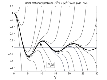
Figure 26. Shooting an oscillatory solution of (5.26) for $p=2$ and $N=3$.

2. Secondly and fortunately, existence of such positive solutions $W(\xi)$ is well established already [42, p. 908]:

(5.28) for $$p>p_{\rm S} d_{\beta}>0 W(\xi)$$, for any , there exists a unique positive solution .

Here we exclude the critical case $p=p_{\rm S}$, where exact positive solutions exist to be used in Section 6. As a numerical illustration, Figure 27 shows two such results for $N=13$ (a), where the dotted line denotes the explicit solution for $N=12$. It is clearly seen that $W(\xi)$ for $N=13$ lies above this, so remains positive. In (b), we show the positivity of the solution $W$ for $N=24$, where by (5.9), the spectrum is guaranteed to be discrete.

3. Of course, the above is not sufficient for matching of Inner Regions I and II to get a blow-up pattern. More importantly, we have the following:

Proposition 5.3.

The entire solutions $W(\xi)$ of the radial ODE $\eqref{5.22}$ are not oscillatory as $y\to+\infty$ about the SSS $(\ref{5.2})$ iff $(\ref{5.10})$ holds, and then:

(5.29) $$p\geq p_{\rm H}:\quad\mbox{$W(\xi)$ has at most finite intersections with $U(\xi)$ on $\xi\in(0,+\infty)$}.$$

Proof. It suffices to observe that, as customary, the oscillatory behaviour as $y\to+\infty$ is governed by the linearized operator therein, which is (5.5) (the limit (5.31) below justifies the linearization). Hence, in the critical Hardy case, the characteristic polynomial (5.16) has real roots only (actually, all of them, and this is quite a general property [23, 24]), and obviously the same holds in the subcritical range $pD<c_{\rm H}$, meaning that $W(\xi)$ is not oscillatory about $U(\xi)$ as $\xi\to+\infty$. Clearly, if $pD>c_{\rm H}$, (5.15) and (5.16) imply existence of a proper root $\gamma\in{\mathbb{C}}$ with a not that large negative real part. ∎

Thus, we have concluded that, for the present problem:

(5.30) discrete spectrum and non-oscillation occur in the same range $$p\geq p_{\rm H}(N)$$.

Indeed, this has some natural roots in general spectral theory of ordinary differential operators. For instance, for second-order singular operators, the non-oscillating behaviour at singular endpoints always imply existence of a self-adjoint extension in $L^{2}$ with a discrete spectrum; see Lemma 3.1.1 in [58, p. 74]. For higher-order symmetric operators [70], such a universal conclusion is not that clear, though is easily observed in particular problems related to simpler homogeneous operators for Hardy’s inequalities as in [23, 24].

Proposition 5.3 for $p>p_{\rm H}(N)$ was proved in [42, p. 909], where other important properties of entire solutions $W(\xi)$ of (5.26) have been established. So we do not need to mention them here in detail and will use the following only (see also [7]):

(5.31) $$\textstyle{\big{(}\frac{p+1}{2}\big{)}^{\frac{1}{p-1}}>\frac{W(\xi)}{U(\xi)}\to 1\quad\mbox{as}\quad\xi\to+\infty.}$$

However, a number of problems concerning (5.2) remain open. For instance, proving that (cf. Open Problem 3 in [42, p. 915] on ordering of the family $\{W(\xi),\,d_{\beta}>0\}$)

(5.32) for $$p\geq p_{\rm H}(N) W(\xi) U(\xi)$$, does not intersect .

Note that in view of inevitable using shooting techniques, the property (5.32) is very difficult to check numerically.

Fortunately, as a standard topology suggests, solving the open problem (5.32) is not necessary for the validity of the matching of Inner Regions I and II, since the non-oscillating of $W(\xi)$ as $\xi\to+\infty$ is in principal demand (one can see that existence of a finite number of intersections cannot spoil matching). Thus, we conclude that:

(5.33) for $$p\geq p_{\rm H}(N)$$, matching of two flows (5.13) and (5.26) is plausible,

though a huge mathematical work is necessary to prove this (the author still believes that this can be done in a reasonably finite period of time, but its scale can be beyond any expectation).

5.6. On new blow-up similarity solutions in the oscillatory range $p<p_{\rm H}$

Thus, (5.16) clearly shows that for $p<p_{\rm H}$ the solutions $W(\xi)$ are oscillatory about the SSS $U(\xi)$. Such topology (as in the second-order case, see [38] and later publications) suggests that in this subcritical Hardy range there may be a sequence of similarity profiles satisfying (2.17) and exhibiting arbitrary finite oscillations about $U(\xi)$ for sufficiently small radial $\xi>0$. Such self-similar blow-up profiles concentrated in a neighbourhood of the unstable singular equilibrium $U$ (above $U$, a.a. solutions must blow-up), are expected to be also highly unstable, at least in comparison with the previous profiles $f_{0}$ and $f_{1}$ studied in Section 2. Therefore, we ignore such new families (possibly countable depending on parameter ranges) of the s-s blow-up.

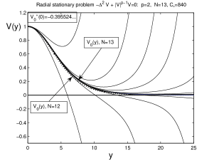
(a) $N=13>12=N_{2}$

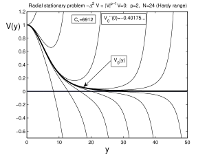
(b) $N=24$

Figure 27. Checking the positivity of the solutions of (5.26) for $p=2$: $N=13$ (a) and $N=24$ (b).

5.7. On related non-radial blow-up patterns

These can be predicted in a various ways. Firstly, one can start with a non-radial SSS solving the elliptic equation (5.1), but surely such ones are unknown. Secondly, under the condition (5.6), a non-radial eigenfunction $\psi_{\beta}^{*}(y)$ (e.g., corresponding to an “angular” swirl obtained by angular separation of variables) of $\hat{\bf B}^{*}$ can be taken into account. Then matching will assume using non-radial entire solutions of (5.13), which then deserves further study.

6. Type I(LN): non self-similar blow-up evolution on a manifold of generalized Loewner–Nirenberg stationary solutions

6.1. Classic Loewner–Nirenberg (L–N) conformally invariant exact solutions

These are classic solutions obtained in Loewner–Nirenberg [59] in 1974 for the second-order elliptic equation

(6.1) $$\textstyle{\Delta W+W^{p}=0\quad\mbox{in}\quad\mathbb{R}^{N},\,\,\,W(0)=d>0,\quad\mbox{for}\quad p=p_{\rm S}=\frac{N+2}{N-2}\quad(N>2),}$$

which are invariant under conformal and projective transformations (symmetries of (6.1) were earlier studied by Ibragimov in 1968 [51]). These solutions are given by

(6.2) $$\textstyle{W_{0}(\xi)=d\,\Big{[}\frac{N(N-2)}{N(N-2)+d^{4/(N-2)}|\xi|^{2}}\Big{]}^{\frac{N-2}{2}}>0\quad\mbox{in}\quad\mathbb{R}^{N}}$$

and exhibit a number of uniqueness and other exceptional properties of the equation (6.1).

6.2. Generalized L–N solutions for the biharmonic equation

For the critical biharmonic counterpart of (6.1)

(6.3) $$\textstyle{-\Delta^{2}W+|W|^{p-1}W=0\quad\mbox{in}\quad\mathbb{R}^{N},\,\,\,W(0)=d>0;\,\,\,p=p_{\rm S}=\frac{N+4}{N-4}\quad(N>4),}$$

the corresponding exact solutions are known from the 1980s at least, which we call the generalized L–N ones:

(6.4) $$\textstyle{W_{0}(\xi)=d\,\Big{[}\frac{\sqrt{(N+2)(N^{2}-4)(N-4)}}{\sqrt{(N+2)(N^{2}-4)(N-4)}+d^{4/(N-4)}|\xi|^{2}}\Big{]}^{\frac{N-4}{2}}>0\quad\mbox{in}\quad\mathbb{R}^{N}.}$$

The earliest references to the exact expressions (6.4) we have found are [33, p. 1057] in 1985 and [72, 82] in 1992, where in the latter one important properties of $W_{0}$ have been proved (see also [45] for further references). Note that, for the $2m$th-order polyharmonic extension, the corresponding positive entire solutions look similarly:

$$\textstyle{-(-\Delta)^{m}W+|W|^{p-1}W=0,\,\,\,p=\frac{N+2m}{N-2m}}\quad\Longrightarrow\quad\textstyle{W_{0}(\xi)=d\,\Big{[}\frac{B}{B+d^{4/(N-2m)}|\xi|^{2}}\Big{]}^{\frac{N-2m}{2}},}$$

where $N>2m$ and $B^{m}=\frac{(N+2(m-1))!!}{(N-2(m+1))!!}$. See Svirshchevskii in 1993 [81] (in a preprint, the solutions were published as earlier as in 1989 [80]), and more related exact solutions of other critical elliptic PDEs (e.g., with a $p$-Laplacian) and extra references in [32, § 5].

6.3. Formal construction of Type II(LN) blow-up patterns for $p=p_{\rm S}$

Let $v(y,\tau)$ be the rescaled solution of (3.2) in, say, radial geometry at the moment. Let us assume that $v(y,\tau)$ behaves for $\tau\gg 1$ being close to the stationary manifold composed of the explicit equilibria (6.4), i.e., for some unknown function $\varphi(\tau)\to+\infty$ as $\tau\to+\infty$:

(6.5) $$v(y,\tau)=\varphi(\tau)W_{0}\big{(}\varphi^{\frac{p-1}{4}}(\tau)y\big{)}+...$$

on the corresponding shrinking compact subsets in the new variable $\zeta=\varphi^{\frac{p-1}{4}}(\tau)y$. It then follows that, on the solutions (6.4) in terms of the original rescaled variable $y$ (cf. computations in [14, p. 2963]; our notations have been slightly changed)

(6.6) $$\textstyle{|v(y,\tau)|^{p-1}v(y,\tau)\to\frac{e_{N}}{\varphi(\tau)}\,\delta(y)\quad\mbox{as\,\, $\tau\to+\infty$}}$$

in the sense of distributions, where $e_{N}>0$ is some constant. Therefore, on this manifold of solutions, the rescaled equation (3.2) takes asymptotically the form

(6.7) $$\textstyle{v_{\tau}={\bf A}(v)\equiv-\Delta^{2}v-\frac{1}{4}\,y\cdot\nabla v-\frac{N-4}{8}\,v+\frac{e_{N}}{\varphi(\tau)}\,\delta(y)+...\quad\mbox{for}\quad\tau\gg 1.}$$

According to Lemma 4.1, we are looking for Type II patterns of the form

(6.8) $$\textstyle{v_{\beta}(y,\tau)=c_{\beta}(\tau)\psi_{\beta}^{*}(y)+...\quad\Longrightarrow\quad\dot{c}_{\beta}=-\alpha_{\beta}c_{\beta}+h_{\beta}\frac{1}{\varphi(\tau)}+...\,,}$$

where $\alpha_{\beta}=\frac{2|\beta|+N-4}{8}>0$ and $h_{\beta}=e_{N}\psi_{\beta}(0)$. Simple particular “resonance” solutions correspond to an exponential divergence:

(6.9) $$\varphi(\tau)={\mathrm{e}}^{\alpha_{\beta}\tau}+...\quad\mbox{and}\quad c_{\beta}(\tau)=h_{\beta}\tau{\mathrm{e}}^{-\alpha_{\beta}\tau}+...\quad\mbox{for}\quad\tau\gg 1,\quad|\beta|\geq 0.$$

Bearing in mind the scaling in (6.5), this yields a countable family of distinct complicated blow-up structures, where most of them are not radially symmetric. To reveal the actual space-time and changing sign structures of such Type II patterns, special matching procedures apply. In [14], this analysis has been performed in the radial geometry for (1.7), though still no rigorous justification of the existence of such blow-up scenarios is available. Thus, the first Fourier coefficient in (6.8) implies a complicated structure of the pattern around the formed Dirac’s $\delta(y)$ according to (6.6). However, since these expansions are given by generalized Hermite polynomials $\{\psi_{\beta}^{*}\}$ this matching is expected not to impose more difficulties as those similar in Section 4. In any case, more matching details for the much harder PDE (1.1) seem then excessive here.

Appendix A: On universality of the open $L^{p}\Longrightarrow L^{\infty}$ problem in PDE theory

The Millennium Prize Problem, posed specially for the NSEs (1.18), is, in a loose sense, “non-unique”, since similar open regularity problems (or not that lighter significance) occur for many evolution PDEs of various types. We list a few of them, where the difficult open mathematical aspects of global existence and/or blow-up are associated with the following factors:

(i) supercritical Sobolev parameter range of the principal operator (hence, standard or very enhanced embedding-interpolation techniques fails), and, in fact, as a corollary,

(ii) multi-dimensional space $x\in\mathbb{R}^{N}$, with $N\geq 3$, at least (this leaves a lot of room for constructing various $L^{\infty}$ blow-up patterns via self-similarity, angular swirl, axis precessions, linearization, matching, etc.).

We now list those PDEs, where we give a few recent basic references to feel the subject.

(I) Supercritical defocusing nonlinear Schrödinger equation (NLSE) (see [63]–[65], [85, 75])

(A.1) $$\textstyle{-{\rm i}\,u_{t}=\Delta u-|u|^{p-1}u,\quad\mbox{with}\quad p>p_{\rm S}(2)=\frac{N+2}{N-2}\quad(N\geq 3);}$$

(II) $2m$th-order supercritical semilinear heat equation with absorption ($m=1$ is covered by the MP; see [41] and [6], where the result in § 4 for $p>p_{\rm S}(2m)$ applies to small solutions only):

(A.2) $$\textstyle{u_{t}=-(-\Delta)^{m}u-|u|^{p-1}u,\quad\mbox{with}\quad p>p_{\rm S}(2m)=\frac{N+2m}{N-2m}\quad(N>2m,\,\,\,m\geq 2);}$$

(III) The semilinear supercritical wave equations (see [52, 86], as most recent guides)

(A.3) $$\textstyle{u_{tt}=\Delta u-|u|^{p-1}u,\quad\mbox{with}\quad p>p_{\rm S}(2)=\frac{N+2}{N-2}\quad(N\geq 3).}$$

Possibly, here the Maximum Principle kind arguments associated with the single Laplacian $\Delta$ can still play a role; then it is to be replaced by $-\Delta^{2}$; see below.

One can add to those “supercritical” PDEs some others of a different structure such as the Kuramoto–Sivashinsky equations for $l=1,2,...$ [34]

(A.4) $$\textstyle{u_{t}=-(-\Delta)^{2l}u+(-\Delta)^{l}u+\frac{1}{p}\,\sum_{(k)}d_{k}D_{x_{k}}(|u|^{p}),\,\,\,|{\bf d}|=1,\,\,\,p>p_{0}=1+\frac{2(4l-1)}{N}.}$$

Here, $p_{0}$ is not the Sobolev critical exponent, though precisely for $p>p_{0}$, $L^{2}\not\Rightarrow L^{\infty}$ by blow-up scaling, [34, § 5]. On the other hand, a more exotic applied models exhibit similar fundamental difficulties such as the following nonlinear dispersion equation (see [26, 35] for references and some details)

(A.5) $$\textstyle{u_{t}=-D_{x_{1}}[(-\Delta)^{m}u]-D_{x_{1}}(|u|^{p-1}u),\quad\mbox{with}\quad p>p_{\rm S}(2m)=\frac{N+2m}{N-2m}.}$$

In view of the conservation properties for the models (A.4) and (A.5), these, though being local, can be more adequate to the nonlocal NSEs (1.18), than the others above.

In most of the cases, the operator on the right-hand sides satisfying for $u\in C_{0}^{\infty}(\mathbb{R}^{N})$

(A.6) $$\textstyle{{\bf A}(u)=-(-\Delta)^{m}u-|u|^{p-1}u\quad\Longrightarrow\quad\langle{\bf A}(u),u\rangle=-\int|D^{m}u|^{2}-\int|u|^{p+1}\leq 0,}$$

is indeed coercive and monotone in the metric of $L^{2}(\mathbb{R}^{N})$, which always helps for global existence-uniqueness of sufficiently smooth solutions of these evolution PDEs. For the NLS (A.1), this gives a stronger conservation laws than for the focusing equation with the “source-like” term $=|u|^{p-1}u$. Evidently, replacing $\Delta$ in (A.1) and (A.3) by $-(-\Delta)^{m}$, $m\geq 2$ moves the supercritical range to that in (A.2). On the other hand, introducing quasilinear differential operators $-(-\Delta)^{m}|u|^{\sigma}u$ with $\sigma>0$ moves the critical exponent to $p_{\rm S}(2m,\sigma)=(\sigma+1)\frac{N+2m}{N-2m}$. Similar supercritical PDEs can contain $2m$th-order $p$-Laplacian operators, such as the one for $m=2$, with $\sigma>0$,

(A.7) $$\textstyle{{\bf A}(u)=-\Delta(|\Delta u|^{\sigma}\Delta u)-|u|^{p-1}u,\quad\langle{\bf A}(u),u\rangle=-\int|\Delta u|^{\sigma+2}-\int|u|^{p+1}\leq 0.}$$

However, the lack of embedding-interpolation techniques to get $L^{\infty}$-bounds, which can be expressed as the lack of compact Sobolev embedding of the corresponding spaces for bounded domains $\Omega\subset\mathbb{R}^{N}$ (this analogy is not straightforward and is used as a certain illustration only)

(A.8) $$\textstyle{H^{m}(\Omega)\not\subset L^{p+1}(\Omega)\quad\mbox{for}\quad p>p_{\rm S}(2m),}$$

actually presents the core of the problem: it is not clear how and when bounded solutions can attain in a finite blow-up time a “singular blow-up component” in $L^{\infty}$. For the operator in (A.7), a similar supercritical demand reads

(A.9) $$\textstyle{W^{2}_{\sigma+2}(\Omega)\not\subset L^{p+1}(\Omega)\quad\mbox{for}\quad p>p_{\rm S}(4,\sigma)=\frac{(\sigma+1)N+2(\sigma+2)}{N-2(\sigma+2)},\quad N>2(\sigma+2).}$$

In the given supercritical Sobolev ranges, finite mass/energy blow-up patterns for (A.1)–(A.5) are unknown, as well as global existence of arbitrary (non-small) solutions.

It is curious that for the NSEs with the same absorption mechanism as above,

(A.10) $$\textstyle{{\bf u}_{t}+({\bf u}\cdot\nabla){\bf u}=-\nabla p+\Delta{\bf u}-|{\bf u}|^{p-1}{\bf u},\quad{\rm div}\,{\bf u}=0\quad\mbox{in}\quad\mathbb{R}^{3}\times\mathbb{R}_{+},}$$

by the same reasons and similar to (A.2), the global existence of smooth solutions is guaranteed [4] in the subcritical Sobolev range only: for

(A.11) $$\textstyle{p\leq 5=\frac{N+2}{N-2}\big{|}_{N=3}\quad\big{(}\mbox{and $p\geq\frac{7}{2}$ by another natural reason}\big{)}.}$$

We thus claim that, even for the PDEs with local nonlinearities (A.1)–(A.3) (and similar higher-order others), the study of the admissible types of possible blow-up patterns can represent an important and constructive problem, with the results that can be key also for the non-local parabolic flows such as (1.18), (A.10), etc. Moreover, it seems reasonable first to clarify the blow-up origins in some of looking similar and simpler (hopefully, yes, since (1.18) is both nonlocal and vector-valued unlike the others) local supercritical PDEs, and next to extend the approaches to the non-local NSEs (1.18); though, obviously, the former ones are not that attractive and, unfortunately, are not related to “millennium” issues (however, many PDE experts very well recognize how important these are for general PDE theory).

References

- [1] M.I. Bakirova, S.N. Dimova, V.A. Dorodnitsyn, S.P. Kurdyumov, A.A. Samarskii, and S.R. Svirshchevskiǐ, Invariant solutions of the heat equation that describe the directed propagation of combustion and spiral waves in a nonlinear medium, Soviet Phys. Dokl., 33 (1988), 187–189.
- [2] J. Bebernes and D. Eberly, Mathematical Problems in Combustion Theory, Appl. Math. Sci., Vol. 83, Springer-Verlag, Berlin, 1989.
- [3] C.J. Budd, V.A. Galaktionov, and J.F. Williams, Self-similar blow-up in higher-order semilinear parabolic equations, SIAM J. Appl. Math., 64 (2004), 1775–1809.
- [4] X. Cai and Q. Jiu, Weak and strong solutions for the incompressible Navier–Stokes equations with damping, J. Math. Anal. Appl., 343 (2008), 799–809.
- [5] C.J. Chapman and M.R.E. Proctor, Nonlinear Rayleigh-Benard convection between poorly conducting boundaries, J. Fluid Mech., 101 (1980), 759–782.
- [6] M. Chaves and V.A. Galaktionov, and decay estimates for higher-order semilinear diffusion-absorption equations, J. Math. Anal. Appl., 341 (2008), 575–587.
- [7] R. Dalmasso, Positive entire solutions of superlinear biharmonic equations, Funkcial. Ekvac., 34 (1991), 403–422.
- [8] J.W. Dold, V.A. Galaktionov, A.A. Lacey, and J.L. Vazquez, Rate of approach to a singular steady state in quasilinear reaction-diffusion equations, Ann. Scuola Norm. Sup. Pisa Cl. Sci. (4), 24 (1998), 663–687.
- [9] Yu.V. Egorov, V.A. Galaktionov, V.A. Kondratiev, and S.I. Pohozaev, Global solutions of higher-order semilinear parabolic equations in the supercritical range, Adv. Differ. Equat., 9 (2004), 1009–1038.
- [10] J.D. Evans, V.A. Galaktionov, and J.F. Williams, Blow-up and global asymptotics of the limit unstable Cahn-Hilliard equation, SIAM J. Math. Anal., 38 (2006), 64–102.
- [11] J.D. Evans, V.A. Galaktionov, and J.R. King, Blow-up similarity solutions of the fourth-order unstable thin film equation, Euro J. Appl. Math., 18 (2007), 195–231.
- [12] C. Fefferman, Existence smoothness of the Navier–Stokes equation, The Clay Math. Inst., http://www.esi2.us.es/mbilbao/claymath.htm.
- [13] M. Fila, H. Matano, and P. Polác̆ik, Immediate regularization after blow-up, SIAM J. Math. Anal., 37 (2005), 752–776.
- [14] S. Filippas, M.A. Herrero, and J.J.L. Velázquez, Fast blow-up mechanisms for sign-changing solutions of a semilinear parabolic equation with critical nonlinearity, Proc. R. Soc. London A, 456 (2000), 2957–2982.
- [15] D.A. Frank-Kamenetskii, Towards temperature distributions in a reaction vessel and the stationary theory of thermal explosion, Doklady Akad. Nauk SSSR, 18 (1938), 411–412.
- [16] D.A. Frank-Kamenetskii, Diffusion and Heat Transfer in Chemical Kinetics, Plenum Press, New York, 1969.
- [17] A. Friedman and B. McLeod, Blow-up of solutions of nonlinear degenerate parabolic equations, Arch. Rat. Mech. Anal., 96 (1986), 55–80.
- [18] V.A. Galaktionov, Dynamical systems of inequalities and nonlinear parabolic equations, Comm. Part. Differ. Equat., 24 (1999), 2191–2236.
- [19] V.A. Galaktionov, On a spectrum of blow-up patterns for a higher-order semilinear parabolic equations, Proc. Royal Soc. London A, 457 (2001), 1-21.
- [20] V.A. Galaktionov, Critical global asymptotics in higher-order semilinear parabolic equations, Int. J. Math. Math. Sci., 60 (2003), 3809–3825.
- [21] V.A. Galaktionov, Geometric Sturmian Theory of Nonlinear Parabolic Equations and Applications, ChapmanHall/CRC, Boca Raton, Florida, 2004.
- [22] V.A. Galaktionov, Evolution completeness of separable solutions of non-linear diffusion equations in bounded domains, Math. Meth. Appl. Sci., 27 (2004), 1755–1770.
- [23] V.A. Galaktionov, On extensions of Hardy’s inequalities, Comm. Contemp. Math., 7 (2005), 97–120.
- [24] V.A. Galaktionov, On extensions of higher-order Hardy’s inequalities, Differ. Integr. Equat., 19 (2006), 327–344.
- [25] V.A. Galaktionov, Sturmian nodal set analysis for higher-order parabolic equations and applications, Adv. Differ. Equat., 12 (2007), 669–720.
- [26] V.A. Galaktionov, Shock waves and compactons for fifth-order nonlinear dispersion equations, Europ. J. Appl. Math., submitted.
- [27] V.A. Galaktionov, On blow-up space jets for the Navier–Stokes equations in with convergence to Euler equations, J. Math. Phys., 49 (2008), 113101.
- [28] V.A. Galaktionov, On blow-up “twistors” for the Navier–Stokes equations in : a view from reaction-diffusion theory, Adv. Differ. Equat., submitted; arXiv:0901.42860v1 [math.AP] 27 Jan 2009.
- [29] V.A. Galaktionov, Incomplete self-similar blow-up in a semilinear fourth-order reaction-diffusion equation, J. Differ. Equat., submitted.
- [30] V.A. Galaktinov and P.J. Harwin, Non-uniqueness and global similarity solutions for a higher-order semilinear parabolic equation, Nonlinearity, 18 (2005), 717–746.
- [31] V.A. Galaktionov and I.V. Kamotski, On nonexistence of Baras–Goldstein type for higher-order parabolic equations with singular potentials, Trans. Amer. Math. Soc., to appear; arXiv:0901.4270v1 [math.AP] 27 Jan 2009.
- [32] V.A. Galaktionov and J.R. King, Composite structure of global unbounded solutions of nonlinear heat equations with critical Sobolev exponents, J. Differ. Equat., 189 (2003), 199–233.
- [33] V.A. Galaktionov, S.P. Kurdyumov, and A.A. Samarskii, A parabolic system of quasilinear equations. II, Differ. Equat., 21 (1985), 1049–1062.
- [34] V.A. Galaktionov, E. Mitidieri, and S.I. Pohozaev, On global solutions and blow-up for Kuramoto–Sivashinsky-type models and well-posed Burnett equations, Nonl. Anal. (2009), doi: 10.1016/j.na.2008.12020.
- [35] V.A. Galaktionov and S.I. Pohozaev, Third-order nonlinear dispersive equations: shocks, rarefaction, and blow-up waves, Comput. Math. Math. Phys., 48 (2008), 1784–1810.
- [36] V.A. Galaktionov and S.A. Posashkov, Estimates of localized unbounded solutions of quasilinear parabolic equations, Differ. Equat., 23 (1987), 1133–1143.
- [37] V.A. Galaktionov and S.R. Svirshchevskii, Exact Solutions and Invariant Subspaces of Nonlinear Partial Differential Equations in Mechanics and Physics, ChapmanHall/CRC, Boca Raton, Florida, 2007.
- [38] V.A. Galaktionov and J.L. Vazquez, Continuation of blow-up solutions of nonlinear heat equations in several space dimensions, Comm. Pure Appl. Math., 50 (1997), 1-68.
- [39] V.A. Galaktionov and J.L. Vazquez, A Stability Technique for Evolution Partial Differential Equations. A Dynamical Systems Approach, Progr. in Nonl. Differ. Equat. and Their Appl., Vol. 56, Birkhäuser, Boston/Berlin, 2004.
- [40] V.A. Galaktionov and J.F. Williams, Blow-up in a fourth-order semilinear parabolc equation from explosion-convection theory, Euro J. Appl. Math., 14 (2003), 745–764.
- [41] V.A. Galaktionov and J.F. Williams, On very singular similarity solutions of a higher-order semilinear parabolic equation, Nonlinearity, 17 (2004), 1075–1099.
- [42] F. Gazzola and H.-C. Grunau, Radial entire solutions for supercritical biharmonic equations, Math. Ann., 334 (2006), 905–936.
- [43] F. Gazzola, H.-C. Grunau, and E. Mitidieri, Hardy inequalities with optimal constants and remainder terms, Trans. Amer. Math. Soc., 356 (2004), 2149–2168.
- [44] V.L. Gertsberg and G.I. Sivashinsky, Large cells in nonlinear rayleigh-benard convection, Prog. Theor. Phys., 66 (1981), 1219–1229.
- [45] Y. Guo and J. Liu, Liouville-type theorems for polyharmonic equations in and in , Proc. Roy. Soc. Edinburgh, 138A (2008), 339–359.
- [46] R. Hamilton, The formation of singularities in the Riccu flow. Surveys in Differ. Geom., Vol. II (Cambridge, MA, 1993), pp. 7-136, Int. Press, Cambridge, MA, 1995.
- [47] M.A. Herrero and J.J.L. Velázquez, Blow-up behaviour of one-dimensional semilinear parabolic equations, Ann. Inst. Henry Poincaré, 10 (1993), 131–189.
- [48] M.A. Herrero, M. Ughi, and J.J.L. Velázquez, Approaching a vertex in a shrinking domain under a nonlinear flow, NoDEA, 11 (2004), 1–28.
- [49] M.A. Herrero and J.J.L. Velázquez, Blow-up of solutions of supercritical semilinear parabolic equations, C.R. Acad. Sci. Paris Sér. I Math., 319 (1994), 141–145.
- [50] L.M. Hocking, K. Stewartson, and J.T. Stuart, A nonlinear instability burst in plane parallel flow, J. Fluid Mech., 51 (1972), 705–735.
- [51] N.H. Ibragimov, On the group classification of differential equations of second order, Soviet Math. Dokl., 9 (1968), 1365–1369.
- [52] R. Ikehata and Yu-ki Inoue, Total energy decay for semilinear wave equations with a critical potential type of damping, Nonl. Anal., 69 (2008), 1396–1401.
- [53] G. Joulin, A.B. Mikishev, and G.I. Sivashinsky, A Semenov-Rayleigh-Benard problem, Preprint.
- [54] T. Kato, Perturbation Theory for Linear Operators, Springer-Verlag, Berlin/New York, 1976.
- [55] S.P. Kurdyumov, Evolution and self-organization laws in complex systems, Int. J. Modern Phys., C1 (1990), 299–327.
- [56] S.P. Kurdyumov, E.S. Kurkina, A.B. Potapov, and A.A. Samarskii, The architecture of multidimensional thermal structures, Soviet Phys. Dokl., 29 (1984), 106–108.
- [57] J. Leray, Sur le mouvement d’un liquide vosqueus emplissant l’espace, Acta Math., 63 (1934), 193–248.
- [58] B.M. Levitan and I.S. Sargsjan, Introduction to Spectral Theory: Self-Adjoint Ordinary Differential Operators, Transl. Math. Mon., Vol. 39, Amer. Math. Soc., Providence, RI, 1975.
- [59] C. Loewner and L. Nirenberg, Partial differential equations invariant under conformal or projective transformations, In: Contributions to Analysis, Acad. Press, New York, 1974, pp. 245–272.
- [60] A. Lunardi, Analytic Semigroups and Optimal Regularity in Parabolic Problems, Birkhäuser, Basel/Berlin, 1995.
- [61] H. Matano and F. Merle, On nonexistence of type II blow-up for a supercritical nonlinear heat equation, Comm. Pure Appl. Math., LVII (2004), 1494–1541.
- [62] V. Maz’ja, Sobolev Spaces, Springer-Verlag, Berlin/Tokyo, 1985.
- [63] F. Merle and P. Raphael, On a sharp lower bound on the blow-up rate for the critical nonlinear Schrödinger equation, J. Amer. Math. Soc., 19 (2005), 37–90.
- [64] F. Merle and P. Raphael, The blow-up dynamics and upper bound on the blow-up rate for critical nonlinear Schrödinger equation, Ann. Math., 161 (2005), 157–222.
- [65] F. Merle and P. Raphael, Profiles and quantization of the blow-up mass for critical nonlinear Schrödinger equation, Comm. Math. Phys., 253 (2005), 675–704.
- [66] E. Mitidieri and S.I. Pohozaev, Apriori Estimates and Blow-up of Solutions to Nonlinear Partial Differential Equations and Inequalities, Proc. Steklov Inst. Math., Vol. 234, Intern. Acad. Publ. Comp. Nauka/Interperiodica, Moscow, 2001.
- [67] N. Mizoguchi, Blow-up behaviour of solutions for a semilinear heat equation with supercritical nonlinearity, J. Differ. Equat., 205 (2004), 298–328.
- [68] N. Mizoguchi, Multiple blow-up of solutions for a semilinear heat equation II, J. Differ. Equat., 231 (2006), 182–194.
- [69] N. Mizoguchi, Rate of Type II blowup for a semilinear heat equation, Math. Ann., 339 (2007), 839–877.
- [70] M.A. Naimark, Linear Differential Operators, Part 1, Frederick Ungar Publ. Co., New York, 1967.
- [71] J. Nečas, M. Ružička, and V. Šverák, On Larey’s self-similar solutions of the Navier-Stokes equations, Acta Math., 176 (1996), 283–294.
- [72] E.S. Nussair, C.A. Swanson, and J.F. Yang, Critical semilinear biharmonic equations in , Proc. Roy. Soc. Edinburgh, 121A (1992), 139-148.
- [73] L.V. Ovsiannikov, Group properties of a nonlinear heat equation, Dokl. Akad. Nauk SSSR, 125 (1959), 492–495.
- [74] C.V. Pao, Nonlinear Parabolic and Elliptic Equations, Plenum Press, New York, 1992.
- [75] F. Planchon and P. Raphaël, Existence and stability of the log–log blow-up dynamics for the -critical nonlinear Schrödinger equation in a domain, Ann. Henri Poincaré, 8 (2007), 1177–1219.
- [76] L.A. Peletier and W.C. Troy, Spatial Patterns. Higher Order Models in Physics and Mechanics, Birkhäuser, Boston/Berlin, 2001.
- [77] P. Quittner and P. Souplet, Superlinear Parabolic Problems and Their Equilibria, Birkhäuser, 2007.
- [78] A.A. Samarskii, V.A. Galaktionov, S.P. Kurdyumov, and A.P. Mikhailov, Blow-up in Quasilinear Parabolic Equations, Walter de Gruyter, Berlin/New York, 1995.
- [79] N. Semenov, Chemical Kinetics and Chain Reaction, Clarendon Press, Oxford, 1935.
- [80] S.R. Svirshchevskii, Symmetry of nonlinear elliptic equations for sritical values of the parameter, Akad. Nauk SSSP Inst. Prikl. Mat. Preprint 1989, No. 118, 16 pp. (see also MathSciNet).
- [81] S.R. Svirshchevskii, Group classification and invariant solutions of nonlinear polyharmonic equations, Differ. Equat., 29 (1993), 1538–1547.
- [82] C.A. Swanson, The best Sobolev constant, Appl. Anal., 47 (1992), 227-239.
- [83] J.J.L. Velazquez, Estimates on -dimensional Hausdorff measure of the blow-up set for a semilinear heat equation, Indiana Univ. Math. J., 42 (1993), 445–476.
- [84] J.J.L. Velazquez, V.A. Galaktionov, and M.A. Herrero, The space structure near a blow-up point for semilinear heat equations: a formal approach, Comput. Math. Math. Phys., 31 (1991), 46–55.
- [85] M. Visan, The defocusing energy-critical nonlinear Schrödinger equation in higher-dimension, Duke Math. J., 138 (2007), 281–374.
- [86] L. Yang and C.-K. Zhong, Global attractor for plate equation with nonlinear damping, Nonl. Anal. (2007), doi:10.1016/j.na2007.10.016.
- [87] Ya.B. Zel’dovich, G.I. Barenblatt, V.B. Librovich, and G.M. Makhviladze, The Mathematical Theory of Combustion and Explosions, Consultants Bureau [Plenum], New York, 1985.
- [88] D. Yafaev, Sharp constants in the Hardy–Rellich inequalities, J. Funct. Anal., 168 (1999), 121–144.