Properties of the ionized gas in HH 202. II: Results from echelle spectrophotometry with UVES

Abstract

We present results of deep echelle spectrophotometry of the brightest knot of the Herbig-Haro object HH 202 in the Orion Nebula –HH 202-S– using the Ultraviolet Visual Echelle Spectrograph (UVES) in the spectral range from 3100 to 10400 Å. The high spectral resolution of the observations has permitted to separate the component associated with the ambient gas from that associated with the gas flow. We derive electron densities and temperatures from different diagnostics for both components, as well as the chemical abundances of several ions and elements from collisionally excited lines, including the first determinations of ${\rm Ca^{+}}$ and ${\rm Cr^{+}}$ abundances in the Orion Nebula. We also calculate the ${\rm He^{+}}$, ${\rm C^{2+}}$, ${\rm O^{+}}$ and ${\rm O^{2+}}$ abundances from recombination lines. The difference between the ${\rm O^{2+}}$ abundances determined from collisionally excited and recombination lines –the so-called abundance discrepancy factor– is 0.35 dex and 0.11 dex for the shock and nebular components, respectively. Assuming that the abundance discrepancy is produced by spatial variations in the electron temperature, we derive values of the temperature fluctuation parameter, $t^{2}$, of 0.050 and 0.016, for the shock and nebular components, respectively. Interestingly, we obtain almost coincident $t^{2}$ values for both components from the analysis of the intensity ratios of He i lines. We find significant departures from case B predictions in the Balmer and Paschen flux ratios of lines of high principal quantum number $n$. We analize the ionization structure of HH 202-S, finding enough evidence to conclude that the flow of HH 202-S has compressed the ambient gas inside the nebula trapping the ionization front. We measure a strong increase of the total abundances of nickel and iron in the shock component, the abundance pattern and the results of photoionization models for both components are consistent with the partial destruction of dust after the passage of the shock wave in HH 202-S.

1 Introduction

HH 202 is one of the brightest and most conspicuous Herbig-Haro (HH) objects of the Orion Nebula. It was discovered by Cantó et al. (1980). The origin of this outflow is not clear, though the radial velocity and proper motion studies suggest that this object forms a great complex together with HH 203, 204, 269, 529, 528 and 625, with a common origin in one or more sources embedded within the Orion Molecular Cloud 1 South (OMC 1S) (see Rosado et al., 2002; O’Dell & Doi, 2003; O’Dell & Henney, 2008). Recently, Henney et al. (2007) have summarized the main characteristics of these outflows and an extensive study of their kinematics can be found in (García-Díaz et al.2008). HH 202 shows a wide parabolic form with several bright knots of which HH 202-S is the brightest one (see Figure 1).
The kinematic properties of HH 202-S have been studied by means of high-spectral resolution spectroscopy by several authors. Doi et al. (2004) have found a radial velocity of $-$39$\pm$2 km s^-1, in agreement with previous results by Meaburn (1986) and O’Dell et al. (1991). O’Dell & Henney (2008) have determined a tangential velocity of 59$\pm$8 km s^-1, which is in agreement with previous determinations by O’Dell & Doi (2003). O’Dell & Henney (2008) have calculated a spatial velocity of $89$ km s^-1 and an angle of the velocity vector of 48^o with respect to the plane of the sky, similar to the values found by Henney et al. (2007). Imaging studies by O’Dell et al. (1997) with the Hubble Space Telescope ($HST$) of the HH objects in the Orion Nebula show an extended [O iii] emission in HH 202 and strong [O iii] emission in HH 202-S. This fact, together with the closeness of HH 202 to the main ionization source of the Orion Nebula, $\theta^{1}$ Ori C, indicate that the excitation of the ionized gas is dominated by photoionization in HH 202-S, though the observed radial velocities imply that some shocked gas can be mixed in the region (Cantó et al., 1980). Photoionization-dominated flows are a minority in the inventory of HH objects, which are typically excited by shocks. This kind of HH objects is also known as “irradiated jets” (Reipurth et al., 1998), since they are excited by the UV radiation from nearby massive stars. Irradiated jets have been found in the Orion Nebula ($e.g.$ Bally & Reipurth, 2001; Bally et al., 2006; O’Dell et al., 1997), the Pelican Nebula (Bally & Reipurth, 2003), the Carina Nebula (Smith et al., 2004), NGC 1333 (Bally et al., 2006) and the Trifid Nebula (Cernicharo et al., 1998; Reipurth et al., 1998).
Mesa-Delgado et al. (2008a) have obtained the spatial distributions of the physical conditions and the ionic abundances in the Orion Nebula using long-slit spectroscopy at spatial scales of 1$\aas@@fstack{\prime\prime}$2. The goal of that work was to study the possible correlations between the local structures observed in the Orion Nebula –HH objects, proplyds, ionization fronts– and the abundance discrepancy (AD) that is found in H ii regions. The AD is a classical problem in the study of ionized nebulae: the abundances of a given ion derived from recombination lines, RLs, are often between 0.1 and 0.3 dex higher than those obtained from collisionally excited lines, CELs, in H ii regions (see García-Rojas & Esteban, 2007; Esteban et al., 2004; Tsamis et al., 2003). The difference between those independent determinations of the abundance defines the abundance discrepancy factor, ADF. The predictions of the temperature fluctuation paradigm proposed by Peimbert (1967) –and parametrized by the mean square of the spatial distribution of temperature, the $t^{2}$ parameter– seem to account for the discrepancies observed in H ii regions (see García-Rojas & Esteban, 2007). A striking result found in the spatially-resolved study of Mesa-Delgado et al. (2008a) is that the ADF of ${\rm O^{2+}}$, ${\rm ADF(O^{2+})}$, shows larger values at the locations of HH objects as is the case of HH 202. Using integral field spectroscopy with intermediate-spectral resolution and a spatial resolution of 1$\arcsec\times$1$\arcsec$, Mesa-Delgado et al. (2008b) (hereinafter, Paper I) have mapped the emission line fluxes, the physical properties and the ${\rm O^{2+}}$ abundances derived from RLs and CELs of HH 202. They have found extended [O iii] emission and higher values of the electron density and temperaure as well as an enhanced ${\rm ADF(O^{2+})}$ in HH 202-S, confirming the earlier results of Mesa-Delgado et al. (2008a).
HH 529 is another HH object that is photoionized by $\theta^{1}$ Ori C and shows similar characteristics to those of HH 202. Blagrave et al. (2006) have performed deep optical echelle spectroscopy of that object with a 4m-class telescope and have detected and measured about 280 emission lines. Their high-spectral resolution spectroscopy allowed them to separate the kinematic components associated with the ambient gas and with the flow. They have determined the physical conditions and the ionic abundances of oxygen from CELs and RLs in both components. However, they do not find high ${\rm ADF(O^{2+})}$ and $t^{2}$ values in neither component. Another interesting result of Blagrave et al. (2006) is that the ionization structure of HH 529 indicates that it is a matter-bounded shock.
Motivated by the results found by Mesa-Delgado et al. (2008a), inspired by the work of Blagrave et al. (2006) and in order to complement the results presented in Paper I, we have isolated the emission of the flow of HH 202-S knot using high-spectral resolution spectroscopy, presenting the first complete physical and chemical analysis of this knot.
In §2 we describe the observations of HH 202 and the reduction procedure. In §3 we describe the emission line measurements, identifications and the reddening correction, we also compare our reddening determinations with those available in the literature. In §4 we describe the determinations of the physical conditions, the chemical –ionic and total– abundances

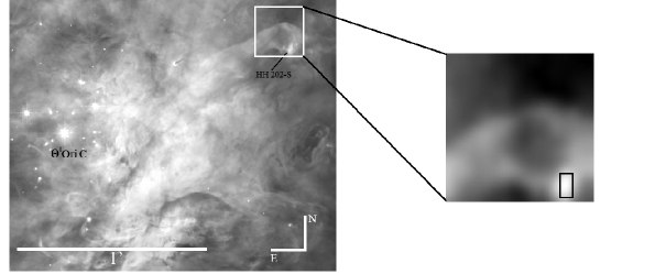
Figure 1: $HST$ image of the central part of the Orion Nebula combined with WFPC2 images in different filters (O’Dell & Wong, 1996). The white square corresponds to the field of view of the Potsdam Multi-Aperture Spectrograph (PMAS) and the separate close up image at the right shows the rebinned H$\alpha$ map presented in Paper I. Inside of this box, the black rectangle indicates the slit position and the area covered by the UVES spectrum analyzed in this paper (1$\aas@@fstack{\prime\prime}$5$\times$2$\aas@@fstack{\prime\prime}$5).

and the ADF for ${\rm O^{+}}$ and ${\rm O^{2+}}$. In §5 we discuss: a) some inconsistencies found in the Balmer decrement of the lines of higher principal quantum number, b) the ionization structure of HH 202-S, c) the radial velocity pattern of the lines of each kinematic component, d) the $t^{2}$ parameter obtained from different methods and its possible relation with the ADF, and e) the evidences of dust grain destruction in HH 202-S. Finally, in §6 we summarize our main conclusions.

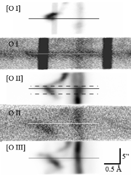
Figure 2: Sections of the bidimensional UVES spectrum showing the spatio-kinematic profiles of different oxygen lines: [O i] 6300 Å, O i 7772 Å, [O ii] 3728 Å, O ii 4649 Å and [O iii] 4959 Å. Wavelength increases to the right and north points up. The solid straight lines in all the sections correspond to the slit center and the dashed lines –only represented in the case of the [O ii] 3728 Å profile– correspond to the extracted area 2$\aas@@fstack{\prime\prime}$5 wide.

2 Observations and Data Reduction

HH 202 was observed on 2003 March 30 at Cerro Paranal Observatory (Chile), using the UT2 (Kueyen) of the Very Large Telescope (VLT) with the Ultraviolet Visual Echelle Spectrograph (UVES, D’Odorico et al., 2000). The standard settings of UVES were used covering the spectral range from 3100 to 10400 Å. Some narrow spectral ranges could not be observed. These are: 5783-5830 and 8540-8650 Å, due to the physical separation between the CCDs of the detector system of the red arm; and 10084-10088 and 10252-10259 Å, because the last two orders of the spectrum do not fit completely within the size of the CCD. Five individual exposures of 90 seconds –for the 3100-3900 and 4750-6800 Å ranges– and 270 seconds –for the 3800-5000 and 6700-10400 Å ranges– were added to obtain the final spectra. In addition, exposures of 5 and 10 seconds were taken to obtain good flux measurements –$i.e.$ non-saturated– for the brightest emission lines. The spectral resolution was $\lambda/\Delta\lambda\approx 30000$. This high spectral resolution enables us to separate two kinematic components: one corresponding to the ambient gas –which we will call nebular component and whose emission mainly arises from behind HH 202 and, therefore, could not entirely correspond to the pre-shock gas– and another one corresponding to the gas flow of the HH object, the post-shock gas, which we will call shock component.
The slit was oriented north-south and the atmospheric dispersion corrector (ADC) was used to keep the same observed region within the slit regardless of the air mass value. The HH object was observed between airmass values of 1.20 and 1.35. The average seeing during the observation was 0$\aas@@fstack{\prime\prime}$7. The slit width was set to 1$\aas@@fstack{\prime\prime}$5 as a compromise between the spectral resolution needed and the desired signal-to-noise ratio of the spectra. The slit length was fixed to 10$\arcsec$. The one-dimensional spectra were extracted for an area of 1$\aas@@fstack{\prime\prime}$5$\times$2$\aas@@fstack{\prime\prime}$5. This area covers the apex of HH 202, the so-called knot HH 202-S, as we can see in Figure 1. This zone shows the maximum shift in velocity between the shock and nebular components (see Figure 2) allowing us to appropriately separate and study the spectra of both kinematic components.
The spectra were reduced using the iraf echelle reduction package, following the standard procedure of bias subtraction, aperture extraction, flatfielding, wavelength calibration and flux calibration. The standard stars EG 247, C-32 9927 (Hamuy et al., 1992, 1994) and HD 49798 (Bohlin & Lindler, 1992; Turnshek et al., 1990) were observed to perform the flux calibration. The error of the absolute flux calibration was of the order of 3%.

3 Line measurements, identifications and reddening correction

Line fluxes were measured applying a double Gaussian profile fit procedure over the local continuum. All these measurements were made with the splot routine of iraf.
All line fluxes of a given spectrum have been normalized to a particular bright emission line present in the common range of two consecutive spectra. For the bluest spectrum (3100-3900 Å), the reference line was H9 3835 Å. For the range from 3800 to 5000 Å, the reference line was H$\beta$. In the case of the spectrum covering 4750-6800 Å, the reference was [O iii] 4959 Å. Finally, for the reddest spectrum (6700-10400 Å), the reference line was [S ii] 6731 Å. In order to produce a final homogeneous set of line flux ratios, all of them were rescaled to the H$\beta$ flux. In the case of the bluest spectra the ratios were rescaled by the H9/H$\beta$ ratio obtained from the 3800-5000 Å range. The emission line ratios of the 4750-6800 Å range were multipled by the [O iii] 4959/H$\beta$ ratio measured in the 3800-5000 Å range. In the case of the last spectral section, 6700-10400 Å, the rescaling factor was the [S ii] 6731/H$\beta$ ratio obtained from the 4750-6800 Å spectrum. All rescaling factors were measured in the short exposure spectra in order to avoid the possible saturation of the brightest emission lines. This process was done separately for both the nebular and shock components.
The spectral ranges present overlapping regions at the edges. The adopted flux of a line in the overlapping region was obtained as the average of the values obtained in both spectra. A similar procedure was considered in the case of lines present in two consecutive spectral orders of the same spectral range. The average of both measurements was considered for the adopted value of the line flux. In all cases, the differences in the line flux measured for the same line in different orders and/or spectral ranges do not show systematic trends and are always within the uncertainties.
The identification and laboratory wavelengths of the lines were obtained following a previous work on the Orion Nebula by Esteban et al. (2004), the compilations by Moore (1945) and The Atomic Line List v2.04. The

Figure 3: Section of the echelle spectrum of HH 202-S showing the shock (left) and nebular (right) components of each emission line of multiplet 1 of O ii.

identification process and the measurement of line fluxes were done simultaneously. The inspection of the line shapes at the bi-dimensional echelle spectrum was always used to identify which component –nebular or shock– was measured at each moment. The rather different spatial and spatio-kinematic structure of the two kinematic components is illustrated in Figure 2. We have identified 360 emission lines in the spectrum of HH 202-S, 115 of them only show one component –8 belong to the nebular component and 107 belong to the shock one– and 8 are dubious identifications.
For a given line, the observed wavelength is determined by the centroid of the Gaussian fit to the line profile. For lines measured in different orders and/or spectral ranges, the average of the different wavelength determinations has been adopted. From the adopted wavelength, the heliocentric velocity, $V_{hel}$, has been calculated using the heliocentric correction appropriate for the coordinates of the object and the moment of observation. The typical error in the heliocentric velocity measured is about 1-2 km s^-1.
All line fluxes with respect to H$\beta$, $F(\lambda)/F({\rm H}\beta)$, were dereddened using the typical relation,

$$\frac{I(\lambda)}{I({\rm H}\beta)}=\frac{F(\lambda)}{F({\rm H}\beta)}10^{c({\rm H}\beta)f(\lambda)}.$$ (1)

The reddening coefficient, c(H$\beta$), respresents the amount of interstellar extinction which is the logarithmic extinction at H$\beta$, while $f(\lambda)$ is the adopted extinction curve normalized to $f({\rm H}\beta)=0$. The reddening coefficient was determined from the comparison of the observed flux ratio of Balmer and Paschen lines –those not contaminated by telluric or other nebular emissions– with respect to H$\beta$ and the theoretical ones computed by Storey & Hummer (1995) for the physical conditions of $T_{e}$ $=$ 10000 K and $n_{e}$ $=$ 1000 cm^-3. As in Paper I, we have used the reddening function, $f(\lambda)$, normalized to H$\beta$ derived by Blagrave et al. (2007) for the Orion Nebula. The use of this extinction law instead of the classical one (Costero & Peimbert, 1970) produces slightly higher c(H$\beta$) values and also slightly different dereddened line fluxes depending on the spectral range (see Paper I). The final c(H$\beta$) values obtained for the two kinematic components were weighted averages of the values obtained for the individual lines: c(H$\beta$)_neb $=$ 0.41$\pm$0.02 and c(H$\beta$)_sh $=$ 0.45$\pm$0.02. Although not all the c(H$\beta$) values are consistent with each other (see §5.1), the average values obtained are quite similar and consistent within the uncertainties.
We can compare the reddening values with those obtained from integral field spectroscopy data presented in Paper I in the same area of HH 202-S (see Figure 1) and corresponding to the section $\Delta\alpha$ $=$ $[-4,-6]$ and $\Delta\delta$ $=$ $[-8,-5]$ (see Figure 3 of Paper I). The average c(H$\beta$) in this zone is 0.65$\pm$0.15, which is higher than those determined for UVES data. However, if we re-calculate the value of c(H$\beta$) from the UVES data using the same Balmer lines as in Paper I, we obtain a value 0.5$\pm$0.1 in both kinematic components, a value consistent with the PMAS one within the errors. These differences can be related to several systematical disagreements found between the c(H$\beta$) values obtained from different individual Balmer or Paschen lines (see §5.1).
In the most complete work on the reddening distribution across the Orion Nebula, O’Dell & Yusef-Zadeh (2000) obtain values of c(H$\beta$) between 0.2 and 0.4 in the zone around HH 202-S, somewhat lower than our reddening determinations. This can be due to the fact that O’Dell & Yusef-Zadeh use the extinction law by Costero & Peimbert (1970) which, as we discuss in Paper I, produces lower c(H$\beta$) values than the more recent extinction law (Blagrave et al., 2007). We have also re-calculated c(H$\beta$) from our UVES spectra making use of the Costero & Peimbert law, and we obtain values about 0.3, being now in agreement with the determinations of O’Dell & Yusef-Zadeh (2000).
In Table 3, the final list of line identifications (columns 1–3), $f(\lambda)$ values (column 4), heliocentric velocities (columns 5 and 8) and dereddened flux line ratios (columns 6 and 9) for the nebular and shock component are presented. The observational errors associated with the line dereddened fluxes with respect to H$\beta$ –in percentage– are also presented in columns (7) and (10) of Table 3. These errors include the uncertainties in line flux measurement, flux calibration and error propagation in the reddening coefficient.
In column (11) of Table 3, we present the shock-to-nebular line flux ratio for those lines in which both kinematic components have been measured. This ratio is defined as:

$$\frac{I_{\rm sh}}{I_{\rm neb}}=\frac{[I(\lambda)/I({\rm H}\beta)]_{\rm sh}}{[I(\lambda)/I({\rm H}\beta)]_{\rm neb}}=\frac{I(\lambda)_{\rm sh}}{I(\lambda)_{\rm neb}}\times\frac{I({\rm H}\beta)_{\rm neb}}{I({\rm H}\beta)_{\rm sh}}$$ (2)

where the integrated dereddened H$\beta$ fluxes are $I$(H$\beta$)_neb $=$ (3.80$\pm$0.20)$\times$10^-12 erg cm^-2 s^-1 and $I$(H$\beta$)_sh $=$ (6.00$\pm$0.20)$\times$10^-12 erg cm^-2 s^-1. The $I$_neb/$I$_sh ratios depend on each particular line. In general, they are close to 1 for H i lines but become less than 1 for higher ionized species –except Fe ions–, and are typically greater than 1 for neutral species. A more extensive discussion on this particular issue will be presented in section §5.2.
In Figure 3, we show a section of our flux-calibrated echelle spectra around the lines of multiplet 1 of O ii. It can be seen that both the nebular and the shock components are well separated and show a remarkable high signal-to-noise ratio.

Table 1: Identifications, reddening-corrected line ratios (I(H$\beta$)=100) for an area of 1$\aas@@fstack{\prime\prime}$5$\times$2$\aas@@fstack{\prime\prime}$5 and heliocentric velocities for the nebular and shock components.

				Nebular Component			Shock Component
$\lambda_{0}$ (Å)a	Iona	Multa	$f(\lambda)^{b}$	$V_{hel}$c	$I$($\lambda$)d	Error (%)e	$V_{hel}$c	$I$($\lambda$)d	Error (%)e	$I$sh/$I$nebf	Notes
3187.74	He i	3	0.195	15	3.450	6	-34	3.682	6	1.067
3239.74	[Fe iii]	6F	0.194	-	-	-	-35	0.806	15	-
3286.19	[Fe iii]	6F	0.192	-	-	-	-35	0.206	15	-
3319.21	[Fe iii]	6F	0.191	-	-	-	-38	0.114	40	-
3322.54	[Fe iii]	5F	0.191	-	-	-	-48	0.744	9	-
3334.90	[Fe iii]	6F	0.190	-	-	-	-36	0.320	9	-
3354.55	He i	8	0.189	14	0.148	10	-33	0.159	10	1.079
3355.49	[Fe iii]	6F	0.189	-	-	-	-37	0.189	10	-
3356.57	[Fe iii]	6F	0.189	-	-	-	-35	0.262	9	-
3366.20	[Fe iii]	6F	0.189	-	-	-	-35	0.119	40	-
3371.41	[Fe iii]	5F	0.188	-	-	-	-47	0.543	11	-
3406.18	[Fe iii]	5F	0.186	-	-	-	-48	0.250	11	-
3447.59	He i	7	0.184	16	0.241	9	-34	0.246	9	1.019
3498.66	He i	40	0.180	10	0.090	15	-36	0.054	18	0.595
3512.52	He i	38	0.179	13	0.195	10	-38	0.176	10	0.901
3530.50	He i	36	0.178	12	0.129	10	-34	0.147	10	1.136
3554.42	He i	34	0.176	15	0.224	10	-36	0.219	10	0.976
3587.28	He i	32	0.173	13	0.331	9	-36	0.339	9	1.024
3613.64	He i	6	0.171	15	0.435	9	-37	0.462	9	1.061
3634.25	He i	28	0.169	13	0.425	9	-35	0.464	9	1.090
3664.68	H i	H28	0.166	13	0.172	10	-36	0.251	9	1.457
3666.10	H i	H27	0.166	13	0.355	9	-36	0.347	9	0.977
3667.68	H i	H26	0.166	13	0.414	9	-36	0.458	9	1.105
3669.47	H i	H25	0.166	13	0.468	9	-36	0.502	9	1.072
3671.48	H i	H24	0.165	13	0.543	9	-36	0.586	9	1.079
3673.76	H i	H23	0.165	14	0.557	9	-36	0.645	9	1.157
3676.37	H i	H22	0.165	15	0.661	9	-36	0.721	9	1.091
3679.36	H i	H21	0.165	15	0.761	9	-36	0.841	9	1.105
3682.81	H i	H20	0.164	14	0.822	9	-36	0.887	9	1.079
3686.83	H i	H19	0.164	15	0.867	9	-36	0.993	9	1.146
3691.56	H i	H18	0.163	14	1.106	9	-37	1.148	9	1.038
3697.15	H i	H17	0.163	14	1.271	6	-36	1.312	6	1.032
3703.86	H i	H16	0.162	13	1.409	6	-37	1.502	6	1.065
3705.04	He i	25	0.162	10	0.646	9	-39	0.717	9	1.108
3711.97	H i	H15	0.161	14	1.745	6	-36	1.834	6	1.050
3721.83	[S iii]	2F	0.160	10	4.041	6	-39	3.363	6	0.832
3721.93	H i	H14
3726.03	[O ii]	1F	0.160	22	87.30	5	-34	70.12	5	0.803
3728.82	[O ii]	1F	0.160	18	52.04	5	-36	28.15	5	0.540
3734.37	H i	H13	0.159	13	2.542	6	-36	2.581	6	1.015
3750.15	H i	H12	0.158	14	3.081	6	-36	3.143	6	1.020
3770.63	H i	H11	0.155	14	3.967	6	-36	4.087	6	1.030
3797.63	[S iii]	2F	0.152	35	5.240	5	-15	5.381	5	1.027
3797.90	H i	H10
3805.74	He i	58	0.152	12	0.063	15	-37	0.045	18	0.720
3819.61	He i	22	0.150	14	1.129	9	-35	1.153	7	1.020
3833.57	He i	62	0.149	14	0.067	15	-39	0.077	15	1.158
3835.39	H i	H9	0.148	13	7.271	6	-37	7.242	6	0.996
3856.02	Si ii	1	0.146	16	0.211	10	-38	0.309	10	1.469
3862.59	Si ii	1	0.145	16	0.120	12	-38	0.175	12	1.450
3868.75	[Ne iii]	1F	0.145	12	12.94	5	-34	8.096	6	0.625
3871.82	He i	60	0.144	10	0.084	15	-39	0.087	15	1.034
3888.65	He i	2	0.142	16	6.717	6	-39	5.625	6	0.837
3889.05	H i	H8	0.142	13	11.52	4	-45	9.043	6	0.784
3918.98	C ii	4	0.139	9	0.049	18	-39	0.062	18	1.267
3920.68	C ii	4	0.139	9	0.098	15	-39	0.106	15	1.086
3926.53	He i	58	0.138	15	0.122	10	-36	0.135	10	1.102
3964.73	He i	5	0.133	13	0.906	9	-36	0.937	9	1.034
3967.46	[Ne iii]	1F	0.133	13	3.866	6	-36	2.574	6	0.665
3970.07	H i	H7	0.133	13	15.68	4	-37	15.93	4	1.016
3993.06	[Ni ii]	4F	0.130	28	0.033	20	-40	0.041	18	1.227
4008.36	[Fe iii]	4F	0.128	-	-	-	-42	0.587	9	-	$g$

^a

Identification of each line: laboratory wavelength, ion and multiplet.

^b

Value of the extinction curve adopted (Blagrave et al., 2007).

^c

Heliocentric velocity in units of km s^-1, the typical error is 1-2 km s^-1.

^d

Dereddened fluxes with respect to $I$(H$\beta$) = 100.

^e

Error of the dereddened flux ratios. Colons indicate errors larger than 40 per cent.

^f

Shock-to-nebular line flux ratio. See definition in equation (2).

^g

Line blended with another line and deblended via Gaussian fitting.

^h

Contaminated by “ghost”.

ⁱ

Contaminated by telluric emissions and not deblended.

^j

Deblended from telluric emissions.

4 Results

4.1 Excitation mechanism of the ionized gas in HH 202-S

In their recent work, O’Dell & Henney (2008) argue that the presence of a variety of ionization stages in the ionized gas of HH 202 indicates that the flow also contains neutral material. They interpret that fact as due to the impact of the flow with preexisting neutral material –perhaps of the foreground veil– or that the flow compresses the ambient ionized gas inside the nebula to such degree that it traps the ionization front. Our results provide some clues that can help to ascertain this issue. The value of some emission line ratios are good indicators of the presence of shock excitation in ionized gas, especially [S ii]/H$\alpha$ and [O i]/H$\alpha$. In our spectra, we find log([S ii] 6717+31/H$\alpha$) values which are almost identical in both kinematic components ($-$1.49 and $-$1.44 for the nebular and shock component, respectively). These values are completely consistent with those expected for photoionized nebulae and far from the range of values between $-$0.5 and 0.5, which is the typical of supernova remnants and HH objects (see Figure 10 of Riera et al., 1989). On the other hand, the values of log([O i] 6300/H$\alpha$) that we obtain for the nebular and shock component are of $-$2.66 and $-$2.22, somewhat different in this case, but also far from the values expected in the case of substantial contribution of shock excitation (Hartigan et al., 1987). Finally, we have also used the diagnostic diagrams of Raga et al. (2008) where the [N ii] 6548/H$\alpha$ and [S ii] 6717+31/H$\alpha$ $vs.$ [O iii] 5007/H$\alpha$ ratios of HH 202 are found in the zone dominated by photoionized shocks. Therefore, the spectrum of HH 202-S seems to be consistent with the picture that the bulk of the emission in this area is produced by photoionization acting on compressed ambient gas that has trapped the ionization front inside the ionized bubble of the nebula. In the rest of the paper we will provide and discuss further indications that HH 202-S contains an ionization front.

4.2 Physical Conditions

We have computed physical conditions of the two kinematic components using several ratios of CELs following the same methodology as in Paper I and in Mesa-Delgado et al. (2008a). The electron temperatures, $T_{e}$, and densities, $n_{e}$, are presented in Table LABEL:cond. We have determined $n_{e}$ from [O ii], [S ii], [Cl iii] and [Ar iv] line ratios using the nebular package (Shaw & Dufour, 1995). In the case of the $n_{e}$ obtained from [Fe iii] lines, we have used flux ratios of 31 and 12 lines for the shock and nebular component, respectively, following the procedure described by García-Rojas et al. (2006). For the nebular component, we have adopted the average value of $n_{e}$([O ii]), $n_{e}$([S ii]) and $n_{e}$([Cl iii]) excluding $n_{e}$([Fe iii]) and $n_{e}$([Ar iv]) due to their discrepant values and very large uncertainties. For the shock component, we have adopted the average of $n_{e}$([O ii]), $n_{e}$([Cl iii]) and $n_{e}$([Fe iii]), while $n_{e}$([S ii]) has not been included because the [S ii] line ratio is out of the range of validity of the indicator. As we can see in Table LABEL:cond, the density of the shock component ($\sim$17000 cm^-3) is much higher than the density of the nebular one ($\sim$3000 cm^-3). However, the bulk of the emission of the nebular component might come from behind HH 202, and the electron density that we have found for that component might not be the true one of the pre-shock gas. In fact, taking into account that the velocity of the gas flow is 89 km s^-1 (O’Dell & Henney, 2008) and the typical sound speed of an ionized gas is about 10-20 km s^-1, we have adopted a Mach number, $M$, for HH 202 of about 5 and, thus, the shock compression ratio should be $M^{2}\sim 25$. Using the density of the shock component (see Table LABEL:cond), we obtain a pre-shock density $\sim 17430/25\approx 700$ cm^-3. This value is lower than the 2890 cm^-3 determined for the nebular component. Therefore, it seems clear that the bulk of the nebular component does not refer to the gas in the immediate vicinity of HH 202 as we have mentioned in §2. Electron temperatures have been derived from the classical CEL ratios of [N ii], [O ii], [S ii], [O iii], [S iii] and [Ar iii]. Under the two-zone ionization scheme we have adopted $T_{e}$([N ii]) as representative for the low ionization zone and $T_{e}$([O iii]) for the high ionization zone. We have also derived $T_{e}$(He i) using the method of Peimbert et al. (2002) and state-of-the-art atomic data (see §4.4). We have compared these temperature determinations with those obtained from the integral field unit (IFU) data presented in Paper I. We have determined the mean $T_{e}$ values of the spaxels of the section of the FOV of the PMAS data that encompasses the area covered by our UVES spectrum, finding $<$$T_{e}$([O iii])$>$ = 8760$\pm$260 K and $<$$T_{e}$([N ii])$>$ = 9730$\pm$590 K. These values are in agreement within the errors with those obtained in this paper (see Table LABEL:cond). The average density from the IFU data, obtained from the [S ii] line ratio, is 7300$\pm$3000 cm^-3, a value between the $n_{e}$ adopted for each kinematic component from the UVES data. As we can see in Table LABEL:cond, the $T_{e}$ values are quite similar in both components with differences of the order of a few 100 K. The temperatures derived from [N ii] lines are higher than those derived from [O iii] lines, which is a typical result observed in previous works on the Orion Nebula (e.g. Mesa-Delgado et al., 2008a; Rubin et al., 2003), as well as in Paper I. This is a likely result of the ionization stratification in the nebula. It is interesting to note that the difference between both temperatures is smaller in the case of the shock component, in this case, all the emission comes from a –probably– much narrower slab of ionized gas. The relatively low uncertainties in the physical conditions are due to the high signal-to-noise ratio of the emission lines used in the diagnostics. Blagrave et al. (2006) computed the physical conditions for HH 529 and they obtained similar results –higher densities in the shock component but similar temperatures in both components– though with comparatively larger errors.

4.3 Ionic abundances from CELs

Ionic abundances of ${\rm N^{+}}$, ${\rm O^{+}}$, ${\rm O^{2+}}$, ${\rm Ne^{2+}}$, ${\rm S^{+}}$, ${\rm S^{2+}}$, ${\rm Cl^{+}}$, ${\rm Cl^{2+}}$, ${\rm Ar^{2+}}$ and ${\rm Ar^{3+}}$ have been derived from CELs under the two-zone scheme and $t^{2}$$=$ 0, using the nebular package. All abundances were calculated for the shock and nebular component, except for ${\rm Ar^{3+}}$, which was not detected in the spectrum of the shock component. The atomic data for ${\rm Cl^{+}}$ are not implemented in the nebular routines, so we have used an old version of the 5-level atom program of Shaw & Dufour (1995) –fivel– that is described by De Robertis et al. (1987). This program uses the atomic data for this ion compiled by Mendoza (1983). We have also measured [Ca ii], [Cr ii], [Fe ii], [Fe iii], [Fe iv], [Ni ii] and [Ni iii] lines. The abundances of these ions are also presented in Table LABEL:abioni. They were computed assuming the appropriate temperature under the two-zone scheme and the procedures indicated below. In addition and only in the shock component, we have detected a substantial number of lines of other quite rare heavy-element ions as [Cr iii], [Co ii], [Co iii], [Ti iii] and, possibly, [Cr iv], [Co iv], [Mn ii] and [V ii]. Unfortunately, we cannot derive abundances from these lines due to the lack of atomic data for these ions. Two [Ca ii] lines at 7291 and 7324 Å were detected in the shock component. In order to derive the ${\rm Ca^{+}}$ abundance, we solved a 5-level model atom using the single atomic dataset available for this ion (Meléndez et al., 2007). Note that this is the first determination of the ${\rm Ca^{+}}$ abundance in the Orion Nebula and this poses a lower limit to the gas-phase Ca/H ratio in this object. Two and four [Cr ii] lines were measured in the nebular and shock component, respectively, although those at 8309 and 8368 Å are very faint. [Cr ii] lines can be affected by continuum or starlight fluorescence as is also the case for the [Fe ii] and [Ni ii] lines. We have computed the ${\rm Cr^{+}}$ abundances using a 180-level model atom that treat continuum fluorescence excitation as in Bautista et al. (1996) and includes the atomic data of Bautista et al. (2008). In order to consider the continuum fluorescence excitation we have assumed that the incident radiation field derives entirely from the dominant ionization star $\theta^{1}$ Ori C. As Bautista et al. (1996), we have calculated a dilution factor assuming a $T_{eff}$ = 39000 K, $R_{star}$ = 9.0$R_{\odot}$ (see §5.3) and a distance to the Orion Nebula of 414 pc (Menten et al., 2007). In Table LABEL:abioni, we include the ${\rm Cr^{+}}$/${\rm H^{+}}$ ratio for the nebular and shock component. This is the first estimation of the ${\rm Cr^{+}}$ abundance in the Orion Nebula. Several [Fe ii] lines have been detected in our spectra. As in the case of [Cr ii] lines, most of them are affected by continuum fluorescence (see Rodríguez, 1999; Verner et al., 2000). Following the same procedure as for ${\rm Cr^{+}}$, we considered a 159 model atom in order to compute the ${\rm Fe^{+}}$ abundances using the atomic data presented in Bautista & Pradhan (1998). Many [Fe iii] lines have been detected in the two kinematic components and their flux is not affected by fluorescence. For the calculations of the ${\rm Fe^{2+}}$/${\rm H^{+}}$ ratio, we have implemented a 34-level model atom that uses collision strengths taken from Zhang (1996) and the transition probabilities of Quinet (1996) as well as the new transitions found by Johansson et al. (2000). The average value of the ${\rm Fe^{2+}}$ abundance has been obtained from 31 and 12 individual emission lines for the shock and nebular component, respectively. One [Fe iv] line has been detected in the shock component at 6740 Å. The ${\rm Fe^{3+}}$/

^a

In units of 12+log(${\rm X^{+n}}$/${\rm H^{+}}$) .

^b

Average value from positions 8b and 11 of Walter et al. (1992).

${\rm H^{+}}$ ratio has been derived using a 33-level model atom where all collision strengths are those calculated by Zhang & Pradhan (1997) and the transition probabilities recommended by Froese Fischer & Rubin (2004). Several [Ni ii] lines have been measured in both kinematic components but they are strongly affected by continuum fluorescence (see Lucy, 1995). As for the ${\rm Cr^{+}}$ and ${\rm Fe^{+}}$ ions, we have used a 76-level model that includes continuum fluorescence excitation and the new collisional data of Bautista (2004) in order to compute the ${\rm Ni^{+}}$ abundances. We have measured several [Ni iii] lines in the shock and nebular components. These lines are not expected to be affected by fluorescence. The ${\rm Ni^{2+}}$/${\rm H^{+}}$ ratio has been derived using a 126-level model atom and the atomic data of Bautista (2001). The final adopted values of the ionic abundances are listed in columns (1) and (3) of Table LABEL:abioni for the nebular and shock component, respectively. Columns (2) and (4) correspond to the ionic abundances of both components assuming the presence of temperature fluctuations (see §5.5). In this table, we have also included the ${\rm C^{2+}}$/${\rm H^{+}}$ ratio obtained from UV CELs by Walter et al. (1992). We have taken the average of the values corresponding to their slit positions 8b and 11, the nearest positions to HH 202. The uncertainties shown in the table are the quadratic sum of the independent contributions of the error in the density, temperature and line fluxes. The abundance determinations presented in Table LABEL:abioni show the following behaviour: ionic abundances determined from CELs of once ionized species are always higher in the shock than in the nebular component; the twice ionized species of elements lighter than Ne (included), show lower abundances in the shock than in the nebular component; and the twice ionized species of elements heavier than Ne show similar abundances in both components except for iron, chromium and nickel abundances that show substantially larger abundances in the shock component, something that can be explained if a significant dust destruction occurs in this component (see §5.6). Finally, we have compared our abundance determinations from UVES data with those obtained in the HH 202-S region from the IFU data presented in Paper I. Integrating the spaxels of the section of the FOV indicated in §3, we obtain 12+log(${\rm O^{2+}}$/${\rm H^{+}}$) = 8.18$\pm$0.07 from CELs, which is in good agreement with the numbers presented in Table LABEL:abioni for both kinematic components. On the other hand, the average value of the ${\rm O^{+}}$ abundance from CELs is 8.06$\pm$0.l4. However, considering the large density dependence of this ionic abundance, we have recalculated the ${\rm O^{+}}$/${\rm H^{+}}$ ratio adopting the physical conditions measured in the shock component from UVES, finding a value of 8.26$\pm$0.09, which is in better agreement with the UVES determinations for the shock component, the brightest one in the [O ii] line emission.

4.4 Ionic abundances from RLs

We have measured several He i emission lines in the spectra of HH 202, both in the nebular and in the shock components. These lines arise mainly from recombination, but they can be affected by collisional excitation and self-absorption effects. We have used the effective recombination coefficients of Storey & Hummer (1995) for H i and those computed by Porter et al. (2005), with the interpolation formulae provided by Porter et al. (2007) for He i. The collisional contribution was estimated from Sawey & Berrington (1993) and Kingdon & Ferland (1995), and the optical depth in the triplet lines was derived from the computations by Benjamin et al. (2002). We have determined the He⁺/H⁺ ratio from a maximum likelihood method (MLM, Peimbert et al., 2000; Peimbert et al., 2002). To self-consistently determine $n_{e}$(He i), $T_{e}$(He i), ${\rm He^{+}}$/${\rm H^{+}}$ and the optical depth in the He i 3889 line, $\tau_{3889}$, we have used the adopted density obtained from the CEL ratios for each component as $n_{e}$(He i) (see Table LABEL:cond) and a set of 16 He i lines (at 3614, 3819, 3889, 3965, 4026, 4121, 4388, 4471, 4713, 4922, 5016, 5048, 5876, 6678, 7065 and 7281 Å). We have discarded the He i 5048 Å line in the nebular component because it is affected by charge transfer in the CCD. So, for the nebular component of HH 202, we have a total of 16 observational constraints (15 lines plus $n_{e}$), and for the shock component, we have 17 observational constraints (16 lines plus $n_{e}$). Finally, we have obtained the best value for the 3 unknowns and $t^{2}$ by minimizing $\chi^{2}$. The final $\chi^{2}$ parameters we have obtained are 7.53 for the nebular component and 12.34 for the shock component, which indicate very good fits, taking into account the degrees of freedom. The final adopted value of the ${\rm He^{+}}$/${\rm H^{+}}$ ratio for each component is included in Table LABEL:abioni. We have detected C ii lines of multiplets 2, 3, 4, 6 and 17.02. The brightest of these lines is C ii 4267 Å, which belongs to multiplet 6 and can be used to derive a proper ${\rm C^{2+}}$/${\rm H^{+}}$ ratio. The rest of the C ii lines are affected by fluorescence, like multiplets 2, 3 and 4 (see Grandi, 1976) or are very weak, as in the case of the line multiplet 17.02 that has an uncertainty of 40% in the line flux. We have derived the ${\rm O^{+}}$/${\rm H^{+}}$ ratio from RLs for the shock and nebular components. The O i lines of multiplet 1 are very weak and they are partially blended with bright telluric emission. In order to obtain the best possible abundance determination, we have used different lines for each component: O i 7775 Å for the nebular component and O i 7772 Å for the shock one, these are precisely the lines least affected by line-blending. The high signal-to-noise of the spectra allowed us to detect and measure seven lines of the multiplet 1 of O ii as we can see in Figure 3. These lines are affected by non-local thermal equilibrium (NLTE) effects (Ruiz et al., 2003), therefore to obtain a correct ${\rm O^{2+}}$ abundance it is necessary to observe the eight lines of the multiplet. However, these effects are rather small in the Orion Nebula –as well as in the observed components– due to its relatively large density. Then, assuming LTE, the ${\rm O^{2+}}$ abundance from RLs has been calculated considering the abundances obtained from the flux of each line of multiplet 1 and the abundance from the estimated total flux of the multiplet (see Esteban et al., 1998). The abundance determinations in Table LABEL:abioni show that the ${\rm He^{+}}$/${\rm H^{+}}$, ${\rm C^{2+}}$/${\rm H^{+}}$ and ${\rm O^{2+}}$/${\rm H^{+}}$ ratios derived from RLs are always very similar in both shock and nebular component. In the case of ${\rm O^{+}}$ abundances, the nominal values determined for both components seem to be somewhat different (about 0.24 dex), but they are marginally in agreement considering the large uncertainties of this ion abundance. As in the previous subsection, we have compared our abundance determinations from RLs with those obtained for HH 202-S in Paper I. From the data of Paper I, we obtain 12$+$log(${\rm O^{2+}}$/${\rm H^{+}}$) $=$ 8.39$\pm$0.13 and 12$+$log(${\rm C^{2+}}$/${\rm H^{+}}$) $=$ 8.29$\pm$0.11, values which are in good agreement with those obtained in this paper.

4.5 Abundance discrepancy factors

We have calculated ionic abundances from two kinds of lines –RLs and CELs– for three ions: ${\rm C^{2+}}$, ${\rm O^{+}}$ and ${\rm O^{2+}}$. We present their values for the two components in Table LABEL:abioni. We have computed the ADF for these ions using the following definition:

$${\rm ADF(X^{+i})=log\Big{(}\frac{X^{+i}}{H^{+}}\Big{)}_{RL}-log\Big{(}\frac{X^{+i}}{H^{+}}\Big{)}_{CEL}.}$$ (3)

In the case of the ADF(${\rm C^{2+}}$) it can only be estimated for the nebular component and from the comparison of our determination from RLs and those from CELs for nearby zones taken from the literature. The value of the ADF(${\rm C^{2+}}$) amounts to 0.45 dex. On the one hand, the ADF(${\rm O^{+}}$) can also be estimated in our spectrum and shows values very close to zero. However, these ADF values are rather uncertain. On the other hand, as we can see in Table LABEL:abioni, the ${\rm O^{2+}}$ abundance from RLs is the same for both components while that from CELs is lower in the shock component, probably because the recombination rate increases in the shock one. This fact produces an ${\rm ADF(O^{2+})}$ about 0.2 dex higher in the shock component than in the nebular one. This striking result will be discussed in section §5.5. The values of the ADFs of ${\rm C^{2+}}$ and ${\rm O^{2+}}$ for the nebular component are in good agreement with those obtained by Esteban et al. (2004) for a zone closer to the Trapezium cluster than HH 202. In the case of the ADF(${\rm O^{+}}$), both determinations disagree, Esteban et al. (2004) report a much larger value (0.39 dex).

4.6 Total abundances

^a

From photoionization models by Garnett et al. (1999).

^b

Mean of Orion Nebula models.

^c

From correlations obtained by Martín-Hernández et al. (2002).

^d

From photoionization models by Rodríguez & Rubin (2005).

In order to derive the total gaseous abundances of the different elements present in our spectrum, we have to correct for the unseen ionization stages by using a set of ionization correction factors (ICFs). The adopted ICF values are presented in Table LABEL:icf and the total abundances in Table LABEL:abtot. As in the case of the ionic abundances from CELs, these tables include values under the assumption of $t^{2}$$=$ 0 –columns (1) and (3)– and under the presence of temperature fluctuations (see §5.5) –columns (2) and (4)–. The total helium abundance has been corrected for the presence of neutral helium using the expression proposed by Peimbert et al. (1992) based on the similarity of the ionization potentials of ${\rm He^{0}}$ (24.6 eV) and ${\rm S^{+}}$ (23.3 eV).

$${\rm\frac{He}{H}=\big{(}1+\frac{S^{+}}{S-S^{+}}\big{)}\times\frac{He^{+}}{H^{+}}=ICF(He^{0})\times\frac{He^{+}}{H^{+}}},$$ (4)

For C we have adopted the ICF(${\rm C^{+}}$) derived from photoionization models of Garnett et al. (1999) for the shock and nebular component. In order to derive the total abundance of nitrogen we have used the usual ICF:

$${\rm\frac{N}{H}=\frac{O^{+}+O^{2+}}{O^{+}}\times\frac{N^{+}}{H^{+}}=ICF(N^{2+})\times\frac{N^{+}}{H^{+}}}.$$ (5)

This expression gives very different values of the ICF(${\rm N^{2+}}$) for both components due to their rather different ionization degree. The total abundance of oxygen is calculated as the sum of ${\rm O^{+}}$ and ${\rm O^{2+}}$ abundances. The absence of He ii lines in the spectra and the similarity between the ionization potentials of ${\rm He^{+}}$ and ${\rm O^{2+}}$, implies the absence of ${\rm O^{3+}}$. In Table LABEL:abtot we present the O abundances from RLs and CELs. The only measurable CELs of Ne in the optical range are those of ${\rm Ne^{2+}}$ but the fraction of ${\rm Ne^{+}}$ can be important in the nebula. We have adopted the usual expression (Peimbert & Costero, 1969) to obtain the total Ne abundance:

$${\rm\frac{Ne}{H}=\frac{O^{+}+O^{2+}}{O^{2+}}\times\frac{Ne^{2+}}{H^{+}}=ICF(Ne^{+})\times\frac{Ne^{2+}}{H^{+}}}.$$ (6)

We have measured CELs of two ionization stages of S: ${\rm S^{+}}$ and ${\rm S^{2+}}$. Then, we have used an ICF to take into account the presence of ${\rm S^{3+}}$ (Stasińska, 1978) which is based on photoionization models of H ii regions.

$${\rm\frac{S}{H}=\Big{(}1-\big{[}\frac{O^{+}}{O^{+}+O^{2+}}\big{]}^{3}\Big{)}^{-1/3}\times\frac{S^{+}+S^{2+}}{H^{+}}=}$$

$${\rm=ICF(S^{3+})\times\frac{S^{+}+S^{2+}}{H^{+}}}.$$ (7)

Following Esteban et al. (1998), we expect that the amount of ${\rm Cl^{3+}}$ is negligible in the Orion Nebula. Therefore, the total abundance of chlorine is simply the sum of ${\rm Cl^{+}}$ and ${\rm Cl^{2+}}$ abundances. For argon, we have determinations of ${\rm Ar^{2+}}$ and ${\rm Ar^{3+}}$ but some contribution of ${\rm Ar^{+}}$ is expected. In Table LABEL:icf we present the values obtained from two ICF schemes: one obtained from correlations between ${\rm N^{2+}}$/${\rm N^{+}}$ $vs.$ ${\rm Ar^{2+}}$/${\rm Ar^{+}}$ from ISO observations of compact H ii regions by Martín-Hernández et al. (2002) and another one –following Osterbrock et al. (1992)– derived as the mean of Orion Nebula models by Rubin et al. (1991) and Baldwin et al. (1991). We have measured lines of three ionization stages of iron in the shock component –${\rm Fe^{+}}$, ${\rm Fe^{2+}}$ and ${\rm Fe^{3+}}$– and two stages of ionization in the nebular component –${\rm Fe^{+}}$ and ${\rm Fe^{2+}}$–. For the shock component, we can derive the total Fe abundance from the sum of the three ionization stages. For the nebular component –and also for the shock one in order to compare– we have used an ICF scheme based on photoionization models of Rodríguez & Rubin (2005) to obtain the total Fe/H ratio using only the ${\rm Fe^{2+}}$ abundances, which is given by:

$${\rm\frac{Fe}{H}=0.9\times\Big{(}\frac{O^{+}}{O^{2+}}\Big{)}^{0.08}\times\frac{Fe^{2+}}{O^{+}}\times\frac{O}{H}}.$$ (8)

Finally, there is no ICF available in the literature to correct for the presence of ${\rm Ni^{3+}}$ in order to calculate the total Ni abundance. Nevertheless, we have applied a first order ICF scheme based on the similarity between the ionization potentials of ${\rm Ni^{3+}}$ (35.17 eV) and ${\rm O^{2+}}$ (35.12 eV):

$${\rm\frac{Ni^{3+}}{Ni}=\frac{O^{2+}}{O}}.$$ (9)

Therefore,

$${\rm\frac{Ni}{H}=\frac{O}{O^{+}}\times\Big{(}\frac{Ni^{+}}{H^{+}}+\frac{Ni^{2+}}{H^{+}}\Big{)}}.$$ (10)

In general, the total abundances shown in columns (1) and (3) of Table LABEL:abtot are quite similar for the shock and nebular component within the errors, except for the nickel and iron abundances, which are much larger in the shock component –see section §5.6 for a possible explanation. The set of abundances for the nebular component are in very good agreement with previous results of Esteban et al. (2004). We have also compared our Ni abundance values with the previous determination of Osterbrock et al. (1992) finding that our Ni/H ratio for the nebular component is an order of magnitud lower. This difference is due to the large uncertainties in the atomic data used by those authors (see Bautista, 2001).

^a

In units of 12+log(${\rm X^{+n}}$/${\rm H^{+}}$) .

^b

Average value from positions 8b and 11 of Walter et al. (1992).

^c

Value derived from RLs.

^d

Adopting the ICF from the mean of Orion Nebula models.

^e

Adopting the ICF from ISO observations (Martín-Hernández et al., 2002).

^f

From ${\rm Fe^{+}}$$+$${\rm Fe^{2+}}$$+$${\rm Fe^{3+}}$.

^g

Assuming the ICF of equation (6).

5 Discussion

5.1 Differences between the c(H$\beta$) coefficient determined with different lines

A puzzling feature of our UVES data is that the c$(\rm{H}\beta)$ values determined with different lines ratios appear to be inconsistent with each other, even with observational errors taken into account. Possible explanations are either a bias in the extinction curve or an extra mechanism, in addition to extinction, altering the individual line intensities from case B predictions. Figure 4 shows the c$(\rm{H}\beta)$ values measured for individual line ratios in the Balmer and Paschen series. The bizarre pattern followed by the curve, and particularly the steep slope it reaches in the proximity of the Balmer and Paschen limits, strongly suggest that the solution cannot be a bias in the extinction law. We can test the second hypothesis by considering how the line intensity ratios relative to case B ratios depend on the principal quantum number $n$ of the level where each line originates. Such dependence, plotted in Figure 5 for the two kinematic components, shows a definite trend with $n$ for both series. This strongly supports the second of our hypotheses, namely that an extra mechanism is acting to deviate level populations away from case B predictions. Indeed, detailed photoionization modeling indicates that this behaviour is the result of two independent but concomitant mechanisms: $\ell$-changing collisions with $|\Delta\ell|>1$ and pumping of Balmer and Paschen lines by absorption of stellar continuum photons at the Lyman wavelengths. Both mechanisms are neglected in case B calculations (Storey & Hummer, 1995) but included in our models, which take advantage of a new model hydrogen atom with fully resolved levels (Cloudy, version C08.00; Porter, Ferland, van Hoof, & Williams, in preparation; see also Appendix A in Luridiana et al. 2009); both alter the $n,\ell$ populations, resulting in enhanced intensities of the high $n$ lines. As for the first mechanism, at low $n$ it has a negligible effect if compared to other depopulation mechanisms, such as energy-changing collisions and horizontal collisions with $|\Delta\ell|=1$; at high $n$, it becomes increasingly important. Case B calculations neglect this mechanism by construction, so a discrepancy is doomed to appear whenever high-$n$ lines are compared to case B results. The effectiveness of the second mechanism strongly depends on the availability of the exciting photons, $i.e.$ on the stellar flux at the Lyman wavelengths; the results of Luridiana et al. (2009) and further preliminary calculations (Luridiana et al. in preparation) suggest that its impact on line intensities might increase with $n$. A full account of both processes in H ii regions can be found in Luridiana et al. (2009) and Luridiana et al. (in preparation).

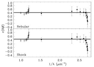
Figure 4: c(H$\beta$) values obtained from different line ratios $vs.$ the inverse of the wavelength in $\mu m$ for the nebular (up) and shock component (down). The filled and non-filled squares correspond to the c(H$\beta$) values derived from Balmer and Paschen lines, respectively. The horizontal line is the weighted average value adopted and the grey band its error

Figure 5: Dereddened fluxes of Balmer (filled squares) and Paschen (non-filled squares) lines to their theoretical flux under the Case B prediction ratio $vs.$ the principal quantum number $n$ for the nebular (up) and shock component (down).

5.2 Comparison of line ratios in the shock and nebular components and the ionization structure

To maximize the shock-to-nebula ratio, the echelle spectra were extracted over the area where the shock component is brighter and the velocity separation with respect to the nebular background gas is maximum (see Figure 2). In Figure 6, we present the weighted average shock-to-nebular ratio for different ionic species, $I$($\lambda$)_sh/$I$($\lambda$)_neb –which was defined in equation (1)– with respect to the ionization potential (IP) needed to create the associated originating ion. In general, as we can see in this figure, the line ratios of the shock component relative to those of the ambient gas are between 1 and 2 for most ionic species with IP above 10 eV, and close to one for the most ionized species as ${\rm O^{2+}}$ and ${\rm Ne^{2+}}$. Since the illumination of the shock should be approximately the same as that of the nebula at this particular zone of the slit, shock-to-nebular ratios of the order of one imply that the shock should be ionization-bounded. This is exactly the opposite situation that Blagrave et al. (2006) find in HH 529, where the shock-to-nebular ratios are clearly lower than 1 indicating that the shock associated to HH 529 is matter-bounded. As we have commented above and can be seen in Figure 6, the shock-to-nebular ratio varies from 1 to 2 for species with an IP higher than 10 eV except in two cases: a) ${\rm Fe^{2+}}$, whose lines show a substantial enhancement in the shock component, probably due to dust destruction (see §5.6), and b) ${\rm Cl^{+}}$, but this can be accidental because this ionic abundance is derived from a single rather faint line with a very large uncertainty. Ionic species with an IP lower than 10 eV show a shock-to-nebular ratio always higher than 2 in Figure 6. In particular, ${\rm Fe^{+}}$, ${\rm Ni^{+}}$ and ${\rm Cr^{+}}$ show ratios larger than 2 and these ions may be also affected by an increase of the gas-phase abundance due to dust destruction. Neutral species like ${\rm O^{0}}$ or ${\rm N^{0}}$ are associated with the presence of an ionization front. In the case of ${\rm O^{0}}$, the shock-to-nebular ratio has been calculated from the [O i] 6300 and 6363 Å lines that are contaminated by telluric emissions but only in the shock component. We extracted the telluric emissions from the zone free of shock emission along the slit and subtracted this feature to the shock component. The shock-to-nebular ratio of [O i] lines is the largest one for those ions which are not heavily affected by possible dust destruction. This is a further indication of the presence of an ionization front in HH 202-S. In the case of [N i] lines, those belonging to the nebular component are also contaminated by telluric emission but, in this case, it was impossible to deblend properly these lines. In Figure 2 we can see the spatio-kinematic profiles of lines of different ionization

Figure 6: Weighted average of shock-to-nebular line ratios $vs.$ the ionization potencial (IP) needed to create the associated originating ion. Non-filled circles correspond to ratios measured from RLs (only for ${\rm O^{+}}$ and ${\rm O^{++}}$). Smaller error bars are of about 3%.

stages of oxygen: ${\rm O^{0}}$, ${\rm O^{+}}$ and ${\rm O^{2+}}$, including RLs and CELs. In the shock component, we can clearly distinguish a stratification in the location of the ions: the bulk of the ${\rm O^{2+}}$ emission is located at the south of the extracted area, ${\rm O^{0}}$ at the north and ${\rm O^{+}}$ is located approximately at the centre of the extracted area. Another interesting feature that can be seen in Figure 2 is that the emissions from RLs and CELs of the same ion seem to show the same spatio-kinematic profiles. These profiles provide further indication that HH 202-S is an ionization-bounded shock. The peak emission of the spatio-kinematic profiles of ions with IP lower or similar to the one of ${\rm O^{+}}$: ${\rm Cr^{+}}$, ${\rm Ni^{+}}$, ${\rm S^{+}}$, ${\rm Fe^{+}}$ or ${\rm H^{+}}$ is located to the north of HH 202-S, as in the case of ${\rm O^{+}}$. Ions as ${\rm He^{+}}$, ${\rm C^{2+}}$ or ${\rm Fe^{2+}}$ show their peak emission about the centre of the aperture, while the ions with the highest IP, as ${\rm Ne^{2+}}$ or ${\rm Ar^{3+}}$, show spatio-kinematic profiles similar to that of ${\rm O^{2+}}$.

5.3 Width of the ionized slab and the physical separation between $\theta^{1}$Ori C and HH 202-S

An interesting result of this paper is the claim that HH 202-S contains an ionization front as we have shown in §4.1 and §5.2. Due to this fact, we can estimate the width of the ionized slab of HH 202-S and its physical separation with respect to the main ionization source of the Trapezium cluster, $\theta^{1}$Ori C. On the one hand, from the maximum emission of the shock component in the spatio-kinematic profiles of ${\rm O^{2+}}$ and ${\rm O^{0}}$ shown in Figure 2, we can measure an angular distance on the plane of the sky of about 3$\aas@@fstack{\prime\prime}$9$\pm$0$\aas@@fstack{\prime\prime}$5. Using the distance to the Orion Nebula obtained by Menten et al. (2007), $d$ = 414$\pm$7 pc, and the inclination angle of HH 202-S with respect to the plane of the sky calculated by O’Dell & Henney (2008), $\theta$ $=$ 48^o, we estimate (11.7$\pm$1.5)$\times$10^-3 pc for the width of the ionized slab. On the other hand, to trap the ionization front in HH 202-S, the incident Lyman continuum flux must be balanced by the recombinations in the ionized slab, $i.e.$,

$$F_{\rm Ly}=\frac{Q(H^{0})}{4\pi D^{2}}=n_{\rm sh}^{2}\alpha_{B}(H^{0},T)L,$$ (11)

where $D$ is the physical separation between HH 202-S and $\theta^{1}$Ori C, $Q(H^{0})$ is the ionizing photon rate, $n_{\rm sh}$ the density in the shock component, $\alpha_{B}(H^{0},T)$ is the case B recombination coefficient for H and $L$ the width of the slab. In order to estimate $Q(H^{0})$, we have used a spectral energy distribution of fastwind code with the stellar parameters for $\theta^{1}$Ori C obtained by Simón-Díaz et al. (2006) –$T_{eff}=39000\pm 1000$ K and log $g=4.1\pm 0.1$ dex– and the distance to the Orion Nebula calculated by Menten et al. (2007). Then, the output parameters have been: the stellar radius $R=(9.0\pm 1.3)R_{\odot}$, the stellar luminosity log $L=38.80\pm 0.14$ dex and the ionizing photon rate $Q(H^{0})=(6.30\pm 2.00)\times 10^{48}$ s^-1. Taking a value for the recombination coefficient, $\alpha_{B}=2.59\times 10^{-13}$ cm^-3 s^-1 at $10^{4}$ K, we have finally calculated a physical separation of $D=0.14\pm 0.05$ pc. This result suggests that HH 202 is quite embedded within the body of the Orion Nebula and, therefore, discarts the origin of the ionized front as result of the interaction of the gas flow with the veil (see §4.1), which is between 1 and 3 pc in front of the Trapezium cluster (see Abel et al., 2004).

5.4 Radial velocity analysis

In Figure 7, we show the average heliocentric velocity of the lines that belong to a given ionic species as a function of the IP needed to create the associated originating ion. We have used two separate graphs to distinguish between the behaviour of the nebular and the shock component. The nebular component shows the typical velocity gradient that has been observed in other positions of the Orion Nebula and other H ii regions (e.g. Bautista & Pradhan, 1998; Esteban & Peimbert, 1999), with a velocity difference of the order of $-$15 km s^-1 between the neutral and the most ionized species. This gradient is likely produced by the presence of flows of ionized gas originating from the ionization front inside the nebula. In contrast, the ions in the shock component show a rather similar radial velocity independently of their IP. This indicates that the bulk of the ionized gas at the HH 202-S is moving at approximately the same velocity with respect to the rest of the nebula. The H i lines (Balmer and Paschen series) of the shock component are shifted by $-$50.7$\pm$1.0 km s^-1 relative to the H i lines of the nebular component and $-$64.8$\pm$1.0 km s^-1 relative to the velocity of the photon dominated region (PDR, +28 km s^-1; Goudis, 1982). The zone covered by our UVES slit (see Figure 1) coincides with position 117$-$256 of Doi et al. (2004). These authors detect two radial velocity components belonging to the shock gas in this zone, a fast component ($-$57 km s^-1) and a slower brighter one ($-$31 km s^-1). Our value of the radial velocity for the shock component of HH 202 ($-$36.8$\pm$1.0 km s^-1) is somewhat more negative than the slower velocity component of Doi et al. (2004), probably our shock component corresponds to the unresolved blend of the two velocity systems detected by those authors.

Figure 7: Heliocentric velocities of the nebular (up) and shock (down) component emission lines $vs.$ the ionization potencial (IP) needed to create the associated originating ion. The velocity of the photon dominated region (dashed horizontal line) is also shown. Non-filled triangles correspond to ions observed in only one kinematic component. Non-filled circles correspond to heliocentric velocities measured from RLs (only for ${\rm O^{+}}$ and ${\rm O^{++}}$).

5.5 The abundance discrepancy and temperature fluctuations

Assuming the validity of the temperature fluctuations paradigm and that this phenomenon produces the abundance discrepancy, we can estimate the values of the $t^{2}$ parameter from the ADFs obtained for each component and ion (see Table LABEL:abioni). In Table LABEL:t2, we include the $t^{2}$ values that produce the agreement between the abundance determinations obtained from CELs and RLs of ${\rm O^{2+}}$ and ${\rm C^{2+}}$. These calculations have been made following the formalism outlined by Peimbert & Costero (1969). Adopting the $t^{2}$ value obtained for ${\rm O^{2+}}$ zone, $t^{2}$(${\rm O^{2+}}$), we have calculated the ionic abundances, the ICFs and the total abundances under the presence of temperature fluctuations and they are presented in Tables LABEL:abioni, LABEL:icf and LABEL:abtot, respectively. As we can see in Table LABEL:abtot, the high $t^{2}$(${\rm O^{2+}}$) value used to derive the abundances for the shock component implies that the total abundances obtained from CELs considering $t^{2}$$>$0 are higher in the shock component than in the nebular one for all the elements. On the other hand, the abundances of C and O obtained from RLs are very similar in both components. Moreover, the O/H ratio computed from CELs for $t^{2}$$>$0 is higher than that obtained from RLs. However, for the nebular component, we find that the total abundance of oxygen determined from CELs considering $t^{2}$$>$0 agrees with the oxygen abundance from RLs. These results can suggest that, perhaps, the $t^{2}$ value we have found for the shock component is too high and, therefore, that the $t^{2}$ paradigm is not applicable in this case. However, we have to consider that we have used a $t^{2}$ value representative of the high ionization zone for all the ions. The increase of the ${\rm O^{+}}$/${\rm O^{2+}}$ ratio in the shock component with respect to the nebular one, due to an enhanced recombination rate, makes the ${\rm O^{+}}$ zone more extended in this component and a lower $t^{2}$(${\rm O^{+}}$) would lead to a better agreement between the O abundances of both components. We have also computed the $t^{2}$ parameter for the ${\rm He^{+}}$ zone using a MLM (see §4.4). The determination of the $t^{2}$(${\rm He^{+}}$) weighs the ${\rm O^{+}}$ and the ${\rm O^{2+}}$ zones depending on their extension. It is remarkable that the $t^{2}$ values obtained from different methods, such as the ${\rm He^{+}}$ lines and the ${\rm ADF(O^{2+})}$, which assume the presence of temperature fluctuations in the observed volume, produce almost identical values in both components, though $t^{2}$(${\rm He^{+}}$) has large uncertainties. These ones can reconcile the total abundances of both components for $t^{2}$$>$0 considering that the MLM depends strongly on the He i 3889 Å line flux and that the shock components of this line and H8 are severely blended. In Table LABEL:t2 we have also included the values of $t^{2}$ obtained by Blagrave et al. (2006) from the ${\rm ADF(O^{2+})}$ that they estimate for the nebular and shock components of HH 529 and those obtained by Esteban et al. (2004) from the ADF of ${\rm O^{2+}}$ and ${\rm C^{2+}}$. The data of Esteban et al. (2004) correspond to a zone free of high velocity flows and can be considered as representative of the nebular component but closer to the Trapezium. The values of the $t^{2}$ obtained for the nebular component of HH 202-S are quite consistent with those obtained by Esteban et al. (2004). The $t^{2}$(${\rm O^{2+}}$) of the nebular component of HH 529 obtained by Blagrave et al. (2006) is lower than the two other determinations, but still consistent with our values within the uncertainties. As has been commented above, the $t^{2}$

^a

Blagrave et al. (2006).

values found in the shock component of HH 202 are much higher than those of the nebular component and the value determined by Blagrave et al. (2006) for the shock component of HH 529. The effect of temperature fluctuations in the spectra of ionized nebulae and their existence has been a controversial problem from the first work of Peimbert (1967). Peimbert (1995), Esteban (2002), Peimbert & Peimbert (2006) have reviewed the possible mechanisms that could produce such temperature fluctuations. Among the possible sources of temperature fluctuations, we can list the deposition of mechanics energy by shocks and the gas compresion due to turbulence. Peimbert et al. (1991) have studied the effect of shock waves in H ii regions using shock models by Hartigan et al. (1987). They found that high $t^{2}$ values can be explained by the presence of shocks with velocities larger than 100 km s^-1. In the case of the flow of 89 km s^-1 that produces HH 202, this effect should produce very small $t^{2}$ values. Therefore, another process or other formalisms of the problem should be taken into account in this case. Further duscussion of this problem is beyond the scope of this article.

5.6 Dust destruction

As indicated in §5.2, the emission lines of refractory elements as Fe, Ni or Cr are much brighter in the gas flow than in the ambient gas. Moreover, the shock component shows relatively bright [Ca ii] lines which are not detected in the spectrum of the ambient gas. On the other hand, in §4.1 we have stated that HH 202-S does not contain a substantial contribution of shock excitation and, therefore, we need other mechanisms to explain those abnormally high line fluxes. It is well known that Fe, Ni, Cr and Ca are expected to be largely depleted in neutral and molecular interstellar clouds as well as in H ii regions. However, theoretical studies have shown that fast shocks –as those typical in HH objects and supernova remnants– should efficiently destroy grains by thermal and nonthermal sputtering in the gas behind the shock front and by grain-grain collisions (McKee et al., 1984; Jones et al., 1994; Mouri & Taniguchi, 2000). Several works have shown that some nonphotoionized HH flows show a decrease in the amount of Fe depletion as determined from the analysis of [Fe ii] lines (Beck-Winchatz et al., 1996; Böhm & Matt, 2001; Nisini et al., 2005). On the other hand, HH 399 is the first precedent of a fully ionized HH object where an overabundance in Fe was detected and this one was related with dust destruction (Rodríguez, 2002). In Table LABEL:depletions we compare the values of the C, O, Fe, Ni and ${\rm Cr^{+}}$ abundances and the Fe/Ni ratios of the Sun (Grevesse et al., 2007) and the nebular and shock components for $t^{2}$$=$0 and $t^{2}$$>$0. In the case of Fe and Ni, we can see that the difference between the abundances of the shock and nebular components are of the order of 0.85 dex for $t^{2}$$=$0 and 1.00 dex for $t^{2}$$>$0. This result indicates that the gas-phase abundance of Fe and Ni increases by a factor between 7 and 10 after the passage of the shock wave. The fact that the Fe/Ni ratio is the same in both components –because the increase of the gas-phase abundance of both elements is the same– and consistent with the solar Fe/Ni ratio within the errors, suggests that the abundance pattern we see in HH 202-S is the likely product of dust destruction. In fact, observations of Galactic interstellar clouds indicate that Fe, Ni –as well as Cr– have the same dust-phase fraction (Savage & Sembach, 1996b; Jones, 2000). It is also remarkable that, although it could be modulated by ionization effects, the behaviour of the ${\rm Cr^{+}}$ abundance is also consistent with the dust destruction scenario. The increase of the ${\rm Cr^{+}}$/${\rm H^{+}}$ ratio between the nebular and shock components is identical to that of Fe and Ni. Considering the solar Fe/H ratio as the reference (12$+$log(Fe$/$H) $=$ 7.45$\pm$0.05, Grevesse et al., 2007) –which is almost identical to the Fe/H ratio determined for the B-type stars of the Orion association (12$+$log(Fe$/$H) $=$ 7.44$\pm$0.04, Przybilla et al., 2008)– we estimate that the Fe dust-phase abundance decreases by about 30% for $t^{2}$$=$0 and about 53% for $t^{2}$$>$0 after the passage of the shock wave in HH 202-S. This result is in good agreement with the predictions of the models of Jones et al. (1994) and Mouri & Taniguchi (2000). In particular, for the velocity determined for HH 202 (89 km s^-1, O’Dell & Henney, 2008), Jones et al. (1994) obtain a level of destruction of iron dust particles of the order of 40%. On the other hand, the Fe gas-phase abundance we measure in HH 202-S follows closely the empirical correlation obtained by Böhm & Matt (2001) from [Fe ii] and [Ca ii] emission line fluxes of several nonphotoionized HH flows. Further evidence that the dust is not completely destroyed in HH 202 is the detection of 11.7 $\mu m$ emission coincident with the bright ionized gas around HH 202-S (Smith et al., 2005). As we can see in Table LABEL:depletions, the depletion factors of Fe and Ni in the nebular component are similar to those found in warm neutral interstellar environments and those at HH 202-S of the order of the depletions observed in the Galactic halo (see Welty et al., 1999, and references therein). In the cases of C and O, the effect of dust destruction in their gas-phase abundance is more difficult to estimate. Firstly, these elements are far less depleted in dust grains than Fe or Ni in neutral interstellar clouds and in H ii regions. Secondly, there is still a controversy about the correct solar abundance of these two elements (see Holweger, 2001; Grevesse et al., 2007). Finally, chemical evolution models predict some increase in the C/H and O/H ratios in the 4.6 Gyr since the formation of the Sun (0.28 and 0.13 dex: Carigi et al., 2005). All these problems make impossible to estimate confident values of the depletion factors for C and O. Considering the data gathered in Table LABEL:depletions, the C abundance is virtually the same in the nebular and shock components, although any possible small difference may be washed out due to the intrinsic relatively large error of the abundance determination of this element. In any case, only a slight increase of the C gas-phase abundance would be expected after the passage of the shock wave for a shock velocity of about 89 km s^-1 (Jones et al., 1994). The uncertainties in the determination of the O abundances are much lower than in the case of C and its determination does not depend on the selection of an appropriate ICF scheme. In Table LABEL:depletions, we see an increase of 0.06 dex in the O abundance in the shock component with respect to the nebular one. These results suggest a possible moderate decrease of the depletion for this element in the shocked material. Very recent detailed determinations of the O abundance of B-type stars in the Orion association (Simón-Díaz, in preparation) indicate that the mean O/H ratio in this zone is 8.76$\pm$0.04. In principle, one would expect that this is a better reference for estimating the dust depletion in the Orion Nebula than the solar one because it corresponds to the $actual$ O abundance at the same location. If we take the B-type stars determination as a reference for the total O/H ratio, the amount of O depletion in the ambient gas would be $-$0.17$\pm$0.06 dex and $-$0.11$\pm$0.06 dex in the gas flow. Therefore, a 30% of the O tied up into dust grains would be destroyed after the passage of the shock front. There are two other alternative methods to estimate the oxygen depletion factor. The first one can be drawn following Esteban et al. (1998). This one is based on the fact that Mg, Si and Fe form molecules with O which are trapped

^a

Grevesse et al. (2007).

in dust grains. We have used Mg, Si and Fe depletions in order to obtain the fraction of O trapped in dust grains. These depletions are estimated considering the Orion gas abundances of Mg and Si given by Esteban et al. (1998), our Fe abundance for $t^{2}$$>$0, the O abundances derived from RLs, the stellar abundances of the Orion association of Si from Simón-Díaz (7.14$\pm$0.10) and Mg and Fe from Przybilla et al. (2008). By assuming that O is trapped in olivine (Mg, Fe)₂SiO₄, pyroxene (Mg, Fe)SiO₃ and several oxides like MgO, Fe₂O₃ and Fe₃O₄ (see Savage & Sembach, 1996a, and references therein), we have estimated an O depletion factor of $-$0.10$\pm$0.04 dex for the nebular component. If we consider the older stellar abundances of Si and Fe from Cunha & Lambert (1994) and the Mg/Fe ratio from Grevesse et al. (2007), this value becomes $-$0.08$\pm$0.05, which is almost identical to that computed from the new stellar Mg, Si and Fe abundances. The last method to obtain O depletion factors assumes that oxygen and iron are destroyed in the same fraction. The fraction of iron dust particules is calculated using the Fe abundances for $t^{2}$$>$0 presented in Table LABEL:depletions and Fe abundance of B-type stars of the Orion association. From this assumption, and taking into account the O abundance from RLs, we have derived a depletion factor of

$-$0.11${}^{+0.11}_{0.14}$ dex in the nebular component. Finally, we have calculated the average of the values obtained from the three methods, finding that the O depletion factor of the ambient gas is $-$0.12$\pm$0.03. In all cases, the depletion becomes larger by about 0.08 dex if we adopt abundances for $t^{2}$=0. Aditionally, the depletion factor in the shock component is smaller than in the ambient gas, probably due to gas destruction.

5.7 Photoionization models for HH 202-S

To test the role of dust destruction both in the temperature structure observed in the shock component and in the iron abundance in the gas, we have run some simple photoionization models for the nebular and the shock components. The models were constructed using Cloudy (Ferland et al., 1998), version 07.02, and assuming a plane-parallel open geometry with density equal to the value adopted from the observations (see Table LABEL:cond). We used a WM-basic (Pauldrach et al., 2001) model stellar atmosphere, with $T_{eff}$ $=$ 39000 K and log $g$ $=$ 4.0, values very similar to those derived by Simón-Díaz et al. (2006) for $\theta^{1}$ Ori C. The number of ionizing photons entering the ionized slab was specified using the ionization parameter, $U$, the ratio of hydrogen-ionizing photons to the hydrogen density. We changed the value of this parameter till the degrees of ionization (given by O⁺/O²⁺) derived for the models were close to the observed ones. The final values used for $U$ imply similar numbers of hydrogen ionizing photons in the nebular and shock models, with a difference of $\sim$40%. We have used the Cloudy “H ii region” abundances, based on the abundances derived by Baldwin et al. (1991), Rubin et al. (1991) and Osterbrock et al. (1992) in the Orion Nebula, for all elements except iron, which we have rescaled in order to reproduce the observed [Fe iii] 4658/H$\beta$ line ratios. The models also have “Orion” type dust: graphite and silicate grains with the Orion size distribution (deficient in small grains, see Baldwin et al., 1991) and an original dust to gas mass ratio of 0.0055. For each model, we used the calculated line intensities to derive the physical conditions and the O⁺ and O²⁺ abundances, following a similar procedure to the one used to derive the observational results. We computed three shock models. Model A has similar characteristics to the nebular model except for the density, and can be used to assess the influence of this parameter on the electron temperatures. Model B has the same input parameters as model A, but with the Fe abundance multiplied by a factor of 7. Model C has the same input parameters as model B but with half the amount of dust. The input model parameters are listed in Table LABEL:models. Table LABEL:constraints shows a comparison for observations and models of the physical conditions, the degree of ionization given by O⁺/O²⁺, and the [Fe iii] 4658/H$\beta$ line ratio. We can see that the nebular model reproduces well the observational constraints. As for the shock models, the increment in the density of model A is enough to explain the temperatures found for the shock component, but does not reproduce the [Fe iii] flux, whereas the higher Fe abundance of model B reproduces well this flux. Model C illustrates that a reduction in the amount of dust does not change significantly the values of the chosen constraints. The introduction of grains smaller than the ones considered in the Orion size distribution of Cloudy will lead to higher temperatures through photoelectric heating, but we do not know what grain size distribution would be suitable for the shock component. The iron abundances in those models that reproduce the observed [Fe iii] line fluxes are somewhat higher than the ones derived from the observations, but they reproduce the value of the shock to nebular abundance ratio. This can be considered a confirmation of the increment in the iron abundance in the shock component, which is most probably due to dust destruction. As it has been discussed in §5.6, dust destruction could also increase the gaseous abundances of other elements like carbon or oxygen and this increment will change the amount of cooling and hence the electron temperature. We ran a model where the abundances of O and C were increased by 14% and found that the derived temperatures decrease by about 200 K.

6 Conclusions

We have obtained deep echelle spectrophotometry of HH 202-S, the brightest knot of the Herbig-Haro object HH 202. Our high-spectral resolution has permitted to separate two kinematic components: the nebular component –associated with the ambient gas– and the shock one –associated with the gas flow. We have detected and measured 360 emission lines of which 352 lines were identified. We have found a clear disagreement between the individual c(H$\beta$) values obtained from different Balmer and Paschen lines. We outline a possible solution for this problem based on the effects of Ly-continuum pumping and l-changing collisions with protons. We have analyzed the ionization structure of HH 202-S concluding that the dominant excitation mechanism in HH 202-S is photoionization. Moreover, the dependence of the $I$($\lambda$)_sh/$I$($\lambda$)_neb ratios and the ionization potential, the comparison of the spatio-kinematic profiles of the emission of different ions, as well as the physical separation estimated of 0.14$\pm$0.05 pc between HH 202-S and $\theta^{1}$Ori C indicate that an ionization front is trapped in HH 202-S due to compression of the ambient gas by the shock. We have derived a high $n_{e}$, about 17000 cm^-3, and similar $T_{e}$ for the low and high ionization zones for the shock component, while for the ambient gas we obtain an $n_{e}$ of about 3000 cm^-3, and a higher $T_{e}$ in the low ionization zone than in the high ionization one. We have estimated that the pre-shock gas in the inmediate vicinity of HH 202 has a density of about 700 cm^-3, indicating that the bulk of the emission of the ambient gas comes from the background behind HH 202. We have derived chemical abundances for several ions and elements from the flux of collisionally excited lines (CELs). In particular, we have determined the ${\rm Ca^{+}}$ and ${\rm Cr^{+}}$ abundances for the first time in the Orion Nebula but only for the shock component. The abundance of ${\rm C^{2+}}$, ${\rm O^{+}}$ and ${\rm O^{2+}}$ have been determined using recombination lines (RLs) for both components. The abundance discrepancy factor for ${\rm O^{2+}}$, ${\rm ADF(O^{2+})}$, is 0.35 dex in the shock component and much lower in the ambient gas component. Assuming that the ADF and temperature fluctuations are related phenomena, we have found a $t^{2}$(${\rm O^{2+}}$) of 0.050 for the shock component and 0.016 for the nebular one. The high $t^{2}$ value of the shock component produces some apparent inconsistencies between the total abundances in both components that cast some doubts on the suitability of the $t^{2}$ paradigm, at least for the shock component. However, the fact that the values of the $t^{2}$ parameter determined from the analysis of the He i line ratios are in complete agreement with those obtained from the ${\rm ADF(O^{2+})}$ supports that paradigm. Finally, the comparison of the abundance patterns of Fe and Ni in the nebular and shock components and the results of photoionzation models of both components indicate that a partial destruction of dust grains has been produced in HH 202-S after the passage of the shock wave. We estimate that the percentage of destruction of iron dust particles is of the order of 30%-50%.

Acknowledgments

We are very grateful to the referee of the paper, J. Bally, for his comments, which have improved the scientific content of the paper. We also thank S. Simón-Díaz for providing us the stellar parameters for $\theta^{1}$ Ori C. This work has been funded by the Spanish Ministerio de Ciencia y Tecnología (MCyT) under project AYA2004-07466 and Ministerio de Educación y Ciencia (MEC) under project AYA2007-63030. V.L. acknownleges support from MEC under project AYA2007-64712. J.G.-R. is supported by a UNAM postdoctoral grant. M.R. acknowledges support from Mexican CONACYT project 50359-F.

References

- Abel et al. (2004) Abel N. P., Brogan C. L., Ferland G. J., O’Dell C. R., Shaw G., Troland T. H., 2004, ApJ, 609, 247
- Baldwin et al. (1991) Baldwin J. A., Ferland G. J., Martin P. G., Corbin M. R., Cota S. A., Peterson B. M., Slettebak A., 1991, ApJ, 374, 580
- Bally et al. (2006) Bally J., Licht D., Smith N., Walawender J., 2006, AJ, 131, 473
- Bally & Reipurth (2001) Bally J., Reipurth B., 2001, ApJ, 546, 299
- Bally & Reipurth (2003) Bally J., Reipurth B., 2003, AJ, 126, 893
- Bautista (2001) Bautista M. A., 2001, A&A, 365, 268
- Bautista (2004) Bautista M. A., 2004, A&A, 420, 763
- Bautista et al. (2008) Bautista M. A., Ballance C., Gull T., Lodders K., Martínez M., Meléndez M., 2008, MNRAS, submitted
- Bautista et al. (1996) Bautista M. A., Peng J., Pradhan A. K., 1996, ApJ, 460, 372
- Bautista & Pradhan (1996) Bautista M. A., Pradhan A. K., 1996, A&AS, 115, 551
- Bautista & Pradhan (1998) Bautista M. A., Pradhan A. K., 1998, ApJ, 492, 650
- Beck-Winchatz et al. (1996) Beck-Winchatz B., Bohm K.-H., Noriega-Crespo A., 1996, AJ, 111, 346
- Benjamin et al. (2002) Benjamin R. A., Skillman E. D., Smits D. P., 2002, ApJ, 569, 288
- Blagrave et al. (2006) Blagrave K. P. M., Martin P. G., Baldwin J. A., 2006, ApJ, 644, 1006
- Blagrave et al. (2007) Blagrave K. P. M., Martin P. G., Rubin R. H., Dufour R. J., Baldwin J. A., Hester J. J., Walter D. K., 2007, ApJ, 655, 299
- Bohlin & Lindler (1992) Bohlin R. C., Lindler D., 1992, STScI Newsletter, 9, 19
- Böhm & Matt (2001) Böhm K.-H., Matt S., 2001, PASP, 113, 158
- Cantó et al. (1980) Cantó J., Goudis C., Johnson P. G., Meaburn J., 1980, A&A, 85, 128
- Carigi et al. (2005) Carigi L., Peimbert M., Esteban C., García-Rojas J., 2005, ApJ, 623, 213
- Cernicharo et al. (1998) Cernicharo J., Lefloch B., Cox P., Cesarsky D., Esteban C., Yusef-Zadeh F., Mendez D. I., Acosta-Pulido J., Lopez R. J. G., Heras A., 1998, Science, 282, 462
- Costero & Peimbert (1970) Costero R., Peimbert M., 1970, Boletin de los Observatorios Tonantzintla y Tacubaya, 5, 229
- Cunha & Lambert (1994) Cunha K., Lambert D. L., 1994, ApJ, 426, 170
- De Robertis et al. (1987) De Robertis M. M., Dufour R. J., Hunt R. W., 1987, J. R. Astron. Soc. Can., 81, 195
- D’Odorico et al. (2000) D’Odorico S., Cristiani S., Dekker H., Hill V., Kaufer A., Kim T., Primas F., 2000, in Bergeron J., ed., SPIE, 4005, p. 121
- Doi et al. (2004) Doi T., O’Dell C. R., Hartigan P., 2004, AJ, 127, 3456
- Esteban (2002) Esteban C., 2002, in Henney W. J., Franco J., Martos M., eds., Revista Mexicana de Astronomia y Astrofisica Conference Series, 12, p. 56
- Esteban & Peimbert (1999) Esteban C., Peimbert M., 1999, A&A, 349, 276
- Esteban et al. (2004) Esteban C., Peimbert M., García-Rojas J., Ruiz M. T., Peimbert A., Rodríguez M., 2004, MNRAS, 355, 229
- Esteban et al. (1998) Esteban C., Peimbert M., Torres-Peimbert S., Escalante V., 1998, MNRAS, 295, 401
- Ferland et al. (1998) Ferland G. J., Korista K. T., Verner D. A., Ferguson J. W., Kingdon J. B., Verner E. M., 1998, PASP, 110, 761
- Froese Fischer & Rubin (2004) Froese Fischer C., Rubin R. H., 2004, MNRAS, 355, 461
- (32) García-Díaz, M. T., Henney, W. J., López, J. A., & Doi, T. 2008, Revista Mexicana de Astronomia y Astrofisica, 44, 181
- García-Rojas & Esteban (2007) García-Rojas J., Esteban C., 2007, ApJ, 670, 457
- García-Rojas et al. (2006) García-Rojas J., Esteban C., Peimbert M., Costado M. T., Rodríguez M., Peimbert A., Ruiz M. T., 2006, MNRAS, 368, 253
- Garnett et al. (1999) Garnett D. R., Shields G. A., Peimbert M., Torres-Peimbert S., Skillman E. D., Dufour R. J., Terlevich E., Terlevich R. J., 1999, ApJ, 513, 168
- Goudis (1982) Goudis C., 1982, The Orion complex: A case study of interstellar matter. Dordrecht. Reidel
- Grandi (1976) Grandi S. A., 1976, ApJ, 206, 658
- Grevesse et al. (2007) Grevesse N., Asplund M., Sauval A. J., 2007, Space Science Reviews, 130, 105
- Hamuy et al. (1994) Hamuy M., Suntzeff N. B., Heathcote S. R., Walker A. R., Gigoux P., Phillips M. M., 1994, PASP, 106, 566
- Hamuy et al. (1992) Hamuy M., Walker A. R., Suntzeff N. B., Gigoux P., Heathcote S. R., Phillips M. M., 1992, PASP, 104, 533
- Hartigan et al. (1987) Hartigan P., Raymond J., Hartmann L., 1987, ApJ, 316, 323
- Henney et al. (2007) Henney W. J., O’Dell C. R., Zapata L. A., García-Díaz M. T., Rodríguez L. F., Robberto M., 2007, AJ, 133, 2192
- Holweger (2001) Holweger H., 2001, in Wimmer-Schweingruber R. F., ed., Solar and Galactic Composition, Springer, Berlin, p. 23
- Johansson et al. (2000) Johansson S., Zethson T., Hartman H., Ekberg J. O., Ishibashi K., Davidson K., Gull T., 2000, A&A, 361, 977
- Jones (2000) Jones A. P., 2000, J. Geophys. Res., 105, 10257
- Jones et al. (1994) Jones A. P., Tielens A. G. G. M., Hollenbach D. J., McKee C. F., 1994, ApJ, 433, 797
- Kingdon & Ferland (1995) Kingdon J., Ferland G. J., 1995, ApJ, 442, 714
- Lucy (1995) Lucy L. B., 1995, A&A, 294, 555
- Luridiana et al. (2009) Luridiana V., Simón-Díaz S., Cerviño M., González Delgado R. M., Porter R. L., Ferland G. J., 2009, ApJ, in press, arXiv:0810.5556
- Martín-Hernández et al. (2002) Martín-Hernández N. L., Peeters E., Morisset C., Tielens A. G. G. M., Cox P., Roelfsema P. R., Baluteau J.-P., Schaerer D., Mathis J. S., Damour F., Churchwell E., Kessler M. F., 2002, A&A, 381, 606
- McKee et al. (1984) McKee C. F., Chernoff D. F., Hollenbach D. J., 1984, in Kessler M. F., Phillips J. P., eds, Galactic and Extragalactic Infrared Spectroscopy. Dordrecht, Reidel, p. 103
- Meaburn (1986) Meaburn J., 1986, A&A, 164, 358
- Meléndez et al. (2007) Meléndez M., Bautista M. A., Badnell N. R., 2007, A&A, 469, 1203
- Mendoza (1983) Mendoza C., 1983, in Flower D. R., ed., Proc. IAU Symp. 103, Planetary Nebulae. D. Reidel Publishing Co., Dordrecht, p. 143
- Menten et al. (2007) Menten K. M., Reid M. J., Forbrich J., Brunthaler A., 2007, A&A, 474, 515