Blow-up in higher-order reaction-diffusion
and wave equations: how $\sqrt{\mbox{log\,log}}$ factor occurs

Abstract.

The origin of non self-similar blow-up in higher-order reaction-diffusion (parabolic) or wave (hyperbolic) equations with typical models

$$\textstyle{u_{t}=u^{2}(-u_{xxxx}+u)\quad\mbox{or}\quad u_{tt}=u^{2}(-u_{xxxx}+u)\quad\mbox{in}\quad(-L,L)\times(0,T),}$$

with zero Dirichlet boundary conditions at $x=\pm L$, where $L>L_{0}\in(\frac{\pi}{2},\pi)$ is discussed. The rate of blow-up is shown to get an extra universal $\sqrt{\ln|\ln(T-t)|}$ factor in addition to the standard similarity one $\frac{1}{\sqrt{T-t}}$. The explanation is based on matching with the so-called logarithmic travelling waves as group invariant solutions of the equation.

Some links and similarities with double-log blow-up terms occurring in earlier studies of plasma physics parabolic equations and the nonlinear critical Schrödinger equation are discussed. On the other hand, $\sqrt{\ln|\ln(T-t)|}$ obtained in Petrovskii’s boundary regularity study for the heat equation in 1934 was the first its appearance in PDE theory.

1. Introduction: THREE mysterious blow-up $\sqrt{\log\,\log}$ of PDE theory

1.1. On our main goal

In the middle of the 1980s, in the study of singularity formation phenomena of blow-up in a reaction-diffusion equation from plasma physics and, almost simultaneously, in self-focusing for the cubic nonlinear Schrödinger equation, the physical and formal asymptotic methods, to say nothing about rigorous justifications, faced an extremely difficult issue of appearance the so-called double logarithmic, or $\sqrt{\log\,\log}$ factor:

(1.1) $$A_{0}(t)\sim\sqrt{\ln|\ln(T-t)|}\quad\mbox{as}\quad t\to T^{-}.$$

Here $T<\infty$ is the blow-up time in the sense that the solution $u=u(x,t)$ of the PDE under consideration is well-defined and is classic for all $t\in(0,T)$, but gets unbounded:

(1.2) $$\textstyle{\lim_{t\to T^{-}}\sup_{x}|u(x,t)|=+\infty.}$$

The goal of this paper is to introduce a number of higher-order scaling invariant nonlinear PDEs of parabolic, hyperbolic, and nonlinear dispersion types, which can exhibit the factor (1.1) in their blow-up behaviour. In fact, we are going to address a wider question:

(1.3) under which assumptions on PDEs, (1.1) occurs in blow-up or not,

and how the absence of (1.1) affects the generic blow-up behaviour. The mysterious (becoming not that much after a proof is found) blow-up factor (1.1) is already well-known for a few PDEs, so we are inevitably obliged to begin with this amazing history of the twentieth century.

1.2. FIRST $\sqrt{\bf log\,log}$ in classic parabolic theory: boundary regularity and Petrovskii’s criterion, 1934

It is truly amazing that its actual origin lies in the heart of PDE theory: regularity of a boundary point. For the Dirichlet problem for the Laplace equation, this study, began by Green, Gauss, Lord Kelvin, Dirichlet in the first half of the nineteenth century and by many other great mathematicians, was completed by Wiener in 1924 [62], who derived his famous regularity criterion (a necessary and sufficient condition). A detailed history of potential theory can be found in Kellogg [31, pp. 277–285].

The same regularity question for the heat equation in a non-cylindrical domain was in 1934 initiated by Petrovskii [47, 48], where the double-log actually occurred for first time. This is the question on irregular or regular point $(x,t)=(0,T)$ for the 1D heat equation

(1.4) $$\left\{\begin{matrix}u_{t}=u_{xx}\quad\mbox{in}\quad Q_{T}=\{|x|<R(t),\,\,\,0<t<T\},\quad\mbox{where}\quad R(t)\to 0^{+}\,\,\mbox{as}\,\,t\to T^{-},\vskip 3.0pt plus 1.0pt minus 1.0pt\vskip 3.0pt plus 1.0pt minus 1.0pt\\ \mbox{with bounded smooth data $u(x,0)=u_{0}(x)$ on $[-R(0),R(0)]$}.\qquad\qquad\qquad\quad\,\,\,\,\,\end{matrix}\right.$$

Here the lateral boundary $\{x=\pm R(t)\}$ is given by a function $R(t)$ that is assumed to be positive and $C^{1}$-smooth for all $0\leq t<T$ and is allowed to have a singularity of $R^{\prime}(t)$ at $t=T^{-}$ only. Then the value of $u(x,t)$ is studied at the end “blow-up” point $(0,T)$, to which the domain $Q_{T}$ “shrinks” as $t\to T^{-}$. Thus, $(x,t)=(0,T)$ is regular, if any value of the solution $u(x,t)$ can be prescribed there by continuity as a standard boundary value on $\partial Q_{T}$. Otherwise the point is irregular, if the value $u(0,T)$ is not arbitrary and is given by the evolution as $t\to T^{-}$.

Petrovskii in 1934–35 [47, 48], in particular, established the following:

(1.5) $$\framebox{$\begin{matrix}{\rm(i)}\,R(t)=2\sqrt{T-t}\,\,\sqrt{\ln|\ln(T-t)|}\quad\Longrightarrow\quad\mbox{$(0,T)$ is regular},\quad\mbox{and}\quad\qquad\quad\vskip 3.0pt plus 1.0pt minus 1.0pt\vskip 3.0pt plus 1.0pt minus 1.0pt\\ {\rm(ii)}\,R(t)=2(1+\varepsilon)\sqrt{T-t}\,\,\sqrt{\ln|\ln(T-t)|},\,\,\varepsilon>0\quad\Longrightarrow\quad\mbox{$(0,T)$ is irregular};\end{matrix}$}$$

see the most recent survey in [25] for a full list of references. As far as we know, (1.5) this is the first clear appearance of the blow-up $\sqrt{\rm log\,log}$ factor in PDE theory.

1.3. SECOND $\sqrt{\bf log\,log}$ in the NLSE (1985): the origin and beginning of the log-log story in nonlinear PDE theory

We now return to the true blow-up problems, but will begin with another famous PDE, which is not a subject of the present paper, but used to be well-recognized as the source of the log-log. It has been well-accepted that the origin (besides Petrovskii’s result more belonging to regularity and even probability theory) of such an unusual rate of blow-up including the $\sqrt{\ln|\ln(T-t)|}$ factor is the nonlinear focusing Schrödinger equation (the NLSE) with the critical exponent

(1.6) $$\textstyle{{\rm i}\,u_{t}=-\Delta u-|u|^{p-1}u\quad\mbox{in}\quad\mathbb{R}^{N}\times(0,T),\quad\mbox{where}\quad p=p_{0}=1+\frac{4}{N},}$$

which is a fundamental model of water wave theory ($N=1$), nonlinear optics (mainly $N=2$), and plasma physics ($N=3$, as a limiting case of Zakharov’s model of Langmuir waves, 1972). It seems that G.M. Fraiman in 1985 [20] (see also [55], and a full history of asymptotics in [57, p. 115]) was the first, who formally derived the log-log correction to the blow-up rate for the cubic case in dimension $N=2$. An alternative way of derivation of the log-log was presented in [35, 43] (1988). See the monograph [57] for a full history and extra details, and [46] for an extended list of further qualitative results. These first results were based on formal ideas saying that the $L^{\infty}$-blow-up rate for some classes of solutions with $L^{2}$-norm slightly above that for the ground state $Q(x)$, satisfies

(1.9) $$\textstyle{\sup_{x}|u(x,t)|\sim\Big{[}\sqrt{\frac{\ln|\ln(T-t)|}{T-t}}\,\,\Big{]}^{\frac{N}{2}}\quad\mbox{as}\quad t\to T^{-}.}$$

We refer to a number of more recent papers, where first qualitative and formal estimates obtained a proper mathematical justification [5, 10, 18, 19, 32, 36, 39, 40, 41, 42, 46, 49, 52]. Many questions remain still open in view of the general complexity of the NLSE (1.6), especially in the multi-dimensional geometry, with $N\geq 2$, where even the representation (1.9) is questionable (other norms can be more appropriate).

In general, blow-up such as (1.9) for the NLSE (1.6) with the strong $L^{2}$-conservation property (the dynamical system being symplectic-Hamiltonian), can be characterized as corresponding to a centre-subspace behaviour relative to the 1D manifold of the rescaled ground states $\{Q_{\omega}(x)\}$, though sometimes this is again not well-understood and questionable (but this is of importance for other models with a different reason for the factor).

1.4. THIRD $\sqrt{\bf log\,log}$: a cubic second-order reaction-diffusion model (1985)

As rather customary in PDE theory, the above log-log factor was almost simultaneously (with Fraiman’s research [20]) detected in reaction-diffusion theory, and was involved into mathematical blow-up area by Friedman and McLeod in 1986 [22], who studied the following parabolic equation from plasma physics:

(1.10) $$\textstyle{u_{t}=u^{2}(u_{xx}+u)\quad\mbox{in}\quad(-L,L)\times(0,T),\quad u(\pm L,t)=0,\quad\mbox{where}\quad L>\frac{\pi}{2}.}$$

More precisely, according to B.C. Low [37], (1.10) can be considered as a model of resistive diffusion of a force-free magnetic field in a plasma. The multi-dimensional version of the model assumes replacing $u_{xx}$ by the Laplacian $\Delta u$. Actually, Low proposed the original nonstationary model, in which a contraction of the magnetic field becomes infinite after a finite time provided that the free-force condition is always satisfied.

It is worth mentioning here that plasma physics with magnetic fields is a permanent source of various reaction-diffusion problems, where evolution of “frozen” magnetic field is typically described by fast-diffusion-like and other quadratic ambipolar mechanisms. For convenience and better understanding a hierarchy of the corresponding parabolic models, we present a typical multi-term RD-type equation for the magnetic field ${\bf B}$ [9]: ${\bf B}_{t}=\nabla\times({\bf v}_{\rm n}\times{\bf B}+{\bf v}_{\rm D}\times{\bf B}-\lambda\nabla\times{\bf B}),$ where $\lambda$ is the ordinary magnetic diffusivity, and ${\bf v}_{\rm D}={\bf v}_{\rm i}-{\bf v}_{\rm n}$ is the drift velocity between ions and neutrals, which is proportional to the Lorentz force, ${\bf v}_{\rm D}\sim\frac{(\nabla\times{\bf B})\times{\bf B}}{4\pi\rho_{\rm i}\nu_{\rm in}}$ (this is the mechanism of cubic nonlinearities). Overall, this yields the following equation:

$$\textstyle{{\bf B}_{t}=\nabla\times\big{[}{\bf v}_{\rm n}\times{\bf B}+\frac{(\nabla\times{\bf B})\cdot{\bf B}}{4\pi\rho_{\rm i}\nu_{\rm in}}\,{\bf B}-(\lambda+\lambda_{\rm AD})\nabla\times{\bf B}\big{]},\quad\mbox{where}\quad\lambda_{\rm AD}=\frac{{\bf B}^{2}}{4\pi\rho_{\rm i}\nu_{\rm in}}}$$

is the ambipolar diffusion coefficient. In addition, there can appear the related 1D complex cubic PDEs of the PME-type (i.e., unlike (1.10), with a divergent diffusion operator) ${\mathcal{B}}_{t}=\big{(}\frac{\mathcal{B}}{2}(|{\mathcal{B}}|^{2})_{z}\big{)}_{z}$ (without ordinary magnetic diffusion, no neutral velocity, and very small ionization fractions), which creates sharp structures in finite time, [9, p. L92].

First qualitative results for (1.10) including conjecture of blow-up were obtained in [60, 61]. On the other hand, (1.10) appears in curve-shortening flows by curvature[3]. Namely, the equation $X_{t}=kN$ of the evolution of a curve $X:S^{1}\times[0,T)\to\mathbb{R}^{2}$ on the plane, where $k$ is the curvature and $N$ is the unit normal, is reduced to

$$k_{t}=k^{2}(k_{\theta\theta}+k)\quad\mbox{on}\quad S^{1}\times(0,T)\quad\big{(}S^{1}=\{0\leq\theta<2\pi\}\,\,\,\mbox{is the unit circle in $\mathbb{R}^{2}$}\big{)}.$$

On derivation, history, blow-up patterns, and other details, see papers [3, 4] to be referred to again. For earlier results and blow-up similarity solutions for such a flow, see e.g., [1].

First, Friedman and McLeod [22, § 2] proved blow-up of solutions if $L>\frac{\pi}{2}$ by using standard at that time barrier and Maximum Principle techniques. Among more delicate results, they proved a rather rare (again at that time) result on the blow-up set of the solution $u(x,t)$:

(1.11) $$B[u_{0}]=\big{\{}x\in(-L,L):\quad\exists\,\,\{x_{n}\}\to x,\,\,\{t_{n}\}\to T^{-}\,\,\mbox{such that}\,\,u(x_{n},t_{n})\to+\infty\big{\}}.$$

By the definition, $B[u_{0}]$ is closed. Then, for smooth symmetric monotone data [22, § 4]

(1.12) $$\textstyle{u_{0}(-x)\equiv u_{0}(x),\quad u_{0}^{\prime}(x)\leq 0\,\,\,\mbox{for}\,\,\,x\geq 0\quad\Longrightarrow\quad B[u_{0}]=[-\frac{\pi}{2},\frac{\pi}{2}].}$$

The next question is then the description of the blow-up behaviour in $B[u_{0}]$ as $t\to T^{-}$, which turns out to be a difficult issue. Namely, the authors showed by some involved mathematics associated with the equivalent integral equation, obtained by dividing by $u^{2}$ and inverting the operator $D_{x}^{2}+I$ on the right-hand side, that the blow-up behaviour does not obey the dimensional similarity law associated with the separation of variables:

(1.13) $$\textstyle{u(x,t)\sim\frac{1}{\sqrt{T-t}}\,\theta(x)\quad\mbox{as}\quad t\to T^{-}\quad\Longrightarrow\quad\frac{1}{2}\,\theta=\theta^{2}(\theta^{\prime\prime}+\theta).}$$

More precisely, unlike (1.13), they showed that the behaviour is governed by the non self-similar law

(1.14) $$\textstyle{u(x,t)\sim\frac{A(t)}{\sqrt{T-t}}\,\cos x,\quad\mbox{where}\quad A(t)\to+\infty\quad\mbox{as}\quad t\to T^{-}.}$$

In addition, it was mentioned on the last page [22, p. 80] that in Watterson’s Thesis in 1985 [60] the (1.1) ansatz was made. An involved proof of (1.1) and the behaviour (1.14) was achieved later on in [4] with a high sharpness: the result therein was

(1.15) $$\textstyle{A(t)=\sqrt{\ln|\ln(T-t)|}(1+o(1))\quad\mbox{as}\quad t\to T^{-}}$$

(we will explain why the multiplier $1\cdot\sqrt{...}$ always occurs all the time here on matching).

It is convenient for further use to discuss the origin of the structure (1.14). The $\cos x$ is obviously a formal stationary solution of (1.10),

(1.16) $$f(x)=\cos x:\quad f_{xx}+f=0,$$

which nevertheless does not satisfy the Dirichlet boundary conditions in (1.10), since $L>\frac{\pi}{2}$. Therefore, (1.14) can be interpreted as an evolution as $t\to T^{-}$ along the 1D manifold $\{\mu\cos x,\,\,\mu>0\}$ of stationary solutions, where the resulting slow-growing factor (1.1) represents a kind of centre manifold (or subspace) behaviour corresponding to the linearized rescaled operator. Of course, the crucial argument establishing (1.1) is fully dependent on the matching of the blow-up structure (1.14) with bounded solutions near $x=\pm L$ through the special behaviour at the localization end points $x=\pm\frac{\pi}{2}$.

1.5. On a “topological” matching: main idea

For further applications to more difficult nonlinear PDEs, we need to explain the qualitative origin of our rather “topological” asymptotic analysis. We claim that the actual origin of the log-log factor (1.1) in the RD model (1.10) can be associated with the existence of the log-travelling wave solutions (log-TW) of the equation (1.10) of the following form

(1.17) $$\textstyle{u_{\rm log}(x,t)=\frac{1}{\sqrt{T-t}}\,g(\eta),\quad\eta=x+\lambda\ln(T-t)\quad(\lambda\not=0).}$$

Substituting (1.17) into (1.10) yields the following ODE:

(1.18) $$\textstyle{\frac{1}{2}\,g-\lambda g^{\prime}=g^{2}(g^{\prime\prime}+g).}$$

These solutions can be obtained as the result of the invariance of (1.10) relative to a one-parameter group of scaling-translating transformations; this was first proved by Ovsiannikov in 1959 [44].

We show that similarity solutions (1.17) play a key role at the end points $x=\pm\frac{\pi}{2}$ of the localization domain $x\in(-\frac{\pi}{2},\frac{\pi}{2})$, and serve as a “transitional mechanism” from the Inner Region-II of bounded solutions for $|x|>\frac{\pi}{2}$ into the internal Inner Region-I $\{|x|<\frac{\pi}{2}\}$ with the blow-up behaviour (1.14). This idea is explained in Figure 1, which will be used in greater detail below. Since in some asymptotic $\eta$-interval, solutions $g(\eta)$ of (1.18) have an extra logarithmic correction in the asymptotics, i.e.,

(1.19) $$g(\eta)\sim(-\eta)\sqrt{\ln(-\eta)}\quad\mbox{for}\quad\eta\ll-1$$

(in this intermediate region, the term $g^{3}$ in (1.18) ought to be neglected), the combination of two logs:

(i) $\sqrt{\ln(-\eta)}$ in (1.19), and

(ii) $\ln(T-t)$ in the $\eta$-variable in (1.17),

lead, on a special formal matching, to the double logs in (1.1) in the RD model (1.10). The later difficult proof such a blow behaviour with the factor (1.1) in Angenent–Velázquez [4] of the behaviour (1.14), (1.1) essentially uses the rescaled variables corresponding to the log-TWs moving frame (1.17) and other related issues.

In what follows, to avoid very complicated technical calculus and further justification (which are actually nonexistent for higher-order PDEs under consideration), we prefer to keep the ideology of the above “topological” matching with a clear geometrical meaning to be explained in Figure 1 in Section 2.

1.6. No log-log for the divergent RD model with finite propagation

The corresponding cubic RD model with the divergent diffusion operator has the form

(1.20) $$u_{t}=(u^{3})_{xx}+u^{3}\quad\mbox{in}\quad\mathbb{R}\times(0,T).$$

Answering the question (1.3), the generic blow-up of nonnegative solutions is then described by the following explicit Zmitrenko–Kurdyumov solution [54]:

(1.21) $$\textstyle{u_{\rm S}(x,t)=\frac{1}{\sqrt{T-t}}\,\theta(x),\quad\mbox{where}\quad\frac{1}{2}\,\theta=(\theta^{3})^{\prime\prime}+\theta^{3}\quad\mbox{in}\quad\mathbb{R},\quad\mbox{so}}$$

(1.22) $$\theta(x)=\left\{\begin{matrix}\frac{\sqrt{3}}{2}\,\cos\big{(}\frac{x}{3}\big{)}\quad\mbox{for}\quad|x|\leq\frac{3\pi}{2},\vskip 3.0pt plus 1.0pt minus 1.0pt\\ \,\,\,\,\,\,\quad 0\quad\qquad\mbox{for}\quad|x|>\frac{3\pi}{2}.\end{matrix}\right.$$

Concerning the asymptotic stability and other generic evolution properties of the particular solution (1.21), see [53, Ch. 4] and references therein. In other words, the weak solution (1.21), (1.22) shows that the blow-up in localized in the domain $(-\frac{3\pi}{2},\frac{3\pi}{2})$, which the heat does not penetrate from for all $t\in(0,T)$. The rate of blow-up in (1.21) is purely self-similar and does not contain any extra log-log or other factors as in (1.1).

Indeed, returning again to (1.3), this absence of the log-log factor can be directly connected with the solvability of the ODE in (1.21), which admits a good weak compactly supported profile $\theta(x)$ given in (1.22). This profile is suitable for both the Cauchy problem in $\mathbb{R}\times(0,T)$ and for the IBVP in $(-L,L)\times(0,T)$ provided that

(1.23) $$\textstyle{L\geq\frac{3\pi}{2}.}$$

If (1.23) is violated, other boundary conditions at the end points $x=\pm\frac{3\pi}{2}$ can be imagined that can lead to extra blow-up factors. Though such posed IBVP for (1.20) are typically looking rather artificial unlike the above and given below more natural parabolic models.

1.7. Main models and results: explaining log-log in higher-order RD models via transition by log-TWs

We claim that the same blow-up factor as in (1.1) exhibits more universality and occurs in other nonlinear scaling-invariant cubic parabolic models of higher-order. Moreover, we also claim that, similar to (1.17),

$$\sqrt{\log\,\log}$$ is generated by the log-TWs transition mechanism.

As a key example, we use the fourth-order RD equation, as a natural extension of (1.10), with zero Dirichlet boundary conditions:

(1.24) $$\left\{\begin{matrix}u_{t}=u^{2}(-u_{xxxx}+u)\quad\mbox{in}\quad(-L,L)\times(0,T),\vskip 3.0pt plus 1.0pt minus 1.0pt\\ u=u_{x}=0\,\,\,\mbox{at}\,\,\,x=\pm L\quad(L>L_{0}).\qquad\quad\,\,\,\end{matrix}\right.$$

Of course, the problem for this higher-order parabolic equation loses any traces of order-preserving, comparison, the Maximum Principle, and barrier features that are always key ingredients in the mathematical study of the second-order parabolic equations. Moreover, even existence-uniqueness results (local) for the degenerate equations such as (1.24) are not properly settled. Nevertheless, we put a blind eye on those difficulties, and concentrate on predicting the log-log factor in the regional blow-up behaviour. Actually, there is some space to avoid such local difficulties: for instance, we can consider uniformly strictly positive solutions with such data on the boundary that the similarity blow-up such as (1.21) is impossible (but then some extra speculations are necessary). For positive solutions $u(x,t)\geq\delta_{0}>0$, classic parabolic theory [16, 21] applies to guarantee local existence and uniqueness of smooth (moreover, analytic) solutions; see a comment at the beginning of Section 2 concerning other weaker solutions $u\geq 0$.

Any rigorous proof of such a blow-up log-log behaviour for (1.24) then becomes rather illusive (e.g., more difficult than for the NLSE (1.6), and any second-order RD-type problem considered before), while formal using of the log-TWs (1.17) is the only source of a proper justification.

In Section 2 we explain the blow-up log-log phenomenon for the model (1.24). In Section 3, we briefly explain how the same factor occurs in the sixth-order parabolic problem

(1.25) $$u_{t}=u^{2}(u_{xxxxxx}+u),\quad u=u_{x}=u_{xx}=0\,\,\,\mbox{at}\,\,\,x=\pm L\quad(L>L_{0}).$$

In Sections 4 and 5, we show that blow-up is simply self-similar for the better divergent models: the fourth-order porous-medium equation with source (the PME–4),

(1.26) $$u_{t}=-(u^{3})_{xxxx}+u^{3},$$

and for the thin film equation with source (the TFE–4)

(1.27) $$u_{t}=-(u^{2}u_{xxx})_{x}+u^{3}.$$

Without loss of generality, for both PDEs (1.26) and (1.27), we consider the Cauchy problem in $\mathbb{R}\times(0,T)$ or the IBVP as in (1.24).

1.8. On extensions to wave and nonlinear dispersion equations

Finally, in Section 6, we show that a similar blow-up log-TW mechanism makes it possible to reconstruct log-log factors for some blow-up patterns for other nonlinear PDEs: for the quasilinear wave equation (the QWE–4)

(1.28) $$u_{tt}=u^{2}(-u_{xxxx}+u),$$

and for the nonlinear dispersion equation (the NDE–3)

(1.29) $$u_{t}=u^{3}(u_{xxx}+u)\quad(\mbox{note ``$u^{3}$" instead of ``$u^{2}$"}).$$

Actually, the formal matching does not change at all in comparison with the parabolic case. Of course, equations (1.28) and (1.29) contain other singularity phenomena such as, in view of nonlinear dispersion mechanisms involved (the local speed of propagation depends on the value of $u$ itself), formation of various shocks, with rather difficult and not fully justified “entropy-like” mathematics (see [23] as a guide for higher-order NDEs and [24] for QWEs–4). We do not take these phenomena into account, and just formally show that there exist some particular blow-up patterns with log-log property, and do not discuss any of their structural stability properties, which can lead to rather obscure mathematics.

1.9. Towards consistency of “topological” matching

As a final comment, the author emphasizes that the non-rigorous and rather rough geometric nature of the presented results makes no problem for him, since, according to his almost thirty years experience in proving various blow-up results, for some of the above higher-order models,

(1.30) $$\framebox{$\begin{matrix}\mbox{proving the proposed blow-up $\sqrt{\ln\,\ln}$ asymptotics}\vskip 3.0pt plus 1.0pt minus 1.0pt\\ \mbox{is not possible in a reasonable finite time.}\end{matrix}$}$$

In fact, it is not that easy even to explain how difficult those problems are. In Section 2.5 we present some operator theory comments, and meantime clarify the above point of view, partially expressed in (1.30), in a more formal but consistent manner, as follows:

(i) It should be noted that the higher-order degenerate singular PDEs such as (1.24), (1.25), (1.27), etc., though having already good and clear applications, have quite obscure local existence-uniqueness-entropy-… theory. The problem is not around blow-up (this can be done rigorously for some classes of solutions), but even small solutions are extremely oscillatory; see similar examples in [17] and [27, Ch. 3-5]. To say nothing about the hyperbolic problem (1.28), which cannot have a smooth local solution at all, since in view of an obvious nonlinear dispersion mechanism, shock (and rarefaction) waves can appear at any suitable point. Note that by no means (1.28) is a (strictly) hyperbolic system with good nowadays entropy theory. Moreover, it can be expected that PDEs such as (1.28) principally cannot have a local uniqueness and well-posedness theory. Similar phenomena of singularity and non-uniqueness exist for (1.29).

(ii) Overall, in general, in view of a complete absence of local existence-uniqueness and entropy theory, studying these higher-order models, we actually deal with huge bundles (so-called, flows in dynamical system theory) of solutions, which can be responsible for various problems settings, from the Cauchy problem up to infinitely many free-boundary problems (FBPs). This is a typical, and unavoidable, feature of modern PDE theory: for equations with non-monotone, non-coercive, non-variational… operators of higher-order, proving existence, uniqueness, entropy, … results along the lines great classic theory from the twenties century is not only very difficult, but can be impossible in principle.

(iii) Therefore, dealing with bundles (flows) of blow-up solutions, we propose a rather rough asymptotic method, which, as must be admitted, does not specify many particular features of solutions involved, but is able to detect some universal property of $\log\log$-factor, which holds for all such blow-up ones, regardless which problems (Cauchy, FBPs, Neumann, Robin, Florin, Stefan,…) are posed. Further refining of the asymptotic method, will require a sharper posing of the Cauchy or FBPs, i.e., matching with boundary behaviour, which is completely different (e.g., extremely oscillatory) for various problems. Inevitably, one faces difficult local existence/uniqueness/entropy/etc. aspects that are unclear for the most of models, which cannot be a subject of a single paper.

(iv) In a natural sense, the proposed (“topological”, but very rough, if you wish) matching well corresponds to common understanding coming from the theory of asymptotic series, which are not converging but first terms correctly describe the behaviour of the functions relative to a small parameter $\varepsilon\to 0$. From planetary motion study in the seventeenth century (Newton-Halley’s period), it is known that taking many terms of asymptotic expansion gives worse results, while first terms are sufficient to predict the behaviour. In a certain sense, a similar asymptotic phenomenon happens in our study: trying to improve the expansion, we involve extra, highly oscillatory and singular terms, which are deeper connected with the whole solution bundle that we are not unaware of.

(v) Thus, even in the clear presence of a certain fear of a justified criticism from the attentive Readers, the author prefers to keep the style of the asymptotic analysis more based on a topological matching, rather than a traditional metric one, where all the terms are carefully estimated to convince. Of course, a standard balancing of all the differential terms can be done for all the higher-order models, but not more than that: any further refining the expansion enters the oscillatory-singular solution bundles and any meaning and significance of the blow-up expansion will be lost and become illusive.

2. How log-TWs imply the log-log blow-up factor

Thus, we fix the model (1.24) as the basic one for explaining the occurrence of the log-log factor (1.1) in the generic blow-up. Concerning questions of existence and uniqueness of solutions of such higher-order equations, we refer to the pioneering paper by Bernis and Friedman [7], where a general approach to constructing such nonnegative solutions has been developed. Clearly, their methods of “singular parabolic $\varepsilon$-regularizations” for constructing non-negative solutions of the Cauchy problem or free-boundary problems (depending on parameters) apply to a very wide class of equations including (1.24), (1.25), and many others, linear or nonlinear. On the other hand, for a number of higher-order parabolic equations, proper solutions of the Cauchy problem can be oscillatory and of changing sign (see [8, 17], [27, p. 152] and references therein), but these local interface aspects can be neglected at this stage while dealing with peculiar properties of blow-up of very large solutions.

2.1. On nonexistence of blow-up separable-variable solutions

Bearing in mind (1.3), this is the first crucial step of any blow-up study. Thus, we look for the standard self-similar blow-up for (1.24) in the form as in (1.21),

(2.1) $$\textstyle{u_{\rm S}(x,t)=\frac{1}{\sqrt{T-t}}\,\theta(x),\quad\mbox{where}\quad\frac{1}{2}\,\theta=\theta^{2}(-\theta^{(4)}+\theta).}$$

Recall that we consider either the Cauchy problem for the equation in (1.24), so we demand a localized patter satisfying

(2.2) $$\theta(x)\to 0\quad\mbox{as}\quad x\to\pm\infty,$$

or the IBVP as in (1.24), i.e., one needs a proper solution $\theta(x)$ such that

(2.3) $$\theta=\theta^{\prime}=0\quad\mbox{at}\quad x=\pm L.$$

It is easy to see that such solutions of the ODE in (2.1) do not exist. Dividing the ODE by $\theta^{2}$, multiplying by $\theta^{\prime}$, and integrating by parts yields

(2.4) $$\textstyle{\frac{1}{2}\,\ln|\theta|=-\theta^{\prime\prime\prime}\theta+\frac{1}{2}\,(\theta^{\prime\prime})^{2}+\frac{1}{2}\,\theta^{2}+C,}$$

where $C\in\mathbb{R}$ is a constant of integration. This identity is true in the standard classic sense for smooth positive solutions $\theta(x)>0$, and also remains valid for a proper class of solutions of changing sign having sufficiently regular zeros (this is a question of a suitable functional setting, not accented here). We fix this negative result:

Proposition 2.1.

The identity $\eqref{p7}$ does not allow nontrivial sufficiently smooth, bounded, and vanishing solutions $\theta(x)$ satisfying $\eqref{p5}$ or $\eqref{p6}$.

This negative result can be associated with some king of a strong local monotonicity of a nonlinear elliptic operator induced by the equation in (2.1).

2.2. On self-similar blow-up for the Neumann or periodic problem

Note that, for the Neumann conditions for the IBVP,

(2.5) $$\theta^{\prime\prime}=\theta^{\prime\prime\prime}=0\quad\mbox{at}\quad x=\pm L,$$

the ODE in (2.1) can admit a good proper solution $\theta(x)$, and then the blow-up becomes purely self-similar as in (2.1). The same can occur for the periodic problem:

(2.6) $$\theta(-L)=\theta(L),\quad\theta^{\prime}(-L)=\theta^{\prime}(L),\quad\theta^{\prime\prime}(-L)=\theta^{\prime\prime}(L),\quad\theta^{\prime\prime\prime}(-L)=\theta^{\prime\prime\prime}(L).$$

We arrive at the problem of asymptotic structural stability of $th$ as $t\to T^{-}$, which can be solved in a standard manner by considering the rescaled equation for the rescaled solution:

(2.7) $$\textstyle{v(x,\tau)=\sqrt{T-t}\,u(x,t),\,\,\,\tau=-\ln(T-t)\quad\Longrightarrow\quad\framebox{$v_{\tau}=v^{2}(-v_{xxxx}+v)-\frac{1}{2}\,v.$}}$$

It is key that (2.7) is a gradient dynamical system with the Lyapunov function

(2.8) $$\textstyle{\frac{\mathrm{d}}{{\mathrm{d}}\tau}\big{[}\frac{1}{2}\int(v_{xx})^{2}-\frac{1}{2}\int v^{2}+\frac{1}{2}\int\ln|v|\big{]}=-\int\frac{(v_{\tau})^{2}}{v^{2}}\leq 0.}$$

As in standard blow-up theory, the main difficulty in proving the stabilization as $\tau\to+\infty$ in the rescaled PDE (2.7) will be a priori bounds on the orbit, i.e., that

(2.9) $$\textstyle{|v(x,\tau)|\leq C\quad\mbox{and}\quad\sup_{x}|v(x,\tau)|\not\to 0\quad\mbox{as}\quad\tau\to+\infty.}$$

Then, if the set of solution of the ODE (2.1), (2.5) or (2.6) is discrete, then there exists a unique stationary profile $\theta(x)$ such that

(2.10) $$v(x,\tau)\to\theta(x)\quad\mbox{as}\quad\tau\to+\infty,$$

in a suitable metric (e.g., uniformly for strictly positive and hence classic solutions).

Finally, let us notice that the solvability and multiplicity for the Neumann problem (2.5) or a periodic one (2.6) are not easy (though the variational structure suggests existence of many periodic solutions), essentially depends on the length parameter $L$, and can deliver some striking surprises.

2.3. Stationary profiles and a bound on $L$

Thus, assuming that a standard separable blow-up solution does not exist, we then ought to find the stationary one (cf. (1.16)),

(2.11) $$f(x):\quad-f^{(4)}+f=0\quad\mbox{on}\quad(-L_{0},L_{0}),\quad f=f^{\prime}=0\quad\mbox{at}\quad x=\pm L_{0}.$$

Looking for an even profile, we set ($L$ denotes $L_{0}$)

(2.12) $$f(x)=\cos x+C\cosh x\quad\Longrightarrow\quad\left\{\begin{matrix}\cos L=-C\cosh L,\vskip 3.0pt plus 1.0pt minus 1.0pt\\ \sin L=C\sinh L,\,\,\,\,\end{matrix}\right.\quad\mbox{or}\quad\tan L=-\tanh L.$$

The last algebraic equation yields the first positive root $L_{0}\in(\frac{\pi}{2},\pi)$, which is taken into account in the statement (1.24) in order to avoid existence of classic stationary solutions and hence no blow-up.

2.4. Formal matching with log-TW behaviour: a “topology” approach

Thus, assuming that $L>L_{0}$, similar to (1.14), we suggest that the blow-up evolution is close to the manifold of stationary solutions, i.e., we study the solutions with the behaviour

(2.13) $$\textstyle{u(x,t)\sim\frac{A(t)}{\sqrt{T-t}}\,f(x),}$$

where $f(x)$ is a stationary solution given by (2.12) normalized by its value at the origin,

(2.14) $$f(0)=1+C\quad(C>0).$$

The further strategy of matching is explained in Figure 1, which suggests to match the Inner Region-I with the strong and fast blow-up asymptotics (2.13) with the log-TW Inner Region-II situated close to the end point $x=L_{0}$ (we consider the $x$-symmetry geometry).

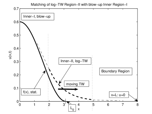
Figure 1. On the idea of a schematic “topological” matching of two Inner Regions.

We are assuming that in Region-II, the solutions are sufficiently small, so we take into account the diffusion-like operator only,

(2.15) $$u_{t}=-u^{2}u_{xxxx}\quad(x\approx L_{0}).$$

Then, taking the log-TW (1.17) yields the following ODE:

(2.16) $$\textstyle{\frac{1}{2}\,g-\lambda g^{\prime}=-g^{2}g^{(4)}.}$$

It is now key that the ODE (2.16) admits the following asymptotics:

(2.17) $$\textstyle{g(y)=(-y)^{2}\sqrt{\ln(-y)}(1+o(1))\quad\mbox{as}\quad y\to-\infty.}$$

Actually, the leading quadratic behaviour $\sim y^{2}$ well corresponds to the quadratic “boundary layer” with the stationary structure

(2.18) $$f(x)=C_{1}(L_{0}-x)^{2}(1+o(1))\quad\mbox{as}\quad x\to L_{0}^{-}\quad(C_{1}>0).$$

The logarithmic correction in (2.17) has the same type as in (1.19), so it is supposed to generate the same log-log factor as in (1.1).

More precisely, according to (1.17), we need to match the behaviour in Region-II,

(2.19) $$\textstyle{u(x,t)\sim\frac{1}{\sqrt{T-t}}\,\big{[}-x-\lambda\ln(T-t)\big{]}^{2}\,\sqrt{\ln(-x-\lambda\ln(T-t))},}$$

with that in blow-up Region-I, where, by the assumption (2.13), the following holds:

(2.20) $$\textstyle{u(x,t)\sim\frac{A(t)}{\sqrt{T-t}}\,C_{1}(x-L_{0})^{2}\quad\mbox{for}\quad x\approx L_{0}^{-}.}$$

Note that the expansion (2.19) should be treated as already the extended one from the corresponding asymptotic region. A more detailed expansion for smaller values of $u$ will be inevitably affected by the singular and oscillatory behaviour of solutions close to $x=L_{0}$ and $x=L$, which we would like to avoid at this stage and refer to the discussion in Section 1.9. More definitely, the expansion (2.19) up to some admissible perturbations (and partially (2.20), which is more regular) precisely defines the required class of solutions of the IBVP or any of FBP problems. Of course, there are other solutions of the PDE under consideration with a completely different blow-up behaviour having nothing to do with a double-log factors.

We omit at this moment the necessary (delicate and questionable) stage in matching, where a suitable time-dependence of the log-velocity $\lambda=\lambda(t)$ is assumed, [53, p. 308]. Currently, as usual in matching concepts and theory, two manifolds of solutions such as (2.19) and (2.20) admit matching if the corresponding pairs of leading multipliers are overlapping at some intermediate values of $x$, possibly, different for both pares. One can object that the log-TW expansion in (2.19) describes moving wave (see the arrow in Figure 1), unlike the standing one in (2.20), which, at the first sight, makes matching rather suspicious. We should mention in connection with that the log-TW in Region-II moves with the logarithmic speed $\sim|\ln(T-t)|$, i.e., very slow in comparison with the power rate $\sim\frac{1}{\sqrt{T-t}}$ of the blow-up divergence in Region-I. In other words, relatively, this can be classified as an effectively standing wave, which makes the matching correct and possible after necessary extra arguments.

Again carefully looking at the manifolds (2.19) and (2.20), we see that the two pairs of different multipliers that are, as $t\to T^{-}$,

(2.21) $$\framebox{$(-x-\lambda\ln(T-t))^{2}\,\,\&\,\,(x-L_{0})^{2}$}\,\,\,\mbox{and}\,\,\,\framebox{$\frac{1}{\sqrt{T-t}}\,\sqrt{\ln(-x-\lambda\ln(T-t))}\,\,\&\,\,\frac{A(t)}{\sqrt{T-t}},$}$$

admit natural “structural matching” on some compact subsets (different for both) in $x$. Actually, according to typical concepts of asymptotic analysis, one needs to observe and to get “similar geometric forms” in space and time of matched flows. This can be definitely done for the pairs in (2.21), where the first pair of space distributions are both similar and quadratic, while the second pair assumes to be similar for some special functions $A(t)$ only. We must admit again that by no means our goal is to prove this matching rigorously (whatever “proof” means).

Then setting $x\approx L_{0}$ in the second pair leads to the conclusion (1.1): as $t\to T^{-}$,

(2.22) $$\textstyle{\framebox{$\frac{1}{\sqrt{T-t}}\,\sqrt{\ln(-\lambda\ln(T-t))}\sim\frac{A(t)}{\sqrt{T-t}}$}\quad\Longrightarrow\quad A(t)\sim\sqrt{\ln|\ln(T-t)|}(1+o(1)).}$$

Note that $\lambda$ even being a slow growing function completely disappears in this matching, so even this rough accuracy guarantees the coefficient “1” (and $\lambda=\lambda(t)$ is contained in the $o(1)$-term only, which is not of importance).

2.5. On some standard metric estimates and operator balance: the origin of principal difficulties

Let us return to a more mathematical (rather than geometrical)) PDE meaning of these speculations. In fact, this suffices to balance differential terms and perturbations in the rescaled equation for $v$ in (2.7), where $\tau=-\ln(T-t)\to+\infty$ as $t\to T^{-}$. Actually, Figure 1 is more suitable for the rescaled function $v(x,\tau)$, which is expected to have a slow logarithmic growth as $\tau\to+\infty$ unlike the fast algebraic one for $u(x,t)$ as $t\to T^{-}$. We next need to rescale as in (2.7) the asymptotic flows (2.19) and (2.20), etc.

We begin with a standard approach to such a matching by starting with the inner R-I rescaled expansion (2.19), i.e., $v(x,\tau)\sim A(\tau)f(x)$, which naturally require introducing the new variable $w$ and the corresponding rescaled equation:

(2.23) $$\left\{\begin{matrix}v(x,\tau)=A(\tau)w(x,\tau)\quad\mbox{and}\quad A^{2}(\tau)\,{\mathrm{d}}\tau={\mathrm{d}}s,\vskip 3.0pt plus 1.0pt minus 1.0pt\\ w_{s}=w^{2}(-w_{xxxx}+w)+\frac{1}{2A^{2}(\tau)}\,w-\frac{A^{\prime}(\tau)}{A^{3}(\tau)}\,w.\,\,\end{matrix}\right.$$

Thus, here $A(\tau)$ is unknown, but (1.1) suggests that

(2.24) $$\textstyle{A(\tau)\sim\sqrt{\ln\tau}\quad\mbox{and}\quad s\sim\tau\ln\tau\,\,\,\big{(}\tau\sim\frac{s}{\ln s}\big{)}\quad\mbox{as}\quad\tau\to+\infty\quad(\mbox{expectation}).}$$

Indeed, the perturbed equation (2.23) with the leading (by (1.1)) perturbation $\sim O\big{(}\frac{1}{A^{2}(\tau)})$ describes the stabilization to the stationary profile:

(2.25) $$w(x,\tau)\to f(x)\quad\mbox{as}\quad\tau\to+\infty,\quad\mbox{where}\quad f(x)\,\,\mbox{solves (\ref{13})},$$

on compact subsets in $[0,L_{0})$. Note that, for the desired result (2.24), the following holds:

(2.26) $$\textstyle{\frac{1}{A^{2}(\tau)}\sim\frac{1}{\ln\tau}\not\in L^{1}_{s}((1,\infty)),\quad\mbox{since}\quad\frac{{\mathrm{d}}s}{A^{2}(\tau)}\sim{\mathrm{d}}\tau,}$$

i.e., the perturbation is not integrable in $L^{1}$ that causes extra difficulties (though is a typical feature of many blow-up and extinction problems, [28]). However, this stage of the analysis is rather standard, since the unperturbed equation

(2.27) $$w_{s}=w^{2}(-w_{xxxx}+w)$$

is a gradient system (cf. (2.8)), though fighting the perturbation terms in (2.23) can be rather technical (but hopefully not of a principle issue). In standard blow-up theory such problems are tackled by theorems on stability of $\omega$-limit sets with respect to arbitrary small perturbations of the dynamical system, provided that the unperturbed problem is uniformly Lyapunov stable; see examples and a large number of references in [28].

Anyway, this is not the case, where the main difficulty occur. Namely, we need to match the behaviour (2.23), (2.25) with that corresponding to a proper one induced by the boundary conditions at $x=L$ (or an FBP setting, which is hard to distinguish from). Then we ought to perform the linearization:

(2.28) $$\textstyle{w(x,s)=f(x)+Y(x,s)\quad\Longrightarrow\quad Y_{s}={\bf C}Y+2fY(-Y^{(4)}+Y)+\frac{1}{2A^{2}}\,f+...\,,}$$

where we omit all asymptotically smaller linear and nonlinear terms, which however can be important for matching. As usual, equation in (2.28) clearly shows that full spectral theory of the linearized operator

(2.29) $${\bf C}=f^{2}(x)(-D^{4}_{x}+I)\quad\mbox{in}\quad x\in[0,L_{0})$$

is necessary for extension of the solution for $x\geq L_{0}$. Fortunately, it is symmetric in the weighted space $L^{2}_{\rho}$, with the weight $\rho=f^{-2}(x)\geq 0$, which is singular at the end point $x=L_{0}$. However, checking the crucial end point $x=L_{0}$ and using the asymptotics of the coefficient (2.18), yields Euler’s equation in the spectral problem:

(2.30) $$C_{1}^{2}(L_{0}-x)^{4}(-\psi^{(4)}+\psi)+...=\lambda\psi.$$

Hence, linearly independent solutions polynomial with the characteristic equation:

(2.31) $$\psi(x)\sim(L_{0}-x)^{m}\quad\Longrightarrow\quad C_{1}^{2}m(m-1)(m-2)(m-3)+\lambda=0.$$

This shows that the necessary spectral theory, though covered by classic theory of singular ordinary differential operators (see, e.g., Naimark [38]), can be rather tricky. In particular, deficiency indices of the operator (2.29) are not easy to detect in $L^{2}_{\rho}$. More precisely, depending on the boundary matching, this can require self-adjoint extensions in both the cases of discrete and continuous spectra. Infinitely oscillatory behaviour for complex values of $m=a+{\rm i}\,b\in{\mathbb{C}}$ in (2.31) ($\lambda$ remains real) occurs close to $L_{0}^{-}$, where

(2.32) $$Y(x,s)\sim{\mathrm{e}}^{\lambda s}(L_{0}-x)^{a}\sin(b\ln(L_{0}-x))\quad\mbox{as}\quad s\to+\infty;$$

cf. the discussion of oscillatory issues in Section 1.9. Thus, using proper spectra theory of (2.29) with eigenfunction expansions of $w(x,s)$ of (2.28) over a discrete (better) or continuous (most plausible for many problem settings) is the first key concern here.

Continuing the spectral aspects of the expansion, we next assume that the spectrum of ${\bf C}$ in (2.29) is continuous in a suitable setting and deficiency indices, so we may impose the following behaviour of the solution $Y$ of (2.28):

(2.33) $$Y(x,s)=\mu(s)\Phi(x)+...\quad\mbox{as}\quad s\to+\infty.$$

Substituting this into (2.28) and naturally assuming that

(2.34) $$\textstyle{\mu^{\prime}_{s}=\mu^{\prime}_{\tau}\tau^{\prime}_{s}\equiv-\frac{A^{\prime}}{A^{5}}\quad\Longrightarrow\quad|\mu^{\prime}(s)|\ll|\mu(s)|\quad\mbox{for}\quad s\gg 1}$$

(this is true for the expectation (2.24)), we arrive at the following first rough balance:

(2.35) $$\textstyle{\mu^{\prime}_{s}\Phi=\mu{\bf C}\Phi+\frac{1}{2A^{2}}f+...\quad\Longrightarrow\quad\mu(s)=\frac{1}{2A^{2}(\tau)}\quad\mbox{and}\quad{\bf C}\Phi+f=0.}$$

Again, a suitable solvability of the $\Phi$-equation in (2.35) requires posing proper boundary conditions at the singular end-point $x=L_{0}$ and satisfactory spectral theory of ${\bf C}$.

Meantime, we solve the ODE for $\Phi$ in (2.35) close to the singular end-point $x=L_{0}$:

(2.36) $$\textstyle{-\Phi^{(4)}+\Phi=-\frac{1}{f(x)}=-\frac{1+o(1)}{C_{1}(L_{0}-x)^{2}}\quad\mbox{as}\quad x\to L_{0}^{-}.}$$

This yields the following non-regular asymptotic expansion:

(2.37) $$\textstyle{\Phi(x)=-\frac{1}{2C_{1}}\,z^{2}\ln z+A_{1}+A_{2}z+A_{3}z^{2}+A_{4}z^{3}+...\quad\mbox{as}\quad z=L_{0}-x\to 0^{+}.}$$

Here we see the first clear appearance of the $\ln(L_{0}-x)$ in the framework of this standard matching and operator analysis:

(2.38) $$\textstyle{\Phi(x)\sim-\frac{1}{2C_{1}}\,(L_{0}-x)^{2}\ln(L_{0}-x)+A_{1}+A_{2}(L_{0}-x)+...\quad\mbox{as}\quad x\to L_{0}^{-},}$$

which is indeed a reliable remnant of the asymptotic expansion (2.17) for the log-TW profile $g(y)$ satisfying (2.16). The integration constants $A_{1,2,3,4}\in\mathbb{R}$ in (2.37) should be obtained by further matching (some of them can be arbitrary and depend on initial data).

Next, in the R-II, where $w$ is uniformly small and hence $w^{3}$ can be neglected, the problem (2.23), with the behaviour (2.33) at the end-point $x=L_{0}$, takes the form

(2.39) $$\left\{\begin{matrix}w_{s}=-w^{2}w_{xxxx}+\mu(s)w+...\quad\mbox{in}\quad(L_{0},L)\times\mathbb{R}_{+},\qquad\qquad\,\,\vskip 3.0pt plus 1.0pt minus 1.0pt\\ w=A_{1}\mu(s),\,\,w_{x}=-A_{2}\mu(s),\,\,x=L_{0};\quad w=w_{x}=0,\,\,x=L.\end{matrix}\right.$$

The precise behaviour of $w$ and the derivatives $w_{x}$ and $w_{xx}$ at $x=L_{0}$ is defined by (2.33). Therefore, we add to (2.39) the following overdetermining condition

(2.40) $$\textstyle{w_{xx}(x,s)=-\frac{1}{C_{1}}\ln(x-L_{0})(1+o(1))\mu(s)\quad\mbox{as}\quad x\to L_{0}^{+},}$$

which is expected to detect the unknown function $A(\tau)$. Theoretically, once these have been achieved, extending the solution up to the original boundary point $x=L$ will define the necessary ODE-type equation for the unknown function $A(\tau)$ such as, very roughly,

(2.41) $$A^{\prime}\sim{\mathrm{e}}^{-A^{2}}\quad\Longrightarrow\quad A(\tau)\sim\sqrt{\ln\tau}\quad\mbox{for}\quad\tau\gg 1.$$

The principle key difficulties start now, when we arrive at the problem (2.39). The point is that when $w(s,x)$ approaches 0, the problem becomes extremely sensitive and demand solving a number of linear and nonlinear eigenvalue problems, where we face in a full scale those unresolved local existence-uniqueness-entropy-etc. problems mentioned in Section 1.9. Namely, even the unperturbed problem

(2.42) $$w_{s}=-w^{2}w_{xxxx}\quad\mbox{on small solutions}\quad|w|\ll 1$$

is not well-understood at all. Note that the second-order counterpart of (1.10),

(2.43) $$w_{s}=w^{2}w_{xx},$$

is also not easy, but by a contact Bäcklund symmetry reduces to the heat equation:

(2.44) $$\textstyle{v_{s}=v_{yy},\quad\mbox{where}\quad w(x,s)=\frac{1}{\phi_{x}(x,s)}\quad\mbox{and}\quad\left\{\begin{matrix}y=\phi,\qquad\\ x=v(y,s);\end{matrix}\right.}$$

see [53, p. 78] and references therein. Actually, such a homology (2.43) $\mapsto$ (2.44) eventually creates a relation (2.41), where the exponential term ${\mathrm{e}}^{-A^{2}}$ is naturally associated with the Gaussian fundamental solution of the operator $D_{s}-D^{2}_{y}$ in (2.44). Obviously, no such nonlocal symmetry is available for the much more difficult PDE (2.42).

Thus, the technicalities at this last stage are extremal and which deserves extra special difficult analysis that we cannot be performed in the present more formal paper (will require at least an extra dozen of sheets of hard calculations), so that, mathematically:

Main difficulty: problems (2.39) and (2.42) are not doable at the moment

(an open problem for the attentive Reader). Let us note that spectral theory of generalized fourth-order non-symmetric Hermite operators (an operator pair) [15] can be key:

(2.45) $$\left\{\begin{matrix}{\bf B}=-D_{y}^{4}+\frac{1}{4}\,yD_{y}+\frac{1}{4}\,I,\vskip 3.0pt plus 1.0pt minus 1.0pt\\ {\bf B}^{*}=-D_{y}^{4}-\frac{1}{4}\,yD_{y}\qquad\,\,\end{matrix}\right.\quad\Longrightarrow\quad\textstyle{\sigma({\bf B})=\sigma({\bf B}^{*})=\big{\{}\lambda_{k}=-\frac{k}{4},\,k\geq 0\big{\}}.}$$

As we have mentioned, exactly in this R-II, a delicate and specially deformed structure of log-TWs are crucial for creating the whole pattern. Thus, the geometric approach of formal matching makes it possible to avoid some (too) detailed refinement of the solution expansion, and establishes that the double-log factor can occur for a kind of an “envelope” of a wide class of blow-up solutions induced by various functional settings. However, the behaviour is expected to be so difficult that we will not be surprised (e.g.,) if the resulting more correct calculation provides us with a different double-log factor $\hat{A}(t)\sim\big{[}\ln|\ln(T-t)|\big{]}^{3/4}$ instead of the standard one (1.1), though the topology matching via (2.21), (2.22) indicates that this is not the case.

Finally, let us point out again that a full (formal) asymptotic expansion technique also assumes the next matching of the log-TW Region-II with the Boundary one close to $x=L$, where another (and hopefully and typically much weaker than at $x=L_{0}$) boundary layer of uniformly bounded solutions can occur. As usual, this is expected to be easier (and less principal), but can be also tricky, as everything concerning such nonlinear degenerate higher-order operators. We recall that a proper and mathematically justified matching of those manifolds of solutions via rigorous compactness-like arguments seems not achievable for the higher-order parabolic equations under consideration. Note again that the analysis in [4] for (1.10) was essentially and inevitably based, among others, on Maximum and Comparison Principle arguments, which are non-existent for higher-order parabolic flows. Moreover, as we have pointed out in greater detail in Section 1.9, the CP, IBVP, or any FBP settings for (1.24) have not been well developed still, so we have to be very careful in deriving asymptotic blow-up properties of some possibly nonexistent and/or non-unique solutions.

3. Briefly on the sixth-order model: the log-log universality

For the equation (1.25), the ODE in (2.1) is

(3.1) $$\textstyle{\frac{1}{2}\,\theta=\theta^{2}(\theta^{(6)}+\theta),}$$

so that nonexistence of a sufficiently smooth solution follows from the identity (cf. (2.4))

(3.2) $$\textstyle{\frac{1}{2}\ln|\theta|=\theta^{(5)}\theta^{\prime}-\theta^{(4)}\theta^{\prime\prime}+\frac{1}{2}\,(\theta^{\prime\prime})^{2}+\frac{1}{2}\,\theta^{2}+C.}$$

The ODE for the log-TWs in Inner Region-II now takes the form

(3.3) $$\textstyle{\frac{1}{2}\,g=g^{2}g^{(6)}+...\quad\Longrightarrow\quad g(\eta)\sim\frac{1}{2\sqrt{3}}\,(-\eta)^{3}\sqrt{\ln(-\eta)}\quad\mbox{as}\quad\eta\to-\infty.}$$

Therefore, the same argument of matching with the stationary structure in blow-up Inner Region-I governed by

(3.4) $$f(x):\quad f^{(6)}+f=0\quad\mbox{in}\quad(-L_{0},L_{0}),\quad f=f^{\prime}=f^{\prime\prime}=0\,\,\,\mbox{at}\,\,\,x=\pm L_{0}$$

(hence with the cubic behaviour $f(x)\sim C_{1}(L_{0}-x)^{3}$ for $x\approx L_{0}$ that is well matched with the term $(-\eta)^{3}$ in (3.3)) yields as in (2.22) the same log-log factor $A(t)$.

4. No log-log for the PME–4 with source

4.1. Countable basic family of patterns by variational approach

Consider the Cauchy problem for (1.26) in $\mathbb{R}\times(0,T)$. Following the question (1.3), we then claim that there exist weak compactly supported similarity solutions in the separable variables:

(4.1) $$\textstyle{u_{\rm S}(x,t)=\frac{1}{\sqrt{T-t}}\,\theta(x),\quad\mbox{where}\quad\frac{1}{2}\,\theta=-(\theta^{3})^{(4)}+\theta^{3}\quad\mbox{in}\quad\mathbb{R}.}$$

Changing for convenience the function,

(4.2) $$\textstyle{\theta(x)=\frac{1}{\sqrt{2}}\,F^{\frac{1}{3}}(x),}$$

yields a more standard semilinear ODE with non-Lipschitz nonlinearity,

(4.3) $$F^{(4)}-F+F^{\frac{1}{3}}=0\quad\mbox{in}\quad\mathbb{R},$$

which admit three obvious constant equilibria $0$ and $\pm 1$. Fortunately, this problem is variational, and the following result is proved by a combination of Lusternik–Schnirel’man category (genus) theory (L–S theory, for short) and Pohozaev’s fibering approach of calculus of variations [26].

Proposition 4.1.

The problem $\eqref{27}$ admits at least a countable set of nontrivial compactly supported solutions.

We present a few comments concerning this principal result. We look for critical points of the corresponding $C^{1}$-functional:

(4.4) $${E}(F)=-\frac{1}{2}\int(F^{\prime\prime})^{2}+\frac{1}{2}\int F^{2}-\frac{3}{4}\,\int|F|^{\frac{4}{3}}.$$

In general, we have to look for critical points in $W^{2}_{2}(\mathbb{R}^{N})\cap L^{2}(\mathbb{R}^{N})\cap L^{4/3}(\mathbb{R}^{N})$. Bearing in mind compactly supported solutions, we choose a sufficiently large $R>0$ and consider the variational problem for (4.4) in $W_{2,0}^{2}(B_{R})$, $B_{R}=(-R,R)$, where we assume Dirichlet boundary conditions. It is next proved that any solutions satisfying $F(y)\to 0$ as $|y|\to\infty$ is compactly supported in $\mathbb{R}$.

Thus, the functional (4.4) is $C^{1}$ and is uniformly differentiable and weakly continuous, so we can apply classic Lusternik–Schnirel’man (L–S) theory of calculus of variations [34, § 57] in the form of the fibering method [50, 51]. Namely, following L–S theory and the fibering approach [51], the number of critical points of the functional (4.4) depends on the category (or genus) of the functional subset on which fibering is taking place. Critical points of ${E(F)}$ are obtained by spherical fibering

(4.5) $$F=r(v)v\quad(r\geq 0),$$

where $r(v)$ is a scalar functional, and $v$ belongs to a subset in $W_{2,0}^{2}(B_{R})$ given as follows:

(4.6) $${\mathcal{H}}_{0}=\bigl{\{}v\in W_{2,0}^{2}(B_{R}):\,\,\,H_{0}(v)\equiv-\int(v^{\prime\prime})^{2}+\int v^{2}=1\bigr{\}}.$$

The new functional

(4.7) $$H(r,v)=\frac{1}{2}\,r^{2}-\frac{3}{4}\,r^{\frac{4}{3}}\int|v|^{\frac{4}{3}}$$

has the absolute minimum point, where

(4.8) $$H^{\prime}_{r}\equiv r-r^{\frac{1}{3}}\int|v|^{\frac{4}{3}}=0\,\,\Longrightarrow\,\,r_{0}(v)=\bigl{(}\int|v|^{\frac{4}{3}}\bigr{)}^{\frac{3}{2}}.$$

We then obtain the following functional:

(4.9) $$\tilde{H}(v)=H(r_{0}(v),v)=-\frac{1}{4}\,r_{0}^{2}(v)\equiv-\frac{1}{4}\,\big{(}\int|v|^{\frac{4}{3}}\big{)}^{3}.$$

The critical points of the functional (4.9) on the set (4.6) coincide with those for

(4.10) $$\tilde{H}(v)=\int|v|^{\frac{4}{3}},$$

so we arrive at even, non-negative, convex, and uniformly differentiable functional, to which L–S theory applies, [34, § 57]; see also [14, p. 353]. Following [51], searching for critical points of $\tilde{H}$ on the set ${\mathcal{H}}_{0}$ one needs to estimate the category $\rho$ of the set ${\mathcal{H}}_{0}$. The details on this notation and basic results can be found in Berger [6, p. 378].

It follows that, by this variational construction, $F$ is an eigenfunction satisfying $-F^{(4)}+F-\mu F^{\frac{1}{3}}=0,$ where $\mu>0$ is Lagrange’s multiplier. Then scaling $F\mapsto\mu^{3/2}F$ yields the original equation in (4.3).

For further discussion of geometric shapes of patterns, it is convenient to recall that utilizing Berger’s version [6, p. 368] of this minimax analysis of L–S category theory [34, p. 387], the critical values $\{c_{k}\}$ and the corresponding critical points $\{v_{k}\}$ are given by

(4.11) $$c_{k}=\inf_{{\mathcal{F}}\in{\mathcal{M}}_{k}}\,\,\sup_{v\in{\mathcal{F}}}\,\,\tilde{H}(v),$$

where ${\mathcal{F}}\subset{\mathcal{H}}_{0}$ are closed sets, and ${\mathcal{M}}_{k}$ denotes the set of all subsets of the form $BS^{k-1}\subset{\mathcal{H}}_{0},$ where $S^{k-1}$ is a suitable sufficiently smooth $(k-1)$-dimensional manifold (say, sphere) in ${\mathcal{H}}_{0}$ and $B$ is an odd continuous map. Then each member of ${\mathcal{M}}_{k}$ is of genus at least $k$ (available in ${\mathcal{H}}_{0}$). It is also important to remind that the definition of genus [34, p. 385] assumes that $\rho({\mathcal{F}})=1$, if no component of ${\mathcal{F}}\cup{\mathcal{F}}^{*}$, where ${\mathcal{F}}^{*}=\{v:\,\,v^{*}=-v\in{\mathcal{F}}\},$ is the reflection of ${\mathcal{F}}$ relative to 0, contains a pair of antipodal points $v$ and $v^{*}=-v$. Furthermore, $\rho({\mathcal{F}})=n$ if each compact subset of ${\mathcal{F}}$ can be covered by, minimum, $n$ sets of genus one.

According to (4.11), $c_{1}\leq c_{2}\leq...\leq c_{l_{0}},$ where $l_{0}=l_{0}(R)$ is the category of ${\mathcal{H}}_{0}$ (see an estimate below) such that

(4.12) $$l_{0}(R)\to+\infty\quad\mbox{as}\quad R\to\infty.$$

Roughly speaking, since the dimension of the sets ${\mathcal{F}}$ involved in the construction of ${\mathcal{M}}_{k}$ increases with $k$, this guarantees that the critical points delivering critical values (4.11) are all different.

It follows from (4.6) that the category $l_{0}=\rho({\mathcal{H}}_{0})$ of the set ${\mathcal{H}}_{0}$ is equal to the number (with multiplicities) of the eigenvalues $\lambda_{k}>-1$,

(4.13) $$l_{0}=\rho({\mathcal{H}}_{0})=\sharp\{\lambda_{k}>-1\}$$

of the linear bi-harmonic operator $-D^{4}<0$,

(4.14) $$-\psi_{k}^{(4)}=\lambda_{k}\psi_{k},\quad\psi_{k}\in W^{2}_{4,0}(B_{R});$$

see [6, p. 368]. Since the dependence of the spectrum on $R$ is, obviously,

(4.15) $$\lambda_{k}(R)=R^{-4}\lambda_{k}(1),\quad k=0,1,2,...\,,$$

we have that the category $\rho({\mathcal{H}}_{0})$ can be arbitrarily large for $R\gg 1$, and (4.12) holds.

4.2. On total variety of patterns: numerical evidence

Actually, the total variety of possible solutions is not exhausted by the categories of L–S theory, which we will explain below by presenting clear numerical evidence.

Figure 2 demonstrates the first, and actually, the ground state profile $F_{0}(x)$. It has a typical shape of a ground state, as a critical point of the functional delivering the absolute extremum. Note that unlike the classic second-order case of the ground state for [12] (this problem is key for the critical NLSE)

(4.16) $$\Delta u-u+u^{3}=0\quad\mbox{in}\quad\mathbb{R}^{N},$$

which is strictly positive (with exponential decay at infinity) and is unique up to translations, the ground state $F_{0}$ for (4.3) is oscillatory and of changing sign near finite interfaces; this is seen from Figure 2. The oscillatory structure of solutions is rather involved and is described in [26]; see also similar details in [17].

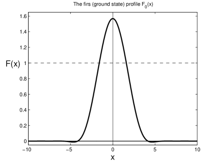
Figure 2. The first, ground state solution of the ODE (4.3).

In Figure 3, we show the second dipole-like profiles, where $F_{1}(x)$ denoted by the boldface line is the basic one corresponding to the L–S critical value. In addition, there exists a countable (this is not proved still) family of dipoles $\{F_{1}^{(k)}\}$, which differ by the structure of the internal zero close to the origin (in general, $k$ stands for the number of transversal zeros there, but this is not enough to uniquely identifying the pattern). By the dotted line, we denote another profile from the next family $\{F_{2}^{(k)}\}$; see below.

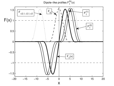
Figure 3. Some of the dipole-like solutions $F_{1}^{(k)}(x)$, $k=0,1,2$ of the ODE (4.3).

Figure 4 continues explaining further basic L–S patterns, where we show $F_{0}$, $F_{1}$, $F_{2}$, and $F_{3}$ (the dotted line). It is clearly seen that each $F_{k}$ has precisely $k$ “dominant” transversal zeros inside the support, which well corresponds to Sturm-like principle (not applicable here in the rigorous sense, since all the solutions are oscillatory and have infinitely many sign changes near interfaces).

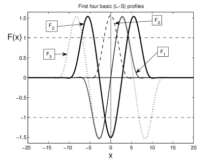
Figure 4. Four basic L–S patterns of the ODE (4.3).

In Figure 5, non L-S profiles from the family $\{F_{+2k}\}$ are presented. Figure 6 shows some profiles from the family $\{F_{+2,2k,+2}(x)\}$, which are also not expected to correspond to any L–S category/critical value.

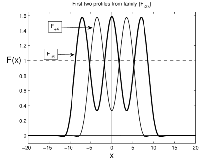
Figure 5. Solutions $F_{+4}(x)$ and $F_{+6}(s)$ of the ODE (4.3).

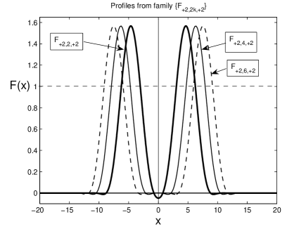
Figure 6. Solutions $\{F_{+2,2k,+2}(x)\}$ of the ODE (4.3).

First profiles from the family $\{F_{+2,2,...,2,+2}(x)\}$ (also non L–S) are shown in Figure 7.

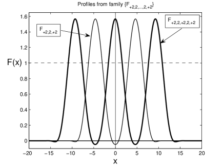
Figure 7. Solutions $\{F_{+2,2,...,2,+2}(x)\}$ of the ODE (4.3).

Finally, following [26]and using the above rather simple families of patterns, we claim that a pattern (possibly, a class of patterns) with an arbitrary multiindex of any length

(4.17) $$\sigma=\{\pm\sigma_{1},\sigma_{2},\pm\sigma_{3},\sigma_{4},...,\pm\sigma_{l}\}$$

can be constructed. Here, as above, each $\pm\sigma_{k}$ stands for the total number of successive intersections with the current equilibrium $\pm 1$, while $\sigma_{k}$ counts that with the trivial equilibrium $0$. E.g., in Figure 8, we show a single complicated profile $F_{\sigma}(x)$ with the index

(4.18) $$\sigma=\{+4,1,-4,1,+2,2,+4,1,-4,1,+8\}.$$

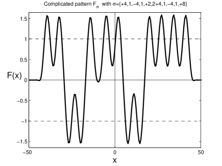
Figure 8. Solution $F_{+4,1,-4,1,+2,2,+4,1,-4,1,+8}(x)$ of the ODE (4.3).

Actually, the multiindex (4.17) can be rather arbitrary (with some natural restrictions on even local intersection numbers) and then takes finite parts of any admissible non-periodic fraction. Overall, this means chaotic features of the whole family of solutions $\{F_{\sigma}\}$. These chaotic types of behaviour are known for other fourth-order ODEs with coercive smooth operators, [45, p. 198].

5. No log-log for the TFE–4 with source

For the TFE–4 (1.27), the similarity substitution as in (4.1) yields another ODE:

(5.1) $$\textstyle{\frac{1}{2}\,\theta=-(\theta^{2}\theta^{\prime\prime\prime})^{\prime}+\theta^{3}\quad\mbox{in}\quad\mathbb{R}.}$$

To get equilibria $\pm 1$, we perform the change:

(5.2) $$\textstyle{\theta(x)=\frac{1}{\sqrt{2}}\,F(x)\quad\Longrightarrow\quad(F^{2}F^{\prime\prime\prime})^{\prime}=F^{3}-F\quad\mbox{in}\quad\mathbb{R}.}$$

Unlike the one in (4.1) and (4.3), the ODE in (5.2) does not admit a variational formulation. Nevertheless, there exist rather standard shooting arguments for detecting necessary similarity blow-up profiles; see references in [17, § 3]. In particular, the following asymptotic behaviour is known close to finite interfaces

(5.3) $$\textstyle{F(x)=\frac{1}{2}\,(x_{0}-x)_{+}^{2}\big{[}\sqrt{|\ln(x_{0}-x)|}+C+...\big{]}\quad\mbox{as}\quad x\to x_{0},}$$

where $C\in\mathbb{R}$ is an arbitrary constant. Overall, the asymptotic bundle (5.3) comprises two parameters $\{x_{0},C\}$, which are expected to be sufficient to shoot also two conditions at the origin:

(5.4) $$F^{\prime}(0)=F^{\prime\prime\prime}(0)=0\,\,\,(\mbox{symmetry})\quad\mbox{or}\quad F(0)=F^{\prime\prime}(0)=0\,\,\,(\mbox{anti-symmetry}).$$

Figure 9 shows the first nonnegative even profile $F_{0}(x)$ for $x>0$ with the symmetry conditions in (5.4) and the interface $x_{0}=2.83...\,.$ Hence, the answer to (1.3) is log-log $\not\exists$.

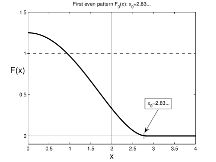
Figure 9. The first basic nonnegative solution $F_{0}(x)$ of the ODE in (5.2).

6. Quasilinear wave and nonlinear dispersion equations

6.1. The QWE–4

For (1.28), the similarity separable solution (2.1) is slightly different, but the ODE remains the same:

(6.1) $$\textstyle{u_{\rm S}(x,t)=\frac{1}{T-t}\,\theta(x),\quad\mbox{where}\quad 2\theta=\theta^{2}(-\theta^{(4)}+\theta).}$$

Hence, Proposition 2.1 holds, so we need the log-TWs for matching:

(6.2) $$\textstyle{u_{\rm log}(x,t)=\frac{1}{T-t}\,g(\eta),\,\,\eta=x+\lambda\ln(T-t)\,\Longrightarrow\,2g-3\lambda g^{\prime}+\lambda^{2}g^{\prime\prime}=g^{2}(-g^{(4)}+g).}$$

However, the necessary asymptotics is guaranteed by keeping just two terms:

(6.3) $$2g=-g^{2}g^{(4)}+...\,,$$

so that the only correction to (2.17) is the multiplier $\sqrt{2}$. The rest of the analysis remains the same as at the end of Section 2.

For the divergent wave model

(6.4) $$u_{tt}=-(u^{3})_{xxxx}+u^{3}$$

the log-log factor is nonexistent, since it admits separable compactly supported solutions

(6.5) $$\textstyle{u_{\rm S}(x,t)=\frac{1}{T-t}\,\theta(x)\quad\Longrightarrow\quad 2\theta=-(\theta^{3})^{(4)}+\theta^{3},}$$

which on scaling reduces to that in (4.1).

6.2. The NDE–4: non-divergent model

For (1.29), the similarity separable solution (2.1) is slightly different, but the ODE remains the same:

(6.6) $$\textstyle{u_{\rm S}(x,t)=(T-t)^{-\frac{1}{3}}\,\theta(x),\quad\mbox{where}\quad\frac{1}{3}\,\theta=\theta^{3}(\theta^{\prime\prime\prime}+\theta).}$$

Instead of (2.4), the nonexistence conclusion is governed by the following “local monotonicity” identity:

(6.7) $$\textstyle{-\frac{1}{3}\,\frac{1}{\theta}=\theta^{\prime}\theta^{\prime\prime}-\int(\theta^{\prime\prime})^{2}+\frac{1}{2}\,\theta^{2},}$$

so that sufficiently smooth solutions with $\theta=0$ at $\pm L$ (and $\theta\in H^{2}$) do not exist.

As the analogy to (2.12), consider the stationary equation:

(6.8) $$f(x):\quad f^{\prime\prime\prime}+f=0\quad\mbox{on}\quad(-L_{0},L_{0}),\quad f(-L_{0})=f^{\prime}(-L_{0})=0,\quad f(L_{0})=0,$$

where the zero at $x=L_{0}$ is assumed to be transversal with the behaviour (cf. the smoother one (2.18))

(6.9) $$f(x)=C_{1}(x-L_{0})(1+o(1))\quad\mbox{as}\quad x\to L_{0}^{-}\quad(C_{1}>0).$$

According to the problem (6.8), to avoid extra difficulties with rather obscure consequences, we consider (1.29) in $(-L_{0},L)\times(0,T)$, with $L>L_{0}$ (possibly, $L\gg L_{0}$ to avoid existence of other stationary profiles) and the same boundary conditions at the left-hand end point,

(6.10) $$u=u_{x}=0\quad\mbox{at}\quad x=-L_{0}\quad\mbox{and}\quad u=0\quad\mbox{at}\quad x=L.$$

Therefore, the log-log perturbation will penetrate into Inner Region-I from the right-hand singular point $x=L_{0}$, where the stationary solution (6.8) vanishes thus creating an internal singular layer to be resolved by using slowly moving log-TWs.

Thus, the log-TW ansatz yields the ODE

(6.11) $$\textstyle{u_{\rm log}(x,t)=(T-t)^{-\frac{1}{3}}g(\eta),\,\,\eta=x+\lambda\ln(T-t)\Longrightarrow\frac{1}{3}\,g-\lambda g^{\prime}=g^{3}(g^{\prime\prime\prime}+g).}$$

Close to the necessary point $x=L_{0}$, we keep as usual two terms that yields the desired behaviour:

(6.12) $$\textstyle{\frac{1}{3}\,g=g^{3}g^{\prime\prime\prime}+...\quad\Longrightarrow\quad g(\eta)\sim(-\eta)[\ln(-\eta)]^{\frac{1}{3}}\quad\mbox{as}\quad\eta\to-\infty.}$$

Similar to (2.21)–(2.22), matching the linear structure $(-\eta)$ in (6.12) with the linear one $\sim(L_{0}-x)$ in (6.9) yields

(6.13) $$A(t)\sim\big{[}\ln|\ln(T-t)|\big{]}^{\frac{1}{3}}(1+o(1))\quad\mbox{as}\quad t\to T^{-}.$$

Observe changing $\sqrt{(\cdot)}$ into the cubic root due to cubic nonlinearity $u^{3}$ in (1.29) instead of $u^{2}$ in other models. The choice of the quartic equation (1.29) was in fact generated by the possibility of such a transversal matching of “linear” structures. Some aspects of such a matching are still unclear and deserve further study.

6.3. No double-log in a divergent NDE

For the corresponding divergent NDE,

(6.14) $$u_{t}=(u^{4})_{xxx}+u^{4},$$

answering (1.3), one can construct separable blow-up solutions

(6.15) $$\textstyle{u_{\rm S}(x,t)=(T-t)^{-\frac{1}{3}}\,\theta(x)\quad\Longrightarrow\quad\frac{1}{3}\,\theta=(\theta^{4})^{\prime\prime\prime}+\theta^{4}.}$$

Looking for nonnegative solutions $\theta\geq 0$, on rescaling, yields

(6.16) $$\theta=3^{-\frac{3}{4}}F\quad\Longrightarrow\quad F^{\prime\prime\prime}+F-F^{\frac{1}{4}}=0\quad\mbox{in}\quad(-L_{0},L_{0}).$$

Unlike the ODE (4.3), this one admits solutions with a single interface (free-boundary) point $x=-L_{0}$ with the behaviour

(6.17) $$F(x)=(24)^{-\frac{4}{3}}(L_{0}+x)_{+}^{4}(1+o(1))\quad\mbox{as}\quad x\to-L_{0}^{+}.$$

In other words, we can set $F(x)\equiv 0$ for all $x<-L_{0}$. Therefore, moving such a profile $F(x)$, one can always satisfy the boundary condition at $x=L$ in (6.8) for any $L>0$. Typical solutions of the ODE (6.16) are shown in Figure 10, where positive humps can serve as blow-up patterns. Note that all such solutions are not oscillatory near finite interfaces, unlike those for the TFEs [17], where another third-order oscillatory ODE occurs. Thus, the similarity law (6.15) describes blow-up in the divergent model (6.14).

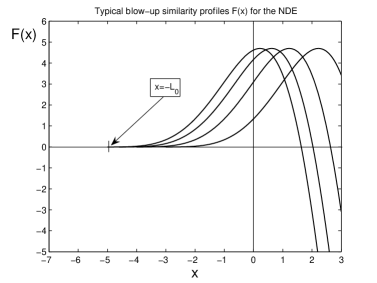
Figure 10. Blow-up patterns $F(x)$ satisfying (6.16) with the behaviour (6.17).

7. Final conclusion: blow-up log-log is universal in PDE theory

The above study allows us to fix the following conclusion: rather surprisingly,

(7.1) the factor $$\sqrt{\ln|\ln(T-t)|}$$ has a clear universality in blow-up

for different classes of higher-order (non-divergent) nonlinear evolution PDEs. The $\ln\,\ln$-factor also occurs in boundary regularity (Petrovskii-type) analysis for equations [25]

$$u_{t}=-u_{xxxx},\quad u_{t}=u_{xxx},\quad u_{t}=-(u^{3})_{xxxx},\quad\mbox{etc.}$$

It would be important, on the basis on the above discussion of various linear and nonlinear PDEs and by adding new asymptotic phenomena of necessity, to explain, in a more unified way, and to derive, formally or more justified, such a common matched asymptotic $\sqrt{\log\,\log}$-criterion.

References

- [1] U. Abresch and J. Langer, The normalized curve shortening flow and homothetic solutions, J. Differ. Geom., 23 (1986), 175–196.
- [2] S. Ahmanov, A. Sukhorukov, and R. Khokhlov, Self-focusing and self-trapping of intense light beams in a nonlinear medium, J. Exper. Theoret. Physics, 23 (1966), 1025–1033.
- [3] S. Angenent, On the formation of singularities in the curve shortening flow, J. Differ. Geom., 33 (1991), 601–633.
- [4] S. Angenent and J.J.L. Velázquez, Asymptotic shape of cusp singularities in curve shortening, Duke Math. J., 77 (1995), 71–110.
- [5] J. Angulo, J.L. Bona, F. Linares, and M. Scialom, Scaling, stability and singularities for nonlinear, dispersive wave equations: the critical case, Nonlinearity, 15 (2002), 759–786.
- [6] M. Berger, Nonlinearity and Functional Analysis, Acad. Press, New York, 1977.
- [7] F. Bernis and A. Friedman, Higher order nonlinear degenerate parabolic equations, J. Differ. Equat., 83 (1990), 179–206.
- [8] F. Bernis and J.B. McLeod, Similarity solutions of a higher order nonlinear diffusion equation, Nonl. Anal., 17 (1991), 1039–1068.
- [9] A. Brandenburg and E.G. Zweibel, The formation of sharp structures by ambipolar diffusion, Astrophys. J., 427 (1994), L91–L94.
- [10] C.J. Budd, Asymptotics of multibump blow-up self-similar solutions of the nonlinear Schrödinger equation, SIAM J. Appl. Math., 62 (2001), 801–830.
- [11] R.Y. Chiao, E. Garmire, and C.H. Townes, Self-trapping of optical beams, Phys. Rev. Lett., Nonl. Anal., 13 (1964), 479–482.
- [12] C.V. Coffman, Uniqueness of the ground state for and a variational characterization of other solutions, Arch. Rat. Mech. Anal., 46 (1972), 81–95.
- [13] R. Courant and D. Hilbert, Methods of Mathematical Physics, Vol. II, R. Courant, Partial Differential Equations, Intersci. Publ., J. Wiley & Sons, New York/London, 1962.
- [14] K. Deimling, Nonlinear Functional Analysis, Springer-Verlag, Berlin/Tokyo, 1985.
- [15] Yu.V. Egorov, V.A. Galaktionov, V.A. Kondratiev, and S.I. Pohozaev, Global solutions of higher-order semilinear parabolic equations in the supercritical range, Adv. Differ. Equat., 9 (2004), 1009–1038.
- [16] S.D. Eidelman, Parabolic Systems, North-Holland Publ. Comp., Amsterdam/London, 1969.
- [17] J.D. Evans, V.A. Galaktionov, and J.R. King, Source-type solutions of the fourth-order unstable thin film equation, Euro J. Appl. Math., 18 (2007), 273–321.
- [18] G. Fibich, F. Merle, and P. Raphael, Proof of a spectral property related to the singularity formation for the critical nonlinear Schrödinger equation, Physica D, 220 (2006), 1–13.
- [19] G. Fibich, N. Gavish, and X.-P. Wang, Singular ring solutions of critical and supercritical nonlinear Schrödinger equations, Physica D, 231 (2007), 55–86.
- [20] G.M. Fraĭman, Asymptotic stability of manifold of self-similar solutions in self-focusing, Zh. Èksper. Teoret. Fiz., 88 (1985), 390–400; Soviet Phys. JETP, 61 (1985), 228–233.
- [21] A. Friedman, Partial Differential Equations, Robert E. Krieger Publ. Comp., Malabar, 1983.
- [22] A. Friedman and B. McLeod, Blow-up of solutions of nonlinear degenerate parabolic equations, Arch. Rat. Mech. Anal., 96 (1986), 55–80.
- [23] V.A. Galaktionov, Shock waves and compactons for fifth-order nonlinear dispersion equations, Europ. J. Appl. Math., submitted.
- [24] V.A. Galaktionov, Formation of shocks and fundamental solution of a fourth-order quasilinear Boussinesq-type equation, Nonlinearity, to appear.
- [25] V.A. Galaktionov, On regularity of a boundary point in higher-order parabolic equations: a blow-up approach, NoDEA, submitted; ArXiv:0901.3986v1 [math.AP] 26 Jan 2009.
- [26] V.A. Galaktionov, E. Mitidieri, and S.I. Pohozaev, Variational approach to complicated similarity solutions of higher-order nonlinear evolution equations of parabolic, hyperbolic, and nonlinear dispersion types, In: Sobolev Spaces in Mathematics. II, Appl. Anal. and Part. Differ. Equat., Series: Int. Math. Ser., Vol. 9, V. Maz’ya Ed., Springer, 2009.
- [27] V.A. Galaktionov and S.R. Svirshchevskii, Exact Solutions and Invariant Subspaces of Nonlinear Partial Differential Equations in Mechanics and Physics, ChapmanHall/CRC, Boca Raton, Florida, 2007.
- [28] V.A. Galaktionov and J.L. Vazquez, A Stability Technique for Evolution Partial Differential Equations. A Dynamical Systems Approach, Progr. in Nonl. Differ. Equat. and Their Appl., Vol. 56, Birkhäuser, Boston/Berlin, 2004.
- [29] A.D. Ionescu and C.E. Kenig, Carleman inequalities and uniqueness of solutions of nonlinear Schrödinger equations, Acta. Math., 193 (2004), 193–239.
- [30] P. Kelley, Self-focusing of optical beams, Phys. Rev. Lett., Nonl. Anal., 15 (1965), 1005–1008.
- [31] O.D. Kellogg, Foundations of Potential Theory, Fred. Ungar Publ. Comp., New York, 1929.
- [32] C.E. Kenig and F. Merle, Global well-posedness, scattering and blow-up for the energy-critical, focusing, non-linear Schrödinger equation in the radial case, Invent. math., 166 (2006), 645–675.
- [33] N.E. Kosmatov, V.F. Shvets, and V.E. Zakharov, Computer simulation of wave collapses in the nonlinear Schrödinger equation, Phys. D, 52 (1991), 16–35.
- [34] M.A. Krasnosel’skii and P.P. Zabreiko, Geometrical Methods of Nonlinear Analysis, Springer-Verlag, Berlin/Tokyo, 1984.
- [35] M.J. Landman, G.C. Papanicolau, C. Sulem, and P.-L. Sulem, Rate of blow-up for solutions of the nonlinear Schrödinger equation at critical dimension, Phys. Rev. A(3), 38 (1988), 3837–3843.
- [36] X. Li and J. Zhang, Rate of -concentration of blow-up solutions for critical nonlinear Schrödinger equation, Proc. Amer. Math. Soc., 135 (2007), 3253–3262.
- [37] B.C. Lou, Resistive diffusion of force-free magnetic fields in a passive medium, Astrophys. J., 181 (1973), 209–226; 184 (1973), 917–929.
- [38] M.A. Naimark, Linear Differential Operators, Part 1, Frederick Ungar Publ. Co., New York, 1967.
- [39] F. Merle and P. Raphael, On universality of blow-up profile for critical nonlinear Schrödinger equation, Invent. math., 156 (2004), 565–672.
- [40] F. Merle and P. Raphael, On a sharp lower bound on the blow-up rate for the critical nonlinear Schrödinger equation, J. Amer. Math. Soc., 19 (2005), 37–90.
- [41] F. Merle and P. Raphael, The blow-up dynamics and upper bound on the blow-up rate for critical nonlinear Schrödinger equation, Ann. Math., 161 (2005), 157–222.
- [42] F. Merle and P. Raphael, Profiles and quantization of the blow-up mass for critical nonlinear Schrödinger equation, Comm. Math. Phys., 253 (2005), 675–704.
- [43] B.J. LeMesurier, G.C. Papanicolau, C. Sulem, and P.-L. Sulem, Local structure of the self-focusing singularity of the nonlinear Schrödinger, Phys. D, 32 (1988), 210–226.
- [44] L.V. Ovsiannikov, Group properties of a nonlinear heat equation, Dokl. Akad. Nauk SSSR, 125 (1959), 492–495.
- [45] L.A. Peletier and W.C. Troy, Spatial Patterns: Higher Order Models in Physics and Mechanics, Birkhäuser, Boston/Berlin, 2001.
- [46] G. Perelman, On the formation of singularities in solutions of the critical nonlinear Schrödinger equation, Ann. Henri Poincaré, 2 (2001), 605–673.
- [47] J. Petrowsky, Über die Lösungen der ersten Randwertaufgabe der Wärmeleitungsgleichung, Uenye Zapiski Moscovsk. Gosud. Univ., No. 2 (1934), 55–59, Moscow, USSR (in German, with Russian summary).
- [48] I.G. Petrovsky, Zur ersten Randwertaufgabe der Wärmeleitungsleichung, Compositio Math., 1 (1935), 383–419.
- [49] F. Planchon and P. Raphaël, Existence and stability of the log–log blow-up dynamics for the -critical nonlinear Schrödinger equation in a domain, Ann. Henri Poincaré, 8 (2007), 1177–1219.
- [50] S.I. Pohozaev, On an approach to nonlinear equations, Soviet Math. Dokl., 20 (1979), 912-916.
- [51] S.I. Pohozaev, The fibering method in nonlinear variational problems, Pitman Research Notes in Math., Vol. 365, Pitman, 1997, pp. 35-88.
- [52] P. Raphaël, Existence and stability of a solution blowing up on a sphere for an supercritical nonlinear Schrödinger equation, Duke Math. J., 134 (2006), 199–258.
- [53] A.A. Samarskii, V.A. Galaktionov, S.P. Kurdyumov, and A.P. Mikhailov, Blow-up in Quasilinear Parabolic Equations, Walter de Gruyter, Berlin/New York, 1995.
- [54] A.A. Samarskii, N.V. Zmitrenko, S.P. Kurdyumov, and A.P. Mikhailov, Thermal structures and fundamental length in a medium with non-linear heat conduction and volumetric heat sources, Soviet Phys. Dokl., 21 (1976), 141–143.
- [55] A.I. Smirnov and G.M. Fraĭman, The interaction representation in the self-focusing theory. Wave collapses (Novosibirsk,1988), Physica D, 52 (1991), 2–15.
- [56] R.S. Steinolfson and T. Tajima, Energy building in coronal magnetic flux tubes, Astrophys. J., 322 (1987), 503–511.
- [57] C. Sulem and P.-L. Sulem, The Nonlinear Schrödinger Equation, Springer-Verlag, New York, 1999.
- [58] S.I. Vainshtein, Z. Mikić, and R. Sagdeev, Compression of the current sheet and its impact into the reconnection rate, arXiv:0711.1666v3 [astro-ph] 14 Nov 2007.
- [59] S.N. Vlasov, L.V. Piskunova, and V.I. Talanov, Structure of the field near a singularity arising from self-focusing in a cubically nonlinear medium, Sov. Phys. JETP, 48 (1978), 808–812.
- [60] P.A. Watterson, Force-Free Magnetic Evolution in the Reversed-Field Pinch, Thesis, Cambridge Univ., Cambridge, 1985.
- [61] P.A. Watterson, Infinite contraction in force-free magnetic field evolution in cylindrical geometry, J. Plasma Phys., 35 (1986), 273–293.
- [62] N. Wiener, The Dirichlet problem, J. Math. and Phys. Mass. Inst. Tech., 3 (1924), 127–146; reprinted in: N. Wiener, Collected Works with Commentaries, Vol. I, ed. P. Masani, Mathematicians of Our Time 10, MIT Press, Cambridge, Mass., 1976, pp. 394–413.
- [63] V.E. Zakharov, Private communication with the author, Bristol, October 1991.