Universal scaling in nonequilibrium transport through an Anderson impurity

Abstract

Using non-equilibrium renormalized perturbation theory, we calculate the conductance $G$ as a function of temperature $T$ and bias voltage $V$ for an Anderson model, suitable for describing transport properties through a quantum dot. For renormalized parameters that correspond to the extreme Kondo limit, we do not find a simple scaling formula beyond a quadratic dependence in $T$ and $V$. However, if valence fluctuations are allowed, we find excellent agreement with recent experiments.

Universality is one of the most beautiful and useful concepts in physics. In general, the physical properties of a system depend on a certain number of parameters which change for different experimental realizations. However, in favorable cases, physical observables are described by the same universal function, once the different physical magnitudes are scaled appropriately. For example in the case of the temperature dependence of the conductance through one quantum dot $G(T)$ in the limit of zero bias voltage $V$, once a characteristic energy scale $T_{K}$ (the Kondo temperature) is identified, the conductance of different systems is very well described by the same universal function $G(T/T_{K})$, even if the systems have very different $T_{K}$.gold ; grobis Scaling and universality are concepts which are quite naturally connected to renormalization group treatments of the Anderson model in the Kondo regime (Coulomb repulsion $U$ much larger than the resonant level width $\Delta$), and in fact numerical renormalization group (NRG) calculations reproduce the scaling mentioned above and in other physical properties.bulla ; chz

Theoretically, the situation is much more difficult in the nonequilibrium situation which arises for a finite bias voltage between the leads connected to the quantum dot in the experiment. Only recently, extensions to the nonequilibrium case of essentially exact techniques such as NRG anders and exact Bethe ansatz mehta were proposed, while approximations used at equilibrium have shortcomings when extended to the nonequilibrium case. none Nevertheless, using a Fermi liquid approach, based on perturbation theory (PT) in $U/\Delta$, and Ward identities, Oguri has determined exactly the scaling for $T$ and $eV$ small compared to $T_{K}$ for the Anderson model ogu

$$G(T,V)=G_{0}\left[1-c_{T}\left(\frac{T}{T_{K}}\right)^{2}-\alpha\,c_{T}\left(\frac{eV}{kT_{K}}\right)^{2}+\dots\right],$$ (1)

where $G_{0}=G(0,0)$ and the values of $c_{T}$ and $\alpha$ are discussed below.

Recent experiments in GaAs quantum dots for different situations in the nonequilibrium regime,grobis for low $T$ and $V$ have found that $G(T,V)$ is well described by a universal scaling function that extends Eq. (1) to higher temperatures

$$\frac{G(T,V)}{G_{E}(T)}\simeq 1-\frac{\alpha\,c_{T}(eV/kT_{K})^{2}}{1+(\gamma/\alpha-1)\,c_{T}\,(T/T_{K})^{2}}.$$ (2)

Here $c_{T}\simeq 5.488$ is fixed by Eqs. (1) and (3), $\alpha=0.10\pm 0.015$, $\gamma=0.5\pm 0.1$ and $G_{E}(T)$ is an empirical curve obtained from a fit to NRG results:

$$G_{E}(T)=\frac{G_{0}}{\left[1+(2^{1/s}-1)(T/T_{K})^{2}\right]^{s}},$$ (3)

with $s=0.21$ for an impurity with total spin $S=1/2$. From these equations, one can see that $\alpha$ is the ratio of the term of order $[eV/(kT_{K})]^{2}$ with respect to that of order $\left(T/T_{K}\right)^{2}$ in the decrease in the conductance, while $\gamma$ represents the effect of terms $[eV/(kT_{K})]^{2}\left(T/T_{K}\right)^{2n}$ with integer $n>1$.

From an exactly solvable anisotropic Kondo model,schi one extracts $\alpha=3/\pi^{2}\simeq 0.30$ and $\gamma=2(\pi T_{K}/T_{a})^{2}/c_{T}\simeq 3.60(T_{K}/T_{a})^{2}$, where $T_{a}$ is an energy scale of the order of $T_{K}$. To our knowledge, no other precise information on $\gamma$ exists.

The purpose of this work is to test the observed scaling relation and calculate $\gamma$ in the impurity Anderson model, using renormalized PT (RPT).he1 The basic idea of RPT is to reorganize the PT in terms of fully dressed quasiparticles in a Fermi liquid picture. The main advantage is that even in the strong coupling (SC) limit $U\rightarrow\infty$, for which ordinary PT in $u=U/(\pi\Delta)$ becomes invalid, the corresponding ratio between renormalized parameters (denoted by a tilde) becomes $\widetilde{u}\equiv\widetilde{U}/(\pi\widetilde{\Delta})\rightarrow 1$, being $\widetilde{u}<1$ for finite $U$.he1 For nontrivial cases, already free quasiparticles (taking $\widetilde{U}=0$, which is similar to slave bosons in a mean field approximation vaug ) reproduce very well the low-frequency part of the equilibrium spectral density at the quantum dot. An example is a case in which the Kondo peak is split in two.vaug $\widetilde{U}$ (proportional to the full vertex) represents the “residual” interaction between quasiparticles. Calculating the renormalized retarded self-energy $\widetilde{\Sigma}^{r}$ within nonequilibrium RPT up to second order in $\widetilde{u}$, $T$ and $V$ leads to the exact result Eq. (1).ogu ; hbo Here we calculate numerically $\widetilde{\Sigma}^{r}$ up to order $\widetilde{u}^{2}$, for finite $kT$ and $eV$ but smaller or of the order of the Kondo energy $kT_{K}$.

Ordinary PT up to second order in $U$ supplemented by an interpolative perturbative approach (IPA), levy ; kaju (which corrects the second-order result in order to reproduce exactly the atomic limit $U/\Delta\rightarrow+\infty$) has been shown to describe well the conductance through a quantum dot for $U\leq 8\Delta$.pro The results agree with those obtained using the finite temperature density matrix renormalization group method.maru Comparison of the spin dependent IPA pc ; lady with exact diagonalization in finite systems shows very good agreement for $U=6.25\Delta$.pc The extension of PT in $U^{2}$ to the nonequilibrium case has been considered by Hershfield et al.hersh They found that for finite $V$, the current is conserved only in the electron-hole symmetric Anderson model (SAM). Different self-consistent approaches were proposed to overcome this shortcoming, by a suitable election of the unperturbed Hamiltonian.none ; levy While these approaches work well in absence of a magnetic field $B$, numerical difficulties persist for small non-vanishing $B$ and $V$.none Here we will take $B=0$ and parameters corresponding to the SAM for our numerical integrations. In this case the current is conserved for each spin without the need to solve self-consistent equations.none

We use the spin 1/2 Anderson model to describe a quantum dot interacting with two conducting leads, one at the left and one at the right, with chemical potentials $\mu_{L}$ and $\mu_{R}$ respectively, with $\mu_{L}-\mu_{R}=eV$. We define the zero of energy by $\mu_{L}=eV\Delta_{R}/\Delta$, where $\Delta=\Delta_{L}+\Delta_{R}$ and $\Delta_{\nu}=\pi\sum_{k}|V_{k\nu}|^{2}\delta(\omega-\varepsilon_{eff}^{\sigma})$ (neglecting here the small none dependence on $\omega$). The Hamiltonian is split into a noninteracting part $H_{0}$ and a perturbation $H^{\prime}$ as

$$\left.\begin{aligned} H&=H_{0}+H^{\prime},\\ H_{0}&=\sum_{k\nu\sigma}\varepsilon_{k\nu}\,c_{k\nu\sigma}^{\dagger}c_{k\nu\sigma}+\sum_{\sigma}\varepsilon_{eff}^{\sigma}\,n_{d\sigma}\\ &+\sum_{k\nu\sigma}\left(V_{k\nu}\,c^{\dagger}_{k\nu\sigma}d_{\sigma}+\text{H.c.}\right),\\ H^{\prime}&=\sum_{\sigma}\left(E_{d}-\varepsilon_{eff}^{\sigma}\right)\,n_{d\sigma}+U\,n_{d\uparrow}n_{d\downarrow},\end{aligned}\right.$$ (4)

where $\nu=L,R$ refers to the left and right leads. In general $\varepsilon_{eff}^{\sigma}$ should be determined selfconsistently, but for the SAM with $B=0$, $\varepsilon_{eff}^{\sigma}=0$.none We obtain the conductance $G=dI/dV$ from numerical differentiation of the current $I$, which can be written as meir

$$I=\frac{2e}{h}\int d\omega A\pi\Delta\rho(\omega)[f_{L}(\omega)-f_{R}(\omega)],$$ (5)

where $f_{\nu}(\omega)=f(\omega-\mu_{\nu})$, $f(\omega)=1/(e^{\omega/kT}+1)$, $A=4\Delta_{L}\Delta_{R}/\Delta^{2}$ indicates the degree of asymmetry of the hybridization of the dot with both leads, and $\rho(\omega)=-\text{Im}G_{d\sigma}^{r}(\omega)/\pi$ where $G_{d\sigma}^{r}(\omega)$ is the retarded Green’s function of the electrons at the dot for spin $\sigma$, which can be written as none

$$G_{d\sigma}^{r}(\omega)=\frac{1}{\omega-\varepsilon_{eff}^{\sigma}+i\Delta-\Sigma_{\sigma}^{r}(\omega)}.$$ (6)

Within RPT, the low frequency part of $G_{d\sigma}^{r}(\omega)$ can be approximated as he1

$$\widetilde{G}_{d\sigma}^{r}(\omega)\simeq\frac{z}{\omega-\widetilde{\varepsilon}_{eff}^{\sigma}+i\widetilde{\Delta}-\widetilde{\Sigma}_{\sigma}^{\text{rem}}(\omega)},$$ (7)

where $z=[1-\partial\Sigma_{\sigma}^{r}/\partial\omega]^{-1}$, $\widetilde{\varepsilon}_{eff}^{\sigma}=z[\varepsilon_{eff}^{\sigma}+\Sigma_{\sigma}^{r}(0)]$, $\widetilde{\Delta}=z\Delta$, and $\widetilde{\Sigma}_{\sigma}^{\text{rem}}(\omega)=z\Sigma_{\sigma}^{\text{rem}}(\omega)$, where the remainder retarded self-energy is defined as

$$\Sigma_{\sigma}^{\text{rem}}(\omega)=\Sigma_{\sigma}^{r}(\omega)-\Sigma_{\sigma}^{r}(0)-\omega\partial\Sigma_{\sigma}^{r}/\partial\omega.$$ (8)

In Eqs. (7) and (8), $\Sigma_{\sigma}^{r}(0)$ and $\partial\Sigma_{\sigma}^{r}/\partial\omega$ are evaluated at $\omega=T=V=0$. A comparison between $G_{d\sigma}^{r}(\omega)$ (calculated within PT) and $\widetilde{G}_{d\sigma}^{r}(\omega)$ with $\widetilde{\Sigma}_{\sigma}^{r}(\omega)=0$, for a case with non-trivial frequency dependent $\Delta(\omega)$ is provided in Ref. vaug, , showing a very good agreement for low $|\omega|$. For large values of $U/\Delta$, ordinary PT in $U$ is not reliable and $z$ is in principle not known, although it can be obtained from exact Bethe ansatz calculations. However, replacing $\Delta$ by $\widetilde{\Delta}/z$ in Eq. (5), $z$ cancels and the current is expressed in terms of renormalized parameters $\widetilde{\varepsilon}_{eff}^{\sigma}$, $\widetilde{\Delta}$, and $\widetilde{\Sigma}_{\sigma}^{\text{rem}}(\omega)$. In the SC limit $U/\Delta\rightarrow\infty$, Hewson he1 has shown that the ratio of renormalized parameters is $\widetilde{u}=\widetilde{U}/(\pi\widetilde{\Delta})=1$ and furthermore, defining the Kondo temperature $T_{K}^{C}$ by the linear term in the specific heat in this limit $\gamma_{C}=\pi^{2}k/(6T_{K}^{C})$, one obtains $\widetilde{\Delta}=4kT_{K}^{C}/\pi$. In the SAM at $B=0$, which we shall use, $\Delta_{L}=\Delta_{R}$, $E_{d}=-U/2$, and this implies $\widetilde{\varepsilon}_{eff}^{\sigma}=0$.vaug Experimentally, $\Delta_{L}\sim\Delta_{R}$ and the scaling results do not depend on the gate voltage, which controls $E_{d}$. Furthermore, the value of $E_{d}$ is irrelevant in the SC limit. This justifies the use of the SAM. Finally we use

$$\widetilde{\Sigma}_{\sigma}^{\text{rem}}(\omega)=\widetilde{\Sigma}_{\sigma}^{r}(\omega)-\widetilde{\Sigma}_{\sigma}^{r}(0)-\omega\partial\widetilde{\Sigma}_{\sigma}^{r}/\partial\omega,$$ (9)

where $\widetilde{\Sigma}_{\sigma}^{r}(\omega)$ is obtained using nonequilibrium PT up to second order in $\widetilde{u}$ Details of the nonequilibrium RPT were published in previous works ogu ; hbo . The second-order diagram has two sums over Matsubara frequencies. For $\widetilde{\Delta}$ independent of frequency, one of the sums can be done analytically, which simplifies the numerical evaluation. Explicit expressions for the retarded and lesser self-energies are given in the appendix of Ref. none, . It is known yam that $\partial\widetilde{\Sigma}_{\sigma}^{r}/\partial\omega=-(3-\pi^{2}/4)\widetilde{u}^{2}$.

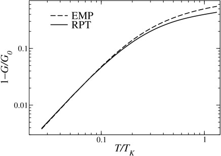
Figure 1: Conductance shift for $V=0$ as a function of temperature for $\widetilde{u}=1$. Dashed line corresponds to the empirical (EMP) curve Eq. (3).

We begin by analyzing the case $\widetilde{u}=1$, which corresponds to the strong coupling (SC) limit $U\rightarrow\infty$. As in the experiment, grobis we obtain $T_{K}$ by a fit of the temperature dependence of the conductance for $V=0$ to Eq. (3) for $T/T_{K}<0.25$. In Fig. 1 we compare Eq. (3) with our result. The fit is very good for low $T/T_{K}$, while for $T/T_{K}\simeq 1$, our result lies below the empirical curve. Remarkably, this is also the case of the experimental results.grobis This deviation however is outside the region of the fit and is irrelevant in the following discussion. From the fit we obtain $kT_{K}=0.757\widetilde{\Delta}$. The exact results to order $T^{2}$ and $V^{2}$ can be written in the form ogu

$$\frac{G}{G_{0}} \simeq 1-\frac{\pi^{2}(1+2\widetilde{u}^{2})}{3}\left(\frac{kT}{\widetilde{\Delta}}\right)^{2}$$ (10)

$$-\frac{4-3A+(2+3A)\widetilde{u}^{2}}{4}\left(\frac{eV}{\widetilde{\Delta}}\right)^{2}.$$

Note that in the Kondo limit $\widetilde{u}\rightarrow 1$, the coefficients are independent of the asymmetry parameter $A$, in agreement with recent calculations with the Kondo model.sela

A comparison with the expansion of Eq. (3) (for $V=0$) up to second order in $T$ leads to

$$\frac{kT_{K}}{\widetilde{\Delta}}=\frac{3s(2^{1/s}-1)}{\pi^{2}(1+2\widetilde{u}^{2})},$$ (11)

which for $\widetilde{u}=1$ implies $T_{K}=0.746\widetilde{\Delta}/k=0.949T_{K}^{C}$. The small discrepancy with the value $kT_{K}=0.757\widetilde{\Delta}$ obtained from the fit is due to the finite temperature interval used for fitting.

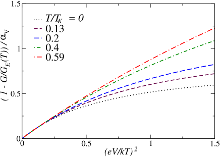
Figure 2: (Color online) Scaled conductance shift as a function of bias voltage for different temperatures and $\widetilde{u}=1$.

Next we calculate the conductance $G=dI/dV$ for finite $T$ and $V$, by numerical differentiation of Eq. (5) and compare the results with Eqs. (2) and (3). To obtain $\gamma$ we have fitted the current to a polynomial with odd powers of $V$ up to $V^{3}$within the range $0\leq eV/kT_{K}\leq 0.4$, as in the experiments. Inclusion of terms of order $V^{5}$ practically does not modify the results. The resulting shift in the conductance $(1-G/G_{E}(T))/{\alpha}_{V}$ scaled as in the experimental work with ${\alpha}_{V}=\alpha c_{T}/[1+(\gamma/\alpha-1)c_{T}(T/T_{K})^{2}],$ is shown in Fig. 2.

From the fit for $T=0$ we obtain $\alpha=0.151$. This agrees with Eq. (10), which predicts a ratio of the coefficients of the $V$ and $T$ dependence of the conductance [see Eq. (1)] $\alpha=3/(2\pi^{2})=0.152$ for $\widetilde{u}=1$, independently of the asymmetry $A$. . The small discrepancy is probably due to numerical errors in the integration near the singularities of the integrand.none The resulting values of $\gamma$ are near 0.75 for $0.13\leq T/T_{K}\leq 0.4$ and increase to 0.91 for $T/T_{K}=0.59$ and 1.2 for $T/T_{K}=0.79$ (not shown). These values are larger larger than the experimentally reported $\gamma=0.5\pm 0.1$. In addition, while the quadratic scaling with $V$ was expected, for most cases the observed exponent $\alpha=0.10\pm 0.015$ is smaller than the value $\alpha_{\text{SC}}^{\text{SAM}}=3/(2\pi^{2})$ of the SAM in the SC limit $U\rightarrow\infty$. Note however that for some of the measured systems $\alpha$ approaches this value (Fig. 3 of Ref. grobis, for $V_{G}\sim-0.195$ mV). In addition, in comparison with other theoretical predictions for $\alpha$, $3/\pi^{2}$ (Ref. schi, ), $3/(8\pi^{2})$ (Ref. kami, ), and $4/\pi^{2}$ (Ref. konik, ), the above value of $\alpha$ lies closer to experiment. However, it is clear that the Anderson model in the SC limit is not able to reproduce quantitatively the experiment.

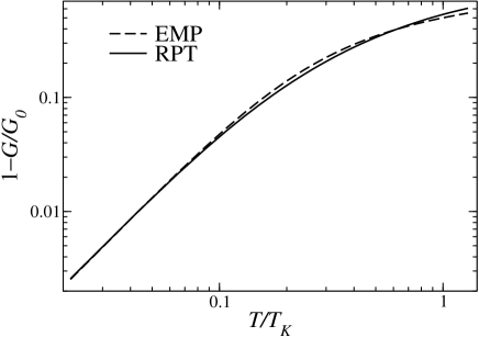
Figure 3: Conductance shift for $V=0$ as a function of temperature for $\widetilde{u}=0.365$. Dashed line corresponds to Eq. (3).

A value of $\alpha<\alpha_{\text{SC}}^{\text{SAM}}$ can be obtained decreasing $\widetilde{u}$ [see Eq. (10)] allowing some degree of intermediate valence. We explore this possibility, within the SAM, allowing finite $U$ and therefore $\widetilde{u}<1$. This means that while the average occupation of the dot is kept at the same value ($n=1$ in the SAM), some charge fluctuations with the neighboring configurations is allowed. From Eqs. (1) and (10) one sees that $\alpha=0.1$ implies $\widetilde{u}=0.365$. We have repeated the calculations for this value of $\widetilde{u}$. The conductance as a function of temperature is displayed in Fig. 3. We see that in this case, our result lies even closer to the phenomenological curve, indicating that the effect of temperature beyond $T^{2}$ is well described by our approximation (which assumed $\widetilde{u}$ independent of $T$ and $V$). Proceeding with the fit as in the experiment, we obtain $T_{K}=1.159\widetilde{\Delta}$, while Eq. (11) gives $T_{K}=1.147\widetilde{\Delta}/k=1.461T_{K}^{C}$.

In Fig. 4 we show the scaled shift in the conductance $(1-G/G_{E}(T))/{\alpha}_{V}$ [see Eq. (3)] for $\widetilde{u}=0.365$ as a function of the applied voltage for several temperatures.

The corresponding values of $\gamma$ are 0.75, 0.57, 0.49, 0.43 for $T/T_{K}$ =0.17, 0.35, 0.52, and 0.69 respectively. Thus except for the smallest temperatures $T/T_{K}\leq 0.17$, in this case $\gamma$ agrees with the experimental value $\gamma=0.5\pm 0.1$.

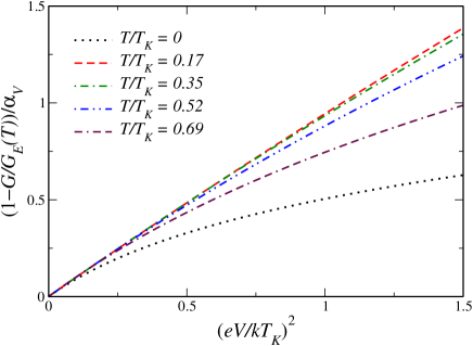
Figure 4: (Color online) Scaled conductance shift as a function of bias voltage for different temperatures and $\widetilde{u}=0.365$.

The reader might wonder if different physical situations in which the Kondo temperature can vary within a factor two are consistent with similar values of the renormalized ratio $\widetilde{u}=\widetilde{U}/(\pi\widetilde{\Delta})$. In fact, while the Kondo temperature decreases exponentially by increasing the ratio of the bare parameters $u=U/\pi\Delta$, $\widetilde{u}$ increases much slower,he1 ; ogu being of course $\widetilde{u}\sim u$ for small $u$ (including $u\sim 0.4$) and saturating at $\widetilde{u}=1$, for $u\rightarrow\infty$.

Finally, we note that if Eq. (1) with arbitrary exponents is used to fit the conductance with finite voltage and temperature ranges,grobis the resulting exponents are slightly below 2 in agreement with experiment.grobis

In summary, using nonequilibrium renormalized perturbation theory up to second order in the renormalized perturbation parameter $\widetilde{u}$ for the Anderson model in the symmetric case, we have examined the scaling behaviour of the conductance, including terms beyond those quadratic in temperature and bias voltage. In the strong coupling limit, the model predicts an effect of voltage which is 50% higher than observed and the effects of terms of order $(VT)^{2}$ disagree with experiment. If instead an important degree of valence fluctuations is allowed, we obtain good agreement with recent experimental results.

The authors are supported by CONICET. This work was done in the framework of projects PIP 5254 of CONICET and PICT 2006/483 of the ANPCyT.

References

- (1) D. Goldhaber-Gordon, J. Göres, M. A. Kastner, H. Shtrikman, D. Mahalu, and U. Meirav, Phys. Rev. Lett. 81, 5225 (1998).
- (2) M. Grobis, I. G. Rau, R. M. Potok, H. Shtrikman, and D. Goldhaber-Gordon, Phys. Rev. Lett. 100, 246601 (2008).
- (3) R. Bulla, T. A. Costi, and T. Pruschke, Rev. Mod. Phys.. 80, 395 (2008); references therein.
- (4) T. A. Costi, A. C. Hewson, and V. Zlatić, J. Phys. Condens. Matter 6, 2519 (1994).
- (5) F. B. Anders, Phys. Rev. Lett. 101, 066804 (2008).
- (6) P. Mehta and N. Andrei, Phys. Rev. Lett. 96, 216802 (2006).
- (7) A. A. Aligia, Phys. Rev. B 74, 155125 (2006).
- (8) A. Oguri, J. Phys. Soc. Jpn. 74, 110 (2005).
- (9) A. Schiller and S. Hershfield, Phys. Rev. B 51, 12896(R) (1995).
- (10) A. C. Hewson, Phys. Rev. Lett. 70, 4007 (1993).
- (11) A. C. Hewson, J. Bauer, and A. Oguri, J. Phys. Cond. Matt. 17, 5413 (2005).
- (12) L. Vaugier, A. A. Aligia, and A. M. Lobos, Phys. Rev. Lett. 99, 209701 (2007); Phys. Rev. B 76, 165112 (2007).
- (13) A. Levy-Yeyati, A. Martín-Rodero, and F. Flores, Phys. Rev. Lett. 71, 2991 (1993).
- (14) H. Kajueter and G. Kotliar, Phys. Rev. Lett. 77, 131 (1996).
- (15) A.A. Aligia and C.R. Proetto, Phys. Rev. B 65, 165305 (2002).
- (16) I. Maruyama, N. Shibata, and K. Ueda, J. Phys. Soc. Jpn. 73, 3239 (2004).
- (17) A.A. Aligia, Phys. Rev. B 66, 165303 (2002).
- (18) A. A. Aligia and L. A. Salguero, Phys. Rev. B 70, 075307 (2004); Phys. Rev. B 71, 169903(E) (2005).
- (19) S. Hershfield, J.H. Davies, and J.W. Wilkins, Phys. Rev. B 46, 7046 (1992).
- (20) Y. Meir and N. S. Wingreen, Phys. Rev. Lett. 68, 2512 (1992).
- (21) K. Yamada, Prog. Theor. Phys. 53, 970 (1975).
- (22) E. Sela, arXiv:0906.3729
- (23) A. Kaminski, Y. V. Nazarov, and L. I. Glazman, Phys. Rev. B 62, 8154 (2000).
- (24) R. M. Konik, H. Saleur, and A. Ludwig, Phys. Rev. B 66, 125304 (2002).