Microlensing towards the LMC revisited by adopting a non–Gaussian velocity distribution for the sources

Abstract

Aims. We discuss whether the Gaussian is a reasonable approximation of the velocity distribution of stellar systems that are not spherically distributed.

Methods. By using a non-Gaussian velocity distribution to describe the sources in the Large Magellanic Cloud (LMC), we reinvestigate the expected microlensing parameters of a lens population isotropically distributed either in the Milky Way halo or in the LMC (self lensing). We compare our estimates with the experimental results of the MACHO collaboration.

Results. An interesting result that emerges from our analysis is that, moving from the Gaussian to the non-Gaussian case, we do not observe any change in the form of the distribution curves describing the rate of microlensing events for lenses in the Galactic halo. The corresponding expected timescales and number of expected events also do not vary. Conversely, with respect to the self-lensing case, we observe a moderate increase in the rate and number of expected events. We conclude that the error in the estimate of the most likely value for the MACHO mass and the Galactic halo fraction in form of MACHOs, calculated with a Gaussian velocity distribution for the LMC sources, is not higher than $2\%$.

1 Introduction

Galaxies are complex, collisionless, gravitationally-bound systems formed by secular gravitational self-interaction and collapse of its constituents. Significant progress has been made in both observational and theoretical studies developed to improve our understanding of the evolutionary history of galaxies and the physical processes driving their evolution, leading to the Hubble sequence of galaxy type that we observe today. However, many aspects of their features, such as morphology, compositions, and kinematics, still remain unclear. In particular, it is not obvious how the velocities of their constituent (in particular stellar) components can be described, because we cannot consider them to be isotropically distributed at any point. Little is known about the velocity distribution (VD) of the stellar populations of galactic components. While the distribution of stellar velocities in an elliptical galaxy is generally reasonably close to a Gaussian, analyses of the line-of-sight (l.o.s.) velocity distributions of disk galaxies have shown that these distribution are highly non-Gaussian (Binney & Merrifield (1998)).

Today, one of the most important problems regarding the composition of the Milky Way (MW) concerns the existence of dark, compact agglomerates of baryons in the Galactic halo, the so-called MACHOs (MAssive Compact Halo Objects). From the experimental point of view, several observational groups have attempted to detect these objects by performing microlensing surveys in the directions of the Large Magellanic Cloud (LMC), Small Magellanic Cloud, and M31. Two groups (MACHO and POINT-AGAPE) reported similar conclusions, despite the fact that they observed different targets (LMC and M31), that is roughly $20\%$ of the halo mass must be in the form of MACHOs (Alcock et al. alcock00 (2000); Calchi Novati et al. (2005)). However, the interpretation of their data is controversial because of the insufficient number of events detected, and the existing degeneration among the parameters. Discordant results have been reported by other experimental teams (Tisserand et al. (2007); de Jong et al. (2004)).

Accurate theoretical estimates of the microlensing parameters, supported by statistical analysis, are fundamental to the interpretation of the experimental results. However, there are many uncertain assumptions in the adopted lens models. These uncertainties, that could lead towards an incorrect interpretation of the data, are mostly related to the shape of the individual galactic components and the kinematics of the lens population.

One of the first problems to be raised by the scientific community concerned the shape of the Galactic dark halo. Unfortunately, information that can be extracted from observations of high-velocity stars and satellite galaxies does not place strong constraints on its shape. In the absence of precise data, we are aided by computational models of the formation of galaxies, which suggest that the dark halos are more or less spherical (Navarro et al. (1996)). However, Griest (Griest91 (1991)) showed that, referring to MACHOs, the optical depth is relatively independent of assumptions about the core and cutoff radii of the MW halo. Sackett $\&$ Gould sackett93 (1993) first investigated the role of the MW halo shape in Magellanic Cloud lensing, finding that the ratio of the optical depths towards the Small and Large Magellanic Clouds was an indicator of the flattening of the Galactic dark halo. Alcock et al. (alcock00 (2000)) considered a wide family of halos, besides the spherical one, ranging from a massive halo with a rising rotation curve to models with more massive disks and lighter halos. On the other hand, the problem related to the shape of the LMC halo was defined by Mancini et al. (mancini04 (2004)). These authors also explored the consequences of different LMC disk/bar geometries a part from the coplanar configuration. All these studies demonstrated that the estimate of the microlensing parameters were noticeably affected by the shape of the Galactic halo and the other Galactic components.

For the kinematics of the lenses, the expression of their random-motion velocity was reanalyzed by Calchi Novati et al. (calchi06 (2006)), who considered the LMC bulk motions including the drift velocity of the disk stars. This study indicates that the mean rotational velocity of the LMC stars is irrelevant to estimates of the MACHO microlensing parameters due to the preponderance of the bulk motion of the LMC. For the self-lensing, it is slightly significant for lenses located in the bar and sources in the disk. We emphasize that the VD of the LMC sources has always been modeled by a Gaussian. This assumption is just a first approximation and was adopted for practical reasons. In this paper, we investigate whether this hypothesis is acceptable or not for different source/lens configurations or at least provide a quantitative measure of the effectiveness and accuracy of the Gaussian hypothesis. To achieve this purpose, we re-examine the framework of microlensing towards the LMC, and in particular we recalculate the number of expected events by assuming that the source velocities are no longer Gaussian distributed. Both the MACHO and the self-lensing cases are considered.

2 Non-Gaussian velocity distributions

If we consider a spherically symmetric distribution of stars with density $\rho$, then we can describe the dynamical state of the system by a distribution function of the following form

$$F\left(E\right)=\frac{\rho}{\left(2\pi\sigma^{2}\right)^{3/2}}\leavevmode\nobreak\ e^{E/\sigma^{2}},$$ (1)

where $E=\Psi-v^{2}/2$ is the binding energy per unit mass, and $\Psi$ is the relative gravitational potential (Binney & Tremaine (1987)). It is well known that the structure of a collisionless system of stars, whose density in phase space is given by Eq. (1), is identical to the structure of an isothermal self-gravitating sphere of gas. Therefore, the velocity distribution at each point in the stellar-dynamical isothermal sphere is the Maxwellian distribution $f(v)=Ne^{-\frac{1}{2}v^{2}/\sigma^{2}}$, which equals the equilibrium Maxwell-Boltzmann distribution given by the kinetic theory. If we consider a stellar system that is far from having a spherical distribution (for example, a galactic flattened disk, a triaxial bulge, or an elongated bar), we do not expect that it is correct to use a Maxwellian distribution to describe its velocity profile. In the same way, we must ask if it is correct or not to use a Gaussian shape $f(v)\sim\mathrm{exp}(-(v^{2}/\sigma^{2}))$ to describe the l.o.s. or projected velocity profiles of non-spheroidal galactic components. We attempt to answer this question by using non-Gaussian VDs obtained by simulations. Numerical simulations of collapse and relaxation processes of self-gravitating collisionless systems, similar to galaxies, are useful in identifying their general trends, such as density and anisotropy profiles. Two studies of the velocity distribution function of these systems by means of numerical simulations were performed, showing that the velocity distribution of the resultant quasi-stationary states generally becomes non-Gaussian (Iguchi et al. iguchi05 (2005); Hansen et al. hansen06 (2006)).

2.1 Superposition of Gaussian distributions

N-body simulations of different processes of galaxy formation were performed by Iguchi et al. (iguchi05 (2005)). As a result of their simulations, these authors found stationary states characterized by a velocity distribution that is well described by an equally weighed superposition of Gaussian distributions of various temperatures, a so-called democratic temperature distribution (DT distribution), that is

$$f_{\mathrm{DT}}\left(v\right)=\frac{1}{\sigma^{2}}\left\{\sqrt{\frac{2}{\pi}}\sigma e^{-v^{2}/(2\sigma^{2})}-|v|\left[1-\mathrm{Erf}\left(\frac{|v|}{\sqrt{2}\sigma}\right)\right]\right\},$$ (2)

where $\mathrm{Erf}(x)$ is the error function. The conclusion is that the DT velocity distribution is a universal property of self-gravitating structures that undergo violent, gravitational mixing. The origin of such universality remains, however, unclear.

2.2 Universal velocity distribution

Hansen et al. (hansen06 (2006)) performed a set of simulations of controlled collision experiments of individual purely collisionless systems formed by self-gravitating particles. They considered structures initially isotropic as well as highly anisotropic. After a strong perturbation followed by a relaxation, the final structures were not at all spherical or isotropic. The VD extracted from the results of the simulations was divided into radial and tangential parts. In this way, they found that the radial and tangential VDs are universal since they depend only on the radial or tangential dispersion and the local slope of the density; the density slope $\alpha$ is defined as the radial derivative of the density $\alpha\equiv\mathrm{d}\ln\rho/\mathrm{d}\ln r$. The points obtained by the simulations, which describe the universal tangential VD, are described well by the following functional form,

$$f_{\mathrm{tan}}\left(v_{\mathrm{tan}}\right)=\frac{v_{\mathrm{tan}}}{k^{2}\pi\sigma_{\mathrm{tan}}^{2}}\left(1-\left(1-q\right)\left(\frac{v_{\mathrm{tan}}}{k\,\sigma_{\mathrm{tan}}}\right)^{2}\right)^{q/(1-q)},$$ (3)

where $\sigma_{\mathrm{tan}}$ is the tangential velocity dispersion, $v_{\mathrm{tan}}$ is the two-dimensional velocity component projected on the plane orthogonal to the l.o.s., while $q$ and $k$ are free parameters. Hansen et al. (hansen06 (2006)) reported the universal tangential VD for three different values of the density slope $\alpha$. Here we use the intermediate case where $\alpha$ equals -2. This VD has a characteristic break, where $v_{\mathrm{tan}}=1.6\,\sigma_{\mathrm{tan}}$ is taken to be the transition velocity. The low energy part is described by $q=5/3$ and $k=0.93$. By comparison, for the high energy tails, the parameters are $q=0.82$ and $k=1.3$.

3 Microlensing towards the LMC revisited

Concerning the Hubble sequence type, the NASA Extragalactic Database considers the LMC as Irr/SB(s)m. The LMC is formed of a disk and a prominent bar at its center, suggesting that it may be considered as a small, barred, spiral galaxy. Different observational campaigns towards the LMC (MACHO, EROS, OGLE, MOA, SUPERMACHO) have been performed with the aim of detecting MACHOs. Among these, only the MACHO and EROS groups have published their results. The EROS collaboration detected no events (Tisserand et al. (2007)). In contrast, the MACHO Project detected 16 microlensing events, and concluded that MACHOs represent a substantial part of the Galactic halo mass, but is not the dominant component (Alcock et al. alcock00 (2000)). The maximum likelihood estimate of the mass $m$ of the lensing objects was $\approx 0.5$ M_⊙, whereas the fraction $f$ of dark matter in the form of MACHOs in the Galactic halo was estimated to be $\sim 20\%$.

In the numerical estimates of the microlensing parameters, useful in studying the fraction of the Galactic halo in the form of MACHOs, a Gaussian shape velocity distribution is still commonly used to describe the projected velocity distribution for the lenses as well as the source stars, although they are not spherically distributed (Jetzer et al. (2002); Mancini et al. mancini04 (2004); Assef et al. (2006); Calchi Novati et al. calchi06 (2006)). Here, our intention was to utilize the non-Gaussian velocity profiles described in the previous section for the sources, instead of the usual Gaussian shape, and show how the microlensing probabilities change accordingly. As a concrete case, in Sect. 3.1 we analyzed two main parameters of the microlensing towards the LMC, the rate and the number of expected microlensing events generated by a lens population belonging to the MW halo as well as one belonging to the LMC itself. The results of our model were compared with the MACHO collaboration observational results (Alcock et al. alcock00 (2000)). Finally, the method of maximum likelihood is used in Sect. 3.2 to calculate the probability isocontours in the $\{m,f\}$ plane.

3.1 Microlensing rate and number of expected events

We restricted our analysis by considering a homogeneous subset of 12 Paczyński-like events taken from the original larger set B reported by MACHO; we did not consider the Galactic disk events, the binary event, and all candidates whose microlensing origin had been placed in doubt. In our calculations, we used the models presented in Mancini et al. (mancini04 (2004)) to represent the various Galactic components: essentially an isothermal sphere for the Galactic halo, a sech² profile for the LMC disk, and a triaxial boxy-shape for the LMC bar. van der Marel et al. (2002) measured the velocity dispersion of the LMC source stars to be $20.2$ km/s. This measurement was completed as usual by a quantitative analysis of the absorption lines in the LMC spectrum, by assuming a Gaussian form for the VD. In principle, to obtain an estimate of the velocity dispersion for a non-Gaussian distribution, we have to repeat the same analysis of the LMC line profile by applying a non-Gaussian algorithm. To a first approximation, we ignored this subtlety and simply assumed that the dispersion of Gaussian and non-Gaussian VDs were equal. Fixing in this way the values of the velocity dispersions, we draw in Fig. 1 the universal tangential VD (dotted line) together with the TD distribution (dashed curve), and a classical Gaussian profile (solid line).

Figure 1: The velocity profiles used to describe the kinematics of the LMC stars: VDs derived from the simulations of Iguchi et al. (iguchi05 (2005)) (dashed curve) and Hansen et al. (hansen06 (2006)) (dotted line). The solid black line represents a Gaussian profile.

In general, the velocity of the lenses $v_{\mathrm{\ell}}$ consists of a global rotation plus a dispersive component. Since we assumed that the MW halo has a spherical form, we considered that the lenses are spherically distributed. In this case, the rotational component could be neglected, and at the same time we could safely consider the distribution of the dispersive component to be isotropic and Maxwellian (de Rújula et al. (1995)). This assumption was also supported by an analysis of the kinematics of nearly 2500 Blue Horizontal-Branch Halo stars at $|z|\geq 4$ kpc, and with distances from the Galactic center up to $\sim 60$ kpc extracted from the Sloan Digital Sky Survey, where the observed distribution of l.o.s. velocities is well-fitted by a Gaussian distribution (Xue et al. (2008)).

It is well known that the number of events $N$ is the sum, $N=\sum N_{\mathrm{field}}$, of the number of events expected for each monitored field of the experiment defined to be $N_{\mathrm{field}}=E_{\mathrm{field}}\int_{0}^{\infty}(\mathrm{d}\Gamma/\mathrm{d}T_{\mathrm{E}})\,{\cal{E}}(T_{\mathrm{E}})\,\mathrm{d}T_{\mathrm{E}}$, where $E_{\mathrm{field}}$ is the field exposure, $\mathrm{d}\Gamma/\mathrm{d}T_{\mathrm{E}}$ is the differential rate with respect to the observed event duration, $T_{\mathrm{E}}$ is the Einstein time, and ${\cal{E}}(T_{\mathrm{E}})$ is the detection efficiency of the experiment. The differential rate is defined to be (Mancini et al. mancini04 (2004); Calchi Novati et al. calchi06 (2006))

$$\frac{\mathrm{d}\Gamma}{\mathrm{d}T_{\mathrm{E}}} = \int_{0}^{2\pi}\mathrm{d}\alpha\int_{0}^{2\pi}\mathrm{d}\varphi\int_{-\pi/2}^{\pi/2}\cos\theta\,\mathrm{d}\theta\int_{0}^{\infty}f\left(v_{\mathrm{s}}\right)\mathrm{d}v_{\mathrm{s}}\times$$

$$\times \int_{0}^{\infty}\frac{v_{\mathrm{\ell}}^{2}}{2\pi\,\sigma_{\mathrm{\ell}}^{2}}\exp\left(-\frac{v_{\mathrm{\ell}}^{2}+x^{2}v_{\mathrm{s}}^{2}+2x\,v_{\mathrm{\ell}}v_{\mathrm{s}}\cos\varphi}{2\sigma_{\mathrm{\ell}}}\right)\mathrm{d}v_{\mathrm{\ell}}\times$$

$$\times \int_{\mu_{\mathrm{min}}}^{\mu_{\mathrm{max}}}\frac{R_{\mathrm{E}}}{\cal N}\frac{\mathrm{d}n(x)}{\mathrm{d}\mu}\,\mathrm{d}\mu\int_{0}^{1}x\,\mathrm{d}x\int_{d_{\mathrm{min}}}^{d_{\mathrm{min}}}\rho_{\mathrm{s}}(D_{\mathrm{os}})D_{\mathrm{os}}\,\mathrm{d}D_{\mathrm{os}},$$

where $\rho_{\mathrm{s}}$ is the source density, $f(v_{\mathrm{s}})$ represents the two-dimensional transverse velocity distribution of the sources, $x$ is the ratio between the observer-lens distance $D_{\mathrm{ol}}$ and the observer-source distance $D_{\mathrm{os}}$, whereas $\mu$ is the lens mass in solar mass units. The normalization factor $\cal N$ is the integral over the l.o.s. of the sources. The distribution $\mathrm{d}n(x)/\mathrm{d}\mu$ represents the number of lenses with mass between $\mu$ and $\mu+\mathrm{d}\mu$ at a given point in the Galactic component considered. Assuming the factorization hypothesis, we can write $\mathrm{d}n(x)/\mathrm{d}\mu$ as the product of a distribution $\mathrm{d}n_{0}/\mathrm{d}\mu$ depending only on $\mu$ and the pertinent density profile (de Rújula et al. (1995); Mancini et al. mancini04 (2004)) $\frac{\mathrm{d}n(x)}{\mathrm{d}\mu}=\frac{\rho_{\mathrm{\ell}}(x)}{\mathrm{M}_{\sun}}\frac{\mathrm{d}n_{0}}{\mathrm{d}\mu}$, where $\rho_{\mathrm{\ell}}$ is the lens density. Concerning the functional form of $\mathrm{d}n_{0}/\mathrm{d}\mu$, we supposed that for the lenses in the halo the mass function is peaked at a particular mass $\mu_{0}$, so that it could be described by a delta function $\mathrm{d}n_{0}/\mathrm{d}\mu=\delta(\mu-\mu_{0})/\mu_{0}$. For lenses in the LMC disk/bar, we utilized the exponential form $\mathrm{d}n_{0}/\mathrm{d}\mu=A\,\mu^{-\alpha}e^{-(\mu_{0}/\mu)^{\beta}}$ (Chabrier (2001)), where $\alpha=3.3$, $\mu_{0}=716.4$, $\beta=0.25$, whereas $A$ is obtained from the normalization condition $\int_{0.08}^{10}A\mu^{1-\alpha}e^{-(\mu_{0}/\mu)^{\beta}}\mathrm{d}\mu=1$.

3.1.1 Lenses in the Galactic halo

We calculated the differential rate of the microlensing events with respect to the Einstein time, along the lines pointing towards the events found by the MACHO collaboration in the LMC and for different values of $\mu_{0}$. We used a Gaussian VD for $f(v_{\mathrm{s}})$ as well as the non-Gaussian VDs, given by Eqs. (2) and (3). As $\mu_{0}$ and the l.o.s. change, we did not observe any substantial reduction in the height of the distribution curve of the microlensing event rate, and the corresponding expected timescale did not vary among the cases considered. With respect to the number of events, the situation did not change. Taking into account the MACHO detection efficiency and the total exposure, we calculated the expected number of events, summed over all fields examined by the MACHO collaboration in the case of a halo consisting ($100\%$) of MACHOs. Both in the Gaussian and the non-Gaussian case, we achieved the well-known result that the expected number of events is roughly 5 times higher than observed.

3.1.2 Self-lensing

We repeated the same analysis for the self-lensing configuration, that is where both the lenses and the sources are located in the disk/bar of the LMC. By varying the l.o.s., we found in general that the microlensing differential rate for the non-Gaussian case was higher than that for the Gaussian case. We noted that the expected timescale also varied. Between the Gaussian and the non-Gaussian case, we also observed that the median value of the asymmetric distributions decreases of roughly $20\%$. Concerning the expected number of microlensing events, we estimated the same variation for sources with a non-Gaussian VD, that is an increase of roughly $20\%$ from the value of $\sim 1.2$ events obtained with a Gaussian VD (Mancini et al. mancini04 (2004)).

3.2 MACHO Halo fraction and mass

Following the methodology of Alcock et al. (alcock00 (2000)), namely the method of maximum likelihood, we estimated the halo fraction $f$ in the form of MACHOs and the most likely MACHO mass. The likelihood function is

$$L\left(m,f\right)=\mathrm{exp}(-N_{\mathrm{exp}})\prod_{i=1}^{N_{\mathrm{obs}}}\left[E\,{\cal{E}}(T_{\mathrm{E}_{i}})\,\frac{\mathrm{d}\Gamma}{\mathrm{d}T_{\mathrm{E}}}\left(T_{\mathrm{E}_{i}},m\right)\right]\,,$$ (5)

where $N_{\mathrm{exp}}$ is the total number of expected events, and $\mathrm{d}\Gamma/\mathrm{d}T_{\mathrm{E}}$ is the sum of the differential rates of the lens populations (MACHOs, LMC halo, LMC disk+bar). The MACHO contribution is multiplied by $f$. The product applies to the $N_{\mathrm{obs}}$ observed events. The resulting likelihood contours are shown in Fig. 2, where the estimate of the differential rate was performed using a Gaussian VD (solid line) and a universal VD (dashed line). The probabilities were computed using a Bayesian method with a prior uniform in $f$ and $m$. A spherical isothermal distribution was used to describe the lens density in the MW and LMC haloes.

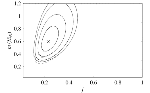
Figure 2: Likelihood contours for MACHO mass $m$ and Halo fraction $f$ for a typical spherical Halo. The contours enclose region of $34\%$, $68\%$, $90\%$, and $95\%$ probability. The cross shows the maximum-likelihood estimate. Two different curves are shown for each contour according to the velocity profile adopted for the sources: a Gaussian shape (solid line) and a universal VD (gray dotted line).

We found that the most probable mass for the Gaussian case is $m=0.60_{-0.33}^{+0.40}$ M_☉, where the errors are 68% confidence intervals, and $f=23\%$ with a $95\%$ confidence interval of $10\%-47\%$. We note that these values are slightly higher than, although fully compatible with, the original result reported by Alcock et al. (alcock00 (2000)). The mismatch is due to some differences in the modelling and the fact that the set of the events considered is smaller. If we consider that the velocities of the stars in the LMC are non-Gaussian-distributed, the likelihood contours have minimal differences from those of the previous case. We note that the most significant variation is in the estimate of the lens mass, but that this is not higher than $2\%$ for the $95\%$ probability contour line.

4 Discussion and conclusion

We have investigated the limits of the validity of the Gaussian approximation used to describe the kinematics of a source population in a microlensing context. This hypothesis, due to its practicality, has always been adopted without any check of its plausibility. We have remedied this deficiency in confirmation by an exhaustive analysis. To describe the motion of a stellar population with a non-spheroidal distribution as correctly as possible, we utilize two VDs (Sect. 2.1, Sect. 2.2) extracted from numerical simulations of collisionsless systems formed by self-gravitating particles. These VDs are substantially different than for a Gaussian one. We considered stars in the disk and bar components of the LMC and investigated their potential to be sources of lensing by transient lenses. In this framework, we recalculated the main microlensing parameters, including the MACHO halo fraction and the most likely value for the lens mass.

For a configuration in which the lenses and sources belong to the target galaxy, we detected an increase in the differential rate of microlensing events towards the LMC when we used a non-Gaussian VD to describe the motion of its stars instead of a Gaussian one. This increase is reflected in the estimate of the number of expected events, which is roughly $20\%$ higher than the 1.2 events found for the Gaussian case.

The prediction for a halo that consists entirely of MACHOs is a factor of $\sim 5$ above the observed rates. The situation does not change in a noticeable way if we consider a non-Gaussian VD, since we have found that the number of events expected is practically equal to the previous case. The results remain valid for both the DT and the universal VD. The main difference between the velocity dispersion of the LMC stars and the MACHOs, practically neutralizes any possible variation due to the different shape of the VD of the sources. The maximum-likelihood analysis provides values for $m$ and $f$ that are quite similar for the Gaussian and the non-Gaussian case. We conclude that the error in the estimate of the most probable value for the MACHO mass as well as for the Galactic halo fraction in the form of MACHOs, calculated with a Gaussian VD for the LMC sources, is roughly of the order of $1-2\%$. This fact implies that, in the study of the MW halo composition by microlensing, a Gaussian profile is a reasonable approximation for the velocity distribution of a system of source stars, even if they are not spherically distributed. On the other hand, for self-lensing, the Gaussian does not provide a good description of the kinematics of a non-spherically distributed stellar population, in a similar way to the disk or the bar of the LMC. To ensure accurate microlensing predictions, it is thus necessary to replace the Gaussian VD by a more physically motivated one, which takes into account the real spatial distribution of the source stars.

——————————————————————

References

- (1) Alcock, C., Allsman, R. A., Alves, D. R., et al. 2000, ApJ, 542, 281
- Assef et al. (2006) Assef, R. J., Gould, A., Afonso, C., et al. 2006, ApJ, 649, 954
- Bennett (2005) Bennett, D. P. 2005, ApJ, 633, 906
- Binney & Tremaine (1987) Binney, J., & Tremaine, S. 1987, Galactic Dynamics (Princeton Univ. Press)
- Binney & Merrifield (1998) Binney, J., & Merrifield, M. 1998, Galactic Astronomy (Princeton Univ. Press)
- Calchi Novati et al. (2005) Calchi Novati, S., Paulin-Henriksson, S., An, J., et al. 2005, A&A, 443, 911
- (7) Calchi Novati, S., De Luca, F., Jetzer, Ph., & Scarpetta G. 2006, A&A, 459, 407
- Chabrier (2001) Chabrier, G. 2001, A&A, 554, 1274
- de Jong et al. (2004) de Jong, J. T. A., Kuijken, K., Crots, A. P. S., et al. 2004, A&A, 417, 461
- de Rújula et al. (1995) de Rújula, A., Giudice, G. F., Mollerach, S., et al. 1995, MNRAS, 275, 545
- (11) Griest, K. 1991, ApJ, 366, 413
- (12) Hansen, S. H., Moore, B., Zemp, M., & Stadel J. 2006, JCAP, 01, 014
- (13) Iguchi, O., Sota, Y., Tatekawa, T., et al. 2005, Phys. Rev. E71, 016102
- Jetzer et al. (2002) Jetzer, Ph., Mancini, L., & Scarpetta, G. 2002, A&A, 393, 129
- (15) Mancini, L., Calchi Novati, S., Jetzer, Ph., & Scarpetta, G. 2004, A&A, 427, 61
- Navarro et al. (1996) Navarro, J. F., Frenk, C. S., & White, S. D. M. 1996, ApJ, 462, 563
- (17) Sackett, P. D., & Gould, A. 1993, ApJ, 419, 648
- Tisserand et al. (2007) Tisserand, P., Le Guillou, L., Afonso, C., et al. 2007, A&A, 469, 387
- van der Marel et al. (2002) van der Marel, R. P., Alves, D. R., Hardy, E., et al. 2002, AJ, 124, 2639
- Xue et al. (2008) Xue, X.-X., Rix, H.-W., Zhao, G., et al. 2008, ApJ, 684, 1143