Local Turbulence Simulations for the Multiphase ISM

Abstract

In this paper we show results of numerical simulations for the turbulence in the interstellar medium. These results were obtained using a Riemann solver-free numerical scheme for high-Mach number hyperbolic equations. Here we especially concentrate on the physical properties of the ISM. That is, we do not present turbulence simulations trimmed to be applicable to the interstellar medium. The simulations are rather based on physical estimates for the relevant parameters of the interstellar gas. Applying our code to simulate the turbulent plasma motion within a typical interstellar molecular cloud, we investigate the influence of different equations of state (isothermal and adiabatic) on the statistical properties of the resulting turbulent structures. We find slightly different density power spectra and dispersion maps, while both cases yield qualitatively similar dissipative structures, and exhibit a departure from the classical Kolmogorov case towards a scaling described by the She-Leveque model. Solving the full energy equation with realistic heating/cooling terms appropriate for the diffuse interstellar gas, we are able to reproduce a realistic two-phase distribution of cold and warm plasma. When extracting maps of polarised intensity from our simulation data, we find encouraging similarity to actual observations. Finally, we compare the actual magnetic field strength of our simulations to its value inferred from the rotation measure. We find these to be systematically different by a factor of about 1.5, thus highlighting the often underestimated influence of varying line-of-sight particle densities on the magnetic field strength derived from observed rotation measures.

1 Motivation

Interstellar space is filled by a dilute partially ionised gas called the Interstellar Medium (ISM). In contrast to the classical belief that it is a more or less undisturbed multi-phase medium existing in pressure equilibrium, the ISM is nowadays thought to be in a turbulent state (see, e. g., Elmegreen & Scalo, 2004). There are several hints for this turbulence coming from observations as are for example the broadening of spectral lines, the chemical mixing of the ISM and, indirectly, also the star formation rate (see, e. g., Elmegreen & Scalo, 2004; Scalo & Elmegreen, 2004). While turbulence in the latter case was accounted for simply by considering a turbulent pressure, a global description of the ISM has to take the turbulence directly into account (see, e. g., Larson, 1981; Lizano & Shu, 1989; Elmegreen, 1993).

While turbulence is certainly important on the largest scales, also atomic particles are thought to be strongly influenced by the turbulent fluctuations: The variability of the gas and of the electromagnetic field within are the means by which cosmic ray particles are scattered during their motion through the Galaxy and the intergalactic medium. The properties of the turbulence needed to calculate the diffusion lengths and similar quantities for these particles can, however, not be directly obtained from observations. Lacking the possibility to bring a probe into interstellar space in the near future (see, e. g., Fichtner et al., 2006, for the far-future prospects), observations using different parts of the electromagnetic spectrum are the only method to gain such information. So far, however, the observational access to fundamental turbulent quantities in the ISM is very limited. Due to the fact that also analytical models for turbulence are still lacking – at least for a system as complex as the ISM – we have to rely on numerical means to gain some insight into interstellar turbulence. Fortunately, the advance of computational resources allows even such complex systems as the ISM to be modelled numerically in the fluid description. It has, however, to be kept in mind that the ISM is not just an arbitrary plasma laboratory for the turbulence scientist. Even though the ISM shows a wide range of parameters, these parameters are interrelated in characteristic ways. Therefore, one has to properly prescribe the physical parameters of the corresponding simulations. In contrast to basic turbulence research simulations for example, one has to choose the external driving in accordance with the observations. Also heating and cooling processes usually have to be taken into account. In this connection numerical simulations are an interesting method to derive the influence of turbulence on the temperature of the ISM.

An additional complication arises by the fact that most parts of the ISM are highly compressible, thus allowing for the possibility of shocks to form in the turbulent plasma (see, e. g., Boldyrev et al., 2002). With this and the requirement for high spatial resolution, the demands on a numerical solver are very high. For this work we used an implementation of a conservative, central finite-volume scheme, which we demonstrate to be very suited for the complex task at hand. By way of this scheme we perform simulations for the ISM turbulence, which are adapted to the interstellar medium.

The structure of this paper is as follows. First, we discuss the physical description of the turbulent ISM. In the subsequent section we introduce the scheme used for this modelling. Finally, we show first results of the code’s application to interstellar turbulence.

2 The Physical Model

In this work we concern ourselves with the structure and fluctuations of the ISM. For this we first need to find a suitable physical description. Naturally, we will not consider a model describing the individual particles when dealing with the large gas masses in interstellar space. Even though the gas is very dilute, we will consider such large volumes that such a description is not necessary. Due to the limited computational resources, we will also not use a kinetic description. Therefore, we will rely on a fluid description for the interstellar plasma.

Consequently the ISM will be described by the ideal MHD equations:

$$\frac{\partial\rho}{\partial t}+\nabla\cdot\left(\rho\vec{u}\right) =0$$ (1)

$$\frac{\partial\left(\rho\vec{u}\right)}{\partial t}+\nabla\cdot\left(\rho\vec{u}\vec{u}\right)+\nabla\cdot\mathsf{P}+\frac{1}{\mu_{0}}\vec{B}\times\left(\nabla\times\vec{B}\right) =0$$ (2)

$$\frac{\partial\vec{B}}{\partial t}+\nabla\cdot\left(\vec{u}\vec{B}-\vec{B}\vec{u}\right) =0$$ (3)

$$\frac{\partial e}{\partial t}+\nabla\cdot\left(\left(e+\frac{B^{2}}{2\mu_{0}}+\mathsf{P}\cdot\right)\vec{u}-\frac{1}{\mu_{0}}\left(\vec{u}\cdot\vec{B}\right)\vec{B}\right) =$$ (4)

$$\qquad\qquad\qquad\qquad\qquad n_{\mathrm{H}}\Gamma-n_{\mathrm{H}}^{2}\Lambda+\nabla\cdot\left(\kappa\nabla T\right)$$

The relevant quantities are the mass density $\rho$, the flow velocity $\vec{u}$, the magnetic induction $\vec{B}$, and the overall energy density $e$. For the pressure tensor $\mathsf{P}$ we assume a description via a scalar pressure to be sufficient, thus, yielding $\mathsf{P}=p\hat{1}$, where $\hat{1}$ is the unit matrix. The source terms of the energy equation are the heating ($\Gamma$) and cooling functions ($\Lambda$), which both depend on the density and the temperature – here $n_{\mathrm{H}}$ is the hydrogen number density. Finally $\kappa$ is the constant coefficient of heat conduction, which was only included, when also heating and cooling terms were present to avoid unresolved growth of the thermal instability on the grid scale (see Koyama & Inutsuka, 2004). This was chosen as $\kappa=5\cdot 10^{-4}$ in normalised units.

The above equations are the compressible form of the MHD equations – allowing for the formation of shock structures as they are observed in the ISM (see, e. g., Vestuto et al., 2003). As an additional condition, we also have to fulfil

$$\nabla\cdot\vec{B}=0$$ (5)

at all times of the simulation. With these equations we possess the general framework for the simulation of the interstellar plasma. As mentioned above, however, there are several issues which have to be taken into account in addition to the fluid description of the plasma.

2.1 Implications of the Phase Structure

One of the most important issues setting the ISM apart from a turbulence laboratory is connected to the classical concept of its phase structure. From observations, it is known that the ISM consists of at least three distinct phases, being brought about by unstable regions in the pressure curve for the ISM. These result from an equilibrium of heating and cooling processes in the ISM. The resulting stable phases are characterised by some typical density and temperature (which, however, might vary quite strongly). This structure also allows for two basically different simulation scenarios.

On the one hand one could try to capture the multi-phase interstellar medium, whereas on the other hand only a small volume of the ISM could be taken into account, which would then reside exclusively in one of the phases. The latter option, thus, allows for a simplification of the above system of equations. The simplest possibility to describe one of the phases would be to investigate an isothermal medium, which just possesses the average temperature of the corresponding phase. In this case the evolution equation for the energy density (4) can be replaced by the following equation of state in order to close the system of equations:

$$p=c_{\mathrm{iso}}^{2}\rho\qquad\textnormal{with}\qquad c_{\mathrm{iso}}=\sqrt{\frac{k_{\mathrm{B}}T_{0}}{m_{0}}}.$$ (6)

Here $k_{\mathrm{B}}$ indicates the Boltzmann constant, $m_{0}$ is the reduced mass of a particle of the ISM, and $T_{0}$ is the temperature of the corresponding phase.

When investigating several phases at the same time, use of the full energy equation is mandatory. To allow for the existence of the phase structure, in this case, we have to include the corresponding heating and cooling functions for the ISM. For temperatures up to $10^{4.2}$ K we use the most general form for the cooling function given as:

$$\Lambda(x,T)=\sum_{i}\frac{n_{X_{i}}}{n_{H}}\left[x\lambda_{\mathrm{e}}(X_{i},T)+\lambda_{\mathrm{H}}(X_{i},T)\right]$$ (7)

Here the individual cooling functions $\lambda_{\mathrm{H}}(X_{i},T)$ and $\lambda_{\mathrm{e}}(X_{i},T)$ are given for the individual species $X_{i}$ in Penston (1970) and Dalgarno & McCray (1972) analytically. The resulting cooling rate depends on the fractional ionisation $x=n_{\mathrm{e}}/n_{\mathrm{H}}$ and the relative elemental abundances $n_{i}/{n_{\mathrm{H}}}$, which were also taken from Dalgarno & McCray (1972). For higher temperatures we use the approximate cooling function suggested in Gerritsen & Icke (1997) For the element abundances we use the depleted values from Kopp & Shchekinov (2007) with the exception of Oxygen, for which $X_{O}=8.53\cdot 10^{-4}$.

With regard to heating processes we only take the heating by external UV radiation incident onto the interstellar dust grains into account (see Bakes & Tielens, 1994). Other heating processes are thought to be negligible for the major part of the ISM (see Wolfire et al., 1995). The energy absorbed by the dust grains is transfered to the gas by collisions with the dust particles. Bakes & Tielens (1994) give for the corresponding heating rate of the interstellar gas:

$$n_{\mathrm{H}}\Gamma=1.0\cdot 10^{-25}n\ \varepsilon\ G_{0}\ \textnormal{J}\ \textnormal{m}^{-3}\ \textnormal{s}^{-1}$$ (8)

Here $\varepsilon$ is the fraction of FUV radiation absorbed by the dust grains, that is converted to the heating of the gas and is mainly determined by the neutral fraction of the gas under consideration. This fraction is estimated by Bakes & Tielens as:

$$\varepsilon=\frac{4.9\cdot 10^{-2}}{1+96\left(G_{0}T^{1/2}/n_{\mathrm{e}}\right)^{0.73}}+\frac{3.7\cdot 10^{-2}(T/10^{4}\textnormal{K})^{0.7}}{1+2\cdot 10^{2}\left(G_{0}T^{1/2}/n_{\mathrm{e}}\right)}$$ (9)

Here we assume that the strength of the FUV average interstellar radiation is $G_{0}=1.7$ times the estimate by Habing (1968) of $f_{\gamma}=1.6\cdot 10^{-6}\textnormal{J}\ \textnormal{m}^{-2}\ \textnormal{s}^{-1}$. From the combination of the above heating and cooling functions we computed the thermal equilibrium curve shown in Fig. 1. There the thermal pressure for thermal equilibrium is given as a function of the hydrogen number density.

Figure 1: Thermal pressure $p$ versus hydrogen number density $n_{\mathrm{H}}$ for the thermal equilibrium resulting from the heating and cooling functions used in this work. For details see the text.

At this point, we have to keep in mind that we can only consider the two low temperature phases of the ISM (the cold and the warm phase). A hot phase could be described by properly incorporating ionisation of the plasma. This, however, can not be done when using a single magnetised fluid.

Even when using a polytropic equation of state $p\propto\rho^{\gamma}$ instead of the full energy equation, there arises a slight difficulty. Namely, we have to make sure that the prescribed kinetic energy input for the driving is in the correct ratio to the thermal energy in the chosen phase of the ISM.

2.2 The Driving Process

Due to the very nature of turbulence, energy that is injected at some scale is transformed to fluctuations of ever smaller scale, until the dissipation range is reached, at which they are finally transformed into heat. Thus, a process is needed which constantly replenishes the energy that is lost at the dissipation scales, to maintain a specific level of the turbulence. For the ISM there are several plausible sources for this energy, of which supernovae seem to be the most important ones.

For large-scale simulations it would be feasible to include such driving directly into the simulations as artificial explosions (see, e. g., de Avillez & Breitschwerdt, 2004). For local simulations as they are performed here, however, this cannot be done. Therefore, we include a driving process, which affects only the largest spatial scales. On the one hand, that allows for a study of the turbulent cascade, which is not disturbed by the driving. On the other hand, this even allows for a plausible physical interpretation: The fluctuations represent the cascade continuing from scales larger than the computational domain.

The fluctuations are added as a velocity field with random amplitude and phases. This velocity field is chosen to be incompressible in order to mimic the transport through the inertial range from scales larger than the numerical domain to the largest scales under investigation. The amplitudes, however, do depend on the wave-number $\vec{k}$, by a dependence of the variance of the corresponding normally distributed random numbers on $\vec{k}$. By this, the average velocity power spectrum of the driving is given by:

$$E(k)=k^{4}\sigma^{2}_{\delta\vec{u}}(k)$$ (10)

where $\sigma_{\delta\vec{u}}(k)$ is the scale dependent standard deviation of the amplitude of the velocity disturbance. For the present simulations we selected a driving spectrum with $E(k)\propto k^{-1}$. Further details of the implementation of the driving process are given in appendix B.

For turbulence research a high energy input of fluctuations would be desirable. For the ISM, however, this is constrained by the actual physical values. If, e. g., supernovae are assumed to be the sources for the driving, there is an upper limit for the average input rate of kinetic energy into the system. Taking into account the overall energy output of a supernova explosion of $E\simeq 10^{43}$ – $10^{44}$ J (see, e. g., Dyson & Williams, 1997), the efficiency of conversion into kinetic energy, the volume of the galactic gaseous phase $V_{Gas}\simeq 1.4\cdot 10^{11}$ pc³, and the frequency of the explosions (one supernova per century – see de Avillez, 2000), we arrive at a base value of about $S_{\mathrm{e}}\simeq 10^{-27}\textnormal{ J m}^{-3}\textnormal{s}^{-1}$. This value may not be a strict upper limit, but it should not be abandoned arbitrarily. The actual values used in this work will be given when discussing the simulations.

2.3 Further Issues

One additional property, which is important for the ISM, is the compressibility of the gas. This allows for the existence of different kinds of shock waves. All of these have to be captured correctly by the numerical method used for the simulations. The important issue is that only conservative codes have been demonstrated to yield the correct speed and structure for the different kinds of discontinuities (see, e. g., Leveque, 2002). Also the steep gradients occurring at such structures must not induce any artificial fluctuations, which would be indiscernible from the turbulent ones.

Another issue is connected to the minimum simulation time. Classically it might seem necessary to simulate for several sound crossing times to allow for a signal propagation through the whole computational domain. Here, however, we will be investigating highly supersonic turbulence. Thus, the speed of sound is not a good tracer for the propagation time of features in the medium anymore. Instead the relevant timescale is the large eddy turnover time. For saturated turbulence this is given by (see Frisch, 1995):

$$\tau=\frac{L}{\textnormal{v}_{0}}\quad\textnormal{with}\quad L=\frac{M\textnormal{v}_{0}^{3}}{\epsilon}\quad\textnormal{and}\quad\textnormal{v}_{0}=\left(\frac{2}{3}\frac{E}{M}\right)^{1/2}$$ (11)

where $E$ is the overall energy and $M$ is the overall mass in the numerical domain and $\epsilon$ is the overall dissipation rate. The resulting values of $L$ and $\textnormal{v}_{0}$ can be interpreted as the typical size and the typical (rotational) velocity of an eddy, respectively.

3 Numerical Approach

There are several important demands for a numerical scheme for the simulation of the turbulent ISM. A basic requirement is a sufficiently high Reynolds number to actually allow the system to become turbulent. This is especially the case for the very high Reynolds numbers present in the ISM – corresponding to an extent of the turbulence spectrum of some ten orders of magnitude (see, e. g., Armstrong et al., 1995). Even though such a simulation will not be possible for years to come, the available simulations still have to yield very high Reynolds numbers.

While this can – for comparatively inefficient codes – be remedied by a sufficiently high spatial resolution, the high Mach number of the plasma in some phases of the ISM is an even more important demand. The corresponding supersonic flow in the ISM leads to the generation of shocks (see, e. g., de Avillez & Breitschwerdt, 2004), which have to be handled correctly by the numerical scheme. Especially, when investigating the turbulent fluctuations there must not be any spurious oscillations at shocks, which could not be disentangled from the turbulence itself. Many schemes, which are able to correctly reproduce such discontinuities are, however, of very low order, thus gaining little from high spatial resolution.

So far, only few algorithms for numerical MHD computations are in use for studying problems in the ISM. For two-dimensional studies see for example Passot et al. (1995), while for three-dimensional ones see Vestuto et al. (2003), Cho & Lazarian (2003), Balsara et al. (2001), Brandenburg & Dobler (2002) and Maron & Goldreich (2001), the latter of which considers only an incompressible velocity field. Some do not really meet the above requirements, others seem to have some additional problems (see, e. g., Falle, 2002). Here we apply our implementation of a Riemann solver-free central scheme, which is shown to reproduce the occurring shocks quite nicely (Essential features of this scheme are summarised in Appendix B). For this scheme the Reynolds number for the ideal MHD simulations can be estimated as $Re\simeq 3\cdot 10^{4}$ and $Re\simeq 1\cdot 10^{5}$ for the simulations with 256 and 512 grid-points in each of the spatial dimensions, respectively (see also Kissmann, 2006, for an estimate of the Reynolds numbers).

One feature of the code, which must not be forgotten, is its conservative property. This is especially of interest for turbulence simulations, because only using a conservative code yields the possibility to extract meaningful information about the energy content of the turbulence. For compressible MHD simulations in general, however, the conservation of the quantities is even more important, since only then a correct representation of the frequently occurring shock waves can be assured.

4 Simulations

In this work we are interested in the spatial and spectral structure of ISM turbulence. Due to the nature of the ISM it is a highly demanding task to achieve both of these goals. Whenever the whole structure of the ISM is considered, a global simulation would be necessary. This, however, would not supply information about the turbulence spectrum for individual part of the ISM. When one concentrates, in contrast, on local patches of the ISM, it is easily forgotten that one still has to take all the properties of the ISM into account, which were mentioned in the introduction.

Here we present results of our numerical simulations that were obtained for rather local models. In this work we investigate two basic scenarios. First, we discuss our simulation results for molecular cloud turbulence. Thereby we show the suitability of the scheme for simulations of compressible turbulence. In this case we investigate the influence of different equations of state on the statistical and spatial structure of the turbulence

Second, we take the phase structure of the ISM into account. We show local simulations for turbulence, for which the influence of heating and cooling processes leads to a two-phase medium.

5 Molecular Clouds

Interstellar turbulence is often discussed in the context of molecular clouds. This might seem arbitrary at first, but there are good reasons to concern ourselves with these ISM structures. First, they are very important for the dynamics of the ISM, since star formation takes place in just these regions. Second, a far more trivial reason to investigate turbulence in molecular clouds is that parts of the can be assumed to be of lower complexity than other regions of the ISM. This is due to the fact that typically the gas in molecular clouds is shielded from the interstellar radiation field. Therefore, ionisation and dissociation by UV photons can safely be neglected for a study of molecular clouds. This means that also external heating is of no importance in these regions.

The subtype of molecular cloud that we are investigating in this work is what Snow & McCall (2006) call the diffuse molecular clouds. These are already sufficiently isolated from the interstellar radiation field. The ionisation is, however, still sufficiently high so that the magnetic field can strongly influence the plasma and, therefore, must not be neglected. Despite the fact that chemistry already plays a role in these regions it is not as complex as in the dense cloud cores. Moreover, the number densities being of the order of $10^{8}$ particles per cubic meter are still low enough that self-gravity can be neglected. With a typical ionisation fraction of 0.01 in these molecular cloud regions, the initial electron density is $n_{\mathrm{e}}\simeq 10^{6}$ m^-3. It can also be shown that collisions of neutral and ionised particles are so frequent that a near perfect coupling of both particle species is achieved (see Kissmann, 2006). Therefore, ideal MHD is still a viable description for this environment.

The corresponding value for the temperature in these simulations is obtained from a model for the two-phase ISM. From the discussion in Cox (2005) we find a thermal pressure of about $7.76\cdot 10^{-14}$ Pa meaning that we are dealing with a temperature of about 56 K corresponding to a sound speed of 480 m s^-1 when we assume an average ion mass of $m_{0}=2m_{\mathrm{p}}$. The latter choice reflects the fact that hydrogen occurs partly in the form of neutral hydrogen molecules and that heavier elements are also present in the ISM (see, e. g., Snow & McCall, 2006). For the molecular clouds we use an energy input rate of $1\cdot 10^{-26}$ J m^-3 s^-1 corresponding to the fact that on average supernova explosions are expected to occur near or even within these structures. Finally, we choose a plasma $\beta$ of 0.3 corresponding to the observations (see, e. g., Kissmann, 2006), with the initially homogeneous magnetic field pointing into the $x$-direction.

The time is given in units of the sound crossing time through the simulation box, which is a cube with a side-length of $L_{\mathrm{B}}=$ 40 parsecs with periodic boundaries. In these units we drive the system with an input of kinetic fluctuations on scales $1\leq kL_{\mathrm{B}}/2\pi\leq 3$, where $k$ is the wave-number. Adding the velocity fluctuations every $\Delta t_{\mathrm{Drive}}=10^{-3}$ we ran the simulations in full turbulence for more than three eddy turnover times.

The results shown below were obtained with a resolution of $512$ cells in each of the three spatial directions, corresponding to a spatial resolution of less then 0.1 pc per cell. Here, we mainly investigate the influence of different equations of state onto the spatial structure and the statistics of the turbulence, where we will start with the former of those in the next section.

5.1 The Spatial Structure

The most obvious – and most directly accessible part of the spatial structure – is the density distribution. The amount of radiation emitted by a small volume of the ISM scales in general with its temperature and density. Therefore, for our isothermal simulations the density is the best tracer of how the medium would look like using different telescopes. The corresponding line-of-sight integral of the electron density is given as:

$$D_{M}=\int n_{\mathrm{e}}d\ l$$ (12)

As an example we show a comparison of this dispersion measure $D_{M}$ for the fully turbulent state for both a polytropic and an isothermal equation of state in Figs. 2 and 3.

Figure 2: Logarithm of the dispersion measure of the plasma in the numerical domain in units of $4\cdot 10^{-5}$ pc m^-3. Results are shown for a polytropic index of $\gamma=5/3$.

Figure 3: Same as Fig 2 but for an isothermal medium.

There the results are given for an adiabatic index of $\gamma=5/3$ in Fig. 2 and for an isothermal plasma in Fig. 3. All differences in these images can be attributed to the equation of state, since the driving in both cases was identical. This is reflected in the global similarities. Locally, however, the contrast in the images for the isothermal medium is much higher. This is due to the fact that for a polytropic equation of state structures get smoothed due to the higher pressure.

This fact is also reflected in the power spectra of the density fluctuations shown in Fig. 4 in a direct comparison for both cases. For the isothermal spectrum there is apparently much more power in the high wave-number modes of the mass density fluctuations corresponding to the small spatial scales. Obviously, however, not only the highest wave-numbers are influenced by the different choices for the equation of state. The fluctuations in the inertial range also differ.

Figure 4: Density power spectra for molecular cloud turbulence. Here the normalised density fluctuation power multiplied by $k^{0.45}$ as a function of wave-number $k$ is shown for the adiabatic and the isothermal case.

The fact that the density fluctuation spectrum is much shallower than the one reported in Armstrong et al. (1995) can be understood by a selection effect regarding the observations. Other authors (see, e. g., Deshpande et al., 2000) report different power laws for different phases of the ISM. It is also investigated by Kim & Ryu (2005), how this power law index depends on the Mach number of the medium. Our results shown in Fig. 4 are consistent with these latter results, where the authors also find a small power law index for high Mach numbers.

One important aspect of the spatial structure is the distribution of shocks because they are thought to have a direct influence on the statistics of the turbulence. This is, e. g., reflected in the model for the structure functions by She & Leveque (1994). This model indicates that the exponents of the structure functions – and, thus, the index of the power law of the velocity power spectrum – depend on the dimensionality of the dissipative structures.

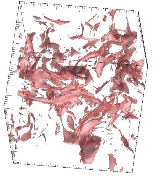
Figure 5: Isosurface plots for the square of the normalised current density. Results are shown for the isothermal case.

As an example we show in Fig. 5 the distribution of current sheets for the isothermal medium. Even though this plot differs from that for the adiabatic case (not shown), the essential information remains identical. The dissipative structures are current sheets. Thus, the fluctuation spectrum is dominated by two-dimensional structures in both cases. This leads, according to the model by She & Leveque (1994), to the expectation that the spectrum and also the structure functions should by identical to the bounds of numerical accuracy.

5.2 Statistics

Figure 6: Exponents for the structure functions as a function of order $n$ obtained using the extended self-similarity. Here data points for the isothermal medium are given in black, whereas the results for the adiabatic medium are shown in red. The latter are shifted a little to the right to enhance visibility. The data are given together with the corresponding error bars. Additionally, we show the theoretical prediction by Boldyrev et al. (2002) as the solid line and the Kolmogorov (1941) as the dotted line.

The statistics of the turbulence is shown here in the form of the velocity structure functions in Fig. 6. Here we investigate the parallel structure functions $S_{n}(l)$:

$$S_{n}(l)=\left<\left|\left(\vec{v}(\vec{r}+\vec{l})-\vec{v}(\vec{r})\right)\cdot\vec{e}_{l}\right|^{n}\right>\propto l^{\zeta_{n}}$$ (13)

with $\vec{e}_{l}=\vec{l}/l$ and $<>$ indicates an averaging over the spatial domain for one time-step. In Fig. 6 we give the exponents of these structure functions as a function of their order $n$. These were computed from a single time-step using the extended self-similarity (see Benzi et al., 1993). The latter must be invoked here, since the inertial range is not visible for the structure functions themselves. The statistics is quite good for the lower order structure functions. As can be seen from Fig. 6 the results are in good agreements to the theoretical prediction given in Boldyrev et al. (2002) for compressible MHD:

$$\frac{\zeta_{n}}{\zeta_{3}}=\frac{n}{9}+1-\left(\frac{1}{3}\right)^{n/3}$$ (14)

In particular it is obvious that the data do contradict the classical Kolmogorov scaling of $\zeta_{n}/\zeta_{3}=n/3$. Therefore, the results confirm the She & Leveque model. For both the isothermal and the adiabatic medium the spectral slope in the inertial range can be computed from the second-order structure function to be about $1.71$, which is just a little steeper than the classical Kolmogorov power law index.

Obviously there is no principal difference between the turbulence statistics of the isothermal and the adiabatic simulations. The structure functions are very similar for both cases. This is further evidence of the basic scaling structure. The shock structure might be different for isothermal or adiabatic systems, but the essential aspect of the She & Leveque model is the dimensionality of the dissipative structures. This is especially the case in ideal MHD, where shocks would have no extent in the shock direction if no numerical dissipation were present.

Concluding, we can say that the statistics of the turbulence does not depend on the equation of state used for the computations. There is, however, a strong dependence of the spatial structure as was seen in the preceding paragraph. Therefore, the equation of state has to be considered carefully whenever any resemblance to actual observations of molecular clouds is sought.

6 Diffuse Interstellar Gas

For the ISM, turbulence is mostly discussed for the context of molecular clouds. There are, however, also more global simulations for the interstellar medium of the Milky Way (see, e. g., de Avillez & Breitschwerdt, 2004; Breitschwerdt & de Avillez, 2006). These aim at a spatial domain reaching from the Galactic plane up into the halo of the Galaxy in order to investigate, e. g., the stratification of the interstellar medium. Here we are interested in similar simulations, however, on a local scale. In this paragraph, we will give our first results on such simulations, thus, showing the feasibility of the code for such simulations.

As was already mentioned above, the most important difference between molecular gas and the diffuse phase of the ISM is that the latter is influenced by the interstellar radiation field. This will be taken into account by the inclusion of an appropriate heating and cooling function for the diffuse ISM. Therefore, we solve the full energy equation with the additional source terms supplied by heating an cooling. In this case, in contrast to the simulations for the molecular clouds, we do not have to prescribe the correct temperature of the gas – this is instead achieved by heating and cooling processes. We have, however, to be careful to choose an initial condition from which the medium can evolve into a state possibly realised in nature. The hope that the initial state will independently evolve to a physically correct state is ruined, unfortunately, by the periodic boundary conditions. Due to these it is, e. g., not possible for high pressure regions to push anything out of the numerical domain – that is, the mass in the numerical domain will stay constant throughout the whole simulation. Therefore, the average pressure is just determined by the temperature.

This temperature will, at least on average, not exceed the value $10^{4}$ K due to the strongly increasing line cooling efficiency above this temperature. Thus, the initial density must be chosen sufficiently high, so that we end up with the correct pressure for the ISM. Due to the inclusion of the cooling function we will eventually end up with a dynamic equilibrium of a two-phase medium inherent in the cooling function. The initially homogeneous medium will be compressed into a dense, cold phase with a warm phase filling the space in between. The space filling factors of these phases will most probably depend on the initial density, with a lower density leading to a dominance of the warm phase, which we are essentially looking for.

By several numerical tests we arrived at a suitable initial density of $n_{0}=2\cdot 10^{6}$ m^-3, yielding physically reasonable results for the pressure distribution. Keeping in mind that the typical density of the warm H i gas is about $10^{5}$ m^-3, this allows for a fragmentation into a warm H i phase and a cold phase. The temperature was then initialised by the equilibrium value resulting from the heating-cooling equilibrium. With a side length of the numerical domain of 40 pc we apply an energy input rate of $S_{\mathrm{e}0}=5.3\cdot 10^{-27}$ J m^-3 s^-1. This rate was deliberately chosen to be moderately lower than the rate used for the molecular cloud simulations, because for those we expect the energy input into the turbulence to be higher than for the diffuse interstellar gas (DIG) due to the immediate presence of the sources of kinetic energy. Finally, the initial magnetic induction is set to about the same value as it was used for the molecular clouds.

The driving was implemented in the same way as for the molecular clouds. Here the simulations were performed on a grid of 256 cells in each of the spatial dimensions (due to the much higher numerical cost as compared to the molecular cloud simulations – this is mainly due to the sharp density contrast effected by the thermal instability, which results in a smaller time-step. Apart from that we had to let the simulations run for a longer time before a quasi-steady state was reached.). They were again evolved for several eddy turnover times (in this case we integrated up to 1.5 sound crossing times) after a saturated turbulent state was reached.

After the turbulence is fully developed the energy injected to maintain the turbulence is converted into heat at the small spatial scales, thus yielding a spatially non-homogeneous heating process. Thereby the average temperature of the medium increases to a value higher than the equilibrium temperature computed from the heating and cooling functions.

6.1 The Two-Phase Medium

As was expected our simulations indeed yielded a two-phase medium. Here the resulting temperature for the warm phase of the diffuse interstellar gas is of special interest due to the ongoing discussion about the heating processes for this phase of the ISM. As is illustrated in Reynolds (1995) and Reynolds et al. (1999) the heating process for the dilute ionised gas known as the diffuse interstellar gas or the warm ionised medium is not entirely clear yet. A possible solution of this problem was suggested in Minter & Spangler (1997) and was extended by Spanier & Schlickeiser (2005). The authors suggest the decay of interstellar plasma turbulence to be the main heating source for this environment.

The main shortcoming of these theoretical models is the fact that the authors had to use an analytical model for the turbulence spectrum. Therefore, the dissipation of the turbulence and the replenishing of the fluctuation energy in the energy range do not happen self-consistently. This could easily lead to incorrect results for the actual heating rate, when there is, e. g., too much energy in the model for the dissipation range. This is surely not the case for our numerical simulations. The results presented have, nonetheless, to be seen as a preliminary test for the study of the heating of the DIG. This is due to the fact that we use the well-documented cooling function for the warm H i gas, with a fixed degree of ionisation of 0.1, whereas major parts of the DIG have rather to be regarded as warm H ii. There is as yet, however, no analytical model available for the cooling of the warm H ii with a varying degree of ionisation – especially when using the single-fluid MHD equations. The best choice would, obviously, be the use of a multi-fluid model where ionisation and recombination are included, but such a model can not be solved using current numerical methods for a highly compressible medium.

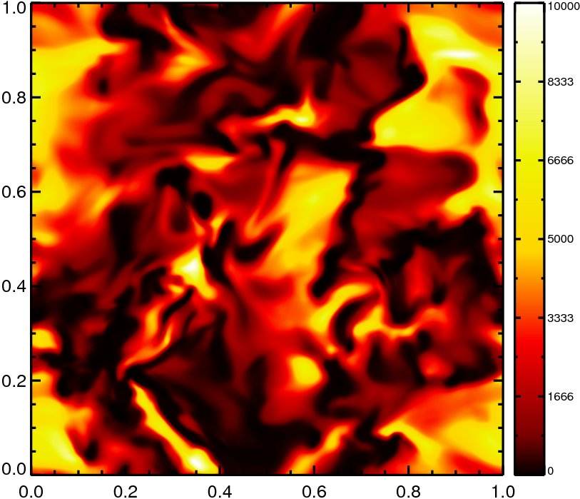
Figure 7: The temperature of the plasma in a slice through the computational domain given in Kelvins according to the colour-coding. Here the scale of the box is 40 pc.

Figure 8: Phase space distribution function for the whole computational domain. Obviously the unstable regime between the warm ($n<5.6$ m^-3) and the cold phase ($n>6.8$ m^-3) is significantly populated due to the turbulence.

The spatial temperature distribution as found from our simulations is visualised in Fig. 7. The computed ISM is dominated by a warm phase with temperatures of several thousand Kelvins. Regions containing this warm gas are separated by cool clouds with temperatures below 500 K. These can be identified as the typical molecular cloud structures. Thus, we have reproduced what is commonly known from observations – cool clouds embedded within a warm inter-cloud medium.

With regard to Fig. 7 there is apparently a certain spatial scale connected to the fluctuation in the numerical domain. This scale comes about by the thermal instability. It arises due to the fact that fluctuations with sufficiently short wavelength are stable against the thermal instability when their period is shorter than their cooling time, whereas fluctuations with long wavelength are unstable. Thus, there is an intermediate scale, for which the growth rate for the thermal instability is maximal. This scale can be estimated by the product of the cooling time with the typical wave speed. From the fast-mode speed we, thus, find a scale of $\sim$6.5 pc for the maximally growing modes, which is consistent with the impression from Fig. 7.

For a more direct analysis of the present phase structure we show the phase-space distribution in Fig. 8. Apparently the thermal equilibrium curve leaves its footprint in this distribution. While a warm phase with densities below $n\simeq 5.6$ m^-3 and a cool phase with densities above $n\simeq 6.8$ m^-3 are present it is, however, obvious that the unstable range is also significantly populated. This is due to the fact that the gas is driven into the unstable regime by the turbulence. For further discussions on the population of the unstable regime see also Sánchez-Salcedo et al. (2002)

6.2 Polarisation Canals

Apart from the two-phase structure, which is directly accessible to observations, there are also other quantities available to observers. One way to gain knowledge about the interstellar magnetic field is connected to the Faraday effect. The observational quantity in this context is the so-called rotation measure $R_{M}$. This can be accessed observationally, e. g., by an investigation of the polarised pulsar radiation. For simulations, this quantity can be accessed directly by integrating the data over the numerical domain.

Instead of the rotation measure, however, we will rather discuss the polarised intensity, which is closely connected to the former. We investigate a phenomenon found in several radio maps: elongated structures with very little polarised intensity with a width near that of the telescope beam – being usually referred to as canals (see, e. g., Fletcher & Shukurov, 2006). Basically they are thought to result at least partially from the finite resolution of the corresponding radio observations. Whenever the polarisation of the detected radiation changes over an area on the sky smaller than the beam of the telescope, these polarisation canals can occur.

Here we will investigate the possibility of the formation of these canals due to a foreground polarisation screen as suggested in Fletcher & Shukurov (2006). The other possible method for the formation of such canals discussed there – a formation due to differential Faraday rotation – is left for the future. Thus, we assume that homogeneously polarised radiation is produced in a region behind a foreground medium and is subject to Faraday rotation only in the latter. Strong gradients in this foreground Faraday screen result also in strong gradients in the Faraday rotation for radiation from the background. This then leads to the observed canals, whenever radiation of perpendicular polarisation occurs over the width of a telescope beam.

In this case the pattern of the observed canals strongly depends on the beam-width and also on the wavelength of the observed radiation. For the latter a too short wavelength means that the foreground Faraday rotation is too ineffective as to produce different polarisation angles. In contrast a too long wavelength causes complete depolarisation – even a slight difference in the rotation measure causes a huge difference in polarisation, so that the polarisation vectors become randomly distributed.

We computed the polarisation maps corresponding to our simulations using a similar procedure as introduced in Haverkorn & Heitsch (2004). From the rotation measure for the corresponding direction we first compute the local polarisation angle $\delta\theta$, which is given by:

$$\delta\theta(\lambda) =R_{M}\lambda^{2}$$ (15)

$$\textnormal{with}\qquad R_{M}=-\frac{e^{3}}{8\pi^{2}\varepsilon_{0}c^{3}m^{2}_{e}}\int_{0}^{l}n_{\mathrm{e}}(l^{\prime})B_{\parallel}(l^{\prime})\ dl^{\prime}$$

From this we then compute the Stokes parameters $Q$ and $U$:

$$U=\sin(2\delta\ \theta(\lambda))\quad\textnormal{and}\quad Q=\cos(2\delta\ \theta(\lambda))$$ (16)

By smoothing their maps using a Gaussian beam with a width of 2.5 grid cells we then mimic the beam width of the virtual telescope. From these smoothed maps $\tilde{U}$ and $\tilde{Q}$ we finally compute the polarised intensity:

$$I=\sqrt{\tilde{U}^{2}+\tilde{Q}^{2}}$$ (17)

Be aware that the results shown in Fig. 9 were computed for a medium in a box of an extent of only 40 parsecs. Unlike Haverkorn & Heitsch (2004) we did not stack several of the simulation boxes atop of each other in the direction under consideration with a shift in a perpendicular direction. We rather intend to use an adapted wavelength that yields canals in the polarised intensity. Whereas the wavelength used might not correspond to any of those used for actual observations, an artificial extension of the numerical domain would just yield similar results for a shorter wavelength. We, however, do not feel confident stacking shifted boxes atop of each other, because the shifts of the individual boxes against each other can lead to unphysical gradients at their interfaces.

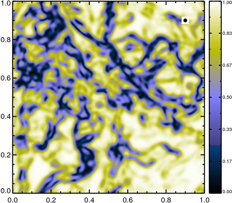
Figure 9: Normalised polarised intensity computed assuming a homogeneously polarised background radiation. The resulting intensity is computed with the plasma in the simulations being used as a foreground Faraday screen. The line-of-sight corresponds to the initial magnetic field direction. Results are shown for a wavelength, $\lambda$, of 0.3 m. The width of the artificial telescope beam is indicated as the black circle in the white box.

The polarised intensity map computed from our simulations is depicted in Fig. 9 for the directions along the initial magnetic field. We show the resulting intensity for a wavelength of $\lambda=0.3$ m best suited to visualise the polarisation canals. Interestingly, we had to choose a slightly different wavelength ($\lambda=0.4$ m) for the direction perpendicular to the magnetic field (not shown here). Obviously the gradients of the rotation measure in the direction of the initial magnetic field are stronger than the ones in the perpendicular direction. Therefore, the wavelength for this case had to be chosen a little shorter than for the other one. Apparently, it is possible to explain the depolarisation canals visible in radio observations by a foreground Faraday screen. There are obvious canals of just the width of the telescope beam. One has, however, to be careful with this statement: we found these canals only to become apparent in a very limited range of wavelengths. For actual observations it is highly improbable to observe just the appropriate wavelength range. Nonetheless, we see an encouraging similarity when we compare our results to actual observations (see, e. g., Shukurov & Berkhuijsen, 2003). Thus, it might be that the observed effect is due to the quite similar effect of the differential Faraday rotation.

Our results also look quite similar to those obtained by Haverkorn & Heitsch (2004). In contrast to their approach we used a physically correct representation of the warm phase of the ISM. Especially the Mach number chosen here is far more appropriate for the dilute plasma than the one used by these authors. Their statement that the turbulence cascade is very similar for the high Mach number and the low Mach number regime has to be considered with caution. One important point is that the spatial density structure has a huge influence on the rotation measure as will become clear later-on. Also, as was discussed in Kim & Ryu (2005) the density structure is very different for different Mach numbers. Consequently, one has to be very careful when using high Mach number simulations for the dilute ISM.

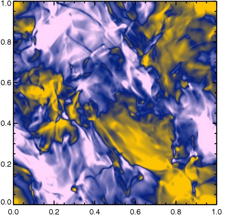
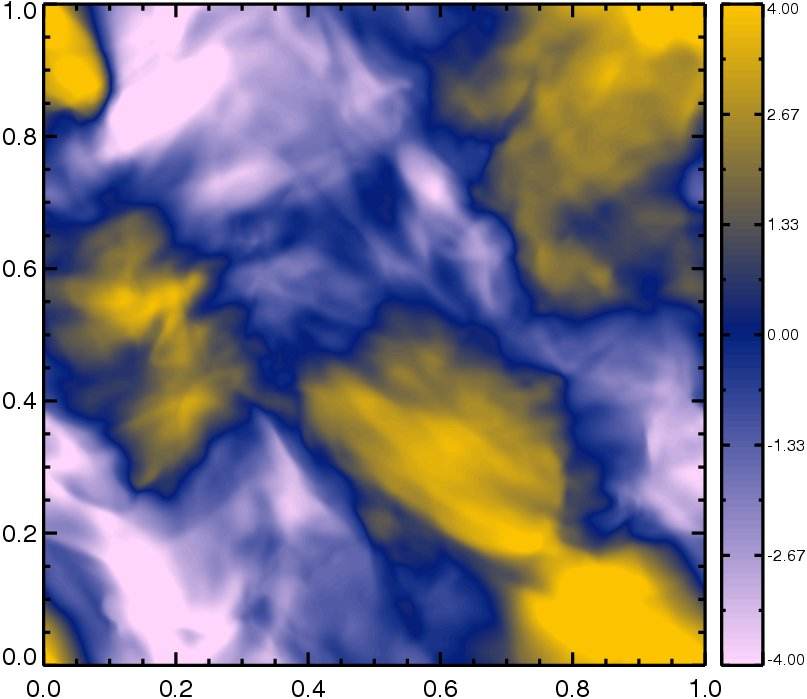
Figure 10: Comparison of the mass-weighted average for the normalised parallel magnetic induction (left) to the actual line-of-sight integral (right).

The latter statement is supported by what is displayed in Fig. 10, where the magnetic induction as inferred from the rotation and the dispersion measure is compared with the average magnetic induction along the same direction. Clearly the estimate differs significantly from the actual values - this shows the strong difference between the mass-weighted and the unweighted average. In particular we find that the mass-weighted average shows much more structure than is actually there. What is additionally apparent in Fig. 10 is that the absolute value of the magnetic induction is on average slightly overestimated as compared to the actual line-of-sight integral. This qualitative impression is confirmed by a quantitative analysis – on average the magnitude of the magnetic induction turns out to be higher by a factor of up to 1.15. This has to be taken into account whenever an interpretation of any observations is attempted. The reason for this discrepancy is the inhomogeneous mass distribution. For a completely homogeneous medium the rotation measure would directly yield the average magnetic induction. Obviously, the Mach number for the dilute phase of the ISM is still high enough to yield this strong discrepancy between the actual and the inferred magnetic field.

This result is another hint that one has to be careful to use the appropriate Mach numbers for the simulations of all the ISM phases. It also applies to the computation of the polarisation canals. Due to the fact that the rotation measure seems to depend strongly on the Mach number, one has to take care to use the appropriate simulations for the polarisation canals. It will be left as a task for the future to investigate how the deviation of the estimated magnetic field strength and also the structure of the canals depend on the average Mach number of the medium.

7 Conclusions

In this work we investigated basic turbulence theory in the framework of the interstellar medium. In many cases turbulence simulations are applied to the interstellar medium (ISM) merely because it is a medium with extremely high Reynolds numbers, and the parameters of the ISM are only taken into account as far as they are needed for the turbulence research. Here, however, we investigated basic turbulence properties, while at the same time we modelled the properties of the ISM as thoroughly as possible. The important point is that there are many physical processes operating in the ISM, which eventually should be incorporated in the corresponding simulations. These processes reach from external influences of the radiation field originating from hot stars to the internal interaction of the particles culminating in the intricate chemistry of the molecular cloud medium. Each of the different phases of the ISM has its own dominant processes to be taken into account for a realistic modelling.

In the present simulations we included heating and cooling where is was necessary. The resulting equations were then solved using a Riemann solver-free conservative finite-volume scheme. From the simulation results it becomes apparent that this scheme is suitable for the simulation of ISM turbulence. In this paper we investigated two different scenarios for the ISM turbulence. We simulated both an isothermal molecular cloud medium and the dilute phase of the ISM.

For the former we demonstrated that the turbulence in our molecular cloud simulations is in accord with most recent models for compressible MHD turbulence. We find the dissipative structures in our simulations to be mainly two-dimensional. Shocks and current sheets make the major contribution to the damping of the turbulent fluctuations. From the computed second-order structure function we can derive the power law index for the power spectrum of the velocity fluctuations. This is only slightly steeper than that for incompressible, homogeneous hydrodynamical turbulence, i. e., it remains considerably below 2 for all cases. Therefore, this exponent is comfortably far away from what was classically thought to be a special value for particle transport theories (see, e. g., Schlickeiser, 1988).

Further, we investigated the consequences of using an isothermal and an adiabatic equation of state. While there are clear differences in the spatial structures, these do not extend to the statistics of the turbulence that can be characterised by structure functions. Only for the density power spectrum there are significant differences, where, however, simulations with still higher spatial resolutions are needed to clarify more details. It might be possible that these differences result from the smoother density structures of the adiabatic medium, which would sharpen for higher spatial resolutions.

Also for the warm phase of the ISM we could demonstrate that the numerical scheme is appropriate for simulations of this phase. The observed temperatures were found to be in the range known for the DIG. The warm gas surrounds in these simulations dense filaments of a cold gas, which corresponds to the typical molecular cloud parameters. This two-phase medium is, however, not in thermal pressure equilibrium. The ISM obviously has to be regarded as a very dynamic medium.

Finally, we discussed the rotation measure obtained from the numerical simulations. We could identify canals also seen in polarised intensity maps of the ISM found from radio observations. In this context we showed that it is important to use the correct Mach number in the simulations. Even for comparatively low Mach numbers for the WIM there can obviously result a significant deviation of the estimate of the magnetic field inferred from the observation of the rotation measure as compared to the actual magnetic field.

Acknowledgements

We would like to thank the anonymous referee for a timely and useful report. This work was partially financed by the Deutsche Forschungsgemeinschaft (DFG) through the Sonderforschungsbereich SFB 591 and benefitted from the Finnish-German cooperation funded via DAAD 313-SF-PPP Finnland. Computational resources were provided in the project hbo25 by the Forschungszentrum Jülich.

Appendix A The Numerical Solver

The hyperbolic part of the system of equations introduced in section 2 is solved using a multi-dimensional version of the semi-discrete central scheme introduced in Kurganov et al. (2001). This scheme was designed to yield highly accurate solutions of hyperbolic conservation laws of the general form:

$$\frac{\partial\mathbf{u}}{\partial t}+\nabla\cdot\mathsf{F}(\mathbf{u})=0$$ (18)

Here $\mathbf{u}$ is some vector quantity with $\mathsf{F}$ being a Flux-Tensor, which may also depend on $\mathbf{u}$. The resulting scheme is derived using an integration over parts of the individual numerical cells in order to obtain a numerical flux over the cell interfaces without the necessity to employ a Riemann solver. This together with a TVD (total variation diminishing) reconstruction of the point values at the cell interfaces from the resulting cell averages, yields a simple and robust numerical scheme, which suppresses spurious oscillations at steep gradients.

In the limit $t\to 0$ one approaches the so-called semi-discrete version of the scheme. In this limit the scheme can be written in the general form:

$$\frac{\partial\vec{u}_{i,j,k}}{\partial t}= \frac{\vec{H}^{x}_{i+1/2,j,k}-\vec{H}^{x}_{i-1/2,j,k}}{\Delta x}+\frac{\vec{H}^{y}_{i,j+1/2,k}-\vec{H}^{y}_{i,j-1/2,k}}{\Delta y}$$

$$+ \frac{\vec{H}^{z}_{i,j,k+1/2}-\vec{H}^{z}_{i,j,k-1/2}}{\Delta z}$$ (19)

where the fluxes are given by:

$$\vec{H}^{x}_{i+\frac{1}{2},j,k}= \frac{1}{a^{+}_{i+\frac{1}{2},j,k}+a^{-}_{i+\frac{1}{2},j,k}}$$ (20)

$$\times\left(a^{+}_{i+\frac{1}{2},j,k}\vec{f}(\vec{u}^{-}_{i+\frac{1}{2},j,k})-a^{-}_{i+\frac{1}{2},j,k}\vec{f}(\vec{u}^{+}_{i+\frac{1}{2},j,k})\right.$$

$$\quad-\left.a^{+}_{i+\frac{1}{2},j,k}a^{-}_{i+\frac{1}{2},j,k}\left(\vec{u}^{+}_{i+\frac{1}{2},j,k}-\vec{u}^{-}_{i+\frac{1}{2},j,k}\right)\right)$$

and similarly for $H^{y}$ and $H^{z}$. Here $a^{\pm}$ represent an upper limit for the maximum signal propagation velocity, $\vec{u}^{\pm}$ indicates the point values obtained using the reconstruction polynomial in the local ($-$) and in the next cell ($+$), respectively, and $\vec{f}$ denotes the corresponding physical fluxes. In the case of the MHD equations the maximum signal propagation velocity can be estimated to be the sum of the background flow velocity and the fast magneto-sonic speed.

To ensure the TVD property of the resulting scheme the point values $\vec{u}^{E/W}$ at the cell faces have to be estimated in a way as to be TVD. This is done via a reconstruction polynomial the order of which at the same time determines the order of the scheme. This reconstruction polynomial is chosen in a way as to fulfil the conservation properties – in particular we are using a second-order polynomial together with a minmod limiter (for a proof of the TVD property and a discussion of the minmod limiter see, e. g., Kurganov et al., 2001).
Remarks:

The order of the scheme is not only given by the order of the reconstruction polynomial. Also, the numerical approximation of the integral over the cell faces has to be at least of the same order. This was an additional motivation to use a second-order scheme, because for second-order the midpoint rule is still sufficient. For higher-order schemes the reconstruction, therefore, becomes much more expensive. Apart from that the order has to be reduced for higher-order schemes near any of the omnipresent shock waves in highly supersonic turbulence.

So far, we only have a scheme capable of solving hyperbolic equations. As we will see in the next section, the solenoidality of the magnetic field demands some additional effort.

The time evolution of the system of MHD equations is done via a Runge-Kutta method.

A.1 Divergence of the Magnetic Field

Whereas the analytical derivation of the MHD equations did consider the solenoidality of the magnetic field by application of the constraint:

$$\nabla\cdot\vec{B}=0$$ (21)

Eq. (3) does not maintain this constraint inherently. This leads to the problem that $|\nabla\cdot\vec{B}|$ increases with time, thus, rendering the solution unphysical.

Luckily, there are different ways to fulfil this condition numerically. Unfortunately only one of these could be shown to be suitable for the simulation of compressible turbulence. Especially the projection scheme proposed first by Chorin (1968) for the incompressibility constraint in the Navier-Stokes equations and later-on applied to plasma physics by Brackbill & Barnes (1980) proved to be not usable in the present context. This is due to the fact that there result some spurious oscillations at the smallest spatial scales, which strongly distort the spectrum (see also Kissmann, 2006). This leads to an obvious deviation of the spectrum in the dissipation range, which cannot be tolerated.

Therefore, we are using a constrained transport evolution of the scheme in order to assure the solenoidality of the field. This method proved to be highly efficient and does not produce numerical artifacts. See also in Evans & Hawley (1988) for a derivation of the scheme. The resulting scheme was extensively tested by Kissmann (2006) and was proved to fulfil all the requirements stated above.

Appendix B Implementation of the Driving Process

As was discussed above the driving process used in this work has to fulfil several important constraints: First the fluctuations have to be at large spatial scales. Then, the fluctuations have to be completely random, while the energy distribution over the different scales has to satisfy some form of scale dependence. Apart from that we only used a fully solenoidal velocity field to drive the fluctuations. Finally the overall energy of the fluctuations to be added to the velocity field has to correspond to some physical values (the supernova energy input rate in our case).

In this section we discuss the specific procedure that results in the random fluctuation field. We start by giving the random fluctuations in wave-number space – thus, we can restrict the fluctuations to large spatial scales. For this we worked closely along what is suggested in literature (see especially Vestuto et al., 2003; Christensson et al., 2001; Stone et al., 1998). The idea is to introduce fluctuations of random amplitude, with the amplitudes distributed according to a normal distribution on each of the input scales. The dependence of the fluctuation energy on the spatial scale is at the same time fixed by including a scale dependence of the variance $\sigma_{\delta\vec{u}}^{k}$ of the normal distribution. For a normal distribution around zero this just determines the width of the Gaussian $G_{\delta\vec{u},k}$. For the velocity fluctuations $\delta\textnormal{v}$ this means we have:

$$\left(\sigma_{\delta\vec{u}}^{k}\right)^{2}=\int\delta\vec{u}^{2}G_{\delta\vec{u},k}d^{3}\delta u\equiv\left<\delta\vec{u}(\vec{k})^{2}\right>$$ (22)

That is, in this case the variance is equivalent to the second-order moment of the velocity fluctuations at scale $k$. Thus, we fix the average form of the initial spectrum by prescribing the scale dependence of $\sigma_{\delta\vec{u}}^{k}$.

The next step is to transform the resulting field to configuration space. There we assure its solenoidality by taking the curl of the random field. This operation, however, also changes the slope in wave-number space. In particular we have:

$$\nabla\times\vec{A}(\vec{x})\quad\longrightarrow\quad\vec{k}\times\vec{A}(\vec{k})$$ (23)

This means that for the omni-directional spectrum there results an additional factor of $k$ for the spectral slope of the velocity power spectrum. An omni-directional energy spectrum is eventually obtained from the angle-integrated form of the square of the velocity – that is the velocity spectra resulting from the above differential operation have to be squared and multiplied by an additional factor of $k^{2}$ (the latter resulting from the angle integration). With all this in mind it is possible to set the wave-number dependence of the variance in a way as to provide any desired spectral slope. Fixing the wave-number dependence of the standard deviation, thus, yields a spectral slope of the form:

$$E(k)_{\mathrm{Init}}=k^{2}(k\ \sigma_{\delta\vec{u}}^{k})^{2}$$ (24)

From the corresponding inverse relation we find that if a random field with an average power law index of $-s$ is desired, the variance has to fulfil the relation:

$$\sigma_{\delta\vec{u}}\propto k^{-s/2-2}$$ (25)

Thus, the full procedure is to give the desired driving in wave-number space, at the same time restricting the spectrum only to small wave-numbers. After this the fluctuations are transformed into configuration space, where we only use their solenoidal part. Finally we determine the energy and the momentum added to the numerical domain from the resulting field. The former of these is the reduced to zero, whereas the latter is normalised to the desired overall input energy.

References

- Armstrong et al. (1995) Armstrong J. W., Rickett B. J., Spangler S. R., 1995, ApJ, 443, 209
- Bakes & Tielens (1994) Bakes E. L. O., Tielens A. G. G. M., 1994, ApJ, 427, 822
- Balsara et al. (2001) Balsara D., Ward-Thompson D., Crutcher R. M., 2001, MNRAS, 327, 715
- Benzi et al. (1993) Benzi R., Ciliberto S., Tripiccione R., Baudet C., Massaioli F., Succi S., 1993, Phys. Rev. E, 48, R29
- Boldyrev et al. (2002) Boldyrev S., Nordlund Å., Padoan P., 2002, ApJ, 573, 678
- Brackbill & Barnes (1980) Brackbill J. U., Barnes D. C., 1980, J. Comput. Phys., 35, 426
- Brandenburg & Dobler (2002) Brandenburg A., Dobler W., 2002, Computer Physics Communications, 147, 471
- Breitschwerdt & de Avillez (2006) Breitschwerdt D., de Avillez M. A., 2006, A&A, 452, L1
- Cho & Lazarian (2003) Cho J., Lazarian A., 2003, MNRAS, 345, 325
- Chorin (1968) Chorin A. J., 1968, Math. Comp., 22, 745
- Christensson et al. (2001) Christensson M., Hindmarsh M., Brandenburg A., 2001, Phys. Rev. E, 64, 056405
- Cox (2005) Cox D. P., 2005, ARA&A, 43, 337
- Dalgarno & McCray (1972) Dalgarno A., McCray R. A., 1972, ARA&A, 10, 375
- de Avillez & Breitschwerdt (2004) de Avillez M., Breitschwerdt D., 2004, Ap&SS, 292, 207
- de Avillez (2000) de Avillez M. A., 2000, MNRAS, 315, 479
- Deshpande et al. (2000) Deshpande A. A., Dwarakanath K. S., Goss W. M., 2000, ApJ, 543, 227
- Dyson & Williams (1997) Dyson J. E., Williams D. A., 1997, The physics of the interstellar medium. The physics of the interstellar medium. Edition: 2nd ed. Publisher: Bristol: Institute of Physics Publishing, 1997. Edited by J. E. Dyson and D. A. Williams. Series: The graduate series in astronomy. ISBN: 0750303069
- Elmegreen (1993) Elmegreen B. G., 1993, ApJ, 419, L29+
- Elmegreen & Scalo (2004) Elmegreen B. G., Scalo J., 2004, ARA&A, 42, 211
- Evans & Hawley (1988) Evans C. R., Hawley J. F., 1988, ApJ, 332, 659
- Falle (2002) Falle S. A. E. G., 2002, ApJ, 577, L123
- Fichtner et al. (2006) Fichtner H., Heber B., Leipold M., 2006, Astrophysics and Space Sciences Transactions, 2, 33
- Fletcher & Shukurov (2006) Fletcher A., Shukurov A., 2006, MNRAS, 371, L21
- Frisch (1995) Frisch U., 1995, Turbulence. The legacy of A.N. Kolmogorov. Cambridge: Cambridge University Press, —c1995
- Gerritsen & Icke (1997) Gerritsen J. P. E., Icke V., 1997, A&A, 325, 972
- Habing (1968) Habing H. J., 1968, Bull. Astron. Inst. Netherlands, 19, 421
- Haverkorn & Heitsch (2004) Haverkorn M., Heitsch F., 2004, A&A, 421, 1011
- Kim & Ryu (2005) Kim J., Ryu D., 2005, ApJ, 630, L45
- Kissmann (2006) Kissmann R., 2006, PhD thesis, Ruhr-Universität Bochum
- Kolmogorov (1941) Kolmogorov A. N., 1941, Dokl. Akad. Nauk. SSSR., 32, 16
- Kopp & Shchekinov (2007) Kopp A., Shchekinov Y. A., 2007, Physics of Plasmas, 14, 073701
- Koyama & Inutsuka (2004) Koyama H., Inutsuka S.-i., 2004, ApJ, 602, L25
- Kurganov et al. (2001) Kurganov A., Noelle S., Petrova G., 2001, SIAM J. Sci. Comput., 23, 707
- Larson (1981) Larson R. B., 1981, MNRAS, 194, 809
- Leveque (2002) Leveque Randall J., 2002, Finite Volume Methods for Hyperbolic Problems. Cambridge University Press
- Lizano & Shu (1989) Lizano S., Shu F. H., 1989, ApJ, 342, 834
- Maron & Goldreich (2001) Maron J., Goldreich P., 2001, ApJ, 554, 1175
- Minter & Spangler (1997) Minter A. H., Spangler S. R., 1997, ApJ, 485, 182
- Passot et al. (1995) Passot T., Vazquez-Semadeni E., Pouquet A., 1995, ApJ, 455, 536
- Penston (1970) Penston M. V., 1970, ApJ, 162, 771
- Reynolds (1995) Reynolds R. J., 1995, in Ferrara A., McKee C. F., Heiles C., Shapiro P. R., eds, ASP Conf. Ser. 80: The Physics of the Interstellar Medium and Intergalactic Medium Diffuse Optical Emission Lines as Probes of the Interstellar and Intergalactic Ionizing Radiation. pp 388–+
- Reynolds et al. (1999) Reynolds R. J., Haffner L. M., Tufte S. L., 1999, ApJ, 525, L21
- Sánchez-Salcedo et al. (2002) Sánchez-Salcedo F. J., Vázquez-Semadeni E., Gazol A., 2002, ApJ, 577, 768
- Scalo & Elmegreen (2004) Scalo J., Elmegreen B. G., 2004, ARA&A, 42, 275
- Schlickeiser (1988) Schlickeiser R., 1988, J. Geophys. Res., 93, 2725
- She & Leveque (1994) She Z.-S., Leveque E., 1994, Phys. Rev. Lett., 72, 336
- Shukurov & Berkhuijsen (2003) Shukurov A., Berkhuijsen E. M., 2003, MNRAS, 342, 496
- Snow & McCall (2006) Snow T. P., McCall B. J., 2006, ARA&A, 44, 367
- Spanier & Schlickeiser (2005) Spanier F., Schlickeiser R., 2005, A&A, 436, 9
- Stone et al. (1998) Stone J. M., Ostriker E. C., Gammie C. F., 1998, ApJ, 508, L99
- Vestuto et al. (2003) Vestuto J. G., Ostriker E. C., Stone J. M., 2003, ApJ, 590, 858
- Wolfire et al. (1995) Wolfire M. G., Hollenbach D., McKee C. F., Tielens A. G. G. M., Bakes E. L. O., 1995, ApJ, 443, 152