Langevin Thermostat for Rigid Body Dynamics

Ruslan L. Davidchack    Richard Handel    M.V. Tretyakov Department of Mathematics, University of Leicester, Leicester, LE1 7RH, United Kingdom
Abstract

We present a new method for isothermal rigid body simulations using the quaternion representation and Langevin dynamics. It can be combined with the traditional Langevin or gradient (Brownian) dynamics for the translational degrees of freedom to correctly sample the NVT𝑁𝑉𝑇NVT distribution in a simulation of rigid molecules. We propose simple, quasi-symplectic second-order numerical integrators and test their performance on the TIP4P model of water. We also investigate the optimal choice of thermostat parameters.

I Introduction

Classical molecular dynamics simulation of an isolated system naturally samples states from a microcanonical (NVE𝑁𝑉𝐸NVE) ensemble, where the number of particles N𝑁N, volume V𝑉V, and total energy of the system E𝐸E are held constant. However, in many cases it is desirable to study the system in a more experimentally relevant canonical (NVT𝑁𝑉𝑇NVT) ensemble, where the temperature T𝑇T is specified instead of E𝐸E. In order to sample from the canonical ensemble, the molecular dynamics equations of motion are modified by introducing the interaction of the system with a “thermostat”. There exist a large variety of approaches for introducing such a thermostat, which can be roughly classified into two categories: deterministic and stochastic, depending on whether the resulting equations of motion contain a random component (for a review, see, e.g. Ref. Hunenberger05, ).

Among various deterministic approaches, those based on coupling the system to a few external degrees of freedom (e.g. Nosé-Hoover thermostat) have become very popular. Given ergodicity in the molecular system dynamics, such thermostats are proven to generate correct canonical ensemble sampling of the system phase space. However, since the thermostat variables are coupled and control directly only global system quantities (e.g. kinetic energy), such thermostats rely on the efficient energy transfer within the system to achieve equipartition within the canonical distribution, such that the average energy of each degree of freedom within the system is equal to kBTsubscript𝑘𝐵𝑇k_{B}T. Therefore, in a system where the energy transfer between its different parts is slow (e.g., systems combining fast and slow degrees of freedom), the simple Nosé-Hoover thermostat may have difficulty maintaining the same temperature for the different parts of the system. In this case more complicated thermostats are necessary, for example, Nosé-Hoover chain thermostat, or separate thermostats for different parts of the systems (see, e.g. Ref. Ben, ).

The stochastic approach exploits ergodic stochastic differential equations (SDEs) with the Gibbsian (canonical ensemble) invariant measure. For this purpose, Langevin-type equations or gradient systems with noise can be used (see, e.g. Refs. SKE99, ; ISK01, ; Soize, ; Stua, ; MT7, and references therein). Stochastic thermostats, with their independent thermalization of each degree of freedom, provide direct control of equipartition and thus do not need to rely on the efficient energy transfer within the system.

In order to achieve such a direct thermalization of the system, one needs to be able to apply stochastic thermostats to all types of degrees of freedom. The standard Langevin equations for translational degrees of freedom are well known, while Langevin thermostats for systems with constraints have been proposed quite recently Eijnden06 ; Sun08 . In this paper we introduce Langevin equations for the rigid body dynamics in the quaternion representation and propose effective second-order quasi-symplectic numerical integrators for their simulation. These equations can be coupled either with Langevin or Brownian dynamics for the translational degrees of freedom.

In Section II we recall the Hamiltonian system for rigid body dynamics in the quaternion representation from Ref. qua02, , based on which we derive Langevin and gradient-Langevin thermostats. Second-order (in the weak sense) numerical methods for these stochastic systems are constructed in Section III. We test the thermostats and the proposed numerical integrators on the TIP4P model of waterJorgensen83 . The results of our numerical experiments are presented in Section IV. In particular, we investigate the optimal choice of thermostat parameters and the discretization error of the numerical methods. A summary of the obtained results is given in Section V.

II Equations of Motion

We consider a system of n𝑛n rigid three-dimensional molecules described by the center-of-mass coordinates 𝐫=(r1𝖳,,rn𝖳)𝖳3n,𝐫superscriptsuperscript𝑟1𝖳superscript𝑟𝑛𝖳𝖳superscript3𝑛\mathbf{r}=(r^{1\mathsf{T}},\ldots,r^{n\,\mathsf{T}})^{\mathsf{T}}\in\mathbb{R}^{3n}, rj=(r1j,r2j,r3j)𝖳3,superscript𝑟𝑗superscriptsuperscriptsubscript𝑟1𝑗superscriptsubscript𝑟2𝑗superscriptsubscript𝑟3𝑗𝖳superscript3r^{j}=(r_{1}^{j},r_{2}^{j},r_{3}^{j})^{\mathsf{T}}\in\mathbb{R}^{3}, and the rotational coordinates in the quaternion representation 𝐪=(q1𝖳,,qn𝖳)𝖳4n𝐪superscriptsuperscript𝑞1𝖳superscript𝑞𝑛𝖳𝖳superscript4𝑛\mathbf{q}=(q^{1\,\mathsf{T}},\ldots,q^{n\,\mathsf{T}})^{\mathsf{T}}\in\mathbb{R}^{4n}, qj=(q0j,q1j,q2j,q3j)𝖳4,superscript𝑞𝑗superscriptsuperscriptsubscript𝑞0𝑗superscriptsubscript𝑞1𝑗superscriptsubscript𝑞2𝑗superscriptsubscript𝑞3𝑗𝖳superscript4q^{j}=(q_{0}^{j},q_{1}^{j},q_{2}^{j},q_{3}^{j})^{\mathsf{T}}\in\mathbb{R}^{4}, such that |qj|=1superscript𝑞𝑗1|q^{j}|=1. We use standard matrix notations, and “𝖳𝖳{\mathsf{T}}” denotes transpose. Following Ref. qua02, , we write the system Hamiltonian in the form

H(𝐫,𝐩,𝐪,𝝅)=𝐩𝖳𝐩2m+j=1nl=13Vl(qj,πj)+U(𝐫,𝐪),𝐻𝐫𝐩𝐪𝝅superscript𝐩𝖳𝐩2𝑚superscriptsubscript𝑗1𝑛superscriptsubscript𝑙13subscript𝑉𝑙superscript𝑞𝑗superscript𝜋𝑗𝑈𝐫𝐪H(\mathbf{r},\mathbf{p},\mathbf{q},\bm{\pi})=\frac{\mathbf{p}^{\mathsf{T}}\mathbf{p}}{2m}+\sum_{j=1}^{n}\sum_{l=1}^{3}V_{l}(q^{j},\pi^{j})+U(\mathbf{r},\mathbf{q}), (1)

where 𝐩=(p1𝖳,,pn𝖳)𝖳3n𝐩superscriptsuperscript𝑝1𝖳superscript𝑝𝑛𝖳𝖳superscript3𝑛\mathbf{p=}(p^{1\,\mathsf{T}},\ldots,p^{n\,\mathsf{T}})^{\mathsf{T}}\in\mathbb{R}^{3n}, pj=(p1j,p2j,p3j)𝖳3,superscript𝑝𝑗superscriptsuperscriptsubscript𝑝1𝑗superscriptsubscript𝑝2𝑗superscriptsubscript𝑝3𝑗𝖳superscript3p^{j}=(p_{1}^{j},p_{2}^{j},p_{3}^{j})^{\mathsf{T}}\in\mathbb{R}^{3}, are the center-of-mass momenta conjugate to 𝐫𝐫\mathbf{r}, 𝝅=(π1𝖳,,πn𝖳)𝖳4n𝝅superscriptsuperscript𝜋1𝖳superscript𝜋𝑛𝖳𝖳superscript4𝑛\bm{\pi}=(\pi^{1\,\mathsf{T}},\ldots,\pi^{n\,\mathsf{T}})^{\mathsf{T}}\in\mathbb{R}^{4n}, πj=(π0j,π1j,π2j,π3j)𝖳4,superscript𝜋𝑗superscriptsuperscriptsubscript𝜋0𝑗superscriptsubscript𝜋1𝑗superscriptsubscript𝜋2𝑗superscriptsubscript𝜋3𝑗𝖳superscript4\pi^{j}=(\pi_{0}^{j},\pi_{1}^{j},\pi_{2}^{j},\pi_{3}^{j})^{\mathsf{T}}\in\mathbb{R}^{4}, are the angular momenta conjugate to 𝐪𝐪\mathbf{q}, and U(𝐫,𝐪)𝑈𝐫𝐪U(\mathbf{r},\mathbf{q}) is the potential interaction energy. The second term represents the rotational kinetic energy of the system with

Vl(q,π)=18Il[π𝖳Slq]2,q,π4,l=1,2,3,formulae-sequencesubscript𝑉𝑙𝑞𝜋18subscript𝐼𝑙superscriptdelimited-[]superscript𝜋𝖳subscript𝑆𝑙𝑞2𝑞formulae-sequence𝜋superscript4𝑙123V_{l}(q,\pi)=\frac{1}{8I_{l}}\left[\pi^{\mathsf{T}}S_{l}q\right]^{2},\ \ q,\pi\in\mathbb{R}^{4},\ \ l=1,2,3, (2)

where the three constant 444-by-444 matrices Slsubscript𝑆𝑙S_{l} are such that

S1q=(q1,q0,q3,q2)𝖳,subscript𝑆1𝑞superscriptsubscript𝑞1subscript𝑞0subscript𝑞3subscript𝑞2𝖳\displaystyle S_{1}q=(-q_{1},q_{0},q_{3},-q_{2})^{\mathsf{T}},\!\! S2q=(q2,q3,q0,q1)𝖳,subscript𝑆2𝑞superscriptsubscript𝑞2subscript𝑞3subscript𝑞0subscript𝑞1𝖳\displaystyle\!\!S_{2}q=(-q_{2},-q_{3},q_{0},q_{1})^{\mathsf{T}},
S3qsubscript𝑆3𝑞\displaystyle S_{3}q =\displaystyle= (q3,q2,q1,q0)𝖳,superscriptsubscript𝑞3subscript𝑞2subscript𝑞1subscript𝑞0𝖳\displaystyle(-q_{3},q_{2},-q_{1},q_{0})^{\mathsf{T}},

and Ilsubscript𝐼𝑙I_{l} are the principal moments of inertia of the rigid molecule. The Hamilton equations of motion are

d𝐫dt=𝐩m,d𝐩dt=𝐫U(𝐫,𝐪),dqjdt=l=13πjVl(qj,πj),dπjdt=l=13qjVl(qj,πj)qjU(𝐫,𝐪),j=1,,n.\begin{split}\frac{d\mathbf{r}}{dt}&=\frac{\mathbf{p}}{m}\,,\quad\frac{d\mathbf{p}}{dt}=-\nabla_{\mathbf{r}}U(\mathbf{r},\mathbf{q})\,,\\ \frac{dq^{j}}{dt}&=\sum_{l=1}^{3}\nabla_{\pi^{j}}V_{l}(q^{j},\pi^{j})\,,\\ \frac{d\pi^{j}}{dt}&=-\sum_{l=1}^{3}\nabla_{q^{j}}V_{l}(q^{j},\pi^{j})-\nabla_{q^{j}}U(\mathbf{r},\mathbf{q})\,,\\ j&=1,\ldots,n\,.\end{split} (3)

It is easy to check that if the initial conditions are chosen such that |qj(0)|=1superscript𝑞𝑗01|q^{j}(0)|=1, then the corresponding Hamilton equations of motion ensure that

|qj(t)|=1,j=1,,n,for all t0.formulae-sequencesuperscript𝑞𝑗𝑡1formulae-sequence𝑗1𝑛for all 𝑡0|q^{j}(t)|=1\,,\ \ j=1,\ldots,n\,,\ \ \mbox{for all~{}}t\geq 0. (4)

In the rest of this section we derive stochastic thermostats for this molecular system, which preserve (4). They take the form of ergodic SDEs with the Gibbsian (canonical ensemble) invariant measure possessing the density

ρ(𝐫,𝐩,𝐪,𝝅)exp(βH(𝐫,𝐩,𝐪,𝝅)),proportional-to𝜌𝐫𝐩𝐪𝝅𝛽𝐻𝐫𝐩𝐪𝝅\rho(\mathbf{r},\mathbf{p},\mathbf{q},\bm{\pi})\varpropto\exp(-\beta H(\mathbf{r},\mathbf{p},\mathbf{q},\bm{\pi})), (5)

where β=1/(kBT)>0𝛽1subscript𝑘𝐵𝑇0\beta=1/(k_{B}T)>0 is an inverse temperature.

II.1 Langevin-type equations

Consider the Langevin-type equations (in the form of Ito)111Following the standard notation of the SDE theory, we use capital letters to denote the SDE solution and small letters for the initial data and for corresponding “dummy” variables.

dRj𝑑superscript𝑅𝑗\displaystyle dR^{j} =\displaystyle= Pjmdt,Rj(0)=rj,superscript𝑃𝑗𝑚𝑑𝑡superscript𝑅𝑗0superscript𝑟𝑗\displaystyle\frac{P^{j}}{m}dt,\ \ R^{j}(0)=r^{j}, (6)
dPj𝑑superscript𝑃𝑗\displaystyle dP^{j} =\displaystyle= rjU(𝐑,𝐐)dtsubscriptsuperscript𝑟𝑗𝑈𝐑𝐐𝑑𝑡\displaystyle-\nabla_{r^{j}}U(\mathbf{R},\mathbf{Q})dt
γg(Pj,Rj)dt+b(Rj)dwj(t),Pj(0)=pj,𝛾𝑔superscript𝑃𝑗superscript𝑅𝑗𝑑𝑡𝑏superscript𝑅𝑗𝑑superscript𝑤𝑗𝑡superscript𝑃𝑗0superscript𝑝𝑗\displaystyle-\gamma g(P^{j},R^{j})dt+b(R^{j})dw^{j}(t),\ \ P^{j}(0)=p^{j},
dQj𝑑superscript𝑄𝑗\displaystyle dQ^{j} =\displaystyle= l=13πjVl(Qj,Πj)dt,Qj(0)=qj,|qj|=1,formulae-sequencesuperscriptsubscript𝑙13subscriptsuperscript𝜋𝑗subscript𝑉𝑙superscript𝑄𝑗superscriptΠ𝑗𝑑𝑡superscript𝑄𝑗0superscript𝑞𝑗superscript𝑞𝑗1\displaystyle\sum_{l=1}^{3}\nabla_{\pi^{j}}V_{l}(Q^{j},\Pi^{j})dt,\ \ Q^{j}(0)=q^{j},\ \ |q^{j}|=1,
dΠj𝑑superscriptΠ𝑗\displaystyle d\Pi^{j} =\displaystyle= l=13qjVl(Qj,Πj)dtqjU(𝐑,𝐐)dtsuperscriptsubscript𝑙13subscriptsuperscript𝑞𝑗subscript𝑉𝑙superscript𝑄𝑗superscriptΠ𝑗𝑑𝑡subscriptsuperscript𝑞𝑗𝑈𝐑𝐐𝑑𝑡\displaystyle-\sum_{l=1}^{3}\nabla_{q^{j}}V_{l}(Q^{j},\Pi^{j})dt-\nabla_{q^{j}}U(\mathbf{R},\mathbf{Q})dt
\displaystyle- ΓG(Qj,Πj)dt+B(Qj,Πj)dWj(t),Πj(0)=πj,Γ𝐺superscript𝑄𝑗superscriptΠ𝑗𝑑𝑡𝐵superscript𝑄𝑗superscriptΠ𝑗𝑑superscript𝑊𝑗𝑡superscriptΠ𝑗0superscript𝜋𝑗\displaystyle\!\!\Gamma G(Q^{j},\Pi^{j})dt+B(Q^{j},\Pi^{j})dW^{j}(t),\ \ \Pi^{j}(0)=\pi^{j},
j𝑗\displaystyle j =\displaystyle= 1,,n,1𝑛\displaystyle 1,\ldots,n,

where γ0𝛾0\gamma\geq 0 and Γ0Γ0\Gamma\geq 0 with γΓ>0𝛾Γ0\gamma\Gamma>0 are the friction coefficients for the translational and rotational motions, respectively, measured in units of inverse time, which control the strength of coupling of the system to the “heat bath”; g𝑔g is a 333-dimensional appropriately normalized vector; G𝐺G is a 444-dimensional vector, which provides a balance in coupling various rotational degrees of freedom with the “heat bath”; b𝑏b and B𝐵B are 333-by-333 and 444-by-444 matrices, respectively; and (𝐰𝖳,𝐖𝖳)𝖳=(w1𝖳,,wn𝖳,W1𝖳,,Wn𝖳)𝖳superscriptsuperscript𝐰𝖳superscript𝐖𝖳𝖳superscriptsuperscript𝑤1𝖳superscript𝑤𝑛𝖳superscript𝑊superscript1𝖳superscript𝑊𝑛𝖳𝖳(\mathbf{w}^{\mathsf{T}},\mathbf{W}^{\mathsf{T}})^{\mathsf{T}}=(w^{1\,\mathsf{T}},\ldots,w^{n\,\mathsf{T}},W^{1^{{}^{\mathsf{T}}}},\ldots,W^{n\,\mathsf{T}})^{\mathsf{T}} is a (3n+4n)3𝑛4𝑛(3n+4n)-dimensional standard Wiener process with wj=(w1j,w2j,w3j)𝖳superscript𝑤𝑗superscriptsuperscriptsubscript𝑤1𝑗superscriptsubscript𝑤2𝑗superscriptsubscript𝑤3𝑗𝖳w^{j}=(w_{1}^{j},w_{2}^{j},w_{3}^{j})^{\mathsf{T}} and Wj=(W0j,W1j,W2j,W3j)𝖳.superscript𝑊𝑗superscriptsuperscriptsubscript𝑊0𝑗superscriptsubscript𝑊1𝑗superscriptsubscript𝑊2𝑗superscriptsubscript𝑊3𝑗𝖳W^{j}=(W_{0}^{j},W_{1}^{j},W_{2}^{j},W_{3}^{j})^{\mathsf{T}}.

For simplicity, we assumed here that g𝑔g, G𝐺G, b𝑏b, and B𝐵B are the same for all n𝑛n molecules, although one could choose them depending on the molecule number j𝑗j. The latter can be especially useful for systems consisting of significantly different types of molecules. It is also natural to require that each degree of freedom is thermalized by its own independent noise, and in what follows we assume that the matrices b𝑏b and B𝐵B are diagonal. Further, we suppose that the coefficients of (6)-(II.1) are sufficiently smooth functions and the process X(t)=(𝐑𝖳(t),𝐏𝖳(t),𝐐𝖳(t),𝚷𝖳(t))𝖳𝑋𝑡superscriptsuperscript𝐑𝖳𝑡superscript𝐏𝖳𝑡superscript𝐐𝖳𝑡superscript𝚷𝖳𝑡𝖳X(t)=(\mathbf{R}^{\mathsf{T}}(t),\mathbf{P}^{\mathsf{T}}(t),\mathbf{Q}^{\mathsf{T}}(t),\mathbf{\Pi}^{\mathsf{T}}(t))^{\mathsf{T}} is ergodic, i.e., there exists a unique invariant measure μ𝜇\mu of X𝑋X and independently of x14n𝑥superscript14𝑛x\in\mathbb{R}^{14n} there exists the limit

limtEφ(X(t;x))=φ(x)𝑑μ(x):=φergsubscript𝑡𝐸𝜑𝑋𝑡𝑥𝜑𝑥differential-d𝜇𝑥assignsuperscript𝜑𝑒𝑟𝑔\lim_{t\rightarrow\infty}E\varphi(X(t;x))=\int\varphi(x)\,d\mu(x):=\varphi^{erg} (8)

for any function φ(x)𝜑𝑥\varphi(x) with polynomial growth at infinity (see Refs. Has, ; Soize, ; Stua, ; Tal02, and references therein). Here X(t;x)𝑋𝑡𝑥X(t;x) is the solution X(t)𝑋𝑡X(t) of (6)-(II.1) with the initial condition X(0)=X(0;x)=x.𝑋0𝑋0𝑥𝑥X(0)=X(0;x)=x.

It is not difficult to see that the solution of (6)-(II.1) preserves the property (4), i.e.,

|Qj(t)|=1,j=1,,n,for all t0.formulae-sequencesuperscript𝑄𝑗𝑡1formulae-sequence𝑗1𝑛for all 𝑡0|Q^{j}(t)|=1,\ \ j=1,\ldots,n\,,\ \ \mbox{for all~{}}t\geq 0. (9)

Now we find relations between γ𝛾\gamma, ΓΓ\Gamma, g𝑔g, G𝐺G, b𝑏b, and B𝐵B such that the invariant measure μ𝜇\mu is Gibbsian with the density (5). The density ρ(𝐫,𝐩,𝐪,𝝅)𝜌𝐫𝐩𝐪𝝅\rho(\mathbf{r},\mathbf{p},\mathbf{q},\bm{\pi}) should satisfy the stationary Fokker-Planck equation:

Lρ=0,superscript𝐿𝜌0L^{\ast}\rho=0, (10)

where

Lρ:=j=1n{i=13bii2(rj)22ρ(pij)2+i=14122(πij)2(Bii2(qj,πj)ρ)+pj[γg(pj,rj)ρ]qj(πjl=13Vl(qj,πj)ρ)+πj[(qjl=13Vl(qj,πj)+qjU(𝐫,𝐪)+ΓG(qj,πj))ρ]}1m𝐫(𝐩ρ)+𝐩[𝐫U(𝐫,𝐪)ρ].assignsuperscript𝐿𝜌superscriptsubscript𝑗1𝑛superscriptsubscript𝑖13superscriptsubscript𝑏𝑖𝑖2superscript𝑟𝑗2superscript2𝜌superscriptsuperscriptsubscript𝑝𝑖𝑗2superscriptsubscript𝑖1412superscript2superscriptsuperscriptsubscript𝜋𝑖𝑗2superscriptsubscript𝐵𝑖𝑖2superscript𝑞𝑗superscript𝜋𝑗𝜌subscriptsuperscript𝑝𝑗delimited-[]𝛾𝑔superscript𝑝𝑗superscript𝑟𝑗𝜌subscriptsuperscript𝑞𝑗subscriptsuperscript𝜋𝑗superscriptsubscript𝑙13subscript𝑉𝑙superscript𝑞𝑗superscript𝜋𝑗𝜌subscriptsuperscript𝜋𝑗delimited-[]subscriptsuperscript𝑞𝑗superscriptsubscript𝑙13subscript𝑉𝑙superscript𝑞𝑗superscript𝜋𝑗subscriptsuperscript𝑞𝑗𝑈𝐫𝐪Γ𝐺superscript𝑞𝑗superscript𝜋𝑗𝜌1𝑚subscript𝐫𝐩𝜌subscript𝐩delimited-[]subscript𝐫𝑈𝐫𝐪𝜌\begin{split}L^{\ast}\rho&:=\sum_{j=1}^{n}\Biggl{\{}\sum_{i=1}^{3}\frac{b_{ii}^{2}(r^{j})}{2}\frac{\partial^{2}\rho}{\bigl{(}\partial p_{i}^{j}\bigr{)}^{2}}+\sum_{i=1}^{4}\frac{1}{2}\frac{\partial^{2}}{\bigl{(}\partial\pi_{i}^{j}\bigr{)}^{2}}\left(B_{ii}^{2}(q^{j},\pi^{j})\rho\right)+\nabla_{p^{j}}\cdot\left[\gamma g(p^{j},r^{j}\mathbf{)}\rho\right]-\nabla_{q^{j}}\cdot\left(\nabla_{\pi^{j}}\sum_{l=1}^{3}V_{l}(q^{j},\pi^{j})\rho\right)\\ &\left.+\nabla_{\pi^{j}}\cdot\left[\left(\nabla_{q^{j}}\sum_{l=1}^{3}V_{l}(q^{j},\pi^{j})+\nabla_{q^{j}}U(\mathbf{r},\mathbf{q})+\Gamma G(q^{j},\pi^{j})\right)\rho\right]\right\}-\frac{1}{m}\nabla_{\mathbf{r}}\cdot(\mathbf{p}\rho)+\nabla_{\mathbf{p}}\cdot\left[\nabla_{\mathbf{r}}U(\mathbf{r},\mathbf{q})\rho\right].\end{split}

After some calculations, we get the required relations:

βmbii22[βm(pij)21]+γgipijγβmgipij=0𝛽𝑚superscriptsubscript𝑏𝑖𝑖22delimited-[]𝛽𝑚superscriptsuperscriptsubscript𝑝𝑖𝑗21𝛾subscript𝑔𝑖superscriptsubscript𝑝𝑖𝑗𝛾𝛽𝑚subscript𝑔𝑖superscriptsubscript𝑝𝑖𝑗0\frac{\beta}{m}\frac{b_{ii}^{2}}{2}\left[\frac{\beta}{m}\bigl{(}p_{i}^{j}\bigr{)}^{2}-1\right]+\gamma\frac{\partial g_{i}}{\partial p_{i}^{j}}-\gamma\frac{\beta}{m}g_{i}p_{i}^{j}=0 (11)

and

βBii22[β(Hπij)22H(πij)2]+(Biiπij)2+Bii2Bii(πij)2βBiiBiiπijHπij+ΓGiπijΓβGiHπij=0.\begin{split}\beta\frac{B_{ii}^{2}}{2}&\Biggl{[}\beta\biggl{(}\frac{\partial H}{\partial\pi_{i}^{j}}\biggr{)}^{2}-\frac{\partial^{2}H}{\bigl{(}\partial\pi_{i}^{j}\bigl{)}^{2}}\Biggr{]}+\biggl{(}\frac{\partial B_{ii}}{\partial\pi_{i}^{j}}\biggr{)}^{2}\\ &+B_{ii}\frac{\partial^{2}B_{ii}}{\bigl{(}\partial\pi_{i}^{j}\bigr{)}^{2}}-\beta B_{ii}\frac{\partial B_{ii}}{\partial\pi_{i}^{j}}\frac{\partial H}{\partial\pi_{i}^{j}}\\ &+\Gamma\frac{\partial G_{i}}{\partial\pi_{i}^{j}}-\Gamma\beta G_{i}\frac{\partial H}{\partial\pi_{i}^{j}}=0.\end{split} (12)

Since numerical methods are usually simpler for systems with additive noise, we limit computational consideration of thermostats in this paper to the case of biisubscript𝑏𝑖𝑖b_{ii} and Biisubscript𝐵𝑖𝑖B_{ii} both being constant. At the same time, we note that general thermostats (6)-(II.1) with (11)-(12) may have some beneficial features for certain systems but we leave this question for further study. For constant biisubscript𝑏𝑖𝑖b_{ii} and Bii,subscript𝐵𝑖𝑖B_{ii}, the relations (11)-(12) take the form

γgi(pj,rj)=βmbii22pijand ΓGi(qj,πj)=βBii22Hπij.formulae-sequence𝛾subscript𝑔𝑖superscript𝑝𝑗superscript𝑟𝑗𝛽𝑚superscriptsubscript𝑏𝑖𝑖22superscriptsubscript𝑝𝑖𝑗and Γsubscript𝐺𝑖superscript𝑞𝑗superscript𝜋𝑗𝛽superscriptsubscript𝐵𝑖𝑖22𝐻superscriptsubscript𝜋𝑖𝑗\gamma g_{i}(p^{j},r^{j}\mathbf{)}=\frac{\beta}{m}\frac{b_{ii}^{2}}{2}p_{i}^{j}\ \ \text{and\ \ }\Gamma G_{i}(q^{j},\pi^{j})=\beta\frac{B_{ii}^{2}}{2}\frac{\partial H}{\partial\pi_{i}^{j}}.

In the considered molecular model it is natural to have the same value for all biisubscript𝑏𝑖𝑖b_{ii}, i=1,2,3,𝑖123i=1,2,3, and the same value for all Biisubscript𝐵𝑖𝑖B_{ii}, i=1,,4.𝑖14i=1,\ldots,4. Further, taking into account the form of the Hamiltonian (1) and that

πl=13Vl(q,π)subscript𝜋superscriptsubscript𝑙13subscript𝑉𝑙𝑞𝜋\displaystyle\nabla_{\pi}\sum_{l=1}^{3}V_{l}(q,\pi) =\displaystyle= 14l=131Il[π𝖳Slq]Slq14superscriptsubscript𝑙131subscript𝐼𝑙delimited-[]superscript𝜋𝖳subscript𝑆𝑙𝑞subscript𝑆𝑙𝑞\displaystyle\frac{1}{4}\sum_{l=1}^{3}\frac{1}{I_{l}}\left[\pi^{\mathsf{T}}S_{l}q\right]S_{l}q
=\displaystyle= 14l=131IlSlq[Slq]𝖳π,14superscriptsubscript𝑙131subscript𝐼𝑙subscript𝑆𝑙𝑞superscriptdelimited-[]subscript𝑆𝑙𝑞𝖳𝜋\displaystyle\frac{1}{4}\sum_{l=1}^{3}\frac{1}{I_{l}}S_{l}q\left[S_{l}q\right]^{\mathsf{T}}\pi,

we can write

G(q,π)=J(q)πandBii2=2MΓβformulae-sequence𝐺𝑞𝜋𝐽𝑞𝜋andsuperscriptsubscript𝐵𝑖𝑖22𝑀Γ𝛽G(q,\pi)=J(q)\pi\ \ \text{and}\ \ B_{ii}^{2}=\frac{2M\Gamma}{\beta}

with

J(q)=l=131IlSlq[Slq]𝖳l=131Iland M=4l=131Il.formulae-sequence𝐽𝑞superscriptsubscript𝑙131subscript𝐼𝑙subscript𝑆𝑙𝑞superscriptdelimited-[]subscript𝑆𝑙𝑞𝖳superscriptsubscript𝑙131subscript𝐼𝑙and 𝑀4superscriptsubscript𝑙131subscript𝐼𝑙J(q)=\frac{\sum_{l=1}^{3}\frac{1}{I_{l}}S_{l}q\left[S_{l}q\right]^{\mathsf{T}}}{\sum_{l=1}^{3}\frac{1}{I_{l}}}\ \ \text{and\ \ }M=\frac{4}{\sum_{l=1}^{3}\frac{1}{I_{l}}}. (13)

Note that TrJ(q)=|q|2=1.T𝑟𝐽𝑞superscript𝑞21\mathop{\mathrm{T}r}J(q)=|q|^{2}=1.

Thus, in this paper under ‘Langevin thermostat’ we understand the following stochastic system

dRj𝑑superscript𝑅𝑗\displaystyle dR^{j} =\displaystyle= Pjmdt,Rj(0)=rj,superscript𝑃𝑗𝑚𝑑𝑡superscript𝑅𝑗0superscript𝑟𝑗\displaystyle\frac{P^{j}}{m}dt,\ \ R^{j}(0)=r^{j}, (14)
dPj𝑑superscript𝑃𝑗\displaystyle dP^{j} =\displaystyle= rjU(𝐑,𝐐)dtsubscriptsuperscript𝑟𝑗𝑈𝐑𝐐𝑑𝑡\displaystyle-\nabla_{r^{j}}U(\mathbf{R},\mathbf{Q})dt
γPjdt+2mγβdwj(t),Pj(0)=pj,𝛾superscript𝑃𝑗𝑑𝑡2𝑚𝛾𝛽𝑑superscript𝑤𝑗𝑡superscript𝑃𝑗0superscript𝑝𝑗\displaystyle-\gamma P^{j}dt+\sqrt{\frac{2m\gamma}{\beta}}dw^{j}(t),\ \ P^{j}(0)=p^{j},
dQj𝑑superscript𝑄𝑗\displaystyle dQ^{j} =\displaystyle= l=13πjVl(Qj,Πj)dt,Qj(0)=qj,|qj|=1,formulae-sequencesuperscriptsubscript𝑙13subscriptsuperscript𝜋𝑗subscript𝑉𝑙superscript𝑄𝑗superscriptΠ𝑗𝑑𝑡superscript𝑄𝑗0superscript𝑞𝑗superscript𝑞𝑗1\displaystyle\sum_{l=1}^{3}\nabla_{\pi^{j}}V_{l}(Q^{j},\Pi^{j})dt,\ Q^{j}(0)=q^{j},\ |q^{j}|=1, (15)
dΠj𝑑superscriptΠ𝑗\displaystyle d\Pi^{j} =\displaystyle= l=13qjVl(Qj,Πj)dtqjU(𝐑,𝐐)dtsuperscriptsubscript𝑙13subscriptsuperscript𝑞𝑗subscript𝑉𝑙superscript𝑄𝑗superscriptΠ𝑗𝑑𝑡subscriptsuperscript𝑞𝑗𝑈𝐑𝐐𝑑𝑡\displaystyle-\sum_{l=1}^{3}\nabla_{q^{j}}V_{l}(Q^{j},\Pi^{j})dt-\nabla_{q^{j}}U(\mathbf{R},\mathbf{Q})dt
ΓJ(Qj)Πjdt+2MΓβdWj(t),Πj(0)=πj,Γ𝐽superscript𝑄𝑗superscriptΠ𝑗𝑑𝑡2𝑀Γ𝛽𝑑superscript𝑊𝑗𝑡superscriptΠ𝑗0superscript𝜋𝑗\displaystyle-\Gamma J(Q^{j})\Pi^{j}dt+\sqrt{\frac{2M\Gamma}{\beta}}dW^{j}(t),\ \ \Pi^{j}(0)=\pi^{j},
j𝑗\displaystyle j =\displaystyle= 1,,n,1𝑛\displaystyle 1,\ldots,n,

where J(q)𝐽𝑞J(q) and M𝑀M are from (13), the rest of the notation is as in (6)-(II.1). We recall that γ𝛾\gamma and ΓΓ\Gamma are free parameters having the physical meaning of the strength of coupling to the heat bath.

Let us fix a molecule and write the equations for the body-fixed angular velocities ωxsubscript𝜔𝑥\omega_{x}, ωysubscript𝜔𝑦\omega_{y}, and ωzsubscript𝜔𝑧\omega_{z} corresponding to the rotational Langevin subsystem (15). To this end, we recallqua02 that

ωx=2(S1Q)𝖳Q˙,ωy=2(S2Q)𝖳Q˙,ωz=2(S3Q)𝖳Q˙.formulae-sequencesubscript𝜔𝑥2superscriptsubscript𝑆1𝑄𝖳˙𝑄formulae-sequencesubscript𝜔𝑦2superscriptsubscript𝑆2𝑄𝖳˙𝑄subscript𝜔𝑧2superscriptsubscript𝑆3𝑄𝖳˙𝑄\omega_{x}=2(S_{1}Q)^{\mathsf{T}}\dot{Q},\ \ \omega_{y}=2(S_{2}Q)^{\mathsf{T}}\dot{Q},\ \ \omega_{z}=2(S_{3}Q)^{\mathsf{T}}\dot{Q}.

Then we obtain

dωx=(τ1I1+I2I3I1ωyωz)dtMΓ4I1ωxdt+1I12MΓβdΥ1,dωy=(τ2I2+I3I1I2ωxωz)dtMΓ4I2ωydt+1I22MΓβdΥ2,dωz=(τ3I3+I1I2I3ωxωy)dtMΓ4I3ωzdt+1I32MΓβdΥ3,formulae-sequence𝑑subscript𝜔𝑥subscript𝜏1subscript𝐼1subscript𝐼2subscript𝐼3subscript𝐼1subscript𝜔𝑦subscript𝜔𝑧𝑑𝑡𝑀Γ4subscript𝐼1subscript𝜔𝑥𝑑𝑡1subscript𝐼12𝑀Γ𝛽𝑑subscriptΥ1formulae-sequence𝑑subscript𝜔𝑦subscript𝜏2subscript𝐼2subscript𝐼3subscript𝐼1subscript𝐼2subscript𝜔𝑥subscript𝜔𝑧𝑑𝑡𝑀Γ4subscript𝐼2subscript𝜔𝑦𝑑𝑡1subscript𝐼22𝑀Γ𝛽𝑑subscriptΥ2𝑑subscript𝜔𝑧subscript𝜏3subscript𝐼3subscript𝐼1subscript𝐼2subscript𝐼3subscript𝜔𝑥subscript𝜔𝑦𝑑𝑡𝑀Γ4subscript𝐼3subscript𝜔𝑧𝑑𝑡1subscript𝐼32𝑀Γ𝛽𝑑subscriptΥ3\begin{split}d\omega_{x}&=\left(\frac{\tau_{1}}{I_{1}}+\frac{I_{2}-I_{3}}{I_{1}}\omega_{y}\omega_{z}\right)dt-\frac{M\Gamma}{4I_{1}}\omega_{x}dt\\ &+\frac{1}{I_{1}}\sqrt{\frac{2M\Gamma}{\beta}}d\Upsilon_{1},\\ d\omega_{y}&=\left(\frac{\tau_{2}}{I_{2}}+\frac{I_{3}-I_{1}}{I_{2}}\omega_{x}\omega_{z}\right)dt-\frac{M\Gamma}{4I_{2}}\omega_{y}dt\\ &+\frac{1}{I_{2}}\sqrt{\frac{2M\Gamma}{\beta}}d\Upsilon_{2},\\ d\omega_{z}&=\left(\frac{\tau_{3}}{I_{3}}+\frac{I_{1}-I_{2}}{I_{3}}\omega_{x}\omega_{y}\right)dt-\frac{M\Gamma}{4I_{3}}\omega_{z}dt\\ &+\frac{1}{I_{3}}\sqrt{\frac{2M\Gamma}{\beta}}d\Upsilon_{3},\end{split} (16)

where τisubscript𝜏𝑖\tau_{i} are the torques, τi=12(SiQ)𝖳qU,subscript𝜏𝑖12superscriptsubscript𝑆𝑖𝑄𝖳subscript𝑞𝑈\tau_{i}=-\frac{1}{2}(S_{i}Q)^{\mathsf{T}}\nabla_{q}U, and dΥi=12j=14(SiQ)jdWj,𝑑subscriptΥ𝑖12superscriptsubscript𝑗14subscriptsubscript𝑆𝑖𝑄𝑗𝑑subscript𝑊𝑗d\Upsilon_{i}=\frac{1}{2}\sum_{j=1}^{4}(S_{i}Q)_{j}\ dW_{j}, which can be interpreted as random torques. For Γ=0,Γ0\Gamma=0, (16) coincide with the equations for the angular velocities in Ref. qua02, . We also note that due to the form of the Hamiltonian (1) the auxiliary velocity ω0subscript𝜔0\omega_{0} used in Ref. qua02, in the derivation of the Hamiltonian system for rigid-body dynamics is identically equal to zero.

II.2 A mixture of gradient system and Langevin-type equation

Another possibility of stochastic thermostating of (3) rests on a mixture of a gradient system for the translational dynamics and Langevin-type equation for the rotational dynamics. We note that according to the density of Gibbsian measure (5) the center-of-mass momenta 𝐏𝐏\mathbf{P} are independent Gaussian random variables and they are independent of the other components of the system, so we can avoid simulating 𝐏𝐏\mathbf{P} via a differential equation.

Consider the ‘gradient-Langevin thermostat

d𝐑𝑑𝐑\displaystyle d\mathbf{R} =νm𝐫U(𝐑,𝐐)dt+2νmβd𝐰(t),𝐑(0)=𝐫,formulae-sequenceabsent𝜈𝑚subscript𝐫𝑈𝐑𝐐𝑑𝑡2𝜈𝑚𝛽𝑑𝐰𝑡𝐑0𝐫\displaystyle=-\frac{\nu}{m}\nabla_{\mathbf{r}}U(\mathbf{R},\mathbf{Q})dt+\sqrt{\frac{2\nu}{m\beta}}d\mathbf{w}(t),\ \ \mathbf{R}(0)=\mathbf{r}, (17)
dQj𝑑superscript𝑄𝑗\displaystyle dQ^{j} =πjl=13Vl(Qj,Πj)dt,Qj(0)=qj,|qj|=1,formulae-sequenceabsentsubscriptsuperscript𝜋𝑗superscriptsubscript𝑙13subscript𝑉𝑙superscript𝑄𝑗superscriptΠ𝑗𝑑𝑡formulae-sequencesuperscript𝑄𝑗0superscript𝑞𝑗superscript𝑞𝑗1\displaystyle=\nabla_{\pi^{j}}\sum_{l=1}^{3}V_{l}(Q^{j},\Pi^{j})dt,\ \ Q^{j}(0)=q^{j},\ \ |q^{j}|=1, (18)
dΠj𝑑superscriptΠ𝑗\displaystyle d\Pi^{j} =qjl=13Vl(Qj,Πj)dtqjU(𝐑,𝐐)dtabsentsubscriptsuperscript𝑞𝑗superscriptsubscript𝑙13subscript𝑉𝑙superscript𝑄𝑗superscriptΠ𝑗𝑑𝑡subscriptsuperscript𝑞𝑗𝑈𝐑𝐐𝑑𝑡\displaystyle=-\nabla_{q^{j}}\sum_{l=1}^{3}V_{l}(Q^{j},\Pi^{j})dt-\nabla_{q^{j}}U(\mathbf{R},\mathbf{Q})dt
ΓJ(Qj)Πjdt+2MΓβdWj(t),Πj(0)=πj,Γ𝐽superscript𝑄𝑗superscriptΠ𝑗𝑑𝑡2𝑀Γ𝛽𝑑superscript𝑊𝑗𝑡superscriptΠ𝑗0superscript𝜋𝑗\displaystyle-\Gamma J(Q^{j})\Pi^{j}dt+\sqrt{\frac{2M\Gamma}{\beta}}dW^{j}(t),\ \ \Pi^{j}(0)=\pi^{j},
j𝑗\displaystyle j =1,,n,absent1𝑛\displaystyle=1,\ldots,n,

where all the notation is as in (14)-(15) and, in particular, J(q)𝐽𝑞J(q) and M𝑀M are from (13). The invariant measure of (17)-(18) is (5) integrated over 𝐩.𝐩\mathbf{p}. The property (9) is preserved. The gradient-Langevin thermostat has two free parameters, ν>0𝜈0\nu>0 and Γ0Γ0\Gamma\geq 0. The latter is the same as in (14)-(15), while the former, measured in units of time, controls the speed of evolution of the gradient subsystem (17).

It is important to note that the gradient system does not have a natural dynamical time evolution similar to Hamiltonian or Langevin dynamics. This is because changing parameter ν𝜈\nu simply leads to a time renormalization of the gradient subsystem (17). However, when linked with the Langevin dynamics for rotational degrees of freedom, as in (17)-(18), parameter ν𝜈\nu controls the “speed” of evolution of the gradient subsystem relative to the speed of the rotational dynamics.

To check that

ρ(𝐫,𝐪,𝝅)exp(β[j=1nl=13Vl(qj,πj)+U(𝐫,𝐪)])proportional-to𝜌𝐫𝐪𝝅𝛽delimited-[]superscriptsubscript𝑗1𝑛superscriptsubscript𝑙13subscript𝑉𝑙superscript𝑞𝑗superscript𝜋𝑗𝑈𝐫𝐪\rho(\mathbf{r},\mathbf{q},\bm{\pi})\varpropto\exp\Bigl{(}-\beta\Bigl{[}\sum_{j=1}^{n}\sum_{l=1}^{3}V_{l}(q^{j},\pi^{j})+U(\mathbf{r},\mathbf{q})\Bigr{]}\Bigr{)}

is the density of the invariant measure for (17)-(18), one needs to consider the Fokker-Planck equation (10) with the following operator:

Lρ:=j=1n{νmβi=132ρ(rij)2+MΓβi=142(πij)2ρ+πj[(qjl=13Vl(qj,πj)+qjU(𝐫,𝐪)+ΓJ(qj)πj)ρ]qj(πjl=13Vl(qj,πj)ρ)}+νm𝐫[𝐫U(𝐫,𝐪)ρ].assignsuperscript𝐿𝜌superscriptsubscript𝑗1𝑛𝜈𝑚𝛽superscriptsubscript𝑖13superscript2𝜌superscriptsuperscriptsubscript𝑟𝑖𝑗2𝑀Γ𝛽superscriptsubscript𝑖14superscript2superscriptsuperscriptsubscript𝜋𝑖𝑗2𝜌subscriptsuperscript𝜋𝑗delimited-[]subscriptsuperscript𝑞𝑗superscriptsubscript𝑙13subscript𝑉𝑙superscript𝑞𝑗superscript𝜋𝑗subscriptsuperscript𝑞𝑗𝑈𝐫𝐪Γ𝐽superscript𝑞𝑗superscript𝜋𝑗𝜌subscriptsuperscript𝑞𝑗subscriptsuperscript𝜋𝑗superscriptsubscript𝑙13subscript𝑉𝑙superscript𝑞𝑗superscript𝜋𝑗𝜌𝜈𝑚subscript𝐫delimited-[]subscript𝐫𝑈𝐫𝐪𝜌\begin{split}L^{\ast}\rho&:=\sum_{j=1}^{n}\Biggl{\{}\frac{\nu}{m\beta}\sum_{i=1}^{3}\frac{\partial^{2}\rho}{\bigl{(}\partial r_{i}^{j}\bigr{)}^{2}}+\frac{M\Gamma}{\beta}\sum_{i=1}^{4}\frac{\partial^{2}}{\bigl{(}\partial\pi_{i}^{j}\bigr{)}^{2}}\rho+\nabla_{\pi^{j}}\cdot\left[\left(\nabla_{q^{j}}\sum_{l=1}^{3}V_{l}(q^{j},\pi^{j})+\nabla_{q^{j}}U(\mathbf{r},\mathbf{q})+\Gamma J(q^{j})\pi^{j}\right)\rho\right]\\ &\left.-\nabla_{q^{j}}\cdot\left(\nabla_{\pi^{j}}\sum_{l=1}^{3}V_{l}(q^{j},\pi^{j})\rho\right)\right\}+\frac{\nu}{m}\nabla_{\mathbf{r}}\cdot\left[\nabla_{\mathbf{r}}U(\mathbf{r},\mathbf{q})\rho\right].\end{split}

Let us remarkNel67 that the gradient sub-system (17) can be viewed as an overdamped limit of the Langevin translational sub-system (14) for a fixed 𝐐𝐐\mathbf{Q}.

III Numerical integrators

In this section we consider effective second-order numerical methods for the Langevin thermostat (14)-(15) and the gradient-Langevin thermostat (17)-(18). We first recall the idea of quasi-symplectic integrators for Langevin-type equations introduced in Ref. MT5, (see also Refs. MT6, ; MT7, ) and also some basic facts from stochastic numericsMT6 .

Consider the Langevin equations (14)-(15). Let D0d,subscript𝐷0superscript𝑑D_{0}\in\mathbb{R}^{d}, d=14n,𝑑14𝑛d=14n, be a domain with finite volume. The transformation x=(𝐫𝖳,𝐩𝖳,𝐪𝖳,π𝖳)𝖳X(t)=X(t;x)=(𝐑𝖳(t;x),𝐏𝖳(t;x),𝐐𝖳(t;x),𝚷𝖳(t;x))𝖳𝑥superscriptsuperscript𝐫𝖳superscript𝐩𝖳superscript𝐪𝖳superscript𝜋𝖳𝖳maps-to𝑋𝑡𝑋𝑡𝑥superscriptsuperscript𝐑𝖳𝑡𝑥superscript𝐏𝖳𝑡𝑥superscript𝐐𝖳𝑡𝑥superscript𝚷𝖳𝑡𝑥𝖳x=(\mathbf{r}^{\mathsf{T}},\mathbf{p}^{\mathsf{T}},\mathbf{q}^{\mathsf{T}},\mathbf{\pi}^{\mathsf{T}})^{\mathsf{T}}\mapsto X(t)=X(t;x)=(\mathbf{R}^{\mathsf{T}}(t;x),\mathbf{P}^{\mathsf{T}}(t;x),\mathbf{Q}^{\mathsf{T}}(t;x),\mathbf{\Pi}^{\mathsf{T}}(t;x))^{\mathsf{T}} maps D0subscript𝐷0D_{0} into the domain Dt.subscript𝐷𝑡D_{t}. The volume Vtsubscript𝑉𝑡V_{t} of the domain Dtsubscript𝐷𝑡D_{t} is equal to

Vtsubscript𝑉𝑡\displaystyle V_{t} =\displaystyle= Dt𝑑X1𝑑Xdsubscriptsubscript𝐷𝑡differential-dsuperscript𝑋1differential-dsuperscript𝑋𝑑\displaystyle\int\limits_{D_{t}}dX^{1}\ldots dX^{d}
=\displaystyle= D0|D(X1,,Xd)D(x1,,xd)|𝑑x1𝑑xd.subscriptsubscript𝐷0𝐷superscript𝑋1superscript𝑋𝑑𝐷superscript𝑥1superscript𝑥𝑑differential-dsuperscript𝑥1differential-dsuperscript𝑥𝑑\displaystyle\int\limits_{D_{0}}\left|\frac{D(X^{1},\ldots,X^{d})}{D(x^{1},\ldots,x^{d})}\right|\,dx^{1}\ldots dx^{d}.

The Jacobian determinant 𝕁𝕁\mathbb{J} is equal to (see, e.g., Ref. hadd, ):

𝕁=D(X1,,Xd)D(x1,,xd)=exp(n(3γ+Γ)t).𝕁𝐷superscript𝑋1superscript𝑋𝑑𝐷superscript𝑥1superscript𝑥𝑑𝑛3𝛾Γ𝑡\mathbb{J}=\frac{D(X^{1},\ldots,X^{d})}{D(x^{1},\ldots,x^{d})}=\exp\left(-n(3\gamma+\Gamma)\cdot t\right). (20)

The system (14)-(15) preserves phase volume when γ=0𝛾0\gamma=0 and Γ=0Γ0\Gamma=0. If γ0𝛾0\gamma\geq 0 and Γ0Γ0\Gamma\geq 0 with γΓ>0𝛾Γ0\gamma\Gamma>0 then phase-volume contractivity takes place.

If we omit the damping terms, γPj𝛾superscript𝑃𝑗-\gamma P^{j} and ΓJΠj,Γ𝐽superscriptΠ𝑗-\Gamma J\Pi^{j}, in (14)-(15) then the system becomes a Hamiltonian system with additive noisehadd ; MT6 , i.e., its phase flow preserves symplectic structure. Under γ=0𝛾0\gamma=0 and Γ=0Γ0\Gamma=0, (14)-(15) takes the form of the deterministic Hamiltonian system (3).

We say that the method based on a one-step approximation X¯=X¯(t+h;t,x)¯𝑋¯𝑋𝑡𝑡𝑥\bar{X}=\bar{X}(t+h;t,x), h>00h>0, is symplectic if X¯¯𝑋\bar{X} preserves symplectic structurehadd ; MT6 . It is natural to expect that making use of numerical methods, which are close, in a sense, to symplectic ones, has advantages when applying to stochastic systems close to Hamiltonian ones. In Ref. MT5, (see also Ref. MT6, ) numerical methods (they are called quasi-symplectic) for Langevin equations were proposed, which satisfy the two structural conditions:

  1. RL1.

    The method applied to Langevin equations degenerates to a symplectic method when the Langevin system degenerates to a Hamiltonian one.

  2. RL2.

    The Jacobian determinant 𝕁¯=DX¯/Dx¯𝕁𝐷¯𝑋𝐷𝑥\mathbb{\bar{J}}=D\bar{X}/Dx does not depend on x.𝑥x.

The requirement RL1 ensures closeness of quasi-symplectic integrators to the symplectic ones. As it is always assumed, a method is convergent and, consequently, 𝕁¯¯𝕁\mathbb{\bar{J}} is close to 𝕁𝕁\mathbb{J} at any rate. The requirement RL2 is natural since the Jacobian 𝕁𝕁\mathbb{J} of the original system (14)-(15) does not depend on x.𝑥x. RL2 reflects the structural properties of the system which are connected with the law of phase volume contractivity. It is often possible to reach a stronger property consisting in the equality 𝕁¯=𝕁.¯𝕁𝕁\mathbb{\bar{J}}=\mathbb{J}.

We usually consider two types of numerical methods for SDEs: mean-square and weakMT6 . Mean-square methods are useful for direct simulation of stochastic trajectories while weak methods are sufficient for evaluation of averages and are simpler than mean-square ones. Therefore, weak methods are most suitable for the purposes of this paper. Let us recallMT6 that a method X¯¯𝑋\bar{X} is weakly convergent with order p>0𝑝0p>0 if

|Eφ(X¯(T))Eφ(X(T))|Chp,𝐸𝜑¯𝑋𝑇𝐸𝜑𝑋𝑇𝐶superscript𝑝|E\varphi(\bar{X}(T))-E\varphi(X(T))|\leq Ch^{p}, (21)

where h>00h>0 is a time discretization step and φ𝜑\varphi is a sufficiently smooth function with growth at infinity not faster than polynomial. The constant C𝐶C does not depend on h,h, it depends on the coefficients of a simulated stochastic system, on φ,𝜑\varphi, and T.𝑇T.

III.1 Numerical schemes for the Langevin thermostat

We assume that the system (14)-(15) has to be solved on a time interval [0,T]0𝑇[0,T] and for simplicity we use a uniform time discretization with the step h=T/N.𝑇𝑁h=T/N. Using standard ideas of stochastic numericsMT5 ; MT6 including splitting techniques and the numerical method from Ref. qua02, for the deterministic Hamiltonian system (3), we derive two quasi-symplectic integrators for the Langevin system (14)-(15).

The first integrator (Langevin A) is based on splitting the Langevin system (14)-(15) into the Hamiltonian system with additive noise (i.e., (14)-(15) without the damping terms) and the deterministic system of linear differential equations of the form

𝐩˙=γ𝐩π˙j=ΓJ(qj)πj,j=1,,n.formulae-sequence˙𝐩𝛾𝐩superscript˙𝜋𝑗Γ𝐽superscript𝑞𝑗superscript𝜋𝑗𝑗1𝑛\begin{split}\dot{\mathbf{p}}&=-\gamma\mathbf{p}\\ \dot{\pi}^{j}&=-\Gamma J(q^{j})\pi^{j},\ j=1,\ldots,n\,.\end{split} (22)

We construct a second-order weak quasi-symplectic integrator for the stochastic Hamiltonian systemhadd ; MT6 and appropriately concatenateMT5 ; MT6 it with the exact solution of (22). The resulting numerical method is given below.

Introduce the mapping Ψl(t;q,π)::subscriptΨ𝑙𝑡𝑞𝜋absent\Psi_{l}(t;q,\pi): (q,π)(𝒬,Π)maps-to𝑞𝜋𝒬𝛱(q,\pi)\mapsto(\mathcal{Q},\mathit{\Pi}) defined by

𝒬=cos(χlt)q+sin(χlt)Slq,Π=cos(χlt)π+sin(χlt)Slπ,formulae-sequence𝒬subscript𝜒𝑙𝑡𝑞subscript𝜒𝑙𝑡subscript𝑆𝑙𝑞𝛱subscript𝜒𝑙𝑡𝜋subscript𝜒𝑙𝑡subscript𝑆𝑙𝜋\begin{split}\mathcal{Q}&=\cos(\chi_{l}t)q+\sin(\chi_{l}t)S_{l}q\,,\\ \mathit{\Pi}&=\cos(\chi_{l}t)\pi+\sin(\chi_{l}t)S_{l}\pi\,,\end{split} (23)

where

χl=14Ilπ𝖳Slq.subscript𝜒𝑙14subscript𝐼𝑙superscript𝜋𝖳subscript𝑆𝑙𝑞\chi_{l}=\frac{1}{4I_{l}}\pi^{\mathsf{T}}S_{l}q\,.

The first quasi-symplectic scheme for (14)-(15) can be written in the form:

Langevin A

𝐏0subscript𝐏0\displaystyle\mathbf{P}_{0} =\displaystyle= 𝐩,𝐑0=𝐫,𝐐0=𝐪,𝚷0=π,formulae-sequence𝐩subscript𝐑0𝐫formulae-sequencesubscript𝐐0𝐪subscript𝚷0𝜋\displaystyle\mathbf{p},\ \ \mathbf{R}_{0}=\mathbf{r},\ \mathbf{Q}_{0}=\mathbf{q},\ \ \mathbf{\Pi}_{0}=\mathbf{\pi,} (24)
𝒫1,ksubscript𝒫1𝑘\displaystyle\mathcal{P}_{1,k} =\displaystyle= 𝐏kexp(γh/2),subscript𝐏𝑘𝛾2\displaystyle\mathbf{P}_{k}\exp(-\gamma h/2)\,,
Π1,kjsuperscriptsubscript𝛱1𝑘𝑗\displaystyle\mathit{\Pi}_{1,k}^{j} =\displaystyle= exp(ΓJ(Qkj)h/2)Πkj,j=1,,n,formulae-sequenceΓ𝐽superscriptsubscript𝑄𝑘𝑗2superscriptsubscriptΠ𝑘𝑗𝑗1𝑛\displaystyle\exp\big{(}-\Gamma J(Q_{k}^{j})h/2\big{)}\Pi_{k}^{j},\ \ j=1,\ldots,n,
𝒫2,ksubscript𝒫2𝑘\displaystyle\mathcal{P}_{2,k} =\displaystyle= 𝒫1,kh2𝐫U(𝐑k,𝐐k)+h22mγβξksubscript𝒫1𝑘2subscript𝐫𝑈subscript𝐑𝑘subscript𝐐𝑘22𝑚𝛾𝛽subscript𝜉𝑘\displaystyle\mathcal{P}_{1,k}-\frac{h}{2}\nabla_{\mathbf{r}}U(\mathbf{R}_{k},\mathbf{Q}_{k})+\frac{\sqrt{h}}{2}\sqrt{\frac{2m\gamma}{\beta}}\mathbf{\xi}_{k}
Π2,kjsuperscriptsubscript𝛱2𝑘𝑗\displaystyle\mathit{\Pi}_{2,k}^{j} =\displaystyle= Π1,kjh2qjU(𝐑k,𝐐k)+h22MΓβηkjsuperscriptsubscript𝛱1𝑘𝑗2subscriptsuperscript𝑞𝑗𝑈subscript𝐑𝑘subscript𝐐𝑘22𝑀Γ𝛽superscriptsubscript𝜂𝑘𝑗\displaystyle\mathit{\Pi}_{1,k}^{j}-\frac{h}{2}\nabla_{q^{j}}U(\mathbf{R}_{k},\mathbf{Q}_{k})+\frac{\sqrt{h}}{2}\sqrt{\frac{2M\Gamma}{\beta}}\eta_{k}^{j}
h24ΓβQkj,j=1,,n,formulae-sequencesuperscript24Γ𝛽superscriptsubscript𝑄𝑘𝑗𝑗1𝑛\displaystyle-\frac{h^{2}}{4}\frac{\Gamma}{\beta}Q_{k}^{j},\ \ j=1,\ldots,n,
𝐑k+1subscript𝐑𝑘1\displaystyle\mathbf{R}_{k+1} =\displaystyle= 𝐑k+hm𝒫2,k,subscript𝐑𝑘𝑚subscript𝒫2𝑘\displaystyle\mathbf{R}_{k}+\frac{h}{m}\mathcal{P}_{2,k},
(𝒬1,kj,Π3,kj)superscriptsubscript𝒬1𝑘𝑗superscriptsubscript𝛱3𝑘𝑗\displaystyle(\mathcal{Q}_{1,k}^{j},\mathit{\Pi}_{3,k}^{j}) =\displaystyle= Ψ3(h/2;Qkj,Π2,kj),subscriptΨ32superscriptsubscript𝑄𝑘𝑗superscriptsubscript𝛱2𝑘𝑗\displaystyle\Psi_{3}(h/2;Q_{k}^{j},\mathit{\Pi}_{2,k}^{j}),
(𝒬2,kj,Π4,kj)superscriptsubscript𝒬2𝑘𝑗superscriptsubscript𝛱4𝑘𝑗\displaystyle(\mathcal{Q}_{2,k}^{j},\mathit{\Pi}_{4,k}^{j}) =\displaystyle= Ψ2(h/2;𝒬1,kj,Π3,kj),subscriptΨ22superscriptsubscript𝒬1𝑘𝑗superscriptsubscript𝛱3𝑘𝑗\displaystyle\Psi_{2}(h/2;\mathcal{Q}_{1,k}^{j},\mathit{\Pi}_{3,k}^{j}),
(𝒬3,kj,Π5,kj)superscriptsubscript𝒬3𝑘𝑗superscriptsubscript𝛱5𝑘𝑗\displaystyle(\mathcal{Q}_{3,k}^{j},\mathit{\Pi}_{5,k}^{j}) =\displaystyle= Ψ1(h;𝒬2,kj,Π4,kj),subscriptΨ1superscriptsubscript𝒬2𝑘𝑗superscriptsubscript𝛱4𝑘𝑗\displaystyle\Psi_{1}(h;\mathcal{Q}_{2,k}^{j},\mathit{\Pi}_{4,k}^{j}),
(𝒬4,kj,Π6,kj)superscriptsubscript𝒬4𝑘𝑗superscriptsubscript𝛱6𝑘𝑗\displaystyle(\mathcal{Q}_{4,k}^{j},\mathit{\Pi}_{6,k}^{j}) =\displaystyle= Ψ2(h/2;𝒬3,kj,Π5,kj),subscriptΨ22superscriptsubscript𝒬3𝑘𝑗superscriptsubscript𝛱5𝑘𝑗\displaystyle\Psi_{2}(h/2;\mathcal{Q}_{3,k}^{j},\mathit{\Pi}_{5,k}^{j}),
(Qk+1j,Π7,kj)superscriptsubscript𝑄𝑘1𝑗superscriptsubscript𝛱7𝑘𝑗\displaystyle(Q_{k+1}^{j},\mathit{\Pi}_{7,k}^{j}) =\displaystyle= Ψ3(h/2;𝒬4,kj,Π6,kj),j=1,,n,formulae-sequencesubscriptΨ32superscriptsubscript𝒬4𝑘𝑗superscriptsubscript𝛱6𝑘𝑗𝑗1𝑛\displaystyle\Psi_{3}(h/2;\mathcal{Q}_{4,k}^{j},\mathit{\Pi}_{6,k}^{j}),\ \ j=1,\ldots,n,
Π8,kjsuperscriptsubscript𝛱8𝑘𝑗\displaystyle\mathit{\Pi}_{8,k}^{j} =\displaystyle= Π7,kjh2qjU(𝐑k+1,𝐐k+1)superscriptsubscript𝛱7𝑘𝑗2subscriptsuperscript𝑞𝑗𝑈subscript𝐑𝑘1subscript𝐐𝑘1\displaystyle\mathit{\Pi}_{7,k}^{j}-\frac{h}{2}\nabla_{q^{j}}U(\mathbf{R}_{k+1},\mathbf{Q}_{k+1})
+h22MΓβηkjh24ΓβQk+1j,j=1,,n,formulae-sequence22𝑀Γ𝛽superscriptsubscript𝜂𝑘𝑗superscript24Γ𝛽superscriptsubscript𝑄𝑘1𝑗𝑗1𝑛\displaystyle+\frac{\sqrt{h}}{2}\sqrt{\frac{2M\Gamma}{\beta}}\eta_{k}^{j}-\frac{h^{2}}{4}\frac{\Gamma}{\beta}Q_{k+1}^{j},\ j=1,\ldots,n,
𝒫3,ksubscript𝒫3𝑘\displaystyle\mathcal{P}_{3,k} =\displaystyle= 𝒫2,kh2𝐫U(𝐑k+1,𝐐k+1)+h22mγβξk,subscript𝒫2𝑘2subscript𝐫𝑈subscript𝐑𝑘1subscript𝐐𝑘122𝑚𝛾𝛽subscript𝜉𝑘\displaystyle\mathcal{P}_{2,k}-\frac{h}{2}\nabla_{\mathbf{r}}U(\mathbf{R}_{k+1},\mathbf{Q}_{k+1})+\frac{\sqrt{h}}{2}\sqrt{\frac{2m\gamma}{\beta}}\mathbf{\xi}_{k},
𝐏k+1subscript𝐏𝑘1\displaystyle\mathbf{P}_{k+1} =\displaystyle= 𝒫3,kexp(γh/2),subscript𝒫3𝑘𝛾2\displaystyle\mathcal{P}_{3,k}\exp(-\gamma h/2),
Πk+1jsuperscriptsubscriptΠ𝑘1𝑗\displaystyle\Pi_{k+1}^{j} =\displaystyle= exp(ΓJ(Qk+1j)h/2)Π8,kj,j=1,,n,formulae-sequenceΓ𝐽superscriptsubscript𝑄𝑘1𝑗2superscriptsubscript𝛱8𝑘𝑗𝑗1𝑛\displaystyle\exp\big{(}-\Gamma J(Q_{k+1}^{j})h/2\big{)}\mathit{\Pi}_{8,k}^{j},\ \ j=1,\ldots,n,
k𝑘\displaystyle k =\displaystyle= 0,,N1,0𝑁1\displaystyle 0,\ldots,N-1,

where ξk=(ξ1,k,,ξ3n,k)𝖳subscript𝜉𝑘superscriptsubscript𝜉1𝑘subscript𝜉3𝑛𝑘𝖳\mathbf{\xi}_{k}=(\xi_{1,k},\ldots,\xi_{3n,k})^{\mathsf{T}} and ηkj=(η1,kj,,η4,kj)𝖳,superscriptsubscript𝜂𝑘𝑗superscriptsuperscriptsubscript𝜂1𝑘𝑗superscriptsubscript𝜂4𝑘𝑗𝖳\eta_{k}^{j}=(\eta_{1,k}^{j},\ldots,\eta_{4,k}^{j})^{\mathsf{T}}, j=1,,n,𝑗1𝑛j=1,\ldots,n, with their components being i.i.d. with the same law

P(θ=0)=2/3,P(θ=±3)=1/6.formulae-sequence𝑃𝜃023𝑃𝜃plus-or-minus316P(\theta=0)=2/3,\ \ P(\theta=\pm\sqrt{3})=1/6. (25)

It is easy to checkMT5 ; MT6 that the scheme (24) is quasi-symplectic. Moreover, the Jacobian 𝕁¯¯𝕁\mathbb{\bar{J}} of the corresponding one-step approximation is exactly equal to the Jacobian 𝕁𝕁\mathbb{J} of the original system (14)-(15).

To prove the second order of weak convergence of (24)-(25), we compared the corresponding one-step approximation with the one-step approximation corresponding to the standard second-order weak method for SDEs with additive noise from Ref. MT6, [p. 113]. The following properties are used in this proof:

2Mi=032πi2l=13qVl(q,π)=4q,2𝑀superscriptsubscript𝑖03superscript2superscriptsubscript𝜋𝑖2superscriptsubscript𝑙13subscript𝑞subscript𝑉𝑙𝑞𝜋4𝑞2M\sum_{i=0}^{3}\frac{\partial^{2}}{\partial\pi_{i}^{2}}\sum_{l=1}^{3}\nabla_{q}V_{l}(q,\pi)=4q,
2πiπjπVl(q,π)=0,superscript2subscript𝜋𝑖subscript𝜋𝑗subscript𝜋subscript𝑉𝑙𝑞𝜋0\frac{\partial^{2}}{\partial\pi_{i}\partial\pi_{j}}\nabla_{\pi}V_{l}(q,\pi)=0,

and

πilVl(qj,πj)=qilVl(qj,πj)=0for jl.formulae-sequencesuperscriptsubscript𝜋𝑖𝑙subscript𝑉𝑙superscript𝑞𝑗superscript𝜋𝑗superscriptsubscript𝑞𝑖𝑙subscript𝑉𝑙superscript𝑞𝑗superscript𝜋𝑗0for 𝑗𝑙\frac{\partial}{\partial\pi_{i}^{l}}V_{l}(q^{j},\pi^{j})=\frac{\partial}{\partial q_{i}^{l}}V_{l}(q^{j},\pi^{j})=0\ \ \text{for }j\neq l.

As it is usual in stochastic numericsMT6 , we prove convergence of a numerical method under the global Lipschitz assumption on the coefficients of the stochastic system, which can then be relaxed using the concept of rejecting exploding trajectoriesMT7 .

Analogously to the deterministic casequa02 , one can verify that the scheme (24) preserves (9), i.e., |Qkj|=1,j=1,,n,formulae-sequencesuperscriptsubscript𝑄𝑘𝑗1𝑗1𝑛|Q_{k}^{j}|=1,\ \ j=1,\ldots,n\,, for all k.𝑘k. We summarize the properties of the method (24)-(25) in the following statement.

Proposition 1

The numerical scheme (24)24(\ref{firla})-(25)25(\ref{n31}) for (14)14(\ref{lt1})-(15)15(\ref{lt2}) is quasi-symplectic, it preserves the structural property (9)9(\ref{a211}), and is of weak order two.

We note that one can choose ξk=(ξ1,k,,ξ3n,k)𝖳subscript𝜉𝑘superscriptsubscript𝜉1𝑘subscript𝜉3𝑛𝑘𝖳\mathbf{\xi}_{k}=(\xi_{1,k},\ldots,\xi_{3n,k})^{\mathsf{T}} and ηkj=(η1,kj,,η4,kj)𝖳,superscriptsubscript𝜂𝑘𝑗superscriptsuperscriptsubscript𝜂1𝑘𝑗superscriptsubscript𝜂4𝑘𝑗𝖳\eta_{k}^{j}=(\eta_{1,k}^{j},\ldots,\eta_{4,k}^{j})^{\mathsf{T}}, j=1,,n,𝑗1𝑛j=1,\ldots,n, so that their components are i.i.d. Gaussian random variables with zero mean and unit variance. In this case the weak order of the scheme remains second as when we use the simple discrete distribution (25). Since simulation of the discrete random variables is cheaper than Gaussian ones, it is preferable to use (25) and it was used in all our experiments in this paper. Let us remark in passing that in the case of Gaussian random variables the above scheme also converges in the mean-square senseMT6 with order one.

Note that exp(ΓJ(q)h/2)Γ𝐽𝑞2\exp(-\Gamma J(q)h/2) in (24) is the exponent of a matrix. It can be computed using a standard linear algebra package (such as LAPACK). Since J(q)𝐽𝑞J(q) is a symmetric matrix, LAPACK’s dsyev routine can be used to obtain the eigen decomposition

J(q)=T(q)ΛJ(q)T𝖳(q),𝐽𝑞𝑇𝑞subscriptΛ𝐽𝑞superscript𝑇𝖳𝑞J(q)=T(q)\Lambda_{J}(q)T^{\mathsf{T}}(q)\,, (26)

where T(q)𝑇𝑞T(q) is a matrix whose columns are the eigenvectors of J(q)𝐽𝑞J(q) and

ΛJ(q)=diag(λJ,1,,λJ,4)subscriptΛ𝐽𝑞diagsubscript𝜆𝐽1subscript𝜆𝐽4\Lambda_{J}(q)=\mathrm{diag}(\lambda_{J,1},\ldots,\lambda_{J,4})

is a diagonal matrix of the corresponding eigenvalues. Then

exp(ΓJ(q)h/2)=T(q)exp(ΓΛJ(q)h/2)T𝖳(q),Γ𝐽𝑞2𝑇𝑞ΓsubscriptΛ𝐽𝑞2superscript𝑇𝖳𝑞\exp(-\Gamma J(q)h/2)=T(q)\exp(-\Gamma\Lambda_{J}(q)h/2)T^{\mathsf{T}}(q)\,,

where

exp(ΓΛJ(q)h/2)=diag(eΓλJ,1h/2,,eΓλJ,4h/2).ΓsubscriptΛ𝐽𝑞2diagsuperscripteΓsubscript𝜆𝐽12superscripteΓsubscript𝜆𝐽42\exp(-\Gamma\Lambda_{J}(q)h/2)=\mathrm{diag}\bigl{(}\mathrm{e}^{-\Gamma\lambda_{J,1}h/2},\ldots,\mathrm{e}^{-\Gamma\lambda_{J,4}h/2}\bigr{)}.

Alternatively, the matrix exponent exp(ΓJ(q)h/2)Γ𝐽𝑞2\exp(-\Gamma J(q)h/2) in (24) can be approximated via the Taylor expansion. To ensure the second-order convergence, it is sufficient to approximate it with accuracy O(h3)𝑂superscript3O(h^{3}) at one step; the scheme will remain quasi-symplectic but the Jacobian 𝕁¯¯𝕁\mathbb{\bar{J}} will no longer be equal to 𝕁𝕁\mathbb{J} in (20).

When the parameters γ𝛾\gamma and ΓΓ\Gamma are large (the strong coupling to the “heat bath” conditions), we propose to use a numerical integrator for the Langevin system (14)-(15) based on the following splitting:

d𝐏I=γ𝐏Idt+2mγβd𝐰(t),dΠIj=ΓJ(q)ΠIjdt+2MΓβdWj(t);formulae-sequence𝑑subscript𝐏𝐼𝛾subscript𝐏𝐼𝑑𝑡2𝑚𝛾𝛽𝑑𝐰𝑡𝑑superscriptsubscriptΠ𝐼𝑗Γ𝐽𝑞superscriptsubscriptΠ𝐼𝑗𝑑𝑡2𝑀Γ𝛽𝑑superscript𝑊𝑗𝑡\begin{split}d\mathbf{P}_{I}&=-\gamma\mathbf{P}_{I}\,dt+\sqrt{\frac{2m\gamma}{\beta}}d\mathbf{w}(t),\\ d\Pi_{I}^{j}&=-\Gamma J(q)\Pi_{I}^{j}dt+\sqrt{\frac{2M\Gamma}{\beta}}dW^{j}(t);\end{split} (27)
d𝐑II=𝐏IImdtd𝐏II=𝐫U(𝐑II,𝐐II)dt,dQIIj=πjl=13Vl(QIIj,ΠIIj)dt,dΠIIj=qjU(𝐑II,𝐐II)dtqjl=13Vl(QIIj,ΠIIj)dt,j=1,,n.formulae-sequence𝑑subscript𝐑𝐼𝐼subscript𝐏𝐼𝐼𝑚𝑑𝑡𝑑subscript𝐏𝐼𝐼subscript𝐫𝑈subscript𝐑𝐼𝐼subscript𝐐𝐼𝐼𝑑𝑡formulae-sequence𝑑superscriptsubscript𝑄𝐼𝐼𝑗subscriptsuperscript𝜋𝑗superscriptsubscript𝑙13subscript𝑉𝑙superscriptsubscript𝑄𝐼𝐼𝑗superscriptsubscriptΠ𝐼𝐼𝑗𝑑𝑡formulae-sequence𝑑superscriptsubscriptΠ𝐼𝐼𝑗subscriptsuperscript𝑞𝑗𝑈subscript𝐑𝐼𝐼subscript𝐐𝐼𝐼𝑑𝑡subscriptsuperscript𝑞𝑗superscriptsubscript𝑙13subscript𝑉𝑙superscriptsubscript𝑄𝐼𝐼𝑗superscriptsubscriptΠ𝐼𝐼𝑗𝑑𝑡𝑗1𝑛\begin{split}d\mathbf{R}_{II}=&\frac{\mathbf{P}_{II}}{m}\,dt\\ d\mathbf{P}_{II}=&-\nabla_{\mathbf{r}}U(\mathbf{R}_{II},\mathbf{Q}_{II})dt,\\ dQ_{II}^{j}=&\nabla_{\pi^{j}}\sum_{l=1}^{3}V_{l}(Q_{II}^{j},\Pi_{II}^{j})dt\,,\\ d\Pi_{II}^{j}=&-\nabla_{q^{j}}U(\mathbf{R}_{II},\mathbf{Q}_{II})dt\\ &-\nabla_{q^{j}}\sum_{l=1}^{3}V_{l}(Q_{II}^{j},\Pi_{II}^{j})dt\,,\\ j=&1,\ldots,n.\end{split} (28)

The SDEs (27) have the exact solution:

𝐏I(t)=𝐏I(0)eγt+2mγβ0teγ(ts)𝑑𝐰(s),ΠIj(t)=exp(ΓJ(q)t)ΠIj(0)+2MΓβ0texp(ΓJ(q)(ts))𝑑Wj(s).formulae-sequencesubscript𝐏𝐼𝑡subscript𝐏𝐼0superscript𝑒𝛾𝑡2𝑚𝛾𝛽superscriptsubscript0𝑡superscript𝑒𝛾𝑡𝑠differential-d𝐰𝑠superscriptsubscriptΠ𝐼𝑗𝑡Γ𝐽𝑞𝑡superscriptsubscriptΠ𝐼𝑗02𝑀Γ𝛽superscriptsubscript0𝑡Γ𝐽𝑞𝑡𝑠differential-dsuperscript𝑊𝑗𝑠\begin{split}\mathbf{P}_{I}(t)&=\mathbf{P}_{I}(0)e^{-\gamma t}+\sqrt{\frac{2m\gamma}{\beta}}\int_{0}^{t}e^{-\gamma(t-s)}d\mathbf{w}(s),\\ \Pi_{I}^{j}(t)&=\exp(-\Gamma J(q)t)\Pi_{I}^{j}(0)\\ &+\sqrt{\frac{2M\Gamma}{\beta}}\int_{0}^{t}\exp(-\Gamma J(q)(t-s))dW^{j}(s).\end{split} (29)

To construct a method based on the splitting (27)-(28), we take half a step of (27) using (29), one step of a symplectic method for (28), and again half a step of (27).

The Ito integral in the expression for ΠIjsuperscriptsubscriptΠ𝐼𝑗\Pi_{I}^{j} in (29) is a four-dimensional Gaussian vector with zero mean and the covariance matrix

C(t;q)=2MΓβ0texp[2ΓJ(q)(ts)]𝑑s=MβT(q)ΛC(t;q,Γ)T𝖳(q),𝐶𝑡𝑞2𝑀Γ𝛽superscriptsubscript0𝑡2Γ𝐽𝑞𝑡𝑠differential-d𝑠𝑀𝛽𝑇𝑞subscriptΛ𝐶𝑡𝑞Γsuperscript𝑇𝖳𝑞\begin{split}C(t;q)&=\frac{2M\Gamma}{\beta}\int_{0}^{t}\exp[-2\Gamma J(q)(t-s)]ds\\ &=\frac{M}{\beta}T(q)\Lambda_{C}(t;q,\Gamma)T^{\mathsf{T}}(q),\end{split} (30)

where T(q)𝑇𝑞T(q) is as in (26) and

ΛC(t;q,Γ)=diag(λC,1,,λC,4)subscriptΛ𝐶𝑡𝑞Γdiagsubscript𝜆𝐶1subscript𝜆𝐶4\Lambda_{C}(t;q,\Gamma)=\mathrm{diag}(\lambda_{C,1},\ldots,\lambda_{C,4})

with

λC,i(t;q,Γ)={2Γt,ifλJ,i=0,1exp(2ΓλJ,i(q)t)λJ,i(q),otherwise.i=1,,4.formulae-sequencesubscript𝜆𝐶𝑖𝑡𝑞Γcases2Γ𝑡ifsubscript𝜆𝐽𝑖012Γsubscript𝜆𝐽𝑖𝑞𝑡subscript𝜆𝐽𝑖𝑞otherwise𝑖14\begin{split}\lambda_{C,i}(t;q,\Gamma)&=\left\{\begin{array}[]{cc}2\Gamma t\,,&\mathrm{if\ }\lambda_{J,i}=0\,,\\ \frac{1-\exp(-2\Gamma\lambda_{J,i}(q)t)}{\lambda_{J,i}(q)}\,,&\mathrm{otherwise.}\end{array}\right.\\ i&=1,\ldots,4\,.\end{split} (31)

We note that at least one eigenvalue of J(q)𝐽𝑞J(q) equals zero by definition.

Finally, introduce a 4×4444\times 4-dimensional matrix σ(t,q)𝜎𝑡𝑞\sigma(t,q) such that

σ(t;q)σ𝖳(t;q)=C(t;q).𝜎𝑡𝑞superscript𝜎𝖳𝑡𝑞𝐶𝑡𝑞\sigma(t;q)\sigma^{\mathsf{T}}(t;q)=C(t;q). (32)

Since C(t;q)𝐶𝑡𝑞C(t;q) is a symmetric matrix, σ(t;q)𝜎𝑡𝑞\sigma(t;q) can be determined as a lower triangular matrix in the Cholesky decomposition of C(t;q)𝐶𝑡𝑞C(t;q). LAPACK’s dpotrf can be used for this purpose.

With the above definitions, we obtain the following quasi-symplectic scheme for (14)-(15):

Langevin B

𝐏0=𝐩,𝐑0=𝐫,𝐐0=𝐪,𝚷0=π,𝒫1,k=𝐏keγh/2+mβ(1eγh)ξkΠ1,kj=exp(ΓJ(Qkj)h/2)Πkj+σ(h/2;Qkj)ηkj,j=1,,n,\begin{split}\mathbf{P}_{0}&=\mathbf{p},\ \ \mathbf{R}_{0}=\mathbf{r},\ \mathbf{Q}_{0}=\mathbf{q},\ \ \mathbf{\Pi}_{0}=\mathbf{\pi,}\\ \mathcal{P}_{1,k}&=\mathbf{P}_{k}e^{-\gamma h/2}+\sqrt{\frac{m}{\beta}(1-e^{-\gamma h})}\mathbf{\xi}_{k}\\ \mathit{\Pi}_{1,k}^{j}&=\exp\big{(}-\Gamma J(Q_{k}^{j})h/2\big{)}\Pi_{k}^{j}\\ &+\sigma(h/2;Q_{k}^{j})\eta_{k}^{j},\ \ j=1,\ldots,n,\end{split} (33)
𝒫2,k=𝒫1,kh2𝐫U(𝐑k,𝐐k),Π2,kj=Π1,kjh2qjU(𝐑k,𝐐k),j=1,,n,𝐑k+1=𝐑k+hm𝒫2,k,\begin{split}\mathcal{P}_{2,k}&=\mathcal{P}_{1,k}-\frac{h}{2}\nabla_{\mathbf{r}}U(\mathbf{R}_{k},\mathbf{Q}_{k}),\\ \mathit{\Pi}_{2,k}^{j}&=\mathit{\Pi}_{1,k}^{j}-\frac{h}{2}\nabla_{q^{j}}U(\mathbf{R}_{k},\mathbf{Q}_{k}),\ \ j=1,\ldots,n,\\ \mathbf{R}_{k+1}&=\mathbf{R}_{k}+\frac{h}{m}\mathcal{P}_{2,k},\end{split}
(𝒬1,kj,Π3,kj)=Ψ3(h/2;Qkj,Π2,kj),(𝒬2,kj,Π4,kj)=Ψ2(h/2;𝒬1,kj,Π3,kj)(𝒬3,kj,Π5,kj)=Ψ1(h;𝒬2,kj,Π4,kj),(𝒬4,kj,Π6,kj)=Ψ2(h/2;𝒬3,kj,Π5,kj)(Qk+1j,Π7,kj)=Ψ3(h/2;𝒬4,kj,Π6,kj),j=1,,n,\begin{split}(\mathcal{Q}_{1,k}^{j},\mathit{\Pi}_{3,k}^{j})&=\Psi_{3}(h/2;Q_{k}^{j},\mathit{\Pi}_{2,k}^{j}),\\ (\mathcal{Q}_{2,k}^{j},\mathit{\Pi}_{4,k}^{j})&=\Psi_{2}(h/2;\mathcal{Q}_{1,k}^{j},\mathit{\Pi}_{3,k}^{j})\\ (\mathcal{Q}_{3,k}^{j},\mathit{\Pi}_{5,k}^{j})&=\Psi_{1}(h;\mathcal{Q}_{2,k}^{j},\mathit{\Pi}_{4,k}^{j}),\\ (\mathcal{Q}_{4,k}^{j},\mathit{\Pi}_{6,k}^{j})&=\Psi_{2}(h/2;\mathcal{Q}_{3,k}^{j},\mathit{\Pi}_{5,k}^{j})\\ (Q_{k+1}^{j},\mathit{\Pi}_{7,k}^{j})&=\Psi_{3}(h/2;\mathcal{Q}_{4,k}^{j},\mathit{\Pi}_{6,k}^{j}),\ \ j=1,\ldots,n,\end{split}
Π8,kjsuperscriptsubscript𝛱8𝑘𝑗\displaystyle\mathit{\Pi}_{8,k}^{j} =\displaystyle= Π7,kjh2qjU(𝐑k+1,𝐐k+1),j=1,,n,formulae-sequencesuperscriptsubscript𝛱7𝑘𝑗2subscriptsuperscript𝑞𝑗𝑈subscript𝐑𝑘1subscript𝐐𝑘1𝑗1𝑛\displaystyle\mathit{\Pi}_{7,k}^{j}-\frac{h}{2}\nabla_{q^{j}}U(\mathbf{R}_{k+1},\mathbf{Q}_{k+1}),\ j=1,\ldots,n,
𝒫3,ksubscript𝒫3𝑘\displaystyle\mathcal{P}_{3,k} =\displaystyle= 𝒫2,kh2𝐫U(𝐑k+1,𝐐k+1),subscript𝒫2𝑘2subscript𝐫𝑈subscript𝐑𝑘1subscript𝐐𝑘1\displaystyle\mathcal{P}_{2,k}-\frac{h}{2}\nabla_{\mathbf{r}}U(\mathbf{R}_{k+1},\mathbf{Q}_{k+1}),
𝐏k+1=𝒫3,keγh/2+mβ(1eγh)ζk,Πk+1j=exp(ΓJ(Qk+1j)h/2)Π8,kj+σ(h/2;Qk+1j)ςkj,j=1,,n,k=0,,N1,\begin{split}\mathbf{P}_{k+1}&=\mathcal{P}_{3,k}e^{-\gamma h/2}+\sqrt{\frac{m}{\beta}(1-e^{-\gamma h})}\mathbf{\zeta}_{k},\ \ \\ \Pi_{k+1}^{j}&=\exp\big{(}-\Gamma J(Q_{k+1}^{j})h/2\big{)}\mathit{\Pi}_{8,k}^{j}\\ &+\sigma(h/2;Q_{k+1}^{j})\varsigma_{k}^{j},\ \ j=1,\ldots,n,\\ k&=0,\ldots,N-1,\end{split}

where ξk=(ξ1,k,,ξ3n,k)𝖳,subscript𝜉𝑘superscriptsubscript𝜉1𝑘subscript𝜉3𝑛𝑘𝖳\mathbf{\xi}_{k}=(\xi_{1,k},\ldots,\xi_{3n,k})^{\mathsf{T}}, ζk=(ζ1,k,,ζ3n,k)𝖳subscript𝜁𝑘superscriptsubscript𝜁1𝑘subscript𝜁3𝑛𝑘𝖳\mathbf{\zeta}_{k}=(\zeta_{1,k},\ldots,\zeta_{3n,k})^{\mathsf{T}} and ηkj=(η1,kj,,η4,kj)𝖳,superscriptsubscript𝜂𝑘𝑗superscriptsuperscriptsubscript𝜂1𝑘𝑗superscriptsubscript𝜂4𝑘𝑗𝖳\eta_{k}^{j}=(\eta_{1,k}^{j},\ldots,\eta_{4,k}^{j})^{\mathsf{T}}, ςkj=(ς1,kj,,ς4,kj)𝖳,superscriptsubscript𝜍𝑘𝑗superscriptsuperscriptsubscript𝜍1𝑘𝑗superscriptsubscript𝜍4𝑘𝑗𝖳\varsigma_{k}^{j}=(\varsigma_{1,k}^{j},\ldots,\varsigma_{4,k}^{j})^{\mathsf{T}}, j=1,,n,𝑗1𝑛j=1,\ldots,n, with their components being i.i.d. with the same law (25).

As in the case of the scheme (24)-(25), the Jacobian 𝕁¯¯𝕁\mathbb{\bar{J}} of the one-step approximation corresponding to the integrator (33), (25) is exactly equal to the Jacobian 𝕁𝕁\mathbb{J} of the original system (14)-(15). The following proposition can be proved.

Proposition 2

The numerical scheme (33)33(\ref{secla}), (25)25(\ref{n31}) for (14)14(\ref{lt1})-(15)15(\ref{lt2}) is quasi-symplectic, it preserves the structural property (9),9(\ref{a211}), and is of weak order two.

We note that if we omit the rotational component in (14)-(15), the scheme (24)-(25) coincides with a second-order weak quasi-symplectic method from Ref. MT5, (see also Refs. MT6, ; MT7, ) and the scheme (33), (25) is close to the one from Ref. SKE99, (see also Refs. ISK01, ; MT5, ; MT6, ; Bus06, ). Both stochastic integrators (24)-(25) and (33), (25) degenerate to the deterministic scheme from Ref. qua02, when γ=0𝛾0\gamma=0 and Γ=0.Γ0\Gamma=0. The scheme (33), (25) is usually preferable when γ𝛾\gamma and/or ΓΓ\Gamma are large (see our experimental results in Section IV and a discussion in the case of translational Langevin equations in Ref. Bus06, ). It is slightly more expensive than (24)-(25) due to the need of generating the additional 7n7𝑛7n random variables ζi,ksubscript𝜁𝑖𝑘\zeta_{i,k} and ςkjsuperscriptsubscript𝜍𝑘𝑗\varsigma_{k}^{j} per step and computing Cholesky factorization. However, for most molecular system of practical interest in computational chemistry and physics, where majority of the computational effort is spent on force calculations, the additional cost is negligible.

III.2 Numerical scheme for the gradient-Langevin system

To construct the numerical scheme for the gradient-Langevin system (17)-(18), we exploit the Runge-Kutta method of order two for equations with additive noise from Ref. MT6, [p. 113] to simulate the “gradient” part (17) and the “Langevin” rotational part (18) is approximated in the same way as in (33). The resulting second-order weak scheme has the form

gradient-Langevin

𝐑0subscript𝐑0\displaystyle\mathbf{R}_{0} =𝐫,𝐐0=𝐪,𝚷0=π,formulae-sequenceabsent𝐫formulae-sequencesubscript𝐐0𝐪subscript𝚷0𝜋\displaystyle=\mathbf{r},\ \mathbf{Q}_{0}=\mathbf{q},\ \ \mathbf{\Pi}_{0}=\mathbf{\pi,} (34)
Π1,kjsuperscriptsubscript𝛱1𝑘𝑗\displaystyle\mathit{\Pi}_{1,k}^{j} =exp(ΓJ(Qkj)h/2)Πkj+σ(h/2;Qkj)ηkj,absentΓ𝐽superscriptsubscript𝑄𝑘𝑗2superscriptsubscriptΠ𝑘𝑗𝜎2superscriptsubscript𝑄𝑘𝑗superscriptsubscript𝜂𝑘𝑗\displaystyle=\exp\big{(}-\Gamma J(Q_{k}^{j})h/2\big{)}\Pi_{k}^{j}+\sigma(h/2;Q_{k}^{j})\eta_{k}^{j},
j𝑗\displaystyle j =1,,n,absent1𝑛\displaystyle=1,\ldots,n,
ΔRkΔsubscript𝑅𝑘\displaystyle\Delta R_{k} =\displaystyle= h2νm𝐫U(𝐑k,𝐐k)+h22νmβξk,2𝜈𝑚subscript𝐫𝑈subscript𝐑𝑘subscript𝐐𝑘22𝜈𝑚𝛽subscript𝜉𝑘\displaystyle-\frac{h}{2}\frac{\nu}{m}\nabla_{\mathbf{r}}U(\mathbf{R}_{k},\mathbf{Q}_{k})+\frac{\sqrt{h}}{2}\sqrt{\frac{2\nu}{m\beta}}\mathbf{\xi}_{k},
ksubscript𝑘\displaystyle\mathcal{R}_{k} =\displaystyle= 𝐑k+2×ΔRk,subscript𝐑𝑘2Δsubscript𝑅𝑘\displaystyle\mathbf{R}_{k}+2\times\Delta R_{k},
Π2,kjsuperscriptsubscript𝛱2𝑘𝑗\displaystyle\mathit{\Pi}_{2,k}^{j} =\displaystyle= Π1,kjh2qjU(𝐑k,𝐐k),j=1,,n,formulae-sequencesuperscriptsubscript𝛱1𝑘𝑗2subscriptsuperscript𝑞𝑗𝑈subscript𝐑𝑘subscript𝐐𝑘𝑗1𝑛\displaystyle\mathit{\Pi}_{1,k}^{j}-\frac{h}{2}\nabla_{q^{j}}U(\mathbf{R}_{k},\mathbf{Q}_{k}),\ j=1,\ldots,n,
(𝒬1,kj,Π3,kj)superscriptsubscript𝒬1𝑘𝑗superscriptsubscript𝛱3𝑘𝑗\displaystyle(\mathcal{Q}_{1,k}^{j},\mathit{\Pi}_{3,k}^{j}) =\displaystyle= Ψ3(h/2;Qkj,Π2,kj),subscriptΨ32superscriptsubscript𝑄𝑘𝑗superscriptsubscript𝛱2𝑘𝑗\displaystyle\Psi_{3}(h/2;Q_{k}^{j},\mathit{\Pi}_{2,k}^{j}),
(𝒬2,kj,Π4,kj)superscriptsubscript𝒬2𝑘𝑗superscriptsubscript𝛱4𝑘𝑗\displaystyle(\mathcal{Q}_{2,k}^{j},\mathit{\Pi}_{4,k}^{j}) =\displaystyle= Ψ2(h/2;𝒬1,kj,Π3,kj)subscriptΨ22superscriptsubscript𝒬1𝑘𝑗superscriptsubscript𝛱3𝑘𝑗\displaystyle\Psi_{2}(h/2;\mathcal{Q}_{1,k}^{j},\mathit{\Pi}_{3,k}^{j})
(𝒬3,kj,Π5,kj)superscriptsubscript𝒬3𝑘𝑗superscriptsubscript𝛱5𝑘𝑗\displaystyle(\mathcal{Q}_{3,k}^{j},\mathit{\Pi}_{5,k}^{j}) =\displaystyle= Ψ1(h;𝒬2,kj,Π4,kj),subscriptΨ1superscriptsubscript𝒬2𝑘𝑗superscriptsubscript𝛱4𝑘𝑗\displaystyle\Psi_{1}(h;\mathcal{Q}_{2,k}^{j},\mathit{\Pi}_{4,k}^{j}),
(𝒬4,kj,Π6,kj)superscriptsubscript𝒬4𝑘𝑗superscriptsubscript𝛱6𝑘𝑗\displaystyle(\mathcal{Q}_{4,k}^{j},\mathit{\Pi}_{6,k}^{j}) =\displaystyle= Ψ2(h/2;𝒬3,kj,Π5,kj)subscriptΨ22superscriptsubscript𝒬3𝑘𝑗superscriptsubscript𝛱5𝑘𝑗\displaystyle\Psi_{2}(h/2;\mathcal{Q}_{3,k}^{j},\mathit{\Pi}_{5,k}^{j})
(Qk+1j,Π7,kj)superscriptsubscript𝑄𝑘1𝑗superscriptsubscript𝛱7𝑘𝑗\displaystyle(Q_{k+1}^{j},\mathit{\Pi}_{7,k}^{j}) =\displaystyle= Ψ3(h/2;𝒬4,kj,Π6,kj),j=1,,n,formulae-sequencesubscriptΨ32superscriptsubscript𝒬4𝑘𝑗superscriptsubscript𝛱6𝑘𝑗𝑗1𝑛\displaystyle\Psi_{3}(h/2;\mathcal{Q}_{4,k}^{j},\mathit{\Pi}_{6,k}^{j}),\ \ j=1,\ldots,n,
𝐑k+1subscript𝐑𝑘1\displaystyle\mathbf{R}_{k+1} =\displaystyle= kΔRk+h22νmβξksubscript𝑘Δsubscript𝑅𝑘22𝜈𝑚𝛽subscript𝜉𝑘\displaystyle\mathcal{R}_{k}-\Delta R_{k}+\frac{\sqrt{h}}{2}\sqrt{\frac{2\nu}{m\beta}}\mathbf{\xi}_{k}
h2νm𝐫U(k,𝐐k+1),2𝜈𝑚subscript𝐫𝑈subscript𝑘subscript𝐐𝑘1\displaystyle-\frac{h}{2}\frac{\nu}{m}\nabla_{\mathbf{r}}U(\mathcal{R}_{k},\mathbf{Q}_{k+1}),
Π8,kjsuperscriptsubscript𝛱8𝑘𝑗\displaystyle\mathit{\Pi}_{8,k}^{j} =\displaystyle= Π7,kjh2qjU(𝐑k+1,𝐐k+1),superscriptsubscript𝛱7𝑘𝑗2subscriptsuperscript𝑞𝑗𝑈subscript𝐑𝑘1subscript𝐐𝑘1\displaystyle\mathit{\Pi}_{7,k}^{j}-\frac{h}{2}\nabla_{q^{j}}U(\mathbf{R}_{k+1},\mathbf{Q}_{k+1}),
Πk+1jsuperscriptsubscriptΠ𝑘1𝑗\displaystyle\Pi_{k+1}^{j} =exp(ΓJ(Qk+1j)h/2)Π8,kj+σ(h/2;Qk+1j)ςkj,absentΓ𝐽superscriptsubscript𝑄𝑘1𝑗2superscriptsubscript𝛱8𝑘𝑗𝜎2superscriptsubscript𝑄𝑘1𝑗superscriptsubscript𝜍𝑘𝑗\displaystyle=\exp\big{(}-\Gamma J(Q_{k+1}^{j})h/2\big{)}\mathit{\Pi}_{8,k}^{j}+\sigma(h/2;Q_{k+1}^{j})\varsigma_{k}^{j},
j𝑗\displaystyle j =1,,n;k=0,,N1,formulae-sequenceabsent1𝑛𝑘0𝑁1\displaystyle=1,\ldots,n;\ \ k=0,\ldots,N-1,

where ξk=(ξ1,k,,ξ3n,k)𝖳subscript𝜉𝑘superscriptsubscript𝜉1𝑘subscript𝜉3𝑛𝑘𝖳\mathbf{\xi}_{k}=(\xi_{1,k},\ldots,\xi_{3n,k})^{\mathsf{T}} and ηkj=(η1,kj,,η4,kj)𝖳,superscriptsubscript𝜂𝑘𝑗superscriptsuperscriptsubscript𝜂1𝑘𝑗superscriptsubscript𝜂4𝑘𝑗𝖳\eta_{k}^{j}=(\eta_{1,k}^{j},\ldots,\eta_{4,k}^{j})^{\mathsf{T}}, ςkj=(ς1,kj,,ς4,kj)𝖳,superscriptsubscript𝜍𝑘𝑗superscriptsuperscriptsubscript𝜍1𝑘𝑗superscriptsubscript𝜍4𝑘𝑗𝖳\varsigma_{k}^{j}=(\varsigma_{1,k}^{j},\ldots,\varsigma_{4,k}^{j})^{\mathsf{T}}, j=1,,n,𝑗1𝑛j=1,\ldots,n, with their components being i.i.d. with the same law (25). The following proposition can be proved.

Proposition 3

The numerical scheme (34)34(\ref{firga}), (25)25(\ref{n31}) for (17)17(\ref{a10})-(18)18(\ref{a100}) preserves the structural property (9)9(\ref{a211}) and is of weak order two.

We draw attention to the fact that the above gradient-Langevin scheme requires two force calculations per step and thus is approximately twice as expensive as the Langevin schemes presented in Section III.1.

III.3 Computational errors

Let us recall that the objective is to compute highly multi-dimensional integrals with respect to the Gibbsian measure μ(x)𝜇𝑥\mu(x) with the density (5). The considered stochastic systems (14)-(15) and (17)-(18) are assumed to be ergodic with the Gibbsian invariant measure and we can represent the integrals of interest as (cf. (8)):

φerg=φ(x)𝑑μ(x)=limtEφ(X(t;x)).superscript𝜑𝑒𝑟𝑔𝜑𝑥differential-d𝜇𝑥subscript𝑡𝐸𝜑𝑋𝑡𝑥\varphi^{erg}=\int\varphi(x)\,d\mu(x)=\lim_{t\rightarrow\infty}E\varphi(X(t;x)). (35)

We are interested here in systems solutions of which satisfy a stronger condition, namely they are exponentially ergodic, i.e., for any x14n𝑥superscript14𝑛x\in\mathbb{R}^{14n} and any function φ𝜑\varphi with a polynomial growth:

|Eφ(X(t;x))φerg|Ceλt,t0,formulae-sequence𝐸𝜑𝑋𝑡𝑥superscript𝜑𝑒𝑟𝑔𝐶superscript𝑒𝜆𝑡𝑡0\left|E\varphi(X(t;x))-\varphi^{erg}\right|\leq Ce^{-\lambda t},\ \ t\geq 0, (36)

where C>0𝐶0C>0 and λ>0𝜆0\lambda>0 are some constants. In Refs. Soize, ; Stua, ; Tal02, (see also references therein), one can find conditions under which Langevin equations are exponentially ergodic.

It follows from (36) (and (35)) that for any ε>0𝜀0\varepsilon>0 there exists T0>0subscript𝑇00T_{0}>0 such that for all TT0𝑇subscript𝑇0T\geq T_{0}

|Eφ(X(T;x))φerg|ε.𝐸𝜑𝑋𝑇𝑥superscript𝜑𝑒𝑟𝑔𝜀\left|E\varphi(X(T;x))-\varphi^{erg}\right|\leq\varepsilon. (37)

Then we can use the following estimate for the ergodic limit φergsuperscript𝜑𝑒𝑟𝑔\varphi^{erg}:

φergsuperscript𝜑𝑒𝑟𝑔\displaystyle\varphi^{erg} \displaystyle\approx Eφ(X(T;x))Eφ(X¯(T;x))𝐸𝜑𝑋𝑇𝑥𝐸𝜑¯𝑋𝑇𝑥\displaystyle E\varphi(X(T;x))\approx E\varphi(\bar{X}(T;x))
\displaystyle\approx φ^erg:=1Ll=1Lφ(X¯(l)(T;x)),assignsuperscript^𝜑𝑒𝑟𝑔1𝐿superscriptsubscript𝑙1𝐿𝜑superscript¯𝑋𝑙𝑇𝑥\displaystyle\hat{\varphi}^{erg}:=\frac{1}{L}\sum_{l=1}^{L}\varphi\left(\bar{X}^{(l)}(T;x)\right),

where T𝑇T is a sufficiently large time, X¯¯𝑋\bar{X} is an approximation of X,𝑋X, and L𝐿L is the number of independent approximate realizations. The total error

Rφ^erg:=φ^ergφergassignsubscript𝑅superscript^𝜑𝑒𝑟𝑔superscript^𝜑𝑒𝑟𝑔superscript𝜑𝑒𝑟𝑔R_{\hat{\varphi}^{erg}}:=\hat{\varphi}^{erg}-\varphi^{erg} (39)

consists of three parts: the error ε𝜀\varepsilon of the approximation φergsuperscript𝜑𝑒𝑟𝑔\varphi^{erg} by Eφ(X(T;x))𝐸𝜑𝑋𝑇𝑥E\varphi(X(T;x)); the error of numerical integration Chp𝐶superscript𝑝Ch^{p} (see (21)), and the Monte Carlo error; i.e.,

Rφ^ergChp+ε+O(1L),similar-tosubscript𝑅superscript^𝜑𝑒𝑟𝑔𝐶superscript𝑝𝜀𝑂1𝐿R_{\hat{\varphi}^{erg}}\sim Ch^{p}+\varepsilon+O\left(\frac{1}{\sqrt{L}}\right),

or more specifically

Bias(φ^erg)=|Eφ^ergφerg|Chp+ε,𝐵𝑖𝑎𝑠superscript^𝜑𝑒𝑟𝑔𝐸superscript^𝜑𝑒𝑟𝑔superscript𝜑𝑒𝑟𝑔𝐶superscript𝑝𝜀Bias(\hat{\varphi}^{erg})=\left|E\hat{\varphi}^{erg}-\varphi^{erg}\right|\leq Ch^{p}+\varepsilon,
Var(φ^erg)=O(1/L).𝑉𝑎𝑟superscript^𝜑𝑒𝑟𝑔𝑂1𝐿Var(\hat{\varphi}^{erg})=O(1/L).

Each error is controlled by its own parameter: sufficiently large T𝑇T ensures smallness of the error |φergEφ(X(T;x))|;superscript𝜑𝑒𝑟𝑔𝐸𝜑𝑋𝑇𝑥|\varphi^{erg}-E\varphi(X(T;x))|; time step hh (as well as the choice of numerical method) controls the numerical integration error; the statistical error is regulated by choosing an appropriate number of independent trajectories L.𝐿L.

The other, commonly used in molecular dynamics, numerical approach to calculating ergodic limits is based on the known equality

limt1t0tφ(X(s;x))𝑑s=φerga.s.,formulae-sequencesubscript𝑡1𝑡superscriptsubscript0𝑡𝜑𝑋𝑠𝑥differential-d𝑠superscript𝜑𝑒𝑟𝑔𝑎𝑠\lim_{t\rightarrow\infty}\frac{1}{t}\int\limits_{0}^{t}\varphi(X(s;x))ds=\varphi^{erg}\ \ a.s., (40)

where the limit does not depend on x.𝑥x. Then by approximating a single trajectory, one gets the following estimator for φergsuperscript𝜑𝑒𝑟𝑔\varphi^{erg}:

φerg1T~0T~φ(X(s;x))𝑑sφˇerg:=1Ll=1Lφ(X¯(lh;x)),similar-tosuperscript𝜑𝑒𝑟𝑔1~𝑇superscriptsubscript0~𝑇𝜑𝑋𝑠𝑥differential-d𝑠similar-tosuperscriptˇ𝜑𝑒𝑟𝑔assign1𝐿superscriptsubscript𝑙1𝐿𝜑¯𝑋𝑙𝑥\varphi^{erg}\sim\frac{1}{\tilde{T}}\int\limits_{0}^{\tilde{T}}\varphi(X(s;x))ds\sim\check{\varphi}^{erg}:=\frac{1}{L}\sum_{l=1}^{L}\varphi(\bar{X}(lh;x)), (41)

where T~~𝑇\tilde{T} is sufficiently large and Lh=T~.𝐿~𝑇Lh=\tilde{T}. In Ref. Tal90, this approach was rigorously justified in the case of ergodic SDEs with nondegenerate noise and globally Lipschitz coefficients. Let us emphasize that T~~𝑇\tilde{T} in (41) is much larger than T𝑇T in (37) and (III.3) because T~~𝑇\tilde{T} should be such that it not just ensures the distribution of X(t)𝑋𝑡X(t) to be close to the invariant distribution (like it is required from T)T) but it should also guarantee smallness of variance of φˇergsuperscriptˇ𝜑𝑒𝑟𝑔\check{\varphi}^{erg}. See further details concerning computing ergodic limits in Ref. MT7, and references therein.

IV Numerical Investigation

In this section we present a numerical study of the Langevin and gradient-Langevin thermostats derived in Section II. In particular, we investigate the dependence of the thermostat properties on the choice of parameters γ𝛾\gamma and ΓΓ\Gamma for the Langevin system (14)-(15) and ν𝜈\nu and ΓΓ\Gamma for the gradient-Langevin system (17)-(18), as well as the dependence of the numerical discretization errors of the numerical schemes Langevin A, Langevin B, and gradient-Langevin on the integration step size hh. As a model system, we use the popular TIP4P rigid model of waterJorgensen83 . In order to speed up the simulations, both Lennard-Jones and electrostatic interactions are smoothly turned off between 9.59.59.5 and 101010 Å. This truncation has minimal effect on the structure of liquid water, but leads to a lower estimated melting temperatureHandel08 of 219219219 K.

The two key requirements of a thermostat are: i) correct sampling of phase space points distributed according to the Gibbs distribution at a desired thermostat temperature T𝑇T, and ii) rapid relaxation of the system to the desired equilibrium state. The numerical accuracy of the sampling can be estimated by comparing the values of various system properties (e.g. kinetic and potential energies, pressure) averaged over long simulation runs to those obtained with a much smaller step size hh.

To estimate how quickly the system relaxes to the desired equilibrium state we use the following simple experiment. A system of 2000 TIP4P water molecules is equilibrated at T0=220subscript𝑇0220T_{0}=220 K. Then the temperature of the thermostat is increased (instantaneously) to T1=270subscript𝑇1270T_{1}=270 K, and the run is continued until the system is equilibrated at the new temperature. We deliberately choose to simulate the system at lower temperatures (close to the melting temperature for this model of water), where the relaxation of the system is expected to be slower.

Assuming that the system is exponentially ergodic (see (36)), we can expect that any measured quantity A𝐴A will relax from its equilibrium value A0subscript𝐴0A_{0} at T0subscript𝑇0T_{0} to the equilibrium value A1subscript𝐴1A_{1} at T1subscript𝑇1T_{1} according to the approximate formula

EA(t)A(t)A1+(A0A1)exp(t/τA),𝐸𝐴𝑡delimited-⟨⟩𝐴𝑡approaches-limitsubscript𝐴1subscript𝐴0subscript𝐴1𝑡subscript𝜏𝐴EA(t)\equiv\langle A(t)\rangle\doteq A_{1}+(A_{0}-A_{1})\exp(-t/\tau_{A})\,, (42)

where τAsubscript𝜏𝐴\tau_{A} is the characteristic relaxation time of the quantity A𝐴A. The temperature switch occurs at t=0𝑡0t=0 and the angle brackets denote average over an ensemble of independent simulation runs. The subscript on τAsubscript𝜏𝐴\tau_{A} indicates that different quantities may relax with different rates. The rate of system equilibration should be estimated from the maximum value of τAsubscript𝜏𝐴\tau_{A} among the quantities of interest.

The quantities we measure include the translational kinetic temperature

𝒯tr=𝐩𝖳𝐩3nkBm,subscript𝒯trsuperscript𝐩𝖳𝐩3𝑛subscript𝑘𝐵𝑚\mathcal{T}_{\mathrm{tr}}=\frac{\mathbf{p}^{\mathsf{T}}\mathbf{p}}{3nk_{B}m}\,, (43)

rotational kinetic temperature

𝒯rot=23nkBj=1nl=13Vl(qj,πj),subscript𝒯rot23𝑛subscript𝑘𝐵superscriptsubscript𝑗1𝑛superscriptsubscript𝑙13subscript𝑉𝑙superscript𝑞𝑗superscript𝜋𝑗\mathcal{T}_{\mathrm{rot}}=\frac{2}{3nk_{B}}\sum_{j=1}^{n}\sum_{l=1}^{3}V_{l}(q^{j},\pi^{j})\,, (44)

and potential energy per molecule

𝒰=1nU(𝐫,𝐪).𝒰1𝑛𝑈𝐫𝐪\mathcal{U}=\frac{1}{n}U(\mathbf{r},\mathbf{q})\,. (45)
Refer to caption
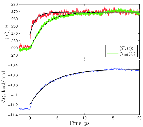
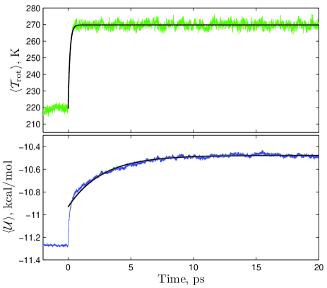
Figure 1: (Color online) Relaxation dynamics with translational Langevin thermostat: γ=4.0𝛾4.0\gamma=4.0\,ps-1, Γ=0Γ0\Gamma=0. Thin lines show relaxation dynamics averaged over ten independent runs, thick lines (solid and dashed for translational and rotational temperatures, respectively) show the least squares fit to formula (42). The estimated values of the relaxation times are τ𝒯tr=0.2subscript𝜏subscript𝒯tr0.2\tau_{\mathcal{T}_{\mathrm{tr}}}=0.2\,ps, τ𝒯rot=1.9subscript𝜏subscript𝒯rot1.9\tau_{\mathcal{T}_{\mathrm{rot}}}=1.9\,ps, and τ𝒰=3.6subscript𝜏𝒰3.6\tau_{\mathcal{U}}=3.6\,ps.

To illustrate the response of the system to the instantaneous temperature change, we show in Fig. 1 the result of applying the Langevin thermostat only to the translational degrees of freedom, i.e. Γ=0Γ0\Gamma=0 in (14)-(15). As expected, the translational kinetic temperature quickly relaxes to the new temperature, while the rotational kinetic temperature and potential energy lag behind. To estimate the relaxation rates of the measured quantities, we use the least squares fit of the exponential function (42) to the average measured quantity A(t)delimited-⟨⟩𝐴𝑡\langle A(t)\rangle.

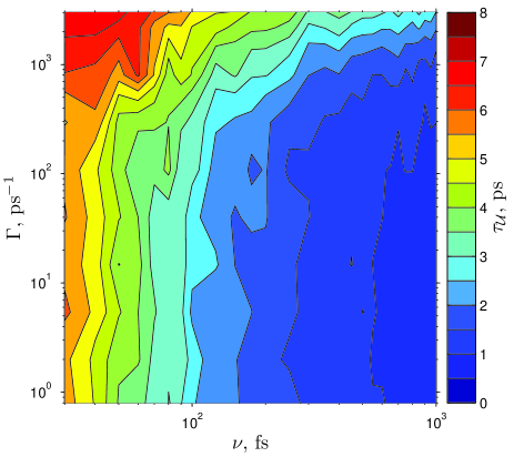
In all the simulations we performed, the potential energy relaxation time is larger than that for either of the kinetic temperatures. Therefore, we determine the relaxation time of the system to the new equilibrium state based on the value of τ𝒰subscript𝜏𝒰\tau_{\mathcal{U}}.

Refer to caption
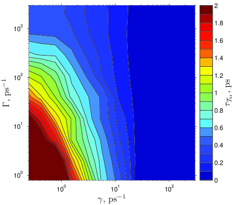
Figure 2: (Color online) Translational temperature relaxation time for the Langevin thermostat (14)-(15) as a function of the thermostat parameters γ𝛾\gamma and ΓΓ\Gamma.
Refer to caption
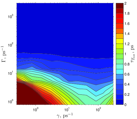
Figure 3: (Color online) Rotational temperature relaxation time for the Langevin thermostat (14)-(15) as a function of the thermostat parameters γ𝛾\gamma and ΓΓ\Gamma.
Refer to caption
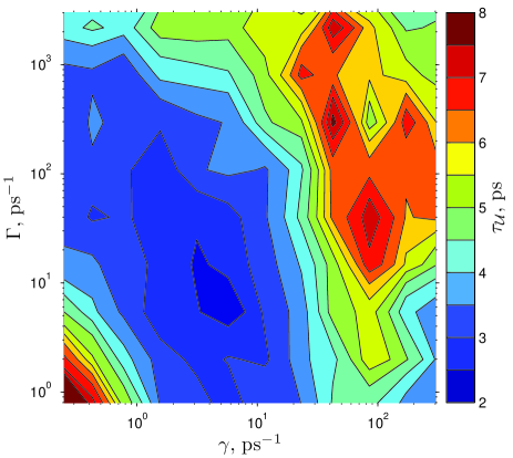
Figure 4: (Color online) Potential energy relaxation time for the Langevin thermostat (14)-(15) as a function of the thermostat parameters γ𝛾\gamma and ΓΓ\Gamma.

Varying the value of the translational Langevin parameter γ𝛾\gamma, we observe that relaxation is slower for both small and large values of γ𝛾\gamma, with the fastest relaxation around γ=4.0𝛾4.0\gamma=4.0\,ps-1. The existence of an optimal value for the choice of the thermostat parameter is consistent with observations in Ref. Bus06, and can be understood in terms of the interaction of the system with the thermostat. For small values of γ𝛾\gamma, the relaxation of the system is slow due to the limited heat flux between the system and the thermostat. For large γ𝛾\gamma, even though the kinetic temperature relaxes very quickly, the relaxation of the configurational state of the system is apparently hindered by the disruptive influence of the random force on the Hamiltonian dynamics which is driving the system to the new equilibrium.
Refer to caption
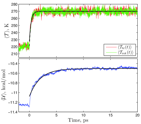
Figure 5: (Color online) Relaxation dynamics with ‘optimal’ choice of Langevin thermostat parameters: γ=4.0𝛾4.0\gamma=4.0\,ps-1, Γ=10.0Γ10.0\Gamma=10.0\,ps-1. Thin lines show relaxation dynamics averaged over ten independent runs, thick lines (solid and dashed for translational and rotational temperatures, respectively) show the least squares fit to formula (42). The estimated values of the relaxation times are τ𝒯tr=0.28subscript𝜏subscript𝒯tr0.28\tau_{\mathcal{T}_{\mathrm{tr}}}=0.28\,ps, τ𝒯rot=0.26subscript𝜏subscript𝒯rot0.26\tau_{\mathcal{T}_{\mathrm{rot}}}=0.26\,ps, and τ𝒰=2.0subscript𝜏𝒰2.0\tau_{\mathcal{U}}=2.0\,ps.

IV.1 Langevin Thermostats

Next, we investigate the dependence of the system relaxation time τ𝒰subscript𝜏𝒰\tau_{\mathcal{U}} on both γ𝛾\gamma and ΓΓ\Gamma in (14)-(15). In order to minimize the influence of the numerical discretization error, we use a relatively small time step of 0.20.20.2 fs. With such a small time step, the difference between Langevin A and Langevin B is negligible compared to the sampling error. To produce the results reported below, we use Langevin A. We evaluate τ𝒰subscript𝜏𝒰\tau_{\mathcal{U}} on a logarithmic grid of γ𝛾\gamma and ΓΓ\Gamma values using five independent runs at each point. The results are shown in Figs. 2, 3, and 4. As expected, the relaxation speed of translational and rotational temperatures uniformly increases with increasing values of γ𝛾\gamma and ΓΓ\Gamma, respectively. At the same time, the relaxation speed of the potential energy exhibits nonuniform dependence on the thermostat parameters. As can be seen in Fig. 4, the fastest relaxation of the system is achieved when the Langevin thermostat is applied to both translational and rotational degrees of freedom, with γ=28𝛾28\gamma=2-8 ps-1 and Γ=340Γ340\Gamma=3-40 ps-1. The relaxation dynamics of the system with ‘optimal’ choice of Langevin thermostat parameters is demonstrated in Fig. 5. In this case τ𝒯tr=0.28subscript𝜏subscript𝒯tr0.28\tau_{\mathcal{T}_{\mathrm{tr}}}=0.28\,ps, τ𝒯rot=0.26subscript𝜏subscript𝒯rot0.26\tau_{\mathcal{T}_{\mathrm{rot}}}=0.26\,ps, and τ𝒰=2.0subscript𝜏𝒰2.0\tau_{\mathcal{U}}=2.0\,ps, which shows that the system relaxation is almost twice as fast as when the Langevin thermostat is applied only to translational degrees of freedom. Note that the results shown in Fig. 4 for γ𝛾\gamma larger than about 100100100\,ps-1 or ΓΓ\Gamma larger than about 100010001000\,ps-1 are not reliable due to excessive coupling of the system to the thermostat, which disrupts the Hamiltonian flow of the system. In this case, the relaxation dynamics is poorly represented by the exponential function (42) and thus the fits produce misleading values for the system relaxation time.
Refer to caption
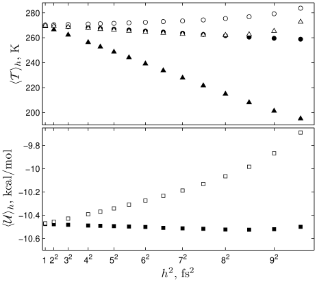
Figure 6: Dependence of the approximated average properties of a system of 2000 TIP4P water molecules on the integration time step hh for Langevin A and B. The system is equilibrated with the thermostat parameters γ=4.0𝛾4.0\gamma=4.0 ps-1, Γ=10.0Γ10.0\Gamma=10.0 ps-1, and T=270𝑇270T=270 K. The quantities 𝒯trhsubscriptdelimited-⟨⟩subscript𝒯tr\langle\mathcal{T}_{\mathrm{tr}}\rangle_{h}, 𝒯rothsubscriptdelimited-⟨⟩subscript𝒯rot\langle\mathcal{T}_{\mathrm{rot}}\rangle_{h}, and 𝒰hsubscriptdelimited-⟨⟩𝒰\langle\mathcal{U}\rangle_{h} are denoted by circles, triangles, and squares, respectively. Solid and open symbols refer to Langevin A and B, respectively.

Now we look at performance of the numerical integrators proposed in Section III.1 for the Langevin thermostat (14)-(15). Since both Langevin A and B are second-order methods, the calculated average quantities for simulations with step size hh should have the formTAT90 ; MT6

Ah=A0+CAh2+O(h3),subscriptdelimited-⟨⟩𝐴subscriptdelimited-⟨⟩𝐴0subscript𝐶𝐴superscript2𝑂superscript3\langle A\rangle_{h}=\langle A\rangle_{0}+C_{A}h^{2}+O(h^{3})\,, (46)

where Ahsubscriptdelimited-⟨⟩𝐴\langle A\rangle_{h} denotes the average value of dynamical quantity A(t)𝐴𝑡A(t) calculated over a numerical trajectory with time step hh. The dependence of 𝒯trhsubscriptdelimited-⟨⟩subscript𝒯tr\langle\mathcal{T}_{\mathrm{tr}}\rangle_{h}, 𝒯rothsubscriptdelimited-⟨⟩subscript𝒯rot\langle\mathcal{T}_{\mathrm{rot}}\rangle_{h}, and 𝒰hsubscriptdelimited-⟨⟩𝒰\langle\mathcal{U}\rangle_{h} on hh for both Langevin A and B is illustrated in Fig. 6. It appears that Langevin A has larger discretization error for the rotational temperature and smaller error for the potential energy than Langevin B. The linear dependence of the measured quantities on h2superscript2h^{2} is maintained up to a relatively large time step of about h=77h=7\,fs. The values of the slopes CAsubscript𝐶𝐴C_{A} are listed in Table 1. Both methods become unstable at about h=1010h=10\,fs.

Table 1: Values of the coefficients CAsubscript𝐶𝐴C_{A} in the discretization errors (46) for the measured quantities with Langevin A and B. The system’s parameters are as in Fig. 6.
Langevin A Langevin B
C𝒯trsubscript𝐶subscript𝒯trC_{\mathcal{T}_{\mathrm{tr}}} , K/fs2 0.130.13-0.13 0.060.060.06
C𝒯rotsubscript𝐶subscript𝒯rotC_{\mathcal{T}_{\mathrm{rot}}} , K/fs2 0.850.85-0.85 0.140.14-0.14
C𝒰subscript𝐶𝒰C_{\mathcal{U}} , kcal/mol/fs2 0.00070.0007-0.0007 0.00560.00560.0056
Refer to caption
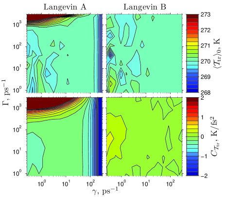
Figure 7: (Color online) Dependence of 𝒯tr0subscriptdelimited-⟨⟩subscript𝒯tr0\langle\mathcal{T}_{\mathrm{tr}}\rangle_{0} and C𝒯trsubscript𝐶subscript𝒯trC_{\mathcal{T}_{\mathrm{tr}}} on γ𝛾\gamma and ΓΓ\Gamma for Langevin A and B thermostats.
Refer to caption
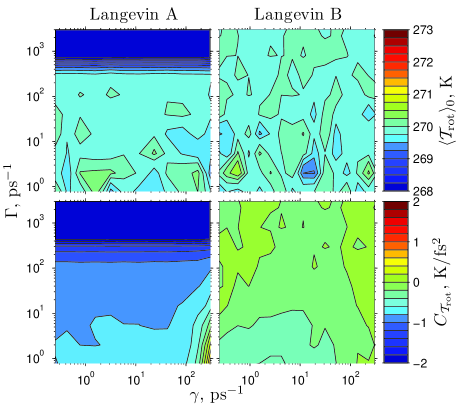
Figure 8: (Color online) Dependence of 𝒯rot0subscriptdelimited-⟨⟩subscript𝒯rot0\langle\mathcal{T}_{\mathrm{rot}}\rangle_{0} and C𝒯rotsubscript𝐶subscript𝒯rotC_{\mathcal{T}_{\mathrm{rot}}} on γ𝛾\gamma and ΓΓ\Gamma for Langevin A and B thermostats.
Refer to caption
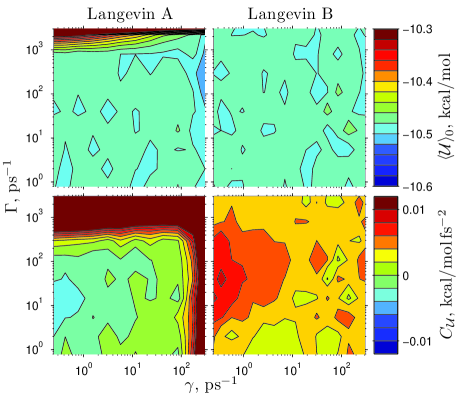
Figure 9: (Color online) Dependence of 𝒰0subscriptdelimited-⟨⟩𝒰0\langle\mathcal{U}\rangle_{0} and C𝒰subscript𝐶𝒰C_{\mathcal{U}} on γ𝛾\gamma and ΓΓ\Gamma for Langevin A and B thermostats.

We have investigated the dependence of A0subscriptdelimited-⟨⟩𝐴0\langle A\rangle_{0} and CAsubscript𝐶𝐴C_{A} on the thermostat parameters γ𝛾\gamma and ΓΓ\Gamma, by running simulations with time steps h=22h=2\,fs and 333\,fs and estimating these quantities from the straight line fit with respect to h2superscript2h^{2}. We consider the fit to be justified if the higher order terms in (46) are small, i.e., when the quantities 𝒯tr0subscriptdelimited-⟨⟩subscript𝒯tr0\langle\mathcal{T}_{\mathrm{tr}}\rangle_{0} and 𝒯rot0subscriptdelimited-⟨⟩subscript𝒯rot0\langle\mathcal{T}_{\mathrm{rot}}\rangle_{0} determined from (46) are equal to the thermostat temperature parameter T=270𝑇270T=270\,K. In Fig. 7 we show results for the translational temperature measurements in simulations with Langevin A and B. As expected, 𝒯tr0subscriptdelimited-⟨⟩subscript𝒯tr0\langle\mathcal{T}_{\mathrm{tr}}\rangle_{0} converges to 270270270\,K. We note in passing that smaller statistical errors are observed at larger values of γ𝛾\gamma. The behavior of C𝒯trsubscript𝐶subscript𝒯trC_{\mathcal{T}_{\mathrm{tr}}} for Langevin A exhibits a plateau for small and moderate values of γ𝛾\gamma and ΓΓ\Gamma and then changes rapidly at values that are ‘too large’ for this system. By contrast, the translational temperature discretization error of Langevin B thermostat exhibits consistent behavior for all values of γ𝛾\gamma and ΓΓ\Gamma. Similar differences between Langevin A and B can be seen in the measurements of rotational temperature and potential energy shown in Figs. 8 and 9, respectively. As can be seen from the plot of 𝒯rot0subscriptdelimited-⟨⟩subscript𝒯rot0\langle\mathcal{T}_{\mathrm{rot}}\rangle_{0} in Fig. 8, the straight line fit also breaks down at large ΓΓ\Gamma values in Langevin A.

IV.2 Gradient-Langevin thermostat

Here we describe numerical experiments with the gradient-Langevin thermostat (17)-(18) introduced in Section II.2. Since the gradient system for the translational motion does not include linear momenta 𝐏𝐏\mathbf{P}, the translational kinetic temperature 𝒯trsubscript𝒯tr\mathcal{T}_{\mathrm{tr}} is not available for measurement in this case. Therefore, in our numerical experiments we measure the rotational temperature 𝒯rotsubscript𝒯rot\mathcal{T}_{\mathrm{rot}} and potential energy per particle 𝒰𝒰\mathcal{U} as defined by (44) and (45), respectively.

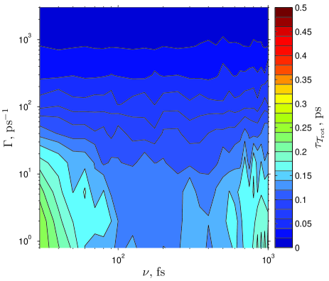
For the particular system studied here, the gradient-Langevin numerical scheme (34), (25) from Section III.2 becomes unstable when the product hν𝜈h\nu is larger than about 200200200\,fs2. Therefore, with the step size of h=0.20.2h=0.2\,fs used in our simulations, we can study the properties of the gradient-Langevin scheme with ν𝜈\nu up to about 100010001000\,fs.

Refer to caption
Figure 10: (Color online) Rotational temperature relaxation time for the gradient-Langevin thermostat (17)-(18) as a function of the thermostat parameters ν𝜈\nu and ΓΓ\Gamma.
Refer to caption
Figure 11: (Color online) Potential energy relaxation time for the gradient-Langevin thermostat (17)-(18) as a function of the thermostat parameters ν𝜈\nu and ΓΓ\Gamma.
Refer to caption
Figure 12: (Color online) Relaxation dynamics with gradient-Langevin thermostat: ν=100𝜈100\nu=100\,fs, Γ=0Γ0\Gamma=0. Thin lines show relaxation dynamics averaged over seven independent runs, thick lines show the least squares fit to formula (42).

We conducted the relaxation experiment, where we monitored 𝒯rot(t)delimited-⟨⟩subscript𝒯rot𝑡\langle\mathcal{T}_{\mathrm{rot}}(t)\rangle and 𝒰(t)delimited-⟨⟩𝒰𝑡\langle\mathcal{U}(t)\rangle while the thermostat temperature parameter was switched from 220 K to 270 K. The relaxation times τ𝒯rotsubscript𝜏subscript𝒯rot\tau_{\mathcal{T}_{\mathrm{rot}}} and τ𝒰subscript𝜏𝒰\tau_{\mathcal{U}} for these quantities were calculated for different values of ν𝜈\nu and ΓΓ\Gamma. The results are shown in Figs. 10 and 11. As expected, the relaxation time for rotational temperature decreases with increasing value of ΓΓ\Gamma. The somewhat surprising finding of this experiment is that, even for small values of ΓΓ\Gamma the relaxation time is much smaller here than in the case of Langevin thermostat (see Fig. 3). As an illustration, we show the relaxation experiment for ν=100𝜈100\nu=100\,fs and Γ=0Γ0\Gamma=0 in Fig. 12. The estimated relaxation time for rotational temperature, τ𝒯rot=0.14subscript𝜏subscript𝒯rot0.14\tau_{\mathcal{T}_{\mathrm{rot}}}=0.14\,ps, is much smaller then the corresponding quantity for the Langevin thermostat, even though the relaxation time for the potential energy, τ𝒰=2.7subscript𝜏𝒰2.7\tau_{\mathcal{U}}=2.7\,ps, is similar. This indicates a very efficient heat transfer between the gradient dynamics of the translational motion and the rotational motion.

The dependence of τ𝒰subscript𝜏𝒰\tau_{\mathcal{U}} on the thermostat parameters for the gradient-Langevin system shown in Fig. 11 is markedly different than for the Langevin system. In particular, the relaxation time decreases with increasing ν𝜈\nu without reaching a minimum value within the range of ν𝜈\nu values explored. At the same time, there is little dependence on ΓΓ\Gamma, except for very large ΓΓ\Gamma where, similar to the Langevin system, the measurements of the relaxation time are not reliable. Also, note that the relaxation times are much smaller, reaching as low as 0.70.70.7\,ps for ν=1000𝜈1000\nu=1000\,fs, compared to the minimum value of about 2.02.02.0\,ps for the Langevin system.

Of course, the direct comparison between the relaxation speeds of gradient-Langevin and Langevin dynamics has to be taken with caution, since, as we mentioned in Section II.2, the gradient dynamics does not have a natural evolution time. In particular, the mass of the molecule m𝑚m does not have a specific meaning in the gradient system, since it can be rescaled to any value together with hh and ν𝜈\nu (see (17)). Computationally, the relaxation speed depends on the time step hh and, while with ν=1000𝜈1000\nu=1000\,fs the gradient Langevin scheme becomes unstable for hh larger than 0.20.20.2 fs, the Langevin scheme remains stable up to about h=1010h=10\,fs for the optimal values of γ=4.0𝛾4.0\gamma=4.0\,ps-1 and Γ=10Γ10\Gamma=10\,ps-1.

Refer to caption
Figure 13: Dependence of the approximated average properties of a system of 2000 TIP4P water molecules on the integration time step hh for the gradient-Langevin numerical method. The system is equilibrated with the thermostat parameters ν=200𝜈200\nu=200\,fs, Γ=5.0Γ5.0\Gamma=5.0\,ps-1, and T=270𝑇270T=270\,K. The quantities 𝒯rothsubscriptdelimited-⟨⟩subscript𝒯rot\langle\mathcal{T}_{\mathrm{rot}}\rangle_{h}, and 𝒰hsubscriptdelimited-⟨⟩𝒰\langle\mathcal{U}\rangle_{h} are denoted by circles and squares, respectively. Error bars reflect 95% confidence intervals in the obtained results estimated from block averages.

The dependence of discretization error in measured quantities on hh for the gradient-Langevin scheme is shown in Fig. 13. As in the case of Langevin A and B, we clearly see the linear dependence of 𝒯rothsubscriptdelimited-⟨⟩subscript𝒯rot\langle\mathcal{T}_{\mathrm{rot}}\rangle_{h}, and 𝒰hsubscriptdelimited-⟨⟩𝒰\langle\mathcal{U}\rangle_{h} on h2superscript2h^{2}. The estimated slopes in (46) are C𝒯rot=0.38subscript𝐶subscript𝒯rot0.38C_{\mathcal{T}_{\mathrm{rot}}}=-0.38\,K/fs2 and C𝒰=0.029subscript𝐶𝒰0.029C_{\mathcal{U}}=-0.029\,kcal/mol/fs2. Unfortunately, for this value of ν𝜈\nu the gradient-Langevin numerical integrator becomes unstable for h>11h>1\,fs, which is rather small, given that the Langevin A and B integrator are stable for hh up to about 10 fs. Still, given the observed efficient heat transfer from the gradient subsystem for translational dynamics to the rotational dynamics (see Fig. 12 and related discussion), it might be of interest to construct numerical methods for the gradient-Langevin system (17)-(18) with better stability properties than those of (34), (25); this has not been considered in this paper.

V Summary

The new stochastic thermostats presented in this paper are appropriate for quaternion-based rigid body models. They are written in the form of Langevin equations and gradient-Langevin system (gradient subsystem for the translational degrees of freedom and Langevin subsystem for the rotational degrees of freedom). The obtained stochastic systems preserve the unit length of the rotational coordinates in the quaternion representation of the rigid-body dynamics. The thermostats allow to couple both translational and rotational degrees of freedom to the “heat bath”. As it is shown in the numerical tests with the TIP4P rigid model of water, the Langevin thermostat relaxes to an equilibrium faster when not only translational degrees of freedom but also rotational ones are thermostated. It turns out that there is an optimal range of the strength of coupling to the “heat bath”. In contrast, the gradient-Langevin thermostat has a monotone dependence of relaxation time on the thermostat parameters. In the case of the Langevin thermostat, two quasi-symplectic second-order (in the weak sense) integrators are constructed and compared in the numerical tests. For the gradient-Langevin thermostat, a Runge-Kutta second-order method is proposed. All the methods preserve the unit length of the rotational coordinates. The numerical experiments demonstrate the efficiency of the proposed thermostating technique.

Relaxation times for the gradient-Langevin thermostat are smaller than for the Langevin thermostat. However, the numerical methods proposed for the Langevin system have better stability properties than the scheme used for numerical integration of the gradient-Langevin system. In our experimental study, the use of the Langevin thermostat together with the quasi-symplectic integrators was computationally significantly more efficient than thermostating via the gradient-Langevin system and the numerical scheme for it.

Acknowledgements.
The work of RLD and RH was supported by the EPSRC research grant GR/T27105/01 which is gratefully acknowledged. One of the authors (RLD) did part of the work during his study leave granted by the University of Leicester. The computations were performed on the University of Leicester Mathematical Modelling Centre s cluster, which was purchased through the EPSRC strategic equipment initiative.

References

  • (1) Hünenberger, P.H., Thermostat algorithms for molecular dynamics simulations, Adv. Polym. Sci., 173 (2005), 105–149.
  • (2) Miller III, T.F., Eleftheriou, M., Pattnaik, P., Ndirango, A., Newns, D., Matyna, G.J., Symplectic quaternion scheme for biophysical molecular dynamics, J. Chem. Phys., 116 (2002), 8649–8659.
  • (3) Leimkuhler, B., Reich, S., Simulating Hamiltonian Dynamics, Cambridge Univ. Press, 2005.
  • (4) Vanden-Eijnden, E., Ciccotti, G., Second-order integrators for Langevin equations with holonomic constraints, Chem. Phys. Lett., 429 (2006), 310–316.
  • (5) Sun, X., Lin, T., Gezelter, J. D., Langevin dynamics for rigid bodies of arbitrary shape, J. Chem. Phys., 128 (2008), 234107.
  • (6) Izaguirre, J.A., Catarello, D.P., Wozniak, J.M., Skeel, R.D. Langevin stabilization of molecular dynamics, J. Chem. Phys., 114 (2001), 2090–2098.
  • (7) Hasminskii, R.Z., Stochastic Stability of Differential Equations, Sijthoff & Noordhoff, 1980.
  • (8) Mattingly, J.C., Stuart, A.M., Higham, D.J., Ergodicity for SDEs and approximations: locally Lipschitz vector fields and degenerate noise, Stoch. Proc. Appl., 101 (2002), 185–232.
  • (9) Milstein, G.N., Repin, Yu.M., Tretyakov, M.V., Symplectic integration of Hamiltonian systems with additive noise, SIAM J. Numer. Anal., 39 (2002), 2066–2088.
  • (10) Milstein, G.N., Tretyakov, M.V., Quasi-symplectic methods for Langevin-type equations, IMA J. Numer. Anal., 23 (2003), 593–626.
  • (11) Milstein, G.N., Tretyakov, M.V., Stochastic Numerics for Mathematical Physics, Springer, 2004.
  • (12) Milstein, G.N., Tretyakov, M.V., Computing ergodic limits for Langevin equations, Physica D, 229 (2007), 81–95.
  • (13) Nelson, E., Dynamical Theories of Brownian Motion, Princeton Univ. Press, 1967.
  • (14) Skeel, R., Integration schemes for molecular dynamics and related applications, In: “Graduate Student’s Guide to Numerical Analysis’98” edited by M. Ainsworth, J. Levesley, M. Marletta, Springer, 1999, 118–176.
  • (15) Bussi, G., Parrinello, M., Accurate sampling using Langevin dynamics, Phys. Rev. E 75 (2007), 056707.
  • (16) Soize, C., The Fokker-Planck Equation for Stochastic Dynamical Systems and its Explicit Steady State Solutions, World Scientific, 1994.
  • (17) Talay, D., Second-order discretization schemes for stochastic differential systems for the computation of the invariant law, Stoch. Stoch. Rep., 29 (1990), 13–36.
  • (18) Talay, D., Stochastic Hamiltonian systems: exponential convergence to the invariant measure, and discretization by the implicit Euler scheme, Markov Proc. Relat. Fields, 8 (2002), 163–198.
  • (19) Jorgensen, W.L., Chandrasekhar, J., Madura, J., Impey, R.W., Klein, M.L., Comparison of simple potential functions for simulating liquid water, J. Chem. Phys., 79 (1983), 926–935.
  • (20) Handel, R., Davidchack, R.L., Anwar, J., Brukhno, A., Direct calculation of solid-liquid interfacial free energy for molecular systems: TIP4P ice-water interface, Phys. Rev. Lett., 100 (2008), 036104.
  • (21) Talay, D., Tubaro, L., Expansion of the global error for numerical schemes solving stochastic differential equations, Stoch. Anal. Appl., 8 (1990), 483–509.