Ergodic properties of boundary actions and Nielsen–Schreier theory

Abstract.

We study the basic ergodic properties (ergodicity and conservativity) of the action of an arbitrary subgroup $H$ of a free group $F$ on the boundary $\partial F$ with respect to the uniform measure. Our approach is geometrical and combinatorial, and it is based on choosing a system of Nielsen–Schreier generators in $H$ associated with a geodesic spanning tree in the Schreier graph $X=H\backslash F$. We give several (mod 0) equivalent descriptions of the Hopf decomposition of the boundary into the conservative and the dissipative parts. Further we relate conservativity and dissipativity of the action with the growth of the Schreier graph $X$ and of the subgroup $H$ ($\equiv$ cogrowth of $X$), respectively. We also construct numerous examples illustrating connections between various relevant notions.

Introduction

In 1921 Jacob Nielsen [Nie21] proved that any finitely generated subgroup of a free group is itself a free group. His proof was based on a rewriting procedure which allows one to reduce an arbitrary finite system of elements of a free group to a system of free generators. Since then Nielsen’s method has become one of the main tools in the combinatorial group theory [MKS76, LS01]. It is used in the study of the group of automorphisms of a free group, for solving equations in free groups and in numerous other applications. Its scope is by no means restricted to free groups and extends to the combinatorial group theory at large, $K$-theory and topology.

In 1927 Nielsen’s result was extended by Otto Schreier [Sch27] to arbitrary subgroups in another seminal work (where, in particular, what is currently known as Schreier graphs was introduced). Under the name of the Nielsen–Schreier theorem it is now one of the bases of the theory of infinite groups. Schreier’s method is at first glance quite different from Nielsen’s and uses families of coset representatives (transversals). That Nielsen and Schreier actually arrived at essentially the same generating systems became clear much later and was proved in [HR48, KS58].

In this work we show that the Nielsen–Schreier theory is useful in the ergodic theory, and our main result is its application to the study of the ergodic properties of the boundary action of arbitrary subgroups of a finitely generated free group. On the other hand, our point of view “from infinity” (based on using dynamical invariants of the boundary action) sheds new light on geometry of Schreier graphs and associated subgroups.

The boundary theory occupies an important place in various mathematical fields: geometric group theory, rigidity theory, theory of Kleinian groups, potential analysis, Markov chains, to name just a few. The free group is one of the central objects in the study of boundaries of groups. Its simple combinatorial structure makes of it a convenient test-case which contributes to the understanding of general concepts, both in the group-theoretic (as the free group is the universal object in the category of discrete groups) and geometric (as its Cayley graph, the homogeneous tree, is a discrete analogue of the constant curvature hyperbolic space) frameworks.

There exist many different boundaries of a group corresponding to various compactifications: the space of ends, the Martin boundary, the visual boundary, the Busemann boundary, the Floyd boundary, etc. There is also a measure-theoretical notion of the Poisson(–Furstenberg) boundary, which is the one especially important for the present study. In the case of the free group $F$ freely generated by a finite set $\mathcal{A}$, all these notions coincide, and the boundary $\partial F$ can be realized as the space ${\breve{\mathcal{A}}}_{r}^{\infty}$ of infinite freely reduced words in the alphabet ${\breve{\mathcal{A}}}=\mathcal{A}\cup\mathcal{A}^{-1}$. The action of the group on itself extends by continuity to a continuous action on $\partial F$.

The choice of the generating set $\mathcal{A}$ determines a natural uniform probability measure $\mathfrak{m}$ on $\partial F$ which is quasi-invariant under the action of $F$. This measure can also be interpreted in a number of other ways. Namely, as the measure of maximal entropy of the unilateral Markov shift in the space of infinite irreducible words, as a conformal density (Patterson measure), or as the hitting ($\equiv$ harmonic) measure of the simple random walk on the group. In the latter interpretation the measure space $(\partial F,\mathfrak{m})$ is actually isomorphic to the Poisson boundary of the random walk, and it is this interpretation that plays an important role in our work.

The main goal of the present paper is to study the basic ergodic properties, i.e., ergodicity and conservativity, of the action of an arbitrary subgroup $H\leq F$ on the boundary $\partial F$ with respect to the measure $\mathfrak{m}$. Our principal results are:

• An explicit combinatorial description of the Hopf decomposition of the boundary action in terms of what we call the Schreier limit set (Theorem 1.21 and Theorem 2.12);

• Identification of the conservative part of the Hopf decomposition with the horospheric limit set (Theorem 3.21);

• A sufficient condition of complete dissipativity of the boundary action (Theorem 4.2) and a necessary and sufficient condition of its conservativity (Theorem 4.12) in terms of the growth of the group $H$ ($\equiv$ the cogrowth of the associated Schreier graph $X$) and of $X$, respectively;

• Numerous new examples illustrating and clarifying the interrelations between various conditions (Section 3.G and Section 4.D).

On the other hand, we expect our approach to be useful for purely algebraic problems as well. For instance, our analysis of the ergodic properties of the boundary action allows us to give a conceptual proof of an old theorem of Karrass–Solitar on finitely generated subgroups of a free group (Remark 3.33).

Recall that an action of a countable group is called ergodic with respect to a quasi-invariant measure if it has no non-trivial invariant sets. Any action (on a Lebesgue space) admits a unique ergodic decomposition into its ergodic components. An action is called conservative if it admits no non-trivial wandering set (i.e, such that its translations are pairwise disjoint). There is always a maximal wandering set, and the union of its translations is called the dissipative part of the action. Any action admits the so-called Hopf decomposition into the conservative and dissipative parts. These parts can also be described as the unions of all the purely non-atomic, and, respectively, of all the atomic ergodic components. It is important to keep in mind that the Hopf decomposition (as well as other measure theoretic notions) is defined (mod 0), i.e., up to measure $0$ subsets.

It is pretty straightforward to see that ergodicity of the boundary action is equivalent to the Liouville property of the simple random walk on the Schreier graph $X$ (i.e., to the absence of non-constant bounded harmonic functions on $X$), see Section 3.E. On the other hand, as was shown by Kaimanovich [Kai95], the boundary action of a non-trivial normal subgroup is always conservative. In particular, if $G=F/H$ is any non-Liouville (for example, non-amenable) group, then the action of the normal subgroup $H$ on $(\partial F,\mathfrak{m})$ is conservative without being ergodic. The only other previously known example of the Hopf decomposition of a boundary action was the one of completely dissipative $\mathbb{Z}$-actions [Kai95].

The starting point of our approach is the Schreier graph structure on the quotient homogeneous space $X=H\backslash F$. To quote [Sti93, Section 2.2.6], Schreier’s method “begs to be interpreted in terms of spanning trees” in the Schreier graph. Indeed, there is a one-to-one correspondence between Schreier generating systems for the subgroup $H$ and spanning trees in $X$ rooted at the origin $o=H$, which we remind in Section 1.A and Section 1.B. This correspondence consists in assigning the associated cycle in $X$ to any edge removed when passing to the spanning tree (Theorem 1.8).

By interpreting points of the boundary $\partial F$ as infinite paths without backtracking issued from the origin $o=H$ in the Schreier graph $X$, we define two subsets of $\partial F$: the Schreier limit set $\Omega$ and the Schreier fundamental domain $\Delta$ (Definition 1.15). The set $\Omega$ corresponds to the paths which pass infinitely many times through $\mathsf{Edges}(X)\setminus\mathsf{Edges}(T)$ and is homeomorphic to the set $\partial H$ of infinite irreducible words in the alphabet $\breve{\mathcal{S}}=S\sqcup S^{-1}$, whereas the set $\Delta$ corresponds to the rays issued from the origin in the tree $T$, and is homeomorphic to the boundary $\partial T$ of $T$. These sets give rise to a decomposition $\partial F=\left(\bigsqcup_{h\in H}h\Delta\right)\sqcup\Omega$ (Theorem 1.21).

However, in order to study this decomposition further we have to impose an additional condition on the Schreier generating system by requiring it to be minimal, which means that the corresponding spanning tree $T$ is geodesic (the class of minimal Schreier systems coincides with the class of Nielsen generating systems, see Section 1.E and the references therein). Under this assumption we prove that the above decomposition, indeed, coincides (mod 0) with the Hopf decomposition of the boundary action (Theorem 2.12).

The topological counterpart of the Hopf decomposition of the boundary action is the decomposition of the boundary $\partial F$ into a union of the closed $H$-invariant limit set $\Lambda=\Lambda_{H}$ (the closure of $H$ in the compactification $\widehat{F}=F\cup\partial F$) and its complement $\Lambda^{c}$. According to a general result (valid for all Gromov hyperbolic spaces), the restriction of the $H$-action to $\Lambda$ is minimal (any orbit is dense), whereas its restriction to $\Lambda^{c}$ is properly discontinuous (no orbit has accumulation points). The decomposition $\partial F=\Lambda\sqcup\Lambda^{c}$ corresponds to the decomposition of the Schreier graph $X$ into a union of its core $X_{*}$ and the collection of hanging branches (Theorem 3.8; see Section 3.A for the definitions). In particular, $\Lambda=\partial F$ if and only if $X$ has no hanging branches.

The Schreier limit set $\Omega$ is contained in the full limit set $\Lambda$, which corresponds to the fact that proper discontinuity of the boundary action on $\Lambda^{c}$ implies its complete dissipativity with respect to any quasi-invariant measure (in particular, the uniform measure $\mathfrak{m}$). Geometrically, any hanging branch in $X$ gives rise to a non-trivial wandering set in $\Lambda^{c}$. However, the action on $\Lambda$ may also have a non-trivial dissipative part, or even be completely dissipative. For instance, it may so happen that the Schreier graph $X$ has no hanging branches at all (i.e., $\Lambda=\partial F$), but nonetheless the boundary action is completely dissipative (Example 4.19).

We introduce the small (resp., big) horospheric limit set $\Lambda^{horS}=\Lambda^{horS}_{H}$ (resp., $\Lambda^{horB}=\Lambda^{horB}_{H}$) of the subgroup $H$ as the set of all the points $\omega\in\Lambda$ such that any (resp., a certain) horoball centered at $\omega$ contains infinitely many points from $H$, and show that the Schreier limit set $\Omega$ is sandwiched between $\Lambda^{horS}$ and $\Lambda^{horB}$, but coincides with them (mod 0) with respect to the measure $\mathfrak{m}$ (Theorem 3.20 and Theorem 3.21). We also establish certain other inclusions and show by appropriate examples that all of them are strict (Section 3.G).

If the subgroup $H$ is finitely generated (i.e, if the core $X_{*}$ is finite), then the Hopf alternative between conservativity and complete dissipativity holds: either the Schreier graph $X$ is finite and the boundary action of $H$ is ergodic (therefore, conservative), or $X$ is infinite and the boundary action is completely dissipative (Theorem 3.30). However, for infinitely generated subgroups the relationship between the ergodic properties of the boundary action and the geometry of the Schreier graph $X$ is much more complicated (as illustrated by numerous examples in Section 4.D).

We prove that if the exponential growth rate of $H$ ($\equiv$ the cogrowth of $X$) satisfies the inequality $v_{H}<\sqrt{2m-1}$, where $m$ is the number of generators of $F$ (i.e., if $v_{H}<\sqrt{v_{F}}$), then the boundary action of $H$ is completely dissipative (Theorem 4.2). On the other hand, we show (Theorem 4.12) that the boundary action of $H$ is conservative if and only if $\lim_{n}|S_{X}^{n}|/|S_{F}^{n}|=0$, where $S_{X}^{n}$ (resp., $S_{F}^{n}$) is the radius $n$ sphere in $X$ (resp., $F$) centered at the origin $o$ (resp., at the identity $e$). In particular, if the exponential growth rate $v_{X}$ of the Schreier graph $X$ satisfies the inequality $v_{X}<2m-1$, then the boundary action is conservative (Corollary 4.14).

Markov chains (not only the aforementioned simple random walks, but also the other chains described in Section 5) play an important role in understanding the ergodic properties of the boundary action. Another measure-theoretical tool which we use in this paper is the relationship of the boundary action with two other natural actions of the subgroup $H$ (see Section 3.F for references and more details).

The first one is the action on the square $\partial^{2}F$ of the boundary $\partial F$ endowed with the square of the uniform measure $\mathfrak{m}$. The ergodic properties of this action are the same as for the (discrete) geodesic flow on the Schreier graph $X$ and are described by the classical Hopf alternative (Theorem 3.35): the action of $H$ on $(\partial^{2}F,\mathfrak{m}^{2})$ is either ergodic (therefore, conservative) or completely dissipative. Moreover, ergodicity of this action is equivalent to divergence of the Poincaré series $\sum_{h\in H}(2m-1)^{-|h|}$. Note that the ergodic behaviour of the action on $\partial F$ is much more complicated than of that on $\partial^{2}F$: for instance, the Hopf alternative for the former, generally speaking, holds only in the finitely generated case. It is interesting that one of our descriptions of the Hopf decomposition of the action on $\partial F$ deals with a series similar to the Poincaré series arising for the action on $\partial^{2}F$. However, once again, it is more complicated as it involves the Busemann functions rather than plain distances (see Theorem 2.12 and Theorem 3.21).

The second auxiliary action is the action of the group $H$ on the space of horospheres in $F$, i.e., the $\mathbb{Z}$-extension of the action on $\partial F$ determined by the Busemann cocycle. Geometrically, this action corresponds to what could be called (by analogy with Fuchsian groups) “horocycle flow” on the Schreier graph. We use the fact that (unlike for the action on $\partial^{2}F$) the ergodic properties of this action are precisely the same as for the original action on $\partial F$ (Theorem 3.38).

It is a commonplace that the homogeneous tree is a “rough sketch” of the hyperbolic plane. Both these spaces are Gromov hyperbolic (even CAT($-1$)), and their isometry groups are “large enough” (so that the rotations around any reference point inside act transitively on the hyperbolic boundary). The subgroups of the free group $F$, which are the object of our consideration, are just the torsion free discrete groups of isometries of the Cayley tree of $F$. Thus, the question about analogous results for discrete isometry groups in the hyperbolic setup — be it for the usual hyperbolic plane (Fuchsian groups), higher dimensional simply connected spaces of constant negative curvature (Kleinian groups), arbitrary non-compact rank 1 symmetric spaces, general CAT($-1$) or Gromov hyperbolic spaces, even for spaces which are hyperbolic in a weaker form — cannot fail to be asked.

The work on the present article prompted the second author to show that the identification of the conservative part of the boundary action with the big horospheric limit set $\Lambda^{horB}$ is actually valid in the full generality of a discrete group of isometries of an arbitrary Gromov hyperbolic space endowed with a quasi-conformal boundary measure [Kai10] (see the references therein for a list of earlier particular cases of this result). The proof uses the fact that, by definition, the logarithms of the Radon–Nikodym derivatives of such a measure are (almost) proportional to the Busemann cocycle, in combination with the description of the Hopf decomposition of an arbitrary action in terms of the orbitwise sums of the Radon–Nikodym derivatives (Theorem 2.2). However, this is the only situation in our paper when the cases of the free group and of the hyperbolic plane are specializations of a common general result. Even here we obtain, in terms of Nielsen–Schreier generators, a much more detailed information about the Hopf decomposition than in the general case (Theorem 3.21).

Two other occasions when our results have analogues for Fuchsian or Kleinian groups are Theorem 4.2 and Theorem 4.12 from Section 4 which give qualitative criteria of complete dissipativity and conservativity of the boundary action, respectively. Here common general results are unknown, and our methods are completely different from those used in the hyperbolic situation by Patterson [Pat77] and Matsuzaki [Mat05] in the first case (see Remark 4.6) and by Sullivan [Sul81] in the second case (see Remark 4.16). Although the “hyperbolic” techniques most likely might be carried over to our situation as well, our approach is much more appropriate in the discrete case as it uses combinatorial tools not readily available in the continuous case. For instance, we obtain Theorem 4.12 as a corollary of Theorem 4.10 which gives an explicit formula for the measure of a certain canonical wandering set; a hyperbolic analogue of Theorem 4.10 is unknown.

Let us finally mention some open questions arising in connection with the present work. The most obvious one is to what extent our results can be carried over to other boundary measures. The first candidate would be the conformal (Patterson) measures which are singular with respect to the uniform measure $\mathfrak{m}$ in the case when the growth $v_{H}$ of $H$ is strictly smaller than the growth of the ambient group $F$. By a general result from [Kai10], in this case the conservative part can still be identified with the big horospheric limit set (see above), but we do not know to what extent the combinatorial machinery developed in the present paper can be adapted to this situation. Of course, one can also try to generalize our technique to the nearest relatives of free groups, i.e., to word hyperbolic groups, or even to general discrete groups of isometries of Gromov hyperbolic spaces.

In a different direction, it would be interesting to investigate the properties described in the present paper for random Schreier graphs determined by a probability measure invariant with respect to the “root moving” equivalence relation (in other words, a conjugation invariant probability measure on the space of subgroups of $F$, see [Ver10, AGV11]).

Finally, a more concrete question concerns existence of conservative boundary actions (with respect to the uniform measure) with $v_{H}=\sqrt{2m-1}$, cf. Theorem 4.2. The analogous question is also open for Fuchsian groups, see Remark 4.4 and Remark 4.6. For the free group this situation is especially intriguing because from the spectral point of view Schreier graphs with $v_{H}\leq\sqrt{2m-1}$ are precisely the infinite Ramanujan graphs (i.e., have the minimal possible spectral radius, see formula (4.1)). Our Theorem 4.2 implies, in the case when $v_{H}<\sqrt{2m-1}$, some properties conjectured to be true for all infinite Ramanujan graphs: absence of the Liouville property [BK10, Conjecture 1] and the fact that the random walk neighbourhood sampling along the graph converges to the regular tree [Abé10, Question 11].

1. Nielsen–Schreier theory and the boundary action

Let $F$ denote the free group freely generated by a finite set $\mathcal{A}$ with $|\mathcal{A}|=m\geq 2$, and let ${\breve{\mathcal{A}}}=\mathcal{A}\sqcup\mathcal{A}^{-1}$. The Cayley graph $\Gamma(F,{\breve{\mathcal{A}}})$ is a homogeneous tree of degree $|{\breve{\mathcal{A}}}|=2|\mathcal{A}|$.

We shall use the notation ${\breve{\mathcal{A}}}^{*}$ (resp., ${\breve{\mathcal{A}}}^{\infty}$) for the sets of all finite (resp., right infinite) words in the alphabet ${\breve{\mathcal{A}}}$. The length of a word $w$ is denoted by $|w|$. For the subsets of ${\breve{\mathcal{A}}}^{*}$ and ${\breve{\mathcal{A}}}^{\infty}$ consisting of freely reduced words we shall add the subscript $r$, so that there is a canonical map

(1.1) $$\sigma:F\to{\breve{\mathcal{A}}}^{*}_{r}$$

identifying $F$ and ${\breve{\mathcal{A}}}^{*}_{r}$.

Any subgroup $H\leq F$ of a free group $F$ is also free. It was proved by Nielsen [Nie21] (for finitely generated subgroup) and Schreier [Sch27] by giving two different constructions of free generating sets in $H$, see [MKS76] and the references therein. As it turned out, Nielsen’s generating systems are just a particular case of Schreier’s systems (see Theorem 1.24 below). We shall begin by recasting the original symbolic construction of Schreier (described in [MKS76, Section 2.3]) in terms of spanning trees in the Schreier graph $X\cong H\backslash F$ (cf. [Sti93, Section 2.2.6] and [KM02, Section 6]). Further we shall construct a decomposition of the boundary $\partial F$ naturally associated with such a spanning tree (Theorem 1.21), which is the main goal of this Section.

1.A. Spanning trees and Schreier transversals

Given a subgroup $H\leq F$, denote by $\Gamma(X,{\breve{\mathcal{A}}})$ the Schreier graph of the homogeneous space $X=H\backslash F$ with respect to ${\breve{\mathcal{A}}}$, i.e., two cosets $Hg_{1},Hg_{2}\in X$ are connected with an edge if and only if $g_{1}^{-1}g_{2}\in{\breve{\mathcal{A}}}$, in which case the oriented edge $[Hg_{1},Hg_{2}]$ is labelled with $g_{1}^{-1}g_{2}$. Notice that, unlike the Cayley graph, the Schreier graph may have multiple edges with the same endpoints (but different labels). The extreme example is $H=F$, when $X$ consists of just one vertex with $|\mathcal{A}|$ attached loops. In the sequel we shall always assume that $X$ is endowed with the Schreier graph structure.

The Schreier graph $X$ has a distinguished vertex $o=H$, it is connected, $|{\breve{\mathcal{A}}}|$-regular (loops attached to points $x\in X$ with $xg=g$ for certain $g\in{\breve{\mathcal{A}}}$ are also counted!), and the set of edge labels around each vertex is precisely ${\breve{\mathcal{A}}}$. Moreover, the labels assigned to two different orientations of any edge are mutually inverse. Conversely, any graph with the above properties is the Schreier graph associated with a subgroup of $F$.

Remark 1.2.

By a theorem of Gross any regular graph of even degree can be realized as the Schreier graph associated to a subgroup of a free group (i.e., its edges can be labelled in the aforementioned way). It is explained in [Lub95] for finite graphs; an inductive argument can be used to carry the proof over to infinite graphs (also see [dlH00]).

It will be convenient to use the following geometric interpretation of the set of irreducible words in the alphabet ${\breve{\mathcal{A}}}$:

Proposition 1.3.

The set ${\breve{\mathcal{A}}}^{*}_{r}\cong F$ is in one-to-one correspondence $g\leftrightarrow\pi(g)$ with the set $\mathsf{Paths}_{o}(X)$ of finite paths without backtracking in the Schreier graph $X$, starting from the origin $o=H$. This correspondence amounts to consecutive reading of the edge labels along the path, starting from the origin.

Consider a spanning tree $T$ in $X$ rooted at the point $o$, so that the origin $o$ can be connected with any vertex $x\in X$ by a unique path $[o,x]=[o,x]_{T}$ which only uses the edges from $T$ (such a tree can easily be constructed for any connected graph, e.g., see [Sti93, Section 2.1.5]). Then the set of words associated to these paths as $x$ runs through the whole set $X$ (see Proposition 1.3), is a collection $\mathcal{T}$ of coset representatives (a transversal) for the group $H$. The transversal $\mathcal{T}$ has the property that any initial segment of an element of $\mathcal{T}$ is itself an element of $\mathcal{T}$. Such transversals are said to satisfy the Schreier property. Conversely, any Schreier transversal obviously determines a spanning tree in $X$.

1.B. Schreier generating systems

Any Schreier transversal $\mathcal{T}$ (equivalently, the associated spanning tree $T$) gives rise to a system of free generators for $H$ parameterized by the edges of $X$ which are not in $T$. Indeed, any such edge $\mathcal{E}=[x,y]\in\mathsf{Edges}(X)\setminus\mathsf{Edges}(T)$ determines a non-trivial cycle $\varsigma_{\mathcal{E}}=[o,x]_{T}[x,y][y,o]_{T}$ in $X$ obtained by joining the endpoints $x,y$ with $o$ in $T$ by unique paths $[o,x]_{T}$ and $[y,o]_{T}$, respectively, see Figure 1. The corresponding generator $s=s_{\mathcal{E}}=\pi^{-1}(\varsigma_{\mathcal{E}})$ is presented by the word $\sigma(s)$ which consists of the edge labels read along the path $\varsigma_{\mathcal{E}}$ (see Proposition 1.3). We shall denote by $\sigma_{-}(s),\sigma_{0}(s),\sigma_{+}(s)\in{\breve{\mathcal{A}}}$ the words which correspond to the parts $[o,x]_{T},[x,y],[y,o]_{T}$ of the path $\varsigma_{\mathcal{E}}$, respectively, so that

(1.4) $$\sigma(s)=\sigma_{-}(s)\sigma_{0}(s)\sigma_{+}(s)\;.$$

In particular,

(1.5) $$|\sigma_{-}(s)|=|x|_{T}\;,\qquad|\sigma_{+}(s)|=|y|_{T}\;,$$

where $|\cdot|_{T}=d_{T}(o,\cdot)$ is the graph distance from the origin $o$ in the tree $T$. We denote by $\breve{\mathcal{S}}$ the set of all the generators $s=s_{\mathcal{E}}$ of $H$ obtained in this way, and by $\mathcal{S}\subset\breve{\mathcal{S}}$ the set of generators which correspond to those edges $\mathcal{E}$ which are labelled with elements of $\mathcal{A}$, i.e., for which $\sigma_{0}(s)\in\mathcal{A}$. Two different orientations of the same edge give a pair of mutually inverse generators, so that $\breve{\mathcal{S}}=\mathcal{S}\sqcup\mathcal{S}^{-1}$.

\psfrag{o}[r][r]{$o=H$}\psfrag{x}[lb][lb]{$x=Hg$}\psfrag{y}[lt][lt]{$y=Hga$}\psfrag{a}[l][l]{$a=\sigma_{0}(s)$}\psfrag{s}{$\varsigma_{\mathcal{E}}$}\psfrag{e}[l][l]{$\mathcal{E}$}\includegraphics[scale={.75}]{cycle.eps}

Figure 1.

Obviously, any cycle $\varsigma$ in $H$ issued from $o$ can be presented as a composition of the cycles $\varsigma_{\mathcal{E}}$ (which correspond to the sequence of edges from $\mathsf{Edges}(X)\setminus\mathsf{Edges}(T)$ through which $\varsigma$ passes), so that $\mathcal{S}$ is a generating system for $H$. The fact that it generates $H$ freely follows from a general theorem of Schreier [MKS76, Theorem 2.9]. In our case, however, there is a more explicit argument.

Lemma 1.6.

For any two elements $s,s^{\prime}\in\breve{\mathcal{S}}$ with $s^{\prime}\neq s^{-1}$ denote by

$$\alpha(s,s^{\prime})=\overline{\sigma_{+}(s)\sigma_{-}(s^{\prime})}\in{\breve{\mathcal{A}}}^{*}_{r}$$

the result of the free reduction of the concatenation of the components $\sigma_{+}(s)$ and $\sigma_{-}(s^{\prime})$ from the decomposition (1.4). Then for any $h=s_{1}s_{2}\dots s_{n}\in\breve{\mathcal{S}}^{*}_{r}\cong H$ one has

(1.7) $$\sigma(h)=\sigma_{-}(s_{1})\sigma_{0}(s_{1})\alpha(s_{1},s_{2})\sigma_{0}(s_{2})\dots\alpha(s_{n-1},s_{n})\sigma_{0}(s_{n})\sigma_{+}(s_{n})\;.$$

Proof.

Look at the decompositions $\sigma(s_{i})=\sigma_{-}(s_{i})\sigma_{0}(s_{i})\sigma_{+}(s_{i})$ (1.4) for all $i=1,2,\dots,n$. The word $\sigma_{-}(s_{1})\sigma_{0}(s_{1})$ ends with the letter $\sigma_{0}(s_{1})$ which corresponds to passing through the edge $\mathcal{E}_{s_{1}}\in\mathsf{Edges}(X)\setminus\mathsf{Edges}(T)$ associated with the generator $s_{1}$. Since no other generator passes through this edge, the letter $\sigma_{0}(s_{1})$ does not cancel. In the same way the middle letters $\sigma_{0}(s_{i})$ do not cancel for all the other $s_{i}$.

More geometrically, let $[x,y]=\mathcal{E}_{s}$ and $[x^{\prime},y^{\prime}]=\mathcal{E}_{s^{\prime}}$, then $\alpha(s,s^{\prime})$ is the word obtained be reading the labels along the geodesic segment $[y,x^{\prime}]$ joining the points $y$ and $x^{\prime}$ in the spanning tree $T$. Thus, letting $[x_{i},y_{i}]=\mathcal{E}_{s_{i}}$ for $1\leq i\leq n$, we have that the path (1.7) consists of the consecutive segments

$$[o,x_{1}],[x_{1},y_{1}],[y_{1},x_{2}],[x_{2},y_{2}],\dots,[y_{n-1},x_{n}],[x_{n},y_{n}],[y_{n},o]\;,$$

see Figure 2 where $n=5$. ∎

\psfrag{o}[t][tl]{$o$}\psfrag{x1}[r][r]{$x_{1}$}\psfrag{xy}[rb][rt]{$y_{1}=x_{2}$}\psfrag{y2}[r][r]{$y_{2}$}\psfrag{x3}[l][l]{$x_{3}$}\psfrag{y3}[l][l]{$y_{3}$}\psfrag{x4}[l][l]{$x_{4}$}\psfrag{y4}[l][l]{$y_{4}$}\psfrag{x5}[l][l]{$x_{5}$}\psfrag{y5}[l][l]{$y_{5}$}\includegraphics[scale={.75}]{many.eps}

Figure 2.

We can summarize this discussion in the following way:

Theorem 1.8.

Any spanning tree $T$ in the Schreier graph $X$ determines a one-to-one correspondence $\mathcal{E}\mapsto s_{\mathcal{E}},\,s\mapsto\mathcal{E}_{s}$ between the set of oriented edges of $X$, which are not in $T$, and the set $\breve{\mathcal{S}}=\mathcal{S}\sqcup\mathcal{S}^{-1}$ of the associated free generators of $H$ and their inverses.

Definition 1.9.

The free generating system $\mathcal{S}$ of the subgroup $H$ is called the Schreier system associated with the spanning tree $T$ (equivalently, with the corresponding Schreier transversal $\mathcal{T}$).

1.C. The boundary map

There is a natural compactification $\widehat{F}=F\cup\partial F$ of the group $F$. It does not depend on the choice of the generating set $\mathcal{A}$ and admits a number of interpretations, for instance, as the end or as the hyperbolic compactifications of the Cayley graph $\Gamma(F,{\breve{\mathcal{A}}})$. The action of the group $F$ on itself extends to a continuous action of $F$ on the boundary $\partial F$.

In symbolic terms, the map $\sigma:F\to{\breve{\mathcal{A}}}_{r}^{*}$ (1.1) can be extended to the boundary $\partial F$. This extension (also denoted by $\sigma$)

$$\sigma:\partial F\to{\breve{\mathcal{A}}}^{\infty}_{r}$$

identifies $\partial F$ with the set ${\breve{\mathcal{A}}}^{\infty}_{r}$ of infinite freely reduced words endowed with the product topology of pointwise convergence. A sequence $g_{n}\in F$ converges to a boundary point $\omega\in\partial F$ if and only if the finite words $\sigma(g_{n})$ converge to the infinite word $\sigma(\omega)$. The action $(g,\omega)\mapsto g\omega$ consists then in concatenation of the associated words with a subsequent free reduction.

Given a point $\omega\in\partial F$ we shall denote by $[\omega]_{n}$ its $n$-th truncation, i.e., the element of $F$ corresponding to the initial length $n$ segment of the word $\sigma(\omega)$. Geometrically, the sequence $\left\{[\omega]_{n}\right\}_{n=0}^{\infty}$ is the geodesic ray $[e,\omega)$ in the Cayley graph $\Gamma(F,{\breve{\mathcal{A}}})$ joining the group identity $e$ with the boundary point $\omega$, see Figure 3.

\psfrag{e}[rb][rb]{$e=[\omega]_{0}$}\psfrag{a}[rb][rb]{$[\omega]_{1}$}\psfrag{b}[rb][rb]{$[\omega]_{2}$}\psfrag{o}[l][l]{$\omega$}\includegraphics[scale={.75}]{ray.eps}

Figure 3.

In the same way as for the ambient group $F$, we shall denote by $\partial H\cong\breve{\mathcal{S}}^{\infty}_{r}$ the space of infinite freely reduced words in the alphabet $\breve{\mathcal{S}}$ endowed with the product topology of pointwise convergence.

Remark 1.10.

The space $\partial H$ is compact if and only if the alphabet $\breve{\mathcal{S}}$ is finite, i.e., the group $H$ is finitely generated.

Theorem 1.11.

Let $\mathcal{S}$ be the free generating system of a subgroup $H\leq F$ determined by a spanning tree $T$ in the associated Schreier graph $X$ (see Theorem 1.8). Then the restriction $\sigma:H\cong\breve{\mathcal{S}}^{*}_{r}\to{\breve{\mathcal{A}}}^{*}_{r}$ of the map $\sigma$ (1.1) extends by continuity to a map $\sigma^{\infty}:\partial H\cong\breve{\mathcal{S}}^{\infty}_{r}\to\partial F\cong{\breve{\mathcal{A}}}^{\infty}_{r}$ as

(1.12) $$\sigma^{\infty}(\xi)=\lim_{n\to\infty}\sigma([\xi]_{n})\;,$$

where $\xi=s_{1}s_{2}\dots\in\breve{\mathcal{S}}^{\infty}_{r}\cong\partial H$ is an infinite freely reduced word in the alphabet $\breve{\mathcal{S}}$ and $[\xi]_{n}=s_{1}s_{2}\dots s_{n}\in\breve{\mathcal{S}}^{*}_{r}\cong H$ are its truncations. The extended map $\sigma^{\infty}$ is an $H$-equivariant homeomorphism of $\partial H$ onto its image

(1.13) $$\Omega=\sigma^{\infty}(\partial H)\subset\partial F\;.$$

Proof.

As follows from Lemma 1.6, the limit (1.12) exists, and

(1.14) $$\sigma^{\infty}(\xi)=\sigma_{-}(s_{1})\sigma_{0}(s_{1})\alpha(s_{1},s_{2})\sigma_{0}(s_{2})\alpha(s_{2},s_{3})\sigma_{0}(s_{3})\dots\;.$$

The $H$-equivariance of the limit map $\sigma^{\infty}$ is obvious. It order to check its invertibility note that the initial segments $\sigma_{-}(s)\sigma_{0}(s)$ of all the words $\sigma(s),\,s\in\breve{\mathcal{S}}$ are isolated in the sense that they do not occur as initial segments of any other word $\sigma(s^{\prime}),\,s^{\prime}\in\breve{\mathcal{S}}$ (this is one of the defining properties of a Nielsen system, see below Section 1.E; in our case it directly follows from the construction of $\breve{\mathcal{S}}$). Therefore, the word $\sigma^{\infty}(\xi)$ uniquely determines the letter $s_{1}\in\mathcal{S}$ such that $\sigma^{\infty}(\xi)$ begins with the segment $\sigma_{-}(s_{1})\sigma_{0}(s_{1})$, i.e., the initial letter of $\xi$. By using the $H$-equivariance and applying the same consideration to $\xi^{\prime}=s_{1}^{-1}\xi$ we recover then the second letter of $\xi$ and so on. Finally, continuity of $\sigma^{\infty}$ follows from formula (1.14), whereas continuity of the inverse map follows from its description in the previous sentence. ∎

1.D. A boundary decomposition

Along with the set $\Omega$ (1.13) we also define a subset $\Delta\subset\partial F\cong{\breve{\mathcal{A}}}^{\infty}_{r}$ as the set of all the infinite words which do not begin with any of the segments $\sigma_{-}(s)\sigma_{0}(s),\,s\in\breve{\mathcal{S}}$.

Definition 1.15.

The sets $\Omega,\Delta\subset\partial F$ are called the Schreier limit set and the Schreier fundamental domain, respectively. They are determined by the choice of a spanning tree $T$ in the Schreier graph $X$.

Proposition 1.16.

The Schreier limit set $\Omega$ is $G_{\delta}$ in $\partial F$, and the Schreier fundamental domain $\Delta$ is closed in $\partial F$.

Proof.

Given a point $\xi\in\partial H$, denote by $\mathcal{C}_{n}(\xi)\subset\partial F$ the cylinder set consisting of all the infinite words beginning with the initial segment $\sigma_{-}(s_{1})\sigma_{0}(s_{1})\alpha(s_{1},s_{2})\dots\alpha(s_{n-1},s_{n})\sigma_{0}(s_{n})$ of $\sigma^{\infty}(\xi)$ in the expansion (1.14). Then

$$\Omega=\bigcap_{n}\bigcup_{\xi\in\partial H}\mathcal{C}_{n}(\xi)\;,\qquad\Delta=\overline{\bigcup_{\xi\in\partial H}\mathcal{C}_{1}(\xi)}\;.$$

The cylinders $\mathcal{C}_{n}(\xi)$ are all open in $\partial F$, whence the claim. ∎

Remark 1.17.

The Schreier limit set $\Omega$ is closed in $\partial F$ ($\equiv$ compact in the relative topology) if and only if $\partial H$ is compact, i.e., if and only if $H$ is finitely generated (cf. Remark 1.10).

The identification $\pi$ of the group $F\cong{\breve{\mathcal{A}}}^{*}_{r}$ with the set $\mathsf{Paths}_{o}(X)$ (Proposition 1.3) obviously extends to an identification (also denoted by $\pi$) of the boundary $\partial F\cong{\breve{\mathcal{A}}}^{\infty}_{r}$ with the set $\mathsf{Paths}^{\infty}_{o}(X)$ of infinite paths without backtracking in $X$ issued from $o$. In terms of this identification the sets $\Omega$ and $\Delta$ admit the following descriptions:

Proposition 1.18.

The Schreier limit set $\Omega$ corresponds to the set of infinite paths without backtracking in $X$ which pass infinitely often through the edges not in the spanning tree $T$. The Schreier fundamental domain $\Delta$ corresponds to the set of paths which always stay in $T$, i.e., which never pass through any of the edges from $\mathsf{Edges}(X)\setminus\mathsf{Edges}(T)$.

Proof.

In view of the correspondence from Theorem 1.8, formula (1.14) shows that if $\omega=\sigma^{\infty}(\xi)\in\Omega$, then the associated path $\pi(\omega)$ passes through the edges $\mathcal{E}_{s_{1}},\mathcal{E}_{s_{2}},\dots$ at the moments which correspond to the letters $\sigma_{0}(s_{1}),\sigma_{0}(s_{2}),\dots$. Conversely, let us record consecutively the edges $\mathcal{E}_{s_{1}},\mathcal{E}_{s_{2}},\dots$ through which the path corresponding to $\omega\in\partial F$ passes. Then $\omega=\sigma^{\infty}(\xi)$ for $\xi=s_{1}s_{2}\dots$.

In the same way one verifies the description of the set $\Delta$. A word $\omega\in\partial F$ begins with the segment $\sigma_{-}(s)\sigma_{0}(s)$ for a certain $s\in\breve{\mathcal{S}}$ if and only if the edge $\mathcal{E}_{s}$ is the first edge not in $T$ through which the associated path passes. ∎

Following the above argument one also obtains a description of the translates $h\Delta$ of the Schreier fundamental domain (cf. Lemma 1.6 and Figure 2):

Proposition 1.19.

For any $h=s_{1}s_{2}\dots s_{n}\in\breve{\mathcal{S}}^{*}_{r}\cong H$ the set $h\Delta$ corresponds to the set of paths in $X$ which, starting from $o$, pass through the edges $\mathcal{E}_{s_{1}},\mathcal{E}_{s_{2}},\dots,\mathcal{E}_{s_{n}}$ and follow edges in $T$ at all the other times.

Since the origin $o$ can be joined with any point $x\in X$ by a unique path in the spanning tree $T$, the correspondence described in Proposition 1.3 determines a natural embedding of $T$ into the Cayley graph $\Gamma(F,{\breve{\mathcal{A}}})$ such that $o$ is mapped to the identity $e\in F$. Then the boundary ($\equiv$ the space of ends) $\partial T$ becomes a subset of $\partial F$, and Proposition 1.18 implies

Proposition 1.20.

Under the above identification the Schreier fundamental domain $\Delta\subset\partial F$ is homeomorphic to the boundary $\partial T$ of the spanning tree $T$.

Proposition 1.18 and Proposition 1.19 yield

Theorem 1.21.

Given a spanning tree in the Schreier graph $X\cong H\backslash F$, the associated Schreier limit set $\Omega$ and the translates of the Schreier fundamental domain $\Delta$ provide a disjoint decomposition of the boundary

(1.22) $$\partial F=\left(\bigsqcup_{h\in H}h\Delta\right)\sqcup\Omega\;.$$

1.E. Geodesic spanning trees and minimal Schreier systems

A spanning tree $T$ in a graph $X$ is called geodesic (with respect to a root vertex $o$), if $d_{T}(o,x)=d_{X}(o,x)$ for every vertex $x$ of $X$. A geodesic spanning tree exists in any connected graph. For a Schreier graph $X$, one possible way to construct a geodesic spanning tree is to use the fact that its edges are labelled with letters from ${\breve{\mathcal{A}}}$. Then, taking for any vertex $x\in X$ the lexicographically minimal among all the geodesic segments joining the origin $o$ with $x$, the union of all such minimal segments is a geodesic spanning tree in $X$.

In terms of the discussion from Section 1.A, a spanning tree in the Schreier graph $X$ is geodesic if and only if the corresponding Schreier transversal is minimal, i.e., the length of each representative is minimal in its coset. The Schreier system of free generators $\mathcal{S}$ associated with a minimal Schreier transversal (equivalently, with a geodesic spanning tree in $X$) is called a minimal Schreier system.

An important consequence of minimality is the inequality

(1.23) $$\bigl{|}|\sigma_{-}(s)|-|\sigma_{+}(s)|\bigr{|}\leq 1\qquad\forall\,s\in\breve{\mathcal{S}}\;,$$

which follows at once from the geometric interpretation given in Section 1.B (more precisely, from formula (1.5)).

We refer the reader to [MKS76, Section 3.2] for a definition and construction of Nielsen systems of free generators in a subgroup of a free group.

Theorem 1.24 ([MKS76, Theorem 3.4]).

Any minimal Schreier system of generators in a subgroup $H$ of a free group $F$ is a Nielsen system. Conversely, any Nielsen system of generators is (up to a possible inversion of some elements) a minimal Schreier system.

Remark 1.25.

The interpretation of minimal Schreier systems in geometric terms of geodesic spanning trees allows one to make the proof given in [MKS76] (and reproducing the argument from [KS58]) significantly simpler. For instance, the “minimal Schreier $\implies$ Nielsen” part (another proof of which was first given in [HR48]) becomes in these terms completely obvious.

From now on, when considering a generating set $\mathcal{S}$ in a subgroup $H\leq F$, we shall always assume that $\mathcal{S}$ is a minimal Schreier system associated with a geodesic spanning tree $T$ in the Schreier graph $X$.

2. Hopf decomposition of the boundary action

The aim of this Section is to show that the decomposition of the boundary $\partial F$ into a disjoint union of the Schreier limit set and the translates of the Schreier fundamental domains obtained in Theorem 1.21 in fact provides the Hopf decomposition of the boundary action of the subgroup $H$ with respect to the uniform measure $\mathfrak{m}$ (Theorem 2.12).

2.A. Conservativity and dissipativity

Let $G$ be a countable group acting by measure class preserving transformations on a measure space $(\mathcal{X},m)$, i.e., the measure $m$ is quasi-invariant under this action (for any group element $g\in G$ the corresponding translated measure defined as $gm(A)=m(g^{-1}A)$ is equivalent to $m$).

Usually we shall denote the measure $m$ of a set $A$ just by $mA$, although if necessary we may bracket either the measure or the set. Unless otherwise specified, all the identities, properties etc. related to measure spaces will be understood mod 0 (i.e., up to null sets).

A measurable set $A\subset\mathcal{X}$ is called recurrent if for a.e. point $x\in A$ the trajectory $Gx$ eventually returns to $A$, i.e., $gx\in A$ for a certain element $g\in G$ other than the group identity $e$. Equivalently, $A$ is recurrent iff $A\subset\bigcup_{g\in G\setminus\{e\}}gA$. The opposite notion is that of a wandering set, i.e., a measurable set $A\subset\mathcal{X}$ with pairwise disjoint translates $gA,\,g\in G$.

The action of $G$ on $(\mathcal{X},m)$ is called conservative if any measurable subset of positive measure is recurrent, and it is called dissipative if there exists a wandering set of positive measure. If the whole action space is the union of translates of a certain wandering set, then the action is called completely dissipative.

Remark 2.1.

If a set $A\subset\mathcal{X}$ is recurrent with respect to a subgroup $G^{\prime}\subset G$, then it is obviously recurrent with respect to the whole group $G$. Therefore, conservativity of the action of $G^{\prime}$ implies conservativity of the action of $G$.

The action space always admits a unique Hopf decomposition $\mathcal{X}=\mathcal{C}\sqcup\mathcal{D}$ into a union of two disjoint $G$-invariant measurable sets $\mathcal{C}$ and $\mathcal{D}$ (called the conservative and the dissipative parts of the action, respectively) such that the restriction of the action to $\mathcal{C}$ is conservative and the restriction of the action to $\mathcal{D}$ is completely dissipative, see [Aar97] and the references therein. Hopf was also the first to notice that for certain classes of dynamical systems the above decomposition is trivial: any system from these classes is either conservative or completely dissipative. In this situation one talks about the Hopf alternative (see Section 3.F for more details).

There is an important class of measure spaces called Lebesgue spaces (e.g., see [Roh52, CFS82]). Measure-theoretically these are the measure spaces such that their non-atomic part is isomorphic to an interval with the Lebesgue measure on it. There is also an intrinsic definition of Lebesgue spaces based on their separability properties. However, for our purposes it is enough to know that any Polish topological space (i.e., separable, metrizable, complete) endowed with a Borel measure is a Lebesgue measure space, so that all the measure spaces considered in this paper are Lebesgue. A significant feature of Lebesgue spaces is that any measure class preserving action of a countable group on a Lebesgue space admits a (unique) ergodic decomposition [Sch77, Theorem 6.6].

For Lebesgue spaces the Hopf decomposition can also be described in terms of the ergodic components of the action, see [Kai10]. In the case when the action is (essentially) free, i.e., the stabilizers of almost all points are trivial, this description is especially simple. Namely, $\mathcal{C}$ is the union of all the ergodic components for which the corresponding conditional measure is purely non-atomic, whereas $\mathcal{D}$ is the union of all the purely atomic ergodic components (i.e., of the ergodic components which consist of a single $G$-orbit; we shall call such orbits dissipative).

Below we shall use the following explicit description of the conservative part of an action in terms of its Radon–Nikodym derivatives.

Theorem 2.2 ([Kai10]).

Let $(\mathcal{X},m)$ be a Lebesgue space endowed with a free measure class preserving action of a countable group $G$. Denote by $\mu_{x},\,x\in\mathcal{X}$, the measure on the orbit $Gx$ defined as

$$\mu_{x}(gx)=\frac{dg^{-1}m}{dm}(x)=\frac{dm(gx)}{dm(x)}$$

(the measures $\mu_{x}$ corresponding to different points $x$ from the same $G$-orbit are obviously proportional). Then for a.e. point $x\in X$ the following conditions are equivalent:

• The orbit $Gx$ is dissipative;

• The measure $\mu_{x}$ is finite.

2.B. The uniform measure and the Busemann function

Given a group element $g\in F$ we shall denote by $C_{g}=C_{\sigma(g)}\subset\partial F$ the associated cylinder set of dimension $|g|$, which is the set of all the infinite words which begin with the word $\sigma(g)$:

$$C_{g}=\{\omega\in\partial F:[\omega]_{|g|}=g\}\;.$$

Geometrically, $C_{g}$ is the “shadow” of $g$, i.e., the set of the endpoints of all the geodesic rays issued from the group identity $e$ and passing through the point $g$.

Denote by $\mathfrak{m}$ the probability measure on $\partial F\cong{\breve{\mathcal{A}}}^{\infty}_{r}$ which is uniform with respect to the generating set $\mathcal{A}$. In other words, all the cylinder sets of the same dimension have equal measure

(2.3) $$\mathfrak{m}C_{g}=\frac{1}{2m(2m-1)^{|g|-1}}\qquad\forall\,g\in F\setminus\{e\}\;,$$

where $m=|\mathcal{A}|$ is the number of generators of the group $F$.

The Radon–Nikodym derivatives of $\mathfrak{m}$ have a natural geometric interpretation. Let us first remind the corresponding notions. Given a point $\omega\in\partial F$, the associated Busemann cocycle is defined as

$$\beta_{\omega}(g_{1},g_{2})=\lim_{g\to\omega}\bigl{[}d(g_{2},g)-d(g_{1},g)\bigr{]}=d(g_{2},g_{1}\wedge_{\omega}g_{2})-d(g_{1},g_{1}\wedge_{\omega}g_{2})\;,\qquad g_{1},g_{2}\in F\;,$$

where $d(g,g^{\prime})=|g^{-1}g^{\prime}|$ is the distance in the Cayley graph $\Gamma(F,{\breve{\mathcal{A}}})$, and $g_{1}\wedge_{\omega}g_{2}$ denotes the starting point of the common part of the geodesic rays $[g_{1},\omega)$ and $[g_{2},\omega)$, see Figure 4. Thus, $\beta_{\omega}(g_{1},g_{2})$ is a regularization of the formal expression $``d(g_{2},\omega)-d(g_{1},\omega)\text{''}$. It can also be written as

$$\beta_{\omega}(g_{1},g_{2})=b_{\omega}(g_{2})-b_{\omega}(g_{1})\;,$$

where

$$b_{\omega}(g)=\beta_{\omega}(e,g)=\lim_{n\to\infty}\bigl{[}d(g,[\omega]_{n})-n\bigr{]}$$

is the Busemann function associated with the point $\omega\in\partial F$ (or, geometrically, with the corresponding geodesic ray $[e,\omega)$).

\psfrag{e}[rb][rb]{$e$}\psfrag{a}[rb][rb]{$g_{1}$}\psfrag{b}[l][l]{$g_{2}$}\psfrag{g}[rt][rt]{$g_{1}\wedge_{\omega}g_{2}$}\psfrag{o}[l][l]{$\omega$}\includegraphics[scale={.75}]{bus.eps}

Figure 4.

For two words $w_{1},w_{2}\in{\breve{\mathcal{A}}}^{*}\cup{\breve{\mathcal{A}}}^{\infty}$ denote by $w_{1}\wedge w_{2}$ their confluent (i.e., the longest common initial segment), and by

(2.4) $$(w_{1}|w_{2})=|w_{1}\wedge w_{2}|$$

their Gromov product [Gro87], see Figure 5. Then the Busemann function is connected with the Gromov product by the formula

(2.5) $$b_{\omega}(g)=|g|-2(g|\omega)\;.$$

\psfrag{e}[rb][rb]{$e$}\psfrag{a}[r][r]{$g_{2}$}\psfrag{b}[r][r]{$g_{1}$}\psfrag{o}[rb][rb]{$g_{1}\wedge g_{2}$}\includegraphics[scale={.75}]{prod.eps}

Figure 5.

The following property of the measure $\mathfrak{m}$ is well-known, and can easily be established by comparing measures of cylinder sets.

Proposition 2.6.

The measure $\mathfrak{m}$ is quasi-invariant with respect to the action of $F$ on $\partial F$, and its Radon–Nikodym cocycle is

(2.7) $$\frac{dg\mathfrak{m}}{d\mathfrak{m}}(\omega)=(2m-1)^{-b_{\omega}(g)}\qquad\forall\,g\in F\;\forall\,\omega\in\partial F\;.$$

Proof.

Since $gC_{g^{\prime}}=C_{gg^{\prime}}$ for any $g^{\prime}\in F$ with $|g^{\prime}|>|g|$, we have that under this condition

$$g\mathfrak{m}\left(C_{g^{\prime}}\right)=\mathfrak{m}\left(g^{-1}C_{g^{\prime}}\right)=\mathfrak{m}C_{g^{-1}g^{\prime}}=\frac{1}{2m(2m-1)^{|g^{-1}g^{\prime}|-1}}\;,$$

whence

$$\frac{g\mathfrak{m}C_{g^{\prime}}}{\mathfrak{m}C_{g^{\prime}}}=(2m-1)^{|g^{\prime}|-|g^{-1}g^{\prime}|}=(2m-1)^{-b_{\omega}(g)}\qquad\forall\,\omega\in C_{g^{\prime}}\;.$$

∎

Remark 2.8.

The objects appearing in the left-hand and the right-hand sides of formula (2.7) are of different nature. The Radon–Nikodym derivatives in the left-hand side are a priori defined almost everywhere only, whereas the Busemann function in the right-hand side is a bona fide continuous function on the boundary. It is a commonplace that such an equality is interpreted as saying that there is a version of the Radon–Nikodym derivative in the left-hand side given by the individually defined function in the right-hand side.

2.C. Inequalities for the Busemann function

The following auxiliary properties of the Busemann function are used in the proof of Theorem 2.12 below and later on.

Proposition 2.9.

If $\omega=\sigma^{\infty}(\xi)\in\Omega$ for $\xi=s_{1}s_{2}\dots\in\breve{\mathcal{S}}^{\infty}_{r}\cong\partial H$, and $h=[\xi]_{n}=s_{1}s_{2}\dots s_{n}$, then $b_{\omega}(h)\leq 0$.

Proof.

Denote by $[x_{i},y_{i}]=\mathcal{E}_{s_{i}}\in\mathsf{Edges}(X)\setminus\mathsf{Edges}(T)$ the oriented edges corresponding to the generators $s_{i}\in\breve{\mathcal{S}}$ (see Theorem 1.8). The path $\pi(h)$ in $X$ (see Proposition 1.3) starts from the origin $o$, passes consecutively through the points $x_{1},y_{1},\dots,x_{n},y_{n}$, and returns to $o$. The segments $[o,x_{1}],[y_{1},x_{2}],\dots,[y_{n-1},x_{n}],[y_{n},o]$ in this path are obtained by joining their endpoints in the spanning tree $T$, and the segments $[x_{1},y_{1}],\dots,[x_{n},y_{n}]$ are just the corresponding edges $\mathcal{E}_{s_{i}}$, see Lemma 1.6. Denote by $D$ the length of the path $\pi(h)$ from the beginning until the point $y_{n}$, and by $L$ the length of the remaining segment $[y_{n},o]$, so that the total length of this path is $|h|=D+L$. Since $T$ is a geodesic spanning tree (it is here that we use this condition), $L$ is the distance between $y_{n}$ and $o$ in the graph $X$, so that by the triangle inequality $L\leq D$.

The infinite path $\pi(\omega)$ also starts from the point $o$. It passes consecutively through the points $x_{1},y_{1},\dots,x_{n},y_{n},\dots$. The segments $[o,x_{1}],[y_{1},x_{2}],\dots,[y_{n-1},x_{n}],\dots$ are obtained by joining their endpoints in the spanning tree $T$, and the segments $[x_{1},y_{1}],\dots,[x_{n},y_{n}],\dots$ are the edges $\mathcal{E}_{s_{i}}$. Therefore, $(h|\omega)\geq D$, and by (2.5)

$$b_{\omega}(h)=|h|-2(h|\omega)\leq(D+L)-2D=L-D\leq 0\;.$$

∎

Proposition 2.10.

If $\omega\in\Delta$, then $b_{\omega}(h)\geq 0$ for any $h\in H$.

Proof.

This is the same argument as in the proof of Proposition 2.9. In view of formula (2.5) we have to show that $|h|\geq 2(h|\omega)$. Let us split the cycle $\pi(h)$ in $X$ associated with $h$ into two parts. The first one is the geodesic segment from $o$ to the beginning $x_{1}$ of the oriented edge $[x_{1},y_{1}]$ corresponding to the first letter $s_{1}\in\breve{\mathcal{S}}$ of $h$, and the second one is the rest of $\pi(h)$. By the triangle inequality the length of the second part is at least $d_{X}(o,x_{1})$, so that the total length $|h|$ of the path $\pi(h)$ is at least $2d_{X}(o,x_{1})$. On the other hand, $(h|\omega)\leq d_{X}(o,x_{1})$, because $\omega$ does not pass through $[x_{1},y_{1}]$. ∎

Proposition 2.11.

If a point $\omega\in\partial F$ corresponds to a geodesic ray in $X$, then $b_{\omega}(h)\geq 0$ for any $h\in H$.

Proof.

This is again the same argument consisting in comparing the length of a geodesic subsegment in the cycle $\pi(h)$ with its total length. Let $g=h\wedge\omega$, and $x=og$. It means that the cycle $\pi(h)$ first follows the path $\rho$ determined by $\omega$, until it reaches the point $x$, after which it somehow returns to the origin $o$. Since $\rho$ is a geodesic ray, the length of the first part of the cycle (from the origin $o$ to the point $x$ along the ray $\rho$) does not exceed the length of the remaining part, whence $(h|\omega)=d_{X}(o,x)\leq|h|/2$ which implies the claim. ∎

2.D. The Hopf decomposition of the boundary action

Now we are ready to prove the main result of this Section:

Theorem 2.12.

The Schreier limit set $\Omega\subset\partial F$ determined by a geodesic spanning tree in the Schreier graph $X\cong H\backslash F$ ($\equiv$ by a minimal Schreier generating system) coincides (mod 0) with the conservative part of the action of the subgroup $H\leq F$ on the boundary $\partial F$ with respect to the uniform measure $\mathfrak{m}$.

Proof.

Since the Schreier fundamental domain $\Delta$ is measurable (Proposition 1.16), Theorem 1.21 implies that the dissipative part $\mathcal{D}$ of the action is at least the union $\bigcup_{h}h\Delta$, so that the conservative part $\mathcal{C}$ of the action is contained in $\Omega$. For showing that $\mathcal{C}=\Omega$ we shall introduce the $H$-invariant set

(2.13) $$\Sigma=\left\{\omega\in\partial F:\sum_{h\in H}(2m-1)^{-b_{\omega}(h)}=\infty\right\}\;.$$

Any non-trivial element $g\in F$ has two fixed points on $\partial F$ (the attracting and the repelling ones). Therefore, the boundary action is essentially free with respect to any purely non-atomic quasi-invariant measure. Thus, by Proposition 2.6 and the criterion from Theorem 2.2, the set $\Sigma$ coincides (mod 0) with the conservative part $\mathcal{C}$, and it remains to show that $\Omega\subset\Sigma$, which follows at once from Proposition 2.9 above. ∎

Remark 2.14.

A priori, the set $\Omega$ depends on the choice of Nielsen–Schreier generating system $\mathcal{S}$ in $H$ ($\equiv$ of a geodesic spanning tree in the Schreier graph $\equiv$ of a minimal Schreier transversal). However, Theorem 2.12 shows that the sets $\Omega$ for different choices of $\mathcal{S}$ only differ by a subset of $\mathfrak{m}$-measure $0$.

Remark 2.15.

It is likely that Theorem 2.12 also holds for many other boundary measures. It would be interesting to investigate this question further. What (if any) are the examples of purely non-atomic quasi-invariant measures on $\partial F$, for which the conservative part is strictly smaller than the Schreier limit set $\Omega$?

3. Limit sets and the core

In this Section we compare the Schreier limit set $\Omega$ with several other limit sets. In particular, we show that $\Omega$ (mod 0) coincides with the horospheric limit sets (Theorem 3.21). In this discussion we use connections with random walks and with several extensions of the boundary action.

3.A. Hanging branches and the core

A branch of a regular tree is a subtree which has one vertex (the root) of degree $1$ and all the other vertices (which form its interior) are of full degree. Such a branch is uniquely determined by its stem, which is the oriented edge going from the root to the interior of the branch, see Figure 6.

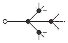
Figure 6.

Definition 3.1.

A subgraph of the Schreier graph $X$ isomorphic to a branch in the Cayley graph of $F$ (with its labelling) is called a hanging branch. The subgraph $X_{*}\subset X$ obtained by removing from $X$ all the hanging branches (i.e., all their edges and all the interior vertices) is called the core of $X$.

With the exception of the trivial case when the Schreier graph $X$ is a tree, i.e., $H=\{e\}$ (which we shall always exclude below), the core $X_{*}$ is non-empty. Any hanging branch is contained in a unique maximal hanging branch, and maximal hanging branches are precisely those whose root belongs to the core. In other words, the graph $X$ is obtained from the core $X_{*}$ by filling the deficient valencies of the vertices of $X_{*}$ with maximal hanging branches (so that all the degrees of the resulting graph have the full valency $|{\breve{\mathcal{A}}}|$). Thus, since the Schreier graph $X$ is connected, its core $X_{*}$ is also connected.

Remark 3.2.

The definition of the core of a graph as what is left after removing all the subtrees is due to Gersten [Ger83, Sta83]. See [Sta91, KM02] for an exposition of the ensuing approach of Stallings to the study of subgroups of free groups based on the notion of a folding of graphs. Note that, following [Sta83, Section 7.2] we are talking about the absolute core of a graph which is independent of the choice of a reference vertex. Some authors (e.g., [BO10]) use a different definition, according to which the (relative) core is the union of all reduced loops in the Schreier graph $X$ starting from a chosen reference point $o\in X$. The absolute and the relative cores coincide if and only if the reference vertex $o$ lies in the absolute core.

The following property is, of course, known to specialists (moreover, it is basically the raison d’être of the definition of the core).

Proposition 3.3.

A subgroup $H\leq F$ is finitely generated if and only if the core $X_{*}$ of the associated Schreier graph $X$ is finite.

Proof.

There is a natural one-to-one correspondence between spanning trees in the Schreier graph $X$ and in the core $X_{*}$. Indeed, the restriction of any spanning tree in $X$ to $X_{*}$ is a spanning tree in $X_{*}$. Conversely, any spanning tree in $X_{*}$ uniquely extends to a spanning tree in $X$ by attaching to it all the maximal hanging branches. Now, if the core is finite, then any spanning tree in it ($\equiv$ the associated spanning tree in $X$) is obtained by removing finitely many edges, so that the number of generators of $H$ is finite (see Theorem 1.8). Conversely, if $H$ is finitely generated, then the core is contained in the finite union of the cycles in $X$ corresponding to the generators of $H$. ∎

The definition of the core directly implies

Lemma 3.4.

All the paths $\varphi\in\mathsf{Paths}_{o}(X)\cup\mathsf{Paths}_{o}^{\infty}(X)$ (i.e., both finite and infinite paths without backtracking issued from $o$) can be uniquely split into the following three consecutive parts (some of which may be missing), see Figure 7:

• the geodesic segment joining the origin $o$ with the root $o^{\prime}\in X_{*}$ of the maximal hanging branch which contains $o$ (if $o\notin X_{*}$ and $\varphi$ passes through $X_{*}$);

• the part of $\varphi$ (possibly infinite) which is contained in $X_{*}$;

• the part of $\varphi$ (possibly infinite) entirely contained inside a certain hanging branch.

\psfrag{o}[rb][rb]{$o$}\psfrag{O}[rb][rb]{$o^{\prime}$}\psfrag{X}[l][l]{$X_{*}$}\includegraphics[scale={.6}]{core.eps}

Figure 7.

Below we shall also use the following

Lemma 3.5.

Let $\mathcal{S}$ be the system of generators of a subgroup $H\leq F$ determined by a spanning tree $T$ in the Schreier graph $X$. Then for any $s\in\mathcal{S}$ the Schreier graph $X^{\prime}$ of the group $H^{\prime}=\langle\mathcal{S}\setminus\{s\}\rangle$ is obtained by deleting from $X$ the edge $\mathcal{E}_{s}$ and attaching a hanging branch to each of its endpoints.

Proof.

Being a Schreier graph, the edges of $X$ are labelled with letters from ${\breve{\mathcal{A}}}$. This labelling extends to a labelling of $X^{\prime}$ which makes of it the Schreier graph of a certain subgroup of $F$. We can choose a spanning tree $T^{\prime}$ in $X^{\prime}$ by taking the union of $T$ and of the hanging branches added during the construction of $X^{\prime}$. The tree $T^{\prime}$ determines then a set of generators $\mathcal{S}^{\prime}$, which, since the labellings of $X$ and $X^{\prime}$ agree, coincides with $\mathcal{S}\setminus\{s\}$. ∎

3.B. The full limit set

Definition 3.6.

The limit set $\Lambda=\Lambda_{H}\subset\partial F$ of a subgroup $H\leq F$ is the set of all the limit points of $H$ with respect to the compactification $\widehat{F}=F\cup\partial F$ described in Section 1.C (below we shall sometimes call this limit set full in order to distinguish it from other limit sets).

The limit set $\Lambda$ is closed and $H$-invariant. The following description is actually valid for an arbitrary discrete group of isometries of a Gromov hyperbolic space, see [Gro87, Bou95]:

Theorem 3.7.

The action of $H$ on $\Lambda$ is minimal (there are no proper $H$-invariant closed subsets), whereas the action of $H$ on the complement $\partial F\setminus\Lambda$ is properly discontinuous (no orbit has accumulation points).

In our concrete situation the limit set $\Lambda$ and a certain natural fundamental domain in $\partial F\setminus\Lambda$ admit the following very explicit description (similar to Proposition 1.18) in terms of the correspondence $\omega\mapsto\pi(\omega)$ between $\partial F$ and the set $\mathsf{Paths}_{o}^{\infty}(X)$ of infinite paths without backtracking in $X$ starting from the origin $o$ (see Proposition 1.3 and the comment before Proposition 1.18).

Theorem 3.8.

• The full limit set $\Lambda\subset\partial F$ corresponds to the set of paths from $\mathsf{Paths}_{o}^{\infty}(X)$ which eventually stay inside the core $X_{*}$ (i.e., for these paths the component (ii) from Lemma 3.4 is infinite).

• The full limit set $\Lambda$ is the closure $\overline{\Omega}$ of the Schreier limit set.

• The complement $\partial F\setminus\Lambda$ is a disjoint union of $H$-translates of the fundamental domain $\Theta=\Delta\cap\left(\partial F\setminus\Lambda\right)$. The set $\Theta$ is open and corresponds to the set of paths from $\mathsf{Paths}_{o}^{\infty}$ which do not pass through any of the edges from $\mathsf{Edges}(X)\setminus\mathsf{Edges}(T)$ and eventually stay inside a hanging branch (i.e., for which the component (iii) from Lemma 3.4 is infinite).

• $\Lambda=\Omega$ (equivalently, $\Delta=\Theta$) if and only if $H$ is finitely generated.

Proof.

(i) Elements of $H$ correspond to cycles in $\mathsf{Paths}_{o}(X)$. By Lemma 3.4, if $o\in X_{*}$ then any cycle from $\mathsf{Paths}_{o}(X)$ is entirely contained in the core, and if $o\notin X_{*}$ then for any such cycle the components (i) and (iii) described in Lemma 3.4 are the geodesic segments $[o,o^{\prime}]$ and $[o^{\prime},o]$, respectively. Thus, the pointwise limit of any sequence of such cycles (as their lengths go to infinity) is a path from $\mathsf{Paths}_{o}^{\infty}(X)$ with infinite component (ii). Conversely, if the $n$-th point $\varphi(n)$ of a path $\varphi\in\mathsf{Paths}_{o}^{\infty}(X)$ belongs to $X_{*}$, then the corresponding truncation $[\varphi]_{n}$ can be extended to a cycle without backtracking (as otherwise $\varphi(n)$ must be inside a hanging branch), so that $\varphi$ is a pointwise limit of cycles from $\mathsf{Paths}_{o}(X)$.

(ii) As it follows from Theorem 1.11, $\Omega\subset\Lambda$, it is non-empty and $H$-invariant. Thus, in view of the minimality of $\Lambda$ (Theorem 3.7), $\overline{\Omega}=\Lambda$.

(iii) Since $\Theta\subset\Delta$, the fact that its $H$-translates are pairwise disjoint and that their union is the complement of $\Lambda$ follows at once from Theorem 1.21. The description of $\Theta$ in terms of the associated subset of $\mathsf{Paths}_{o}^{\infty}(X)$ is a combination of the description of the complement of $\Lambda$, which is (i) above, and of the description of the Schreier fundamental domain $\Delta$ (Proposition 1.18). Finally, $\Theta$ is open because hanging branches contain no edges from $\mathsf{Edges}(X)\setminus\mathsf{Edges}(T)$, so that if a path $\varphi\in\mathsf{Paths}_{o}^{\infty}$ corresponds to a point $\omega\in\Theta$, then the whole open cylinder $C_{[\omega]_{n}}$ is also contained in $\Theta$ for a sufficiently large $n$.

(iv) We shall prove this claim in terms of the descriptions of the sets $\Delta$ and $\Theta$ from Proposition 1.18 and from (iii) above, respectively. Therefore, in view of Proposition 3.3 we have to show that the core $X_{*}$ is finite if and only if all the paths from $\mathsf{Paths}_{o}^{\infty}(X)$ confined to the spanning tree $T$ eventually hit a certain hanging branch. Indeed, if $X_{*}$ is finite, then the restriction of the spanning tree $T$ to $X_{*}$ is also finite, so that any path as above must eventually leave $X_{*}$ and enter a hanging branch. Conversely, if $X_{*}$ is infinite, then the restriction of the spanning tree $T$ to $X_{*}$ is also infinite, so that there is an infinite path without backtracking obtained by first joining $o$ with $X_{*}$ (if $o\notin X_{*}$) and then staying inside the restriction of $T$ to $X_{*}$. ∎

Remark 3.9.

Although the Schreier fundamental domain $\Delta$ is closed (Proposition 1.16) and contains the fundamental domain $\Theta$, it is not necessarily the closure of $\Theta$. For instance, it may happen that $\Theta$ is empty (i.e., $\Lambda=\partial F$), although $\Delta$ is not (and even has positive measure, see Remark 3.12).

Corollary 3.10.

$\Lambda=\partial F$ if and only if the Schreier graph $X$ has no hanging branches (i.e., $X_{*}=X$).

Corollary 3.11.

If $X$ has a hanging branch, then the boundary action of $H$ has a non-trivial dissipative part.

Proof.

If $X$ has a hanging branch, then by Corollary 3.10 $\Lambda\neq\partial F$, i.e., the fundamental domain $\Theta$ is non-empty. Since $\Theta$ is open, and the measure $\mathfrak{m}$ has full support, $\mathfrak{m}\Theta>0$, so that $\Theta$ is a non-trivial wandering set. ∎

Remark 3.12.

The converse of Corollary 3.11 is not true, see Example 4.19.

3.C. Radial limit set

Specializing the type of convergence in the definition of the full limit set (Definition 3.6) one obtains subsets of $\Lambda$ with various geometric properties.

Definition 3.13.

The radial limit set $\Lambda^{rad}\subset\partial F$ is the set of all the accumulation points of the sequences of elements of $H$ which stay inside a tubular neighbourhood of a certain geodesic ray in $F$.

This definition in combination with Theorem 3.8(i) implies

Proposition 3.14.

The radial limit set $\Lambda^{rad}\subset\partial F$ corresponds to the set of paths $\varphi\in\mathsf{Paths}_{o}^{\infty}(X)$ which eventually stay inside the core $X_{*}$ and do not go to infinity (i.e., $\liminf_{n}d_{X}(o,\varphi(n))<\infty$).

Proposition 3.15.

The radial limit set $\Lambda^{rad}$ coincides with the full limit set $\Lambda$ if and only if the group $H$ is finitely generated.

Proof.

By Proposition 3.3, $H$ is finitely generated if and only if the core $X_{*}$ is finite, which implies the claim in view of Proposition 3.14. ∎

Remark 3.16.

According to a result of Beardon and Maskit [BM74], a Fuchsian group is finitely generated if and only if its limit set is the union of the radial limit set and the set of parabolic fixed points. In our situation there are no parabolic points, so that Proposition 3.15 is a complete analogue of this result. In other words, a subgroup of a finitely generated free group is geometrically finite (see [Bow93]) if and only if it is finitely generated. Note that the core can also be defined as the quotient of the geodesic convex hull of the full limit set $\Lambda$ by the action of $H$, so that in our situation geometrical finiteness of $H$ coincides with its convex cocompactness (i.e., finiteness of the core).

3.D. Horospheric limit sets

Definition 3.17.

The horosphere passing through a point $g\in F$ and centered at a point $\omega\in\partial F$ is the corresponding level set of the Busemann cocycle $\beta_{\omega}$:

$$\operatorname{Hor}_{\omega}(g)=\{g^{\prime}\in F:\beta_{\omega}(g,g^{\prime})=0\}\;.$$

In the same way, the horoballs in $F$ are defined as

$$\operatorname{HBall}_{\omega}(g)=\{g^{\prime}\in F:\beta_{\omega}(g,g^{\prime})\leq 0\}\;.$$

Restricting converging sequences to horoballs in $F$ provides us with horospheric limit points. Unfortunately, the situation here is more complicated than with the radial limit points, and we have to define two different horospheric limit sets.

Definition 3.18.

The small (resp., big) horospheric limit set $\Lambda^{horS}=\Lambda^{horS}_{H}$ (resp., $\Lambda^{horB}=\Lambda^{horB}_{H}$) of a subgroup $H\leq F$ is the set of all the points $\omega\in\partial F$ such that any (resp., a certain) horoball centered at $\omega$ contains infinitely many points from $H$.

In terms of the Busemann function a point $\omega\in\partial F$ belongs to $\Lambda^{horS}$ (resp., to $\Lambda^{horB}$) if for any (resp., a certain) $N\in\mathbb{Z}$ there are infinitely many points $h\in H$ with $b_{\omega}(h)\leq N$.

Remark 3.19.

Usually our small horospheric limit set is called just the horospheric limit set, and in the context of Fuchsian and Kleinian groups its definition, along with the definition of the radial limit set, goes back to Hedlund [Hed36]. Following [Mat02] we call it small in order to better distinguish it from the big one, which, although apparently first explicitly introduced by Tukia [Tuk97], essentially appears already in Pommerenke’s paper [Pom76]. See [Sta95, DS00] for a detailed discussion of various kinds of limit points for Fuchsian groups.

The horospheric limit sets $\Lambda^{horS},\Lambda^{horB}$ are obviously $H$-invariant and contained in the full limit set $\Lambda$ (since the only boundary accumulation point of any horoball is just its center). The following theorem describes the relationship between the full limit set $\Lambda$, the radial limit set $\Lambda^{rad}$, the both horospheric limit sets, the Schreier limit set $\Omega$ and the set $\Sigma$ (2.13).

Theorem 3.20.

One has the inclusions

$$\Lambda^{rad}\subset\Lambda^{horS}\subset\Omega\subset\Lambda^{horB}\subset\Sigma\subset\Lambda\;.$$

Proof.

$\Lambda^{rad}\subset\Lambda^{horS}$. Obvious.

$\Lambda^{horS}\subset\Omega$. It follows from Theorem 1.21 and Proposition 2.10.

$\Omega\subset\Lambda^{horB}$. This inclusion was actually already established in the course of the proof of Theorem 2.12.

$\Lambda^{horB}\subset\Sigma$. Obvious.

$\Sigma\subset\Lambda$. Clearly, we may assume that $\Lambda\neq\partial F$. If $\omega\notin\Lambda$, then $\max_{h\in H}(h|\omega)<\infty$ (for, if $(h_{n}|\omega)\to\infty$, then $h_{n}\to\omega$). Thus, by formula (2.5) for any $\omega\notin\Lambda$ convergence of the series (2.13) from the definition of the set $\Sigma$ is equivalent to convergence of the Poincaré series $\sum_{h\in H}(2m-1)^{-|h|}$. Now, if $\Lambda\neq\partial F$, then by Corollary 3.10 and Corollary 3.11 the boundary action has a non-trivial dissipative part, and the Poincaré series is convergent by Corollary 3.36 below. ∎

We shall show in Section 3.G later on that all the inclusions in Theorem 3.20 are, generally speaking, strict. Nonetheless,

Theorem 3.21.

The sets $\Lambda^{horS},\Omega,\Lambda^{horB},\Sigma$ all coincide $\mathfrak{m}$-mod 0.

Proof.

As it follows from Theorem 2.2, Proposition 2.6 and Theorem 2.12, the sets $\Sigma$ and $\Omega$ coincide $\mathfrak{m}$-mod 0. We shall show that $\mathfrak{m}(\Lambda^{horB}\setminus\Lambda^{horS})=0$ which would imply the claim. Indeed, on the $H$-invariant set $A=\Lambda^{horB}\setminus\Lambda^{horS}$, which is contained (mod 0) in the conservative part of the action, the projection $\widetilde{\partial F}\cong\partial F\times\mathbb{Z}\to\partial F$ admits a measurable $H$-equivariant section (which consists in assigning to a boundary point $\omega$ the “smallest” horosphere centered at $\omega$ and containing an infinite number of points from $H$). It implies that the ergodic components of the skew action of $H$ on $A\times\mathbb{Z}\subset\widetilde{\partial F}$ are given by taking this section and its shifts over the ergodic components of the action of $H$ on $A$, the latter being impossible by Theorem 3.38 on a set of positive measure. ∎

Remark 3.22.

Coincidence (mod 0) of the conservative part of the boundary action with the big horospheric limit set $\Lambda^{horB}$ is actually true in much greater generality of an arbitrary Gromov hyperbolic space endowed with a quasi-conformal boundary measure [Kai10]. The proof uses the fact that, by definition, the logarithms of the Radon–Nikodym derivatives of this measure are (almost) proportional to the Busemann cocycle, in combination with the criterion from Theorem 2.2.

3.E. Boundary action and random walks

An important aspect of the boundary behaviour is related to the asymptotic properties of random walks on the group $F$ and on the Schreier graph $X$ (see [KV83, Kai00b] and the references therein for the general background), and, in particular, to the fact that the uniform measure on the boundary $\mathfrak{m}$ can be interpreted as the harmonic measure of the simple random walk on $F$.

Let $\mu$ be the probability measure on the group $F$ equidistributed on the generating set ${\breve{\mathcal{A}}}$. Then the random walk $(F,\mu)$ is precisely the simple random walk on the Cayley graph $\Gamma(F,{\breve{\mathcal{A}}})$, i.e., for any $g\in F$ the transition probability $\pi_{g}=g\mu$ is equidistributed on the set of neighbors of $g$ in the graph $\Gamma(F,{\breve{\mathcal{A}}})$. Moreover, at each point $g\in F$ the increment $\zeta\in{\breve{\mathcal{A}}}$ is precisely the label of the edge along which the random walk moves to a new position.

The following result (which we reformulate in modern terms) is due to Dynkin and Maljutov [DM61]:

Theorem 3.23.

Sample paths of the simple random walk $(F,\mu)$ converge a.e. to the boundary $\partial F$, the hitting distribution is the uniform measure $\mathfrak{m}$, and the space $(\partial F,\mathfrak{m})$ is isomorphic to the Poisson boundary of this random walk.

There is an obvious one-to-one correspondence between the harmonic functions of the simple random walk on the Schreier graph $X$ (the definition of which — the same as for the simple random walk $(F,\mu)$ — takes into account eventual loops and multiple edges in $X$) and $H$-invariant $\mu$-harmonic functions on $F$. This situation is a very specific case of a general theory of covering Markov operators developed in [Kai95]. In particular, [Kai95, Theorem 2.1.4] implies:

Theorem 3.24.

The space of ergodic components of the action of $H$ on $(\partial F,\mathfrak{m})$ is canonically isomorphic to the Poisson boundary of the simple random walk on the Schreier graph $X$. In particular, the action is ergodic if and only if this random walk is Liouville ($\equiv$ has no non-constant bounded harmonic functions).

Yet another corollary of the general theory (see [Kai95, Theorem 3.3.3]) is

Theorem 3.25.

The action of any non-trivial normal subgroup $H\lhd F$ on $(\partial F,\mathfrak{m})$ is conservative.

Remark 3.26.

A similar result in the hyperbolic setup is due to Matsuzaki: the boundary action of any normal subgroup of a divergent type discrete group $G$ of isometries of the hyperbolic space $\mathbf{H}^{d+1}$ is conservative with respect to the associated Patterson measure class. It was first established when the critical exponent $\delta$ of the group $G$ is $d$ (i.e., the corresponding Patterson measure class coincides with the boundary Lebesgue measure class) [Mat93], and later extended to the case of an arbitrary $\delta$ [Mat02]. For $\delta\geq d/2$ this result also readily follows from the theory of covering Markov operators [Kai95, Theorem 4.2.4].

The situation when $\mathfrak{m}\Lambda=0$ can be completely characterized in terms of the simple random walk on the Schreier graph.

Proposition 3.27.

$\mathfrak{m}\Lambda=0$ if and only if a.e. sample path of the simple random walk on $X$ eventually stays inside a certain hanging branch.

Proof.

Using the labelling of edges, any sample path $(x_{n})$ of the simple random walk on $X$ can be uniquely lifted to a sample path $(g_{n})$ of the simple random walk on $F$. The latter a.e. converges to a boundary point $\omega\in\partial F$, and the distribution of $\omega$ is precisely the measure $\mathfrak{m}$ (Theorem 3.23). A sample path $(x_{n})$ eventually stays inside a hanging branch if and only if the path $\pi(\omega)$ does so, whence the claim in view of Theorem 3.8(i). ∎

Corollary 3.28.

If the simple random walk on the Schreier graph $X$ is such that a.e. sample path eventually stays inside a certain hanging branch, then the boundary action is completely dissipative.

Remark 3.29.

The converse of Corollary 3.28 is not true, see Example 4.19.

Corollary 3.11 implies that the boundary action of any finitely generated group $H$ of infinite index has a non-trivial dissipative part. Indeed, since $H$ is finitely generated, the core $X_{*}$ of the Schreier graph $X$ is finite (Proposition 3.3). As $H$ is of infinite index, the graph $X$ is infinite and so necessarily has a hanging branch.

In fact, the following dichotomy completely describes the conservativity properties of the boundary action for finitely generated groups:

Theorem 3.30.

If $H$ is finitely generated, then the Hopf alternative holds: either

• $H$ is of finite index and its boundary action is ergodic (therefore, conservative),

or

• $H$ is of infinite index and its boundary action is completely dissipative.

Proof.

If a subgroup $H$ has a finite index, then the associated Schreier graph $X$ is finite, and therefore the simple random walk on it is Liouville, so that the boundary action of $H$ is ergodic by Theorem 3.24.

If $H$ is finitely generated of infinite index, then $X$ in an infinite graph consisting of a finite core $X_{*}$ and some hanging branches glued to it (see Proposition 3.3). Since the simple random walk in any hanging branch is transient, the simple random walk on $X$ is also transient, which implies that a.e. sample path eventually stays inside a certain hanging branch, whence the claim by Corollary 3.28. ∎

Remark 3.31.

In view of Proposition 3.27 the dichotomy from Theorem 3.30 can be reformulated in the following way: for a finitely generated group $H$ either the Schreier graph $X$ is finite, or else $\mathfrak{m}\Lambda=0$.

Remark 3.32.

For infinitely generated subgroups this dichotomy does not hold, for instance, see Example 4.27.

Remark 3.33.

An unexpected application of Theorem 3.30 is a one line conceptual proof of an old theorem of Karrass and Solitar [KS57]: if $H\leq F$ is finitely generated and contains a non-trivial normal subgroup, then $H$ is of finite index in $F$ (if $H$ itself is a normal subgroup, this was first proved by Schreier in his famous 1927 paper [Sch27]). Indeed, if $H$ contains a normal subgroup, then its boundary action is conservative by Theorem 3.25 and Remark 2.1. Since $H$ is finitely generated, by Theorem 3.30 it must be of finite index in $F$. Note that a recent far-reaching generalization of the Karrass–Solitar theorem [PT07, Corollary 5.13] in particular extends it to all subgroups $H\leq F$ with the property that the set $gH\cap Hg$ is infinite for all $g\in F$. It would be interesting to compare this property with the conservativity of the boundary action.

Remark 3.34.

Any infinitely generated subgroup $H$ of infinite index with conservative boundary action readily provides the following example: the action of any finitely generated subgroup of $H$ is completely dissipative by Theorem 3.30 in spite of conservativity of the action of the whole group $H$.

3.F. Extensions of the boundary action

There are two extensions of the boundary action which have natural geometric interpretations. The first one is the action of $H$ on the space $\partial^{2}F:=(\partial F\times\partial F)\setminus\operatorname{diag}$, or, in other words, on the space of bi-infinite geodesics in the Cayley graph $\Gamma(F,{\breve{\mathcal{A}}})$. We shall endow it with the square $\mathfrak{m}^{2}$ of the measure $\mathfrak{m}$.

Ergodicity of this action is equivalent to ergodicity of the (discrete) geodesic flow on $X$. The study of the ergodic properties of the action of a discrete group of hyperbolic isometries of $\mathbb{H}^{n}$ on $\partial^{2}\mathbb{H}^{n}$ has a long history beginning with the pioneering works of Hedlund and E. Hopf in the 30’s for Fuchsian groups. Its current state is given by the so-called Hopf–Tsuji–Sullivan theorem, e.g., see [Sul81, Nic89, Kai94] and the references therein. Analogous results for the action of a subgroup $H$ of a free group on $\partial^{2}F$ with respect to the measure $\mathfrak{m}^{2}$ were obtained by Coornaert and Papadopoulos [CP96, Corollaire D]. The results from [CP96] actually follow from more general considerations of Kaimanovich [Kai94, Theorem 3.3 and the discussion in Section 3.3.3], where the general case of the harmonic measure of a covering Markov operator on a Gromov hyperbolic space was treated. In our situation these results can be summarized as the following analogue of the Hopf–Tsuji–Sullivan theorem:

Theorem 3.35 ([Kai94, CP96]).

The action of $H$ on $(\partial^{2}F,\mathfrak{m}^{2})$ is either ergodic (therefore, conservative) or completely dissipative (the Hopf alternative). If the action is ergodic, then

• $\mathfrak{m}\Lambda^{rad}=1$;

• The simple random walk on the Schreier graph $X$ is recurrent;

• The Poincaré series $\sum_{h\in H}(2m-1)^{-|h|}$ diverges.

Alternatively, if the action is completely dissipative, then

• $\mathfrak{m}\Lambda^{rad}=0$;

• The simple random walk on the Schreier graph $X$ is transient;

• The Poincaré series converges.

Corollary 3.36.

If the action of $H$ on $(\partial F,\mathfrak{m})$ is dissipative, then the Poincaré series converges.

Proof.

Since the action of $H$ on $(\partial^{2}F,\mathfrak{m}^{2})$ projets to the action on $(\partial F,\mathfrak{m})$, dissipativity of the latter implies dissipativity of the former. ∎

Remark 3.37.

The action of $F$ on $\partial^{3}F$ (and therefore on all the higher products) is properly discontinuous in view of the existence of an equivariant barycenter map $\partial^{3}F\to F$. Hence, it is dissipative for any purely non-atomic measure.

Yet another extension of the boundary action is obtained by taking the skew action of $H$ on $\widetilde{\partial F}:=\partial F\times\mathbb{Z}$ determined by the Busemann cocycle. Geometrically this action is just the action of $H$ on the space of horospheres in $F$ (see Section 3.D). The space $\widetilde{\partial F}$ is endowed with the natural measure $\widetilde{\mathfrak{m}}$ which is the product of $\mathfrak{m}$ and the counting measure on $\mathbb{Z}$. The ergodic properties of this action essentially coincide with the ergodic properties of the boundary action, namely:

Theorem 3.38.

Let $\partial F=\mathcal{C}\cup\mathcal{D}$ be the decomposition of the boundary $\partial F$ into the conservative and the dissipative parts of the $H$-action. Then the conservative and the dissipative parts of the action of $H$ on the space $\widetilde{\partial F}$ are $\mathcal{C}\times\mathbb{Z}$ and $\mathcal{D}\times\mathbb{Z}$, respectively. The conservative ergodic components of the $H$-action on $\widetilde{\partial F}$ are the preimages of the ergodic components of the $H$-action on $\mathcal{C}$ under the projection $\widetilde{\partial F}\to\partial F$. In particular, the action of $H$ on $\mathcal{C}\times\mathbb{Z}$ is ergodic if and only if the action of $H$ on $\mathcal{C}$ is ergodic.

The proof of this theorem almost verbatim coincides with the proof of the analogous result for the boundary actions of Fuchsian groups [Kai00a, Theorem 4.2] based in turn on Sullivan’s proof in [Sul82] (see also [Sul81]) of the fact that the boundary action of a Kleinian group is of type $\textup{III}_{1}$ on its conservative part with respect to the Lebesgue measure. The only difference is that in our situation the range of the Busemann cocycle is $\mathbb{Z}$ (rather than $\mathbb{R}$ as in the case of manifolds), so that, in particular, the type of the boundary action of $H$ on the conservative part is $\textup{III}_{\lambda}$ with $\lambda=\log(2m-1)$.

3.G. Examples

We shall now give examples showing that all the sets from Theorem 3.20 are, in general, pairwise distinct.

Example 3.39.

$\Lambda^{rad}\neq\Lambda^{horS}$. By Theorem 2.12, Theorem 3.21, Theorem 3.24 and Theorem 3.35, if the simple random walk on $X$ is transient, but still has the Liouville property, then $\mathfrak{m}\Lambda^{rad}=0$, whereas $\mathfrak{m}\Lambda^{horS}=1$. Such examples are readily available already in the case when the subgroup $H$ is normal and $X$ is the quotient group, see [KV83].

Example 3.40.

$\Lambda^{horS}\neq\Omega$. Let us take two geodesic rays $\rho_{1},\rho_{2}\cong\mathbb{Z}_{+}$ joined at the origin $o$, so that $\rho_{1}(0)=\rho_{2}(0)=o$. We construct the Schreier graph $X$ by first adding the edges $[\rho_{1}(n+1),\rho_{2}(n)]$ for all $n>0$ and then filling all the deficient valencies with hanging branches. The geodesic spanning tree $T$ is obtained from $X$ by removing all the edges $[\rho_{1}(n),\rho_{1}(n+1)]$ for $n>0$, see Figure 8. Let $\omega_{1}\in\partial F$ be the boundary point which corresponds to the ray $\rho_{1}$ considered as a path without backtracking in $X$. Then $\omega_{1}\in\Omega$ because $\rho_{1}$ passes through an infinite number of edges from $\mathsf{Edges}(X)\setminus\mathsf{Edges}(T)$. On the other hand, since $\omega_{1}$ corresponds to a geodesic in $X$, $\omega\notin\Lambda^{horS}$ by Proposition 2.11.

\psfrag{o}[tr][tr]{$o$}\psfrag{r1}[Bl][Bl]{$\rho_{1}(n+1)$}\psfrag{r2}[tl][tl]{$\rho_{2}(n)$}\psfrag{o1}[tl][l]{$\omega_{1}$}\psfrag{o2}[tl][l]{$\omega_{2}$}\includegraphics[scale={.75}]{ex17.eps}

Figure 8.

Example 3.41.

$\Omega\neq\Lambda^{horB}$. Let $X$ be the same graph as in the previous example. Take the boundary point $\omega_{2}\in\partial F$ which corresponds this time to the ray $\rho_{2}$, see Figure 8. Then $\omega_{2}\notin\Omega$. On the other hand, for any $n>0$ the generator $s_{n}$ corresponding to the edge $[\rho_{1}(n),\rho_{1}(n+1)]$ has the property that $b_{\omega_{2}}(s_{n})=2$, whence $\omega_{2}\in\Lambda^{horB}$.

Example 3.42.

$\Lambda^{horB}\neq\Sigma$. Let us take a geodesic ray $\rho\cong\mathbb{Z}_{+}$ starting at the origin $o=\rho(0)$ and an integer sequence $d_{n}$ (to be specified later). We construct the Schreier graph $X$ by first attaching to each vertex $\rho(n),\,n>0,$ a loop of length $2d_{n}+1$ and then filling all the deficient valencies with hanging branches. The spanning geodesic tree $T$ is obtained by removing from each such loop the middle edge $\mathcal{E}_{n}$, so that in $T$ there are two segments of length $d_{n}$ attached to each point $\rho(n)$, see Figure 9. Denote by $s_{n}$ the corresponding generators. Let $\omega\in\partial F$ be the boundary point corresponding to the ray $\rho$. Then for any $h\in H\cong\breve{\mathcal{S}}^{*}_{r}$ one has the inequality $b_{\omega}(h)\geq\sum_{n}t_{n}(2d_{n}+1)$, where $t_{n}$ is the number of occurrences of $s_{n}^{\pm 1}$ in $h$. Indeed, by (2.5) $b_{\omega}(h)=|h|-2(h|\omega)$. We can write $|h|=l+\sum_{n}t_{n}(2d_{n}+1)$, where $l$ is the sum of the lengths of the pieces of the associated path in $X$ which correspond to moving along the ray $\rho$. The latter sum contains the term $(h|\omega)$ which corresponds to the confluent of $h$ and $\rho$, and, since $h$ is a cycle, one has $l\geq 2(h|\omega)$, which implies the desired inequality. Now, if $d_{n}\uparrow\infty$, then $\omega\notin\Lambda^{horB}$. On the other hand, $b_{\omega}(s_{n})=2d_{n}+1$, and one can still choose $d_{n}$ is such a way that $\sum_{n}(2m-1)^{-2d_{n}}=\infty$, so that $\omega\in\Sigma$.

\psfrag{o}[tr][tr]{$o$}\psfrag{r1}[t][t]{$\rho(1)$}\psfrag{r2}[t][t]{$\rho(n)$}\psfrag{E1}[b][b]{$\mathcal{E}_{1}$}\psfrag{E2}[b][b]{$\mathcal{E}_{n}$}\psfrag{o2}[tl][l]{$\omega$}\includegraphics[scale={.75}]{ex19.eps}

Figure 9.

Example 3.43.

$\Sigma\neq\Lambda$. Since $\Sigma$ coincides (mod 0) with the conservative part of the action (see Theorem 3.21), whenever the boundary action is completely dissipative we have $\mathfrak{m}\Sigma=0$. On the other hand, in this situation it is still possible that $\Lambda=\partial F$, i.e., that the Schreier graph has no hanging branches (Corollary 3.10), see Example 4.19.

4. Geometry of the Schreier graph

In this Section we shall study the relationship between the ergodic properties of the action of the subgroup $H$ on the boundary $(\partial F,\mathfrak{m})$ and the geometry of the Schreier graph $X=H\backslash F$ (in particular, its quantitative characteristics).

4.A. Growth and cogrowth

Denote by $S_{F}^{n}$ and $B_{F}^{n}$ (resp., $S_{X}^{n}$ and $B_{X}^{n}$) the sphere and the ball of radius $n$ in the Cayley graph $\Gamma(F,{\breve{\mathcal{A}}})$ (resp., in the Schreier graph $X=\Gamma(H\backslash F,{\breve{\mathcal{A}}})$) centered at the group identity $e$ (resp., at the point $o=H$). The exponential volume growth rate of $X$ is

$$v_{X}=\limsup\left|B_{X}^{n}\right|^{1/n}\leq v_{F}=2m-1\;.$$

The cogrowth rate of $X$ ($\equiv$ the growth rate of $H$ in $F$) is

$$v_{H}=\limsup_{n\to\infty}\left|H\cap B_{F}^{n}\right|^{1/n}\leq 2m-1\;,$$

and it is the inverse of the radius of convergence of the cogrowth series

$$\mathcal{G}_{H}(z)=\sum_{n}|H\cap S_{F}^{n}|z^{n}\;.$$

Denote by $\rho_{F}$ (resp., $\rho_{X}$) the spectral radius of the simple random walk on $F$ (resp., on $X=\Gamma(H\backslash F,{\breve{\mathcal{A}}})$), so that $\sqrt{2m-1}/m=\rho_{F}\leq\rho_{X}\leq 1$ [Kes59]. By [Gri78, Gri80]

(4.1) $$\rho_{X}=\left\{\begin{array}[]{ll}\frac{\sqrt{2m-1}}{m}&,\quad 1\leq v_{H}\leq\sqrt{2m-1}\;,\vphantom{\text{\Huge(}}\\ \frac{\sqrt{2m-1}}{2m}\left(\frac{\sqrt{2m-1}}{v_{H}}+\frac{v_{H}}{\sqrt{2m-1}}\right)&,\quad\sqrt{2m-1}\leq v_{H}\leq 2m-1\;,\vphantom{\text{\Huge(}}\\ \end{array}\right.$$

which implies that $\rho_{X}=\rho_{F}$ if and only if $v_{H}\leq\sqrt{2m-1}$, and $\rho_{X}=1$ (i.e., the graph $X$ is amenable) if and only if $v_{H}=2m-1$. Recall that an infinite connected $(2m)$-regular graph $X$ is called Ramanujan if $\rho_{X}=\sqrt{2m-1}/m$. Therefore, a Schreier graph $X=H\backslash F$ is Ramanujan if and only if the growth of the corresponding subgroup $H\leq F$ satisfies the inequality $v_{H}\leq\sqrt{2m-1}$.

4.B. Dissipativity

Theorem 4.2.

If $v_{H}<\sqrt{2m-1}$ then the boundary action of $H$ is completely dissipative.

Proof.

For $h=s_{1}s_{2}\dots s_{n}\in\breve{\mathcal{S}}_{r}^{*}\cong H$ let $C_{h}\subset\partial H$ be the corresponding cylinder set, so that

$$\Omega=\bigcup_{h\in H}\sigma^{\infty}(C_{h})\;.$$

By (1.14)

$$\sigma^{\infty}(C_{h})\subset C_{g}\;,$$

where $C_{g}\subset\partial F$ is the cylinder set based at the word

$$g=\sigma_{-}(s_{1})\sigma_{0}(s_{1})\alpha(s_{1},s_{2})\sigma_{0}(s_{2})\dots\alpha(s_{n-1},s_{n})\sigma_{0}(s_{n})\in{\breve{\mathcal{A}}}^{*}_{r}\cong F\;.$$

Since $|g|\geq|\sigma(h)|/2$ (see the first half of the proof of Proposition 2.9),

$$\mathfrak{m}\sigma^{\infty}(C_{h})\leq\mathfrak{m}C_{g}=\frac{1}{2m(2m-1)^{|g|-1}}\leq\frac{1}{(2m-1)^{|\sigma(h)|/2}}\;,$$

whence

$$\sum_{h\in H}\mathfrak{m}\sigma^{\infty}(C_{h})<\infty\;,$$

which implies the claim by Borel–Cantelli lemma, because any point from $\partial H$ belongs to infinitely many cylinders $C_{h}$. ∎

Remark 4.3.

The converse of Theorem 4.2 is not true, see Example 4.25.

Remark 4.4.

The upper bound $\sqrt{2m-1}$ in Theorem 4.2 is optimal. Indeed, if $N\lhd F$ is a non-trivial normal subgroup, then its boundary action is always conservative, see Theorem 3.25. On the other hand, $N$ being non-amenable, $\rho_{F/N}>\rho_{F}$ by Kesten’s theorem [Kes59], whence by formula (4.1) $v_{N}>\sqrt{2m-1}$. There are numerous examples of normal subgroups $N$ for which $\rho_{F/N}$ is arbitrarily close to $\rho_{F}$, and therefore by (4.1) $v_{N}$ is arbitrarily close to $\sqrt{2m-1}$. For instance, if $N_{l}$ is the kernel of the natural homomorphism $F=\mathbb{Z}*\mathbb{Z}*\dots*\mathbb{Z}\to\mathbb{Z}_{l}*\mathbb{Z}_{l}*\dots*\mathbb{Z}_{l}$, then $\rho_{F/N_{l}}\to\rho_{F}$ as $l\to\infty$ by explicit formulas from [Woe00, Section 9].

Remark 4.5.

We do not know whether there exist subgroups $H\leq F$ whose boundary action is not completely dissipative (or, even better, is conservative), but $v_{H}=\sqrt{2m-1}$. The forthcoming paper [AGV11] contains a family of examples of subgroups with $v_{H}=\sqrt{2m-1}$ (described in terms of the associated Schreier graphs). However, for all these examples the action of $H$ is completely dissipative, because the corresponding Schreier graphs satisfy condition of Proposition 3.27. It is also the case when the Schreier graph $X$ is radially symmetric. [For, then the radial part of the simple random walk on $X$ would also have spectral radius $\rho_{F}$ and would therefore have a positive $\rho_{F}$-invariant function, e.g., see [MW89] and the references therein. On the other hand, an explicit calculation shows that if such a function exists, then the number of cycles in $X$ must be finite, and therefore the action must be completely dissipative by Theorem 3.30.]

Remark 4.6.

Results similar to Theorem 4.2 are known for Fuchsian groups (where completely different methods were used). The fact that if the critical exponent $\delta=\delta_{H}$ ($\equiv$ the logarithmic rate of growth with respect to the Riemannian metric) of a Fuchsian group $H$ satisfies inequality $\delta<\frac{1}{2}$, then the boundary action is completely dissipative with respect to the Lebesgue measure class goes back to Patterson [Pat77]. Another proof is given in a recent paper of Matsuzaki [Mat05], where examples of Fuchsian groups with conservative boundary action for which $\delta$ is arbitrarily close to $\frac{1}{2}$ are constructed. However, it is unknown whether such an example exists with the critical exponent precisely $\frac{1}{2}$ (cf. Remark 4.4).

4.C. Conservativity

Denote by $\gamma(x)$ the number of edges from the set $\mathsf{Edges}(X)\setminus\mathsf{Edges}(T)$ incident with a vertex $x\in X$, so that the degree of $x$ in the spanning tree $T$ is

(4.7) $$\deg_{T}(x)=\deg_{X}(x)-\gamma(x)=2m-\gamma(x)\;.$$

Proposition 4.8.

(4.9) $$\mathfrak{m}\Delta\ =1-\frac{1}{2m}\sum_{x\in X}\frac{\gamma(x)}{(2m-1)^{|x|}}\;.$$

Proof.

By Proposition 1.19 and Theorem 1.21

$$\partial F\setminus\Delta=\bigsqcup_{s\in\breve{\mathcal{S}}}C_{\sigma_{-}(s)\sigma_{0}(s)}\;,$$

whence by formula (2.3)

$$\mathfrak{m}\Delta=1-\frac{1}{2m}\sum_{s\in\breve{\mathcal{S}}}\frac{1}{(2m-1)^{|\sigma_{-}(s)|}}\;,$$

which implies the claim in view of the one-to-one correspondence between the set $\breve{\mathcal{S}}$ and the oriented edges not in $T$ established in Theorem 1.8. ∎

Theorem 4.10.

The sequence

$$a_{n}=\frac{|S_{X}^{n}|}{|S_{F}^{n}|}=\frac{\left|S_{X}^{n}\right|}{2m(2m-1)^{n-1}}$$

monotonically decreases and converges to $\mathfrak{m}\Delta$.

Proof.

By Proposition 4.8

(4.11) $$\mathfrak{m}\Delta=1-\frac{1}{2m}\sum_{n=0}^{\infty}\frac{\gamma_{n}}{(2m-1)^{n}}\;,$$

where

$$\gamma_{n}=\sum_{x\in S_{X}^{n}}\gamma(x)\;.$$

In view of (4.7) the numbers $|S_{X}^{n}|$ and $\gamma_{n}$ are connected by the formulas

$$|S_{X}^{1}|=\deg_{T}o=\deg_{X}o-\gamma_{0}=2m-\gamma_{0}$$

and

$$|S_{X}^{n+1}|=\sum_{x\in S_{X}^{n}}(\deg_{T}x-1)=(2m-1)|S_{X}^{n}|-\gamma_{n}\;,\qquad n>0\;,$$

which imply monotonicity of $a_{n}$. Substituting

$$\gamma_{0}=2m-|S_{X}^{1}|\;,$$

and

$$\gamma_{n}=(2m-1)|S_{X}^{n}|-|S_{X}^{n+1}|\;,\qquad n>0$$

into formula (4.11) yields the claim. ∎

As a corollary we immediately obtain:

Theorem 4.12.

The boundary action of $H$ is conservative if and only if

$$\lim_{n}\frac{|S_{X}^{n}|}{|S_{F}^{n}|}=\lim_{n}\frac{|S_{X}^{n}|}{2m(2m-1)^{n-1}}=0\;.$$

Remark 4.13.

In different terms this result is also independently proved in the recent paper [BO10, Theorem 9].

Corollary 4.14.

If $v_{X}<2m-1$, then the boundary action of $H$ is conservative.

Remark 4.15.

The converse of Corollary 4.14 is not true, see Example 4.26.

Remark 4.16.

Theorem 4.12 can also be reformulated as saying that the boundary action is conservative if and only if $|B_{X}^{n}|/|B_{F}^{n}|\to 0$. In the context of Fuchsian groups this result (obtained by entirely different means) with $B_{F}^{n}$ (resp., $|B_{X}^{n}|$) replaced with the area of the $n$-ball in the hyperbolic plane (resp., in the quotient surface) was proved by Sullivan [Sul81, Theorem IV], and essentially goes back to Hopf [Hop39].

Theorem 4.2 and Theorem 4.12 imply

Corollary 4.17.

If $|S_{X}^{n}|/|S_{F}^{n}|\to 0$ (in particular, if $v_{X}<2m-1$), then $v_{H}\geq\sqrt{2m-1}$.

Remark 4.18.

Since $v_{F/N}<v_{F}$ for any non-trivial normal subgroup $N\lhd F$ (e.g., see [GdlH01]), as another corollary one obtains a “quantitative” proof of Theorem 3.25.

4.D. Examples

Example 4.19 (counterexample to the converse of Corollary 3.11).

The group $H$ is infinitely generated, the graph $X$ has no hanging branches, but $v_{H}$ is arbitrarily close to 1, so that the action of $H$ on $(\partial F,\mathfrak{m})$ is completely dissipative (see Theorem 4.2).

We construct the graph $X$ inductively by starting from the homogeneous tree $X_{0}=T_{2m}$ of degree $2m$ with origin $o$. We shall think of the spheres $S^{R}_{X_{k}}$ centered at $o$ in the graphs $X_{k}$ as levels, and follow the perverse tradition according to which trees are allowed to grow downwards, so that the level 0 (consisting just of the origin) is the highest (actually, in Figure 10 below we shall draw it from left to right). In this construction we shall need an increasing integer sequence $1=d_{1}<d_{2}<\dots$ to be specified later.

The inductive step of the construction consists in choosing two points $x_{k+1}\neq y_{k+1}\in S^{d_{k+1}}_{X_{k}}$ for a certain integer $d_{k+1}$ to be specified later in such a way that their “predecessors” in $S^{d_{k}}_{X_{k}}$ are distinct. The graph $X_{k+1}$ is then obtained from $X_{k}$ in the following way:

• remove from $X_{k}$ one of the branches growing from $x_{k+1}$ downwards;

• do the same with the point $y_{k+1}$;

• add the edge $\mathcal{E}_{k+1}$ joining $x_{k+1}$ and $y_{k+1}$.

Thus, all the graphs $X_{k}$ are also $2m$-regular and have the same origin $o$. Finally, the graph $X$ is the limit of the sequence $X_{k}$, see Figure 10.

\psfrag{o}[rt][rt]{$o$}\psfrag{s1}[t][t]{$S^{d_{1}}$}\psfrag{s2}[t][t]{$S^{d_{2}}$}\psfrag{s3}[t][t]{$S^{d_{3}}$}\psfrag{s4}[t][t]{$S^{d_{4}}$}\psfrag{x2}[B][B]{$x_{2}$}\psfrag{x3}[B][B]{$x_{3}$}\psfrag{x4}[B][B]{$x_{4}$}\psfrag{y2}[t][t]{$y_{2}$}\psfrag{y3}[t][t]{$y_{3}$}\psfrag{y4}[t][t]{$y_{4}$}\psfrag{E2}[r][r]{$\mathcal{E}_{2}$}\psfrag{E3}[r][r]{$\mathcal{E}_{3}$}\psfrag{E4}[r][r]{$\mathcal{E}_{4}$}\includegraphics[scale={.75}]{ex22.eps}

Figure 10.

The graph $X$ has a natural geodesic spanning tree $T$ which is obtained by removing all the horizontal edges $\mathcal{E}_{k}$ added during the construction of $X$. Denote by $s_{k}$ the corresponding generator of $H$, and let $H_{k}=\langle s_{1},s_{2},\dots,s_{k}\rangle$.

Obviously, the sequences of points $x_{k},y_{k}$ can be chosen in such a way that $X$ has no hanging branches as the latter condition is equivalent to the property that the intersection of any shadow in the spanning tree $T$ (with respect to the origin $o$) with the set $\{x_{2},y_{2},x_{3},y_{3},\dots\}$ is non-empty.

We shall now explain (once again inductively) how to choose the sequence $d_{k}$. More precisely, we shall show that once the numbers $d_{1},d_{2},\dots,d_{k}$ and the group $H_{k}$ have already been chosen, and the group $H_{k}$ has the property that

(4.20) $$|H_{k}\cap B_{F}^{n}|\leq C\alpha_{k}^{n}\qquad\forall\,n\geq 0$$

for certain constants $C,\alpha_{k}>1$, then for any $\alpha_{k+1}>\alpha_{k}$ the distance $d_{k+1}$ can be chosen in such a way that for the group $H_{k+1}$ also

(4.21) $$|H_{k+1}\cap B_{F}^{n}|\leq C\alpha_{k+1}^{n}\qquad\forall\,n\geq 0$$

(with the same constant $C$!). Then, starting from the group $H_{1}\cong\mathbb{Z}$ (which has subexponential growth), and taking an arbitrary sequence

$$1<\alpha_{1}<\alpha_{2}<\dots<\alpha_{k}\dots\nearrow\alpha$$

we would be able to conclude that $v_{H}\leq\alpha$.

For notational simplicity we put $s=s_{k+1}$. Any element of the group $H_{k+1}=\langle H_{k},s\rangle$ can be presented as

(4.22) $$g=h_{0}s^{\varepsilon_{1}}h_{1}s^{\varepsilon_{2}}\dots h_{t-1}s^{\varepsilon_{t}}h_{t}$$

for certain $t\geq 0,\,h_{i}\in H$ and $\varepsilon_{i}=\pm 1$ such that $\varepsilon_{i}=\varepsilon_{i+1}$ whenever $h_{i}=e$. As it follows from the definition of $s$, the length of cancellations on each side between any two consecutive terms in the above expansion does not exceed $d_{k}$. Since $|s|=2d_{k+1}+1$, we obtain the inequality

(4.23) $$|g|\geq\sum_{i=0}^{t}|h_{i}|+t|s|-4td_{k}=\sum_{i=0}^{t}|h_{i}|+tD\;,$$

where

(4.24) $$D=|s|-4d_{k}=2d_{k+1}+1-4d_{k}\;.$$

We shall now estimate $|H_{k+1}\cap B_{F}^{n}|$, i.e., the number of elements $g$ of the form (4.22) with $|g|\leq n$, by using the inequality (4.23). We have to control the following numbers:

• The number $t$ of occurrences of $s^{\pm 1}$ in the expansion (4.22);

• The number $N_{b}$ of choices of the signs $\varepsilon_{i}$ for a given value of $t$;

• The number $N_{c}$ of possible sets of lengths $|h_{i}|=l_{i}$ of the words $h_{i}$ for given $t$;

• The number $N_{d}$ of the choices of the words $h_{i}\in H_{k}$ with the prescribed lengths $l_{i}$.

Let us find the corresponding estimates one by one.

(a) By (4.23)

$$t\leq\tau=n/D\;.$$

(b) Trivially,

$$N_{b}\leq 2^{\tau}\;.$$

(c) By (4.23), $N_{c}$ does not exceed the number of ordered partitions of $n-tD$ into not more than $t+1$ integer summands, so that

$$N_{c}\leq\binom{n-tD+t}{t}\;.$$

(d) Finally, by (4.20) and (4.23)

$$N_{d}\leq C^{\tau}\alpha_{k}^{n}\;.$$

Thus,

$$|H_{k+1}\cap B_{F}^{n}|\leq\tau 2^{\tau}\max_{t\leq\tau}\binom{n-tD+t}{t}C^{\tau}\alpha_{k}^{n}\;,$$

and in order to conclude it is sufficient just to estimate the $\max$ in the above product. Since

$$\frac{1}{n}\log\binom{n-tD+t}{t}=\frac{1}{n}\log\binom{n-tD^{\prime}}{t}$$

$$\leq\frac{1}{n}\log\frac{(n-tD^{\prime})^{t}}{(t/e)^{t}}=\frac{t}{n}\left(1+\log\left(\frac{n}{t}-D^{\prime}\right)\right)=\frac{1+\log(z-D^{\prime})}{z}\;,$$

where $D^{\prime}=D-1$ and $z=n/t\geq D$, we can choose $D$ (equivalently, $d_{k+1}$, in view of formula (4.24)) in such a way that

$$\sup_{z\geq D}\frac{1+\log(z-D^{\prime})}{z}$$

is arbitrarily small, whence the claim.

Example 4.25 (counterexample to the converse of Theorem 4.2).

The cogrowth $v_{H}=2m-1$ is maximal, i.e., the Schreier graph $X$ is amenable (see Section 4.A), but the boundary action is completely dissipative.

Take the homogeneous tree $T_{2m}$ with the root $o$, remove one of the branches rooted at $o$, and replace it with a geodesic ray $\rho\cong\mathbb{Z}_{+}$. Then attach to all the vertices of $\rho$ other than the origin $m-1$ length 1 loops, so that the resulting graph $X$ is $2m$-regular: it is a union of $2m-1$ hanging branches and the ray $\rho$ (with attached loops) joined at the point $o$, see Figure 11. The graph $X$ is obviously amenable because of the presence of the $\rho$ branch. On the other hand, the simple random walk on it eventually stays inside one of the hanging branches (since the simple random walk on $\mathbb{Z}_{+}$ is recurrent), whence the claim in view of Corollary 3.28.

\psfrag{o}[rb][rb]{$o$}\includegraphics[scale={.75}]{ex28.eps}

Figure 11.

Example 4.26 (counterexample to the converse of Corollary 4.14).

The growth $v_{X}=2m-1$ is maximal, but the boundary action is conservative.

Take the homogeneous tree $T_{2m}$ with the root $o$ and take an increasing sequence $d_{n}$ with density 0, i.e., such that $d_{n}/n\to\infty$. Then add one new vertex in the middle of each edge of $T_{2m}$ joining the spheres of radii $d_{n}$ and $d_{n}+1$ and attach to every such vertex $m-1$ length 1 loops. Then the resulting graph $X$ is radially symmetric, $2m$-regular, and has the growth $v_{X}=2m-1$, although it satisfies the condition of Theorem 4.12. The radial part of this graph is presented on Figure 12.

\psfrag{o}[rt][rt]{$o$}\psfrag{d}[rb][rb]{$d_{n}$}\psfrag{e}[lb][lb]{$d_{n}+1$}\includegraphics[scale={.75}]{ex29.eps}

Figure 12.

Example 4.27 (counterexample to an extension of Theorem 3.30).

An infinitely generated subgroup $H$ such that its boundary action has both conservative and dissipative parts of positive measure.

Take a group $\widetilde{H}\leq F$ such that the simple random walk on the associated Schreier graph $\widetilde{X}$ is transient and the boundary action of $\widetilde{H}$ is conservative (for instance, this is the case when $\widetilde{H}$ is a normal subgroup with transient quotient, see Theorem 3.25). Then necessarily $\widetilde{H}$ is infinitely generated by Theorem 3.30. Let $\widetilde{\mathcal{S}}$ be the system of generators of $\widetilde{H}$ determined by a geodesic spanning tree $\widetilde{T}$. Then for any $s\in\widetilde{\mathcal{S}}$ the group $H=\langle\mathcal{S}\rangle,\,\mathcal{S}=\widetilde{\mathcal{S}}\setminus\{s\}$ has the desired property.

Indeed, by Lemma 3.5 the Schreier graph $X=H\backslash F$ has hanging branches, which implies that the dissipative part of the boundary action of $H$ is non-trivial (see Corollary 3.11).

Let us now prove non-triviality of the conservative part. Let $\mathcal{E}=\mathcal{E}_{s}\in\mathsf{Edges}(\widetilde{X})\setminus\mathsf{Edges}(\widetilde{T})$ be the edge corresponding to the generator $s$, and let $A\subset\partial F$ be the set of all points $\omega$ such that the associated path $\widetilde{\pi}(\omega)$ in $\widetilde{X}$ never passes through the edge $\mathcal{E}$ (in either direction). Since the boundary action of $\widetilde{H}$ is conservative, by Theorem 2.12 for a.e. point $\omega\in A$ the path $\widetilde{\pi}(\omega)$ passes nonetheless through infinitely many edges not in $\widetilde{T}$.

Transience of the simple random walk implies that $\mathfrak{m}A>0$. Namely, by using labelling along edges every trajectory $(x_{n})$ of the random walk on $X$ lifts to a trajectory $(g_{n})$ of the simple random walk on $F$. Denote by $g_{\infty}\in\partial F$ its limit point. Then the set of edges through which the path $\widetilde{\pi}(g_{\infty})$ passes is contained in the analogous set for the original sample path $(x_{n})$. Thus, if $(x_{n})$ never passes through $\mathcal{E}$, then the path $\widetilde{\pi}(g_{\infty})$ also has this property. By transience the probability of the former event is positive, and since the image of the measure in the space of sample paths under the above transformation is $\mathfrak{m}$, the claim follows.

Now, for any $\omega\in A$ the associated path $\pi(\omega)$ in the Schreier graph $X$ passes through the same edges as the path $\widetilde{\pi}(\omega)$ in $\widetilde{X}$ (under the natural identification described in Lemma 3.5), i.e., it passes through the edges which are not in the spanning tree $T$ of $X$ infinitely many times. Since $\mathfrak{m}A>0$, it means that the conservative part of the boundary action of $H$ is also non-trivial.

Remark 4.28.

One can also show that in the above construction the ergodic components of the boundary action of $\widetilde{H}$ are in one-to-one correspondence with the ergodic components of the conservative part of the boundary action of $H$. In particular, if the boundary action of $\widetilde{H}$ is ergodic, then the conservative part of the boundary action of $H$ is also ergodic. It follows from the fact that the Poisson boundary of the simple random walk on $\widetilde{X}$ does not change after removing the edge $\mathcal{E}$.

Remark 4.29.

In the context of covering Markov operators a similar example with both conservative and dissipative components in the Poisson boundary was constructed in [Kai95].

Remark 4.30.

In the above example the measure $\mathfrak{m}$ of the full limit set $\Lambda$ is intermediate between 0 and 1. Indeed, $\mathfrak{m}\Lambda<1$ because the Schreier graph has a hanging branch. On the other hand, $\mathfrak{m}\Lambda>0$ because the boundary action has a non-trivial conservative part.

5. Associated Markov chains

As we have already seen, the simple random walk on the Schreier graph plays the crucial role in understanding the ergodic properties of the boundary action. In this Section we shall look at two other Markov chains closely connected with the considered problems.

5.A. Random walk on edges

The uniform boundary measure $\mathfrak{m}$ can be interpreted as the measure in the path space of the following Markov chain $(\mathcal{E}_{n})$ on the set of oriented edges of the Schreier graph $X$. Its initial distribution is uniform on the set of $2m$ edges issued from the origin $o$, and the transition probability from an arbitrary edge $\mathcal{E}$ is equidistributed on the set of $2m-1$ edges $\mathcal{E}^{\prime}$ issued from the endpoint of $\mathcal{E}$ without backtracking (in other words, the labels on $\mathcal{E}$ and $\mathcal{E}^{\prime}$ do not cancel). Then Proposition 1.18 and Theorem 2.12 imply

Theorem 5.1.

The boundary action of $H$ is conservative (resp., dissipative) if a.e. sample path of the chain $\mathcal{E}_{n}$ visits the set $\mathsf{Edges}(X)\setminus\mathsf{Edges}(T)$ infinitely often (resp., finitely many times).

Remark 5.2.

Deciding whether a given set is visited or not with positive probability by sample paths of a certain Markov chain is a classical problem in probability (and potential theory) which goes back to Kakutani. Explicit estimates for the probabilities of visiting the set infinitely many times or not visiting it at all are given in terms of various kinds of capacity, see [BPP95].

5.B. Markov chain on cycles

We shall now assume that the conservative part of the action of $H$ on $(\partial F,\mathfrak{m})$ is non-trivial, i.e., $\mathfrak{m}\Omega>0$. We give its symbolic interpretation and show that its ergodicity is equivalent to the Liouville property for a certain naturally associated Markov chain.

Let us endow $\partial H$ with the probability measure $\mathfrak{m}_{*}$ which is the preimage of the normalized restriction $\mathfrak{m}|_{\Omega}/\mathfrak{m}\Omega$ with respect to the map $\sigma^{\infty}$ (see Theorem 1.11). Obviously, the dynamical systems $(H,\Omega,\mathfrak{m}|_{\Omega})$ and $(H,\partial H,\mathfrak{m}_{*})$ are isomorphic (up to the constant multiplier used to normalize the measure $\mathfrak{m}|_{\Omega}$). In particular, the action of $H$ on the space $(\partial H,\mathfrak{m}_{*})$ is conservative.

Recall that the space $\partial H$, being the set of infinite irreducible words in the alphabet $\breve{\mathcal{S}}$, is the state space of a topological Markov chain. The alphabet $\breve{\mathcal{S}}$ of this chain is in one-to-one correspondence with a set of cycles in the Schreier graph $X$ (see Section 1.B).

Theorem 5.3.

The measure $\mathfrak{m}_{*}$ on $\partial H$ is Markov in the alphabet $\breve{\mathcal{S}}$. It corresponds to the initial distribution

$$\theta(s)=\mathfrak{m}_{*}C_{s}\;,\qquad s\in\breve{\mathcal{S}}\;,$$

and the transition matrix

(5.4) $$M(s,s^{\prime})=(2m-1)^{|s^{\prime}|-|ss^{\prime}|}\cdot\frac{\theta(s^{\prime})}{\theta(s)}\;.$$

Proof.

The argument basically consists in noticing that, due to the special properties of the generating set $\mathcal{S}$, the Radon–Nikodym derivative

(5.5) $$\frac{d\mathfrak{m}_{*}(s_{2}s_{3}\dots)}{d\mathfrak{m}_{*}(s_{1}s_{2}s_{3}\dots)}=\frac{ds_{1}\mathfrak{m}_{*}}{d\mathfrak{m}_{*}}(\xi)\;,\quad\xi=s_{1}s_{2}s_{3}\dots\in\partial H\;,$$

of the measure $\mathfrak{m}_{*}$ is Markov in the sense that it depends on the letters $s_{1},s_{2}$ only. [In the language of symbolic dynamics this derivative, or, more rigorously, its logarithm, is called the potential of the measure $\mathfrak{m}$.] Indeed, by Proposition 2.6 and Proposition 2.9

$$\frac{d\mathfrak{m}_{*}(s_{2}s_{3}\dots)}{d\mathfrak{m}_{*}(s_{1}s_{2}s_{3}\dots)}=(2m-1)^{|s_{1}s_{2}|-|s_{2}|}\;,$$

whence for an arbitrary cylinder set $C_{s_{1}s_{2}\dots s_{n}}$

$$\frac{\mathfrak{m}_{*}C_{s_{2}\dots s_{n}}}{\mathfrak{m}_{*}C_{s_{1}s_{2}\dots s_{n}}}=(2m-1)^{|s_{1}s_{2}|-|s_{2}|}\;.$$

Comparing the formula

$$\mathfrak{m}_{*}C_{s_{1}s_{2}\dots s_{n}} =\frac{\mathfrak{m}_{*}C_{s_{1}s_{2}\dots s_{n}}}{\mathfrak{m}_{*}C_{s_{2}\dots s_{n}}}\cdot\frac{\mathfrak{m}_{*}C_{s_{2}\dots s_{n}}}{\mathfrak{m}_{*}C_{s_{3}\dots s_{n}}}\cdot\dots\cdot\frac{\mathfrak{m}_{*}C_{s_{n-1}s_{n}}}{\mathfrak{m}_{*}C_{s_{n}}}\cdot\mathfrak{m}_{*}C_{s_{n}}$$

$$=(2m-1)^{(|s_{2}|-|s_{1}s_{2}|)+(|s_{3}|-|s_{2}s_{3}|)+\dots+(|s_{n}|-|s_{n-1}s_{n}|)}\cdot\theta(s_{n})$$

with the analogous expansion for $\mathfrak{m}_{*}C_{s_{1}s_{2}\dots s_{n}s_{n+1}}$ we get the claim. ∎

5.C. Applications to the boundary action

Theorem 5.6.

The following measure spaces are canonically isomorphic:

• The Poisson boundary of the Markov chain on $\breve{\mathcal{S}}$ described in Theorem 5.3;

• The space of ergodic components of the (one-sided) time shift in the measure space $(\partial H,\mathfrak{m}_{*})$;

• The space of ergodic components of the action of the group $H$ on the measure space $(\partial H,\mathfrak{m}_{*})$.

Proof.

The isomorphism of the spaces (i) and (ii) is a general fact from the theory of Markov chains, e.g., see [Kai92, Definition 1.5], whereas the isomorphism of the spaces (ii) and (iii) follows from the coincidence of the orbit equivalence relations of the time shift and of the $H$-action on $\partial H$. ∎

Remark 5.7.

Of course, Theorem 5.6 remains valid for an arbitrary Markov measure on $\partial H$ with the full support.

Corollary 5.8.

The Schreier graph $X$ is Liouville if and only if the boundary action of $H$ on $(\partial F,\mathfrak{m})$ is conservative and the Markov chain described in Theorem 5.3 is Liouville.

Remark 5.9.

There are examples when the Markov chain described in Theorem 5.3 is Liouville although the Schreier graph $X$ is not. They correspond to the situation when the boundary action of $H$ on $(\partial F,\mathfrak{m})$ has both conservative and dissipative parts, and the conservative part is ergodic, see Example 4.27 and Remark 4.28.

Remark 5.10.

Yet another example of a Markov measure on $\partial H$ is provided by the harmonic (hitting) measure of a random walk $(H,\mu)$ with $\mathop{\text{\rm supp}}\mu=\breve{\mathcal{S}}$. It was known already to Dynkin and Malyutov [DM61] (also see [LM71]), that if $H$ is finitely generated, then the sample paths converge a.e. to the boundary $\partial H$, the hitting measure $\lambda$ is Markov, and the space $(\partial H,\lambda)$ is the Poisson boundary of the random walk $(H,\mu)$. A recent addition to these facts is the observation that the hitting measure $\lambda$ is in fact multiplicative Markov, and not just plain Markov [Mai05, MM07], i.e., the transition probability from any $s\in\breve{\mathcal{S}}$ is the normalized restriction of the initial distribution onto the set $\breve{\mathcal{S}}\setminus\{s^{-1}\}$ of all letters admissible from $s$. These results readily generalize to the situation when $H$ is infinitely generated by using the approximation of $H=\langle s_{1},s_{2},\dots\rangle$ by finitely generated subgroups $H_{n}=\langle s_{1},s_{2},\dots,s_{n}\rangle$. In particular, the hitting measure $\lambda$ on $\partial H$ is just the projective limit of the hitting measures $\lambda_{n}$ on $\partial H_{n}$; since each of the measures $\lambda_{n}$ is multiplicative Markov, the limit measure $\lambda$ is also multiplicative Markov. This fact can be used to show that, generally speaking, the measure $\mathfrak{m}_{*}$ is not equivalent to the hitting measure of a random walk on $H$. Indeed, the Markov measure with the transition probabilities (5.4) is multiplicative only if for any $s^{\prime}\neq s^{\prime\prime}\in\breve{\mathcal{S}}$ the difference $|ss^{\prime}|-|ss^{\prime\prime}|$ is the same for all $s\in\breve{\mathcal{S}}$ with $s^{\prime},s^{\prime\prime}\neq s^{-1}$, which is a quite restrictive condition.

References

- [Aar97] Jon Aaronson, An introduction to infinite ergodic theory, Mathematical Surveys and Monographs, vol. 50, American Mathematical Society, Providence, RI, 1997. MR 1450400 (99d:28025)
- [Abé10] Miklós Abért, Some questions, http://www.renyi.hu/~abert/research/questions.pdf, 2010.
- [AGV11] Miklós Abért, Yair Glasner, and Bálint Virág, The measurable Kesten theorem, in preparation, 2011.
- [BK10] Itai Benjamini and Gady Kozma, Nonamenable Liouville graphs, arXiv:1010.3365v1, 2010.
- [BM74] Alan F. Beardon and Bernard Maskit, Limit points of Kleinian groups and finite sided fundamental polyhedra, Acta Math. 132 (1974), 1–12. MR 0333164 (48 #11489)
- [BO10] Yuri Bahturin and Alexander Olshanskii, Actions of maximal growth, Proc. Lond. Math. Soc. (3) 101 (2010), no. 1, 27–72. MR 2661241
- [Bou95] Marc Bourdon, Structure conforme au bord et flot géodésique d’un -espace, Enseign. Math. (2) 41 (1995), no. 1-2, 63–102. MR 1341941 (96f:58120)
- [Bow93] B. H. Bowditch, Geometrical finiteness for hyperbolic groups, J. Funct. Anal. 113 (1993), no. 2, 245–317. MR 1218098 (94e:57016)
- [BPP95] Itai Benjamini, Robin Pemantle, and Yuval Peres, Martin capacity for Markov chains, Ann. Probab. 23 (1995), no. 3, 1332–1346. MR 1349175 (96g:60098)
- [CFS82] I. P. Cornfeld, S. V. Fomin, and Ya. G. Sinaĭ, Ergodic theory, Grundlehren der Mathematischen Wissenschaften [Fundamental Principles of Mathematical Sciences], vol. 245, Springer-Verlag, New York, 1982, Translated from the Russian by A. B. Sosinskiĭ. MR 832433 (87f:28019)
- [CP96] Michel Coornaert and Athanase Papadopoulos, Récurrence de marches aléatoires et ergodicité du flot géodésique sur les graphes réguliers, Math. Scand. 79 (1996), no. 1, 130–152. MR 1425084 (97i:58135)
- [dlH00] Pierre de la Harpe, Topics in geometric group theory, Chicago Lectures in Mathematics, University of Chicago Press, Chicago, IL, 2000. MR 1786869 (2001i:20081)
- [DM61] E. B. Dynkin and M. B. Maljutov, Random walk on groups with a finite number of generators, Dokl. Akad. Nauk SSSR 137 (1961), 1042–1045. MR 0131904 (24 #A1751)
- [DS00] F. Dal’bo and A. N. Starkov, On a classification of limit points of infinitely generated Schottky groups, J. Dynam. Control Systems 6 (2000), no. 4, 561–578. MR 1778214 (2001f:37060)
- [GdlH01] Rostislav Grigorchuk and Pierre de la Harpe, Limit behaviour of exponential growth rates for finitely generated groups, Essays on geometry and related topics, Vol. 1, 2, Monogr. Enseign. Math., vol. 38, Enseignement Math., Geneva, 2001, pp. 351–370. MR 1929333 (2003h:20078)
- [Ger83] S. M. Gersten, Intersections of finitely generated subgroups of free groups and resolutions of graphs, Invent. Math. 71 (1983), no. 3, 567–591. MR 695907 (85m:05037b)
- [Gri78] R. I. Grigorchuk, Banach invariant means on homogeneous spaces and random walks, Ph.D. thesis, Moscow State University, 1978, in Russian.
- [Gri80] by same author, Symmetrical random walks on discrete groups, Multicomponent random systems, Adv. Probab. Related Topics, vol. 6, Dekker, New York, 1980, pp. 285–325. MR 599539 (83k:60016)
- [Gro87] M. Gromov, Hyperbolic groups, Essays in group theory, Math. Sci. Res. Inst. Publ., vol. 8, Springer, New York, 1987, pp. 75–263. MR 89e:20070
- [Hed36] Gustav A. Hedlund, Fuchsian groups and transitive horocycles, Duke Math. J. 2 (1936), no. 3, 530–542. MR 1545946
- [Hop39] Eberhard Hopf, Statistik der geodätischen Linien in Mannigfaltigkeiten negativer Krümmung, Ber. Verh. Sächs. Akad. Wiss. Leipzig 91 (1939), 261–304. MR 0001464 (1,243a)
- [HR48] Marshall Hall, Jr. and Tibor Radó, On Schreier systems in free groups, Trans. Amer. Math. Soc. 64 (1948), 386–408. MR 0026051 (10,98f)
- [Kai92] Vadim A. Kaimanovich, Measure-theoretic boundaries of Markov chains, - laws and entropy, Harmonic analysis and discrete potential theory (Frascati, 1991), Plenum, New York, 1992, pp. 145–180. MR 94h:60099
- [Kai94] by same author, Ergodicity of harmonic invariant measures for the geodesic flow on hyperbolic spaces, J. Reine Angew. Math. 455 (1994), 57–103. MR 95g:58130
- [Kai95] by same author, The Poisson boundary of covering Markov operators, Israel J. Math. 89 (1995), no. 1-3, 77–134. MR 96k:60194
- [Kai00a] by same author, Ergodic properties of the horocycle flow and classification of Fuchsian groups, J. Dynam. Control Systems 6 (2000), no. 1, 21–56. MR 1738739 (2000m:37033)
- [Kai00b] by same author, The Poisson formula for groups with hyperbolic properties, Ann. of Math. (2) 152 (2000), no. 3, 659–692. MR 1815698 (2002d:60064)
- [Kai10] by same author, Hopf decomposition and horospheric limit sets, Ann. Acad. Sci. Fenn. Math. 35 (2010), no. 2, 335–350. MR 2731695
- [Kes59] Harry Kesten, Symmetric random walks on groups, Trans. Amer. Math. Soc. 92 (1959), 336–354. MR 0109367 (22 #253)
- [KM02] Ilya Kapovich and Alexei Myasnikov, Stallings foldings and subgroups of free groups, J. Algebra 248 (2002), no. 2, 608–668. MR 1882114 (2003a:20039)
- [KS57] A. Karrass and D. Solitar, Note on a theorem of Schreier, Proc. Amer. Math. Soc. 8 (1957), 696–697. MR 0086813 (19,248a)
- [KS58] by same author, Subgroup theorems in the theory of groups given by defining relations., Comm. Pure Appl. Math. 11 (1958), 547–571. MR 0100624 (20 #7053)
- [KV83] V. A. Kaimanovich and A. M. Vershik, Random walks on discrete groups: boundary and entropy, Ann. Probab. 11 (1983), no. 3, 457–490. MR 85d:60024
- [LM71] B. Ja. Levit and S. A. Molčanov, Invariant chains on a free group with a finite number of generators, Vestnik Moskov. Univ. Ser. I Mat. Meh. 26 (1971), no. 4, 80–88. MR 0298721 (45 #7770)
- [LS01] Roger C. Lyndon and Paul E. Schupp, Combinatorial group theory, Classics in Mathematics, Springer-Verlag, Berlin, 2001, Reprint of the 1977 edition. MR 1812024 (2001i:20064)
- [Lub95] Alexander Lubotzky, Cayley graphs: eigenvalues, expanders and random walks, Surveys in combinatorics, 1995 (Stirling), London Math. Soc. Lecture Note Ser., vol. 218, Cambridge Univ. Press, Cambridge, 1995, pp. 155–189. MR 1358635 (96k:05081)
- [Mai05] Jean Mairesse, Random walks on groups and monoids with a Markovian harmonic measure, Electron. J. Probab. 10 (2005), 1417–1441 (electronic). MR 2191634 (2006k:60082)
- [Mat93] Katsuhiko Matsuzaki, Ergodic properties of discrete groups; inheritance to normal subgroups and invariance under quasiconformal deformations, J. Math. Kyoto Univ. 33 (1993), no. 1, 205–226. MR 1203896 (94m:30083)
- [Mat02] by same author, Conservative action of Kleinian groups with respect to the Patterson-Sullivan measure, Comput. Methods Funct. Theory 2 (2002), no. 2, 469–479. MR 2038133 (2005h:30083)
- [Mat05] by same author, Isoperimetric constants for conservative Fuchsian groups, Kodai Math. J. 28 (2005), no. 2, 292–300. MR 2153917 (2006d:37084)
- [MKS76] Wilhelm Magnus, Abraham Karrass, and Donald Solitar, Combinatorial group theory, revised ed., Dover Publications Inc., New York, 1976, Presentations of groups in terms of generators and relations. MR 0422434 (54 #10423)
- [MM07] Jean Mairesse and Frédéric Mathéus, Random walks on free products of cyclic groups, J. Lond. Math. Soc. (2) 75 (2007), no. 1, 47–66. MR 2302729
- [MW89] Bojan Mohar and Wolfgang Woess, A survey on spectra of infinite graphs, Bull. London Math. Soc. 21 (1989), no. 3, 209–234. MR 986363 (90d:05162)
- [Nic89] Peter J. Nicholls, The ergodic theory of discrete groups, London Mathematical Society Lecture Note Series, vol. 143, Cambridge University Press, Cambridge, 1989. MR 1041575 (91i:58104)
- [Nie21] Jacob Nielsen, Om Regning med ikke-kommutative Faktorer og dens Anvendelse i Gruppeteorien, Mat. Tidsskr. B (1921), 78–94, English translation: J. Nielsen, On calculation with noncommutative factors and its application to group theory, Math. Sci. 6 (1981), no. 2, 73–85; MR0621096 (82f:20059) and in: Jakob Nielsen: Collected Mathematical Papers. Vol. 1. Birkhäuser, Boston, MA, 1986; MR0865335 (88a:01070a). MR JFM 48.0123.03
- [Pat77] S. J. Patterson, Spectral theory and Fuchsian groups, Math. Proc. Cambridge Philos. Soc. 81 (1977), no. 1, 59–75. MR 0447120 (56 #5435)
- [Pom76] Ch. Pommerenke, On the Green’s function of Fuchsian groups, Ann. Acad. Sci. Fenn. Ser. A I Math. 2 (1976), 409–427. MR 0466534 (57 #6412)
- [PT07] Jesse Peterson and Andreas Thom, Group cocycles and the ring of affiliated operators, arXiv:0708.4327, 2007.
- [Roh52] V. A. Rohlin, On the fundamental ideas of measure theory, Amer. Math. Soc. Translation 1952 (1952), no. 71, 55. MR 0047744 (13,924e)
- [Sch27] Otto Schreier, Die Untergruppen der freien Gruppen, Abh. Math. Sem. Univ. Hamburg 5 (1927), 161–183. MR JFM 53.0110.01
- [Sch77] Klaus Schmidt, Cocycles on ergodic transformation groups, Macmillan Company of India, Ltd., Delhi, 1977, Macmillan Lectures in Mathematics, Vol. 1. MR 0578731 (58 #28262)
- [Sta83] John R. Stallings, Topology of finite graphs, Invent. Math. 71 (1983), no. 3, 551–565. MR 695906 (85m:05037a)
- [Sta91] by same author, Foldings of -trees, Arboreal group theory (Berkeley, CA, 1988), Math. Sci. Res. Inst. Publ., vol. 19, Springer, New York, 1991, pp. 355–368. MR 1105341 (92g:20040)
- [Sta95] A. N. Starkov, Fuchsian groups from the dynamical viewpoint, J. Dynam. Control Systems 1 (1995), no. 3, 427–445. MR 1354544 (96i:58140)
- [Sti93] John Stillwell, Classical topology and combinatorial group theory, second ed., Graduate Texts in Mathematics, vol. 72, Springer-Verlag, New York, 1993. MR 1211642 (94a:57001)
- [Sul81] Dennis Sullivan, On the ergodic theory at infinity of an arbitrary discrete group of hyperbolic motions, Riemann surfaces and related topics: Proceedings of the 1978 Stony Brook Conference (State Univ. New York, Stony Brook, N.Y., 1978) (Princeton, N.J.), Ann. of Math. Stud., vol. 97, Princeton Univ. Press, 1981, pp. 465–496. MR 624833 (83f:58052)
- [Sul82] by same author, Discrete conformal groups and measurable dynamics, Bull. Amer. Math. Soc. (N.S.) 6 (1982), no. 1, 57–73. MR 634434 (83c:58066)
- [Tuk97] Pekka Tukia, Conservative action and the horospheric limit set, Ann. Acad. Sci. Fenn. Math. 22 (1997), no. 2, 387–394. MR 1469798 (98i:30057)
- [Ver10] A. M. Vershik, Nonfree actions of countable groups and their characters, Zap. Nauchn. Sem. S.-Peterburg. Otdel. Mat. Inst. Steklov. (POMI) 378 (2010), no. Teoriya Predstavlenii, Dinamicheskie Sistemy, Kombinatornye Metody. XVIII, 5–16, 228. MR 2749291
- [Woe00] Wolfgang Woess, Random walks on infinite graphs and groups, Cambridge Tracts in Mathematics, vol. 138, Cambridge University Press, Cambridge, 2000. MR 2001k:60006