Structure and evolution of the foreign exchange networks

Abstract

We investigate topology and temporal evolution of the foreign currency exchange market viewed from a weighted network perspective. Based on exchange rates for a set of 46 currencies (including precious metals), we construct different representations of the FX network depending on a choice of the base currency. Our results show that the network structure is not stable in time, but there are main clusters of currencies, which persist for a long period of time despite the fact that their size and content are variable. We find a long-term trend in the network’s evolution which affects the USD and EUR nodes. In all the network representations, the USD node gradually loses its centrality, while, on contrary, the EUR node has become slightly more central than it used to be in its early years. Despite this directional trend, the overall evolution of the network is noisy.

Received: date / Revised version: date

89.65.Gh, 89.75.Fb, 89.75.Hc

1 Introduction

A network-based approach to analysis of the foreign exchange (FX) market has relatively short history in econophysics, and despite its usefulness in describing market properties, only a few papers were published on this subject. Ortega and Matesanz [1] analyzed a set of exchange rates of 28 currencies recorded over the 1990-2002 period and by means of the minimal spanning tree (MST) and the ultrametric distance they identified a hierarchical structure of the FX network, in which the global market is subdivided into sectors comprising countries from the same geographical regions. A similar conclusion was drawn independently by Mizuno et al. [2] who studied data for 26 currencies and 3 precious metals for a shorter time interval 1999-2003. Their results confirmed a leading role played by USD in the market and showed the existence of a few other key currencies dominating regionally. They are typically associated with the largest regional economies like euro and the Australian dollar. Both the above-described studies were based on networks with a fixed base currency.

A different approach was adopted by McDonald et al. [3] who investigated a network of all possible exchange rates for 10 currencies and gold (years 1993-94 and 2004) without expressing the data in the same base currency. They found that topological properties of the so-constructed FX network evidently differ from the properties of a network built on surrogate data. They also addressed a problem of stability of this network and found that about a half of the links in MST survive for as long as two years. Moreover, despite the fact that other links frequently appear and disappear, there are clusters of MST nodes which can emerge and survive for finite periods of time but still being subject to some long-term evolution - a behaviour that closely resembles the ecological systems. A specific example of such a behaviour was given later by Naylor et al. [4], who analyzed temporal evolution of two currency networks constructed from 44 currencies in the time interval 1995-2001 and based on the New Zealand dollar and the US dollar. By using both MST and the ultrametric distance hierarchical tree, the authors of ref. [4] showed changes in the network structure during the Asian crisis period 1997-1998 that manifested themselves by a transient emergence of a cluster of strongly coupled South-East Asian currencies.

Finally, in their two consecutive papers considering a large set of 57 currencies and 3 precious metals from the interval 1999-2005, Drożdż and coworkers [5, 6] discussed the structure of the forex networks created for different choices of the base currency. They showed that the network structure is significantly base-dependent and can vary from hierarchical and scale-free for a majority of base currencies to almost random for the US dollar and its pegged satellites. Also the average coupling between pairs of exchange rates, expressed by, e.g., the largest eigenvalue of the corresponding correlation matrix, is anticorrelated with the base currency’s role in the market: the largest eigenvalue has the highest magnitude for marginal currencies and precious metals, and the smallest magnitude for the US dollar.

In the present work we systematically look at the evolution of the currency network and analyze changes in its structure with time. Our data [7] comprise the daily cross-rates for 43 independent currencies listed in footnote and 3 precious metals (XAU, XAG, XPT). By “independent currencies” we mean currencies which are not explicitely pegged to any other currency. According to this condition, we had to exclude from our analysis a few liquid currencies like, e.g., the Malaysian ringgit, the Hong Kong dollar (both pegged to the US dollar), and the Danish krone (pegged to euro via ERM II). The data under study spans a time interval of 9.5 years from 12/15/1998 (when euro was introduced) to 06/30/2008.

2 Methods

For each exchange rate B/X expressing a unit of a base currency B in units of another currency X, we consider a time series of normalized (to unit variance and zero mean) logarithmic returns $g^{\rm B}_{\rm X}(i)$, where $i=1,...,T$ denotes consecutive trading days ($T=2394$). In this way for a complete set of 46 currencies we obtain 2070 different synchronous time series. All the signals were preprocessed in order to eliminate artifacts. Also a filter was applied to eliminate extreme returns which can potentially dominate the outcomes (in a consequence, all the returns exceeding $\pm 10\sigma$ were replaced by one of these threshold values).

In principle, it would be possible to study a complete network from the full set of signals (as it was done in [3]) but such an approach: (i) would lead to results which are difficult to interpret, and (ii) we would not have an opportunity to change a reference frame and analyze the network from a point of view of different base currencies. Therefore we follow an alternative approach [1, 2, 4, 5, 6] in which we construct a currency network by analyzing only those signals, which share the same base currency B. By changing B, we obtain different representations of this network, which opens space for a more subtle analysis of the market structure.

Technical details of the construction of a network are as follows. Let us denote by $N$ the number of time series with the same base currency ($N=45$, independently of B). For a given B we create an $N\times T$ data matrix ${\bf M}^{\rm B}$ and then an $N\times N$ correlation matrix ${\bf R}^{\rm B}$ according to the formula:

$${\bf R}^{\rm B}={1\over T}{\bf M}^{\rm B}\tilde{\bf M}^{\rm B},$$ (1)

where $\tilde{\cdot}$ stands for matrix transpose. Entries $R^{\rm B}_{\rm X,Y}$ of the correlation matrix are the Pearson correlation coefficients quantifying linear dependencies between the pairs of time series associated with the B/X and B/Y exchange rates. ${\bf R}^{\rm B}$ completely defines the structure of the B-based currency network which is a fully connected, undirected, weighted network with $N$ nodes representing the exchange rates B/X, and $N(N-1)/2$ internode connections with weights $\omega^{\rm B}_{\rm X,Y}=|R^{\rm B}_{\rm X,Y}|$.

Such a complete network can in general be presented on a graph, but showing all the connections would lead to an unreadable picture even for small networks. A more appropriate method in this context is application of a minimal spanning tree graph [8]. To obtain MST, we derive a distance matrix ${\bf D}^{\rm B}$ with entries $d^{\rm B}_{\rm X,Y}$ defined by

$$d^{\rm B}_{\rm X,Y}=\sqrt{2(1-R^{\rm B}_{\rm X,Y})},\ \ \ i=1,...,N-1.$$ (2)

For a pair of identical signals $d^{\rm B}_{\rm X,Y}=0$, while for a pair of statistically uncorrelated ones $d^{\rm B}_{\rm X,Y}=\sqrt{2}$. Anticorrelations are expressed by $\sqrt{2}<d^{\rm B}_{\rm X,Y}\leq 2$. MST is now constructed by sorting the entries of ${\bf D}^{\rm B}$ and, in each step of the construction, by connecting the closest nodes with respect to $d^{\rm B}_{\rm X,Y}$ in such a manner that no node is connected via more than one path and no node is left alone. More detailed instructions can be found, e.g., in [8]. A complete MST graph consists of $N$ nodes and $N-1$ edges, each edge connecting a node with its closest neighbour.

In this way we can reduce the number of connections and make a graphical representation of the network to be much more readable. However, while going beyond the graphical convenience of using trees instead of complete networks, and considering also the topological characteristics of MSTs, one faces a problem of adequacy of this network representation in the case of financial data. This problem stems from the fact that an MST does not have an obvious economical interpretation, which could naturally favour it over other possible graphs. Nevertheless, as we show later, the results of our analysis of the MST’s topology go in parallel with those based on an analysis of the complete network. This observation together with the simplicity of the MST construction both justify the possibility of restricting a study of the forex network’s topology to minimal spanning trees and extend validity of the so-obtained conclusions over the whole network.

3 Results and discussion

Before we analyze temporal evolution of the FX network, let us start with a description of its average structure over the full period 12/15/1998 - 06/30/2008. First, we need to choose a representation of the network, i.e. to choose B. Selecting B means attaching to this currency a reference frame and, effectively, exclude it from the network. In order to obtain a network with a topology as close to the real market as possible, we have to single out a currency which is of marginal importance, i.e. a currency whose exchange rates to other currencies have minimal influence on other exchange rates not involving this currency. Good candidates are precious metals and some third world exotic currencies with idiosyncratic dynamics. In terms of the eigenspectrum of ${\bf R}^{\rm B}$, such currencies develop an extremely large “energy gap” (see [5]).

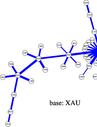
Figure 1: Minimal Spanning Tree with weighted edges for the XAU-based FX network representation calculated for the full interval 12/15/1998-06/30/2008. Line widths are proportional to weights $\omega$ of the corresponding edges, while line lengths are arbitrary.

Figure 1 shows the weighted MST for gold (B $\equiv$ XAU). (Due to the fact that in this and in other MST graphs all the cross-rates share the same base currency, for clarity we denote the nodes only by their price currencies.) Clearly, the network in Figure 1 is dominated by the USD node with the highest degree $K=21$. Other distinguished nodes are SGD ($K=6$), EUR, MAD ($K=5$), and TWD ($K=4$), but none of them can be compared with USD. This supremacy of the USD node over the network is not surprising: according to the Bank of International Settlements 2007 study [9], transactions involving USD account for 86.3% of the global FX turnover, while the same index is 37.0% for euro, 16.5% for yen, and 15.0% for the British pound (both exchange directions were taken into account, thus the numbers for all currencies sum up to 200%). As one can see, despite the above-discussed fact that from a purely economical point of view an MST might at first sight seem to be a rather abstract object, actually its topology can reflect some important properties of the real FX market.

An even more credible topological measure of node centrality in the B-based network is the betweenness $b^{\rm B}({\rm X})$ of a node X, which for an unweighted (binary) MST graph is given by a simple formula:

$$b^{\rm B}({\rm X})=\sum_{{\rm Y,Z}:{\rm Y}\neq{\rm Z}}{\delta^{\rm B}_{\rm Y,Z}({\rm X})\over(N-1)(N-2)},$$ (3)

where $\delta^{\rm B}_{\rm Y,Z}({\rm X})$ equals 1 if the path linking a pair of nodes (Y,Z) goes through X, or equals 0 otherwise. The betweenness thus quantifies a fraction of node pairs that are connected via a node X with respect to the total number of possible pairs (Y,Z) which is equal to $(N-1)(N-2)$. This version of betweenness can be generalized for a weighted MST, but in our case the above-defined topological version is sufficient to characterize the most important properties of the trees. The so-defined betweenness of the main nodes for the XAU-based network has the following values: 0.82 (USD), 0.49 (SGD), 0.37 (MAD), 0.24 (EUR), and 0.17 (TWD). It should be noted, however, that this quantity (together with the node degree $K$) characterizes the structure of the network, while does not necessarily reflect the importance of particular nodes in the global financial system. For example, the XAU/SGD and XAU/MAD cross-rates are rather exotic and their significant role in the MST in Figure 1 stems mainly from their intermediate location between USD and EUR $-$ the actual hubs of the FX market.

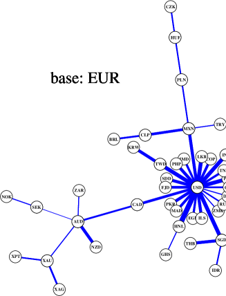
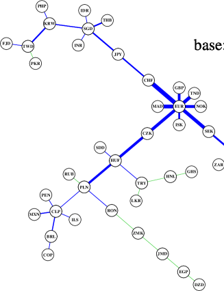
Figure 2: Minimal Spanning Trees for the EUR-based network (top panel) and for the USD-based network (bottom panel) calculated for the full interval 12/15/1998-06/30/2008. Green edges connect anticorrelated nodes.

The MST edges in Figure 1 have widths proportional to their weights. Since almost all the edges are thick, it is straightforward to conclude that the XAU-based network is especially strongly coupled forming a single “supercluster”. However, a finer structure of the XAU-based network, in an agreement with the hierarchical nature [10] of the currency networks, can also be seen: there exists the USD-centered cluster combining the Latin American and Asian currencies, and the EUR-led European cluster joined by MAD and TND. Only the nodes corresponding to XAG and XPT are weakly attached to the rest of MST. This agrees with the obvious observation that the prices of XAU and other precious metals have their own dynamics different from the proper FX market. The narrow edge linking silver and platinum in Figure 1 reflects thus only their residual (secondary) coupling after the primary couplings inside the precious metals group were removed by selecting XAU as the base currency. The geographically driven cluster structure of MST supports the outcomes of the already cited ref. [1, 2, 4].

In a more formal way, clustering properties of a weighted network can be characterized by the average weighted clustering coefficient, describing the average triangle structure of edges [11]:

$$\tilde{C}^{\rm B}=(1/N)\sum_{\rm X}\tilde{c}^{\rm B}({\rm X}),$$ (4)

where $\tilde{c}^{\rm B}({\rm X})$ is defined by

$$\tilde{c}^{\rm B}({\rm X})={1\over K^{\rm B}_{\rm X}(K^{\rm B}_{\rm X}-1)}\sum_{\rm Y,Z}(\tilde{\omega}^{\rm B}_{\rm X,Y}\tilde{\omega}^{\rm B}_{\rm Y,Z}\tilde{\omega}^{\rm B}_{\rm Z,X})^{1/3},$$

$$\tilde{\omega}^{\rm B}_{\rm P,Q}={\omega^{\rm B}_{\rm P,Q}\over\underset{\rm P,Q}{\max}(\omega^{\rm B}_{\rm P,Q})}.$$ (5)

Here $K^{\rm B}_{\rm X}$ is the degree of a node X. Obviously, $\tilde{c}^{\rm B}({\rm X})$ has to be calculated for a complete network, not for its MST representation (which does not comprise any triangles). For the XAU-based network under study the average weighted clustering coefficient is high: $\tilde{C}^{\rm XAU}=0.71$.

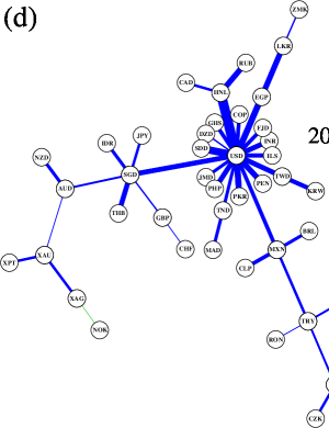
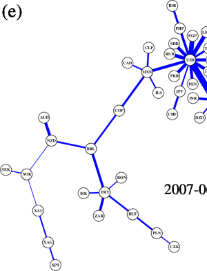
Figure 3: Minimal Spanning Trees for the EUR-based network calculated in subintervals of 2 years (a)-(d) and 1.5 year (e). Green edges connect anticorrelated nodes.

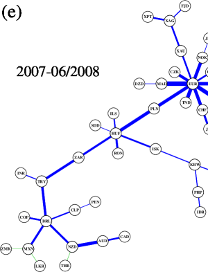
Figure 4: Minimal Spanning Trees for the USD-based network calculated in subintervals of 2 years (a)-(d) and 1.5 year (e). Green edges connect anticorrelated nodes.

Another measure of how compact is the structure of a network is the characteristic path length quantifying the average minimal route between pairs of nodes. For an unweighted (binary) MST graph is given by a simple formula:

$$L^{\rm B}={1\over N(N-1)}\sum_{\rm X,Y:X\neq Y}l^{\rm B}({\rm X,Y}),$$ (6)

where $l^{\rm B}({\rm X,Y})$ denotes the number of edges in a path between nodes X and Y. For the XAU-based MST: $L^{\rm XAU}=1.65$.

The XAU-based network is a representation of the actual FX market as viewed from the perspective of a neutral observer. It therefore reflects only the primary, global structure of the market with two leading nodes: USD and EUR. In order to inspect finer details, we have to eliminate one of these currencies by choosing it as the base currency. The upper panel of Figure 2 shows MST for the EUR-based network and the lower one shows its counterpart for the USD-based network. These two trees have strikingly different topology. The EUR-based MST develops a single cluster of nodes with the USD node (of the degree $K=22$) in its centre. This USD-led cluster comprises currencies of Latin America, Asia, and the Mediterranean region. Disintegration of the EUR-related cluster seen in Figure 1 caused a migration of such nodes as TND and MAD, normally evolving under the influence of euro, to their secondary attractor $-$ USD. Other nodes from that cluster are dispersed more or less randomly over the whole tree and they are connected via edges with small weights. With the topology that apparently resembles ($L^{\rm EUR}=1.53$) the topology of the XAU-based network (Figure 1), the EUR-based network actually has on average evidently smaller edge weights and a smaller clustering coefficient ($\tilde{C}^{\rm EUR}=0.33$).

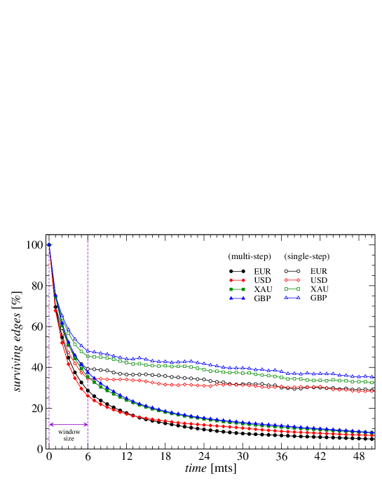
Figure 5: Single-step survival ratio $\sigma^{\rm B}(\delta)$ (open symbols) and multi-step survival ratio $\Sigma^{\rm B}(\delta)$ (full symbols) for 4 representative base currencies: USD (red diamonds), EUR (black circles), GBP (blue triangles), and XAU (green squares). Width of the moving window is denoted by vertical dashed lines.

In contrast to both the XAU-based and the EUR-based minimal spanning trees, the USD-based MST (the lower panel of Figure 2) can be described as being somewhere between a hierarchical and a random graph. There is no central node, the node degree distribution does not have convincing scale-free tails (see ref. [6] for more details), the characteristic path length is long ($L^{\rm USD}=4.10$), and the clustering coefficient is small ($\tilde{C}^{\rm USD}=0.11$). However, despite this small value of $\tilde{C}^{\rm USD}$, a few clusters can be identified in the MST: the European cluster concentrated around EUR, the South and East Asian cluster with SGD as its main hub, the commodity-trade-related cluster around AUD, and the Latin American cluster with the distinguished CLP node. A characteristic feature of this network is the existence of a number of nodes with rather insignificant couplings to the rest of the tree (the thinnest edges in the lower panel of Figure 2). That these edges are distributed almost randomly is suggested by a lack of causal relations between the underlying exchange rates and a lack of considerable economic ties between the corresponding countries. It is noteworthy that due to the US dollar’s dominating role in the global financial system, the currency network based on USD has the finest possible cluster structure of all the network representations of the FX market.

Table 1 summarizes this part of our work, by collecting values of $L^{\rm B}$ and $\tilde{C}^{\rm B}$ for a few exemplary choices of the base currency. All the remaining network representations which are not shown here can be described by the values not exceeding the shown extremes for GHS and USD.

	base: USD	base: GBP	base: EUR	base: MXN	base: CHF	base: AUD	base: PLN	base: JPY	base: XAU	base: GHS
$L^{\rm B}$	4.10	2.33	1.53	2.14	1.63	2.44	1.99	1.95	1.65	1.55
$\tilde{C}^{\rm B}$	0.11	0.31	0.33	0.42	0.43	0.46	0.51	0.51	0.71	0.93

Table 1: Characteristic path length $L^{\rm B}$ and average weighted clustering coefficient $\tilde{C}^{\rm B}$ for a few representative choices of the base currency B calculated for the full period 12/15/1998 $-$ 06/30/2008.

The networks discussed so far and presented graphically in Figures 1 and 2 are in fact only the time-averaged representations of the real currency networks with constantly evolving structure. This evolution can be observed and quantified after increasing temporal resolution of our analysis. Let us split our time series of daily returns into the following subintervals: 1999-2000, 2001-2002, 2003-2004, 2005-2006, and 2007-06/30/2008. For a given base currency we calculate the correlation matrix and the MST graph in each of the subintervals. Figures 3 and 4 show such MSTs for the EUR-based network and the USD-based network, respectively.

	$\tilde{C}^{\rm B}$				$L^{\rm B}$
	base: USD	base: GBP	base: EUR	base: XAU	base: USD	base: GBP	base: EUR	base: XAU
1999-2000	0.08	0.35	0.43	0.72	4.57	1.70	1.21	1.25
2001-2002	0.09	0.29	0.40	0.65	4.53	2.01	1.60	2.30
2003-2004	0.15	0.34	0.32	0.66	3.34	2.62	2.51	2.47
2005-2006	0.19	0.33	0.30	0.83	3.69	2.58	1.99	2.94
2007-2008	0.19	0.37	0.27	0.80	3.68	3.67	2.92	2.67

Table 2: The weighted clustering coefficient $\tilde{C}^{\rm B}$ for the USD-, GBP-, EUR-, and XAU-based networks together with the characteristic path length $L^{\rm B}$ for the corresponding MSTs, calculated in subintervals of 2 years (except the last one which is only 1.5 years long). Note the monotonic trends in $\tilde{C}^{\rm USD}$ and $\tilde{C}^{\rm EUR}$.

The trees in Figures 3 and 4 confirm the significant unstability of the networks, reported already in ref. [3, 4]. However, the observed changes of the structure reveal also some slowly varying components that survive for a few consecutive time intervals. Such a component that can be found in the EUR-based MSTs is a decrease of the USD node degree from $K=24$ in 1999-2000, through $K=18$ in 2001-2002, to $K=13$ over the last 1.5 years (Figure 3). Also in terms of the node betweenness $b^{\rm EUR}$, the USD node gradually loses its centrality: 0.88 (1999-2000), 0.86 (2001-2002), 0.83 (2003-2004), 0.82 (2005-2006), and 0.71 (2007-2008). On the other hand, for the USD-based network the EUR node does not change its degree so dramatically: the degree increased from $K=6$ in 1999-2000 to $K=9$ in 2001-2002 and then it stabilized itself around this value.

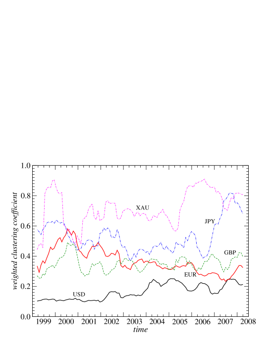
Figure 6: Weighted clustering coefficient $\tilde{C}^{\rm B}$ as a function of time for 5 base currencies: USD (black solid), EUR (red solid), GBP (green dashed), JPY (blue dot-dashed), and XAU (magenta dot-double-dashed).

In order to inspect how these changes affect the average topological properties of the networks, we calculated values of the clustering coefficient $\tilde{C}^{\rm B}$ and of the characteristic path length $L^{\rm B}$ for four base currencies: USD, GBP, EUR and XAU. The results are collected in Table 2. Indeed, for EUR as the base currency the network has gradually become less clustered than it used to be in 1999-2000 ($\tilde{C}^{\rm EUR}$ has dropped from 0.43 to 0.27), while the opposite can be said about the USD-based network ($\tilde{C}^{\rm USD}$ has increased from 0.08 to 0.19). For other choices of B situation is less clear as we cannot identify such explicit trends. Furthermore, we observe that the EUR-based, the GBP-based and the XAU-based MSTs are now more dispersed than they used to be before (a strong increase of $L^{\rm B}$). In contrast, the USD-based tree has become more compact (a noticeable decline of $L^{\rm USD}$ in Table 2).

The existence of monotonic trends in the evolution of the network topology motivated us to track this phenomenon with a higher temporal resolution. We sampled the data with a moving window of length of 6 months (126 trading days) and with a step of one month. As before, for each window position we calculated the corresponding correlation matrices and MSTs. For such short time intervals we expect that the inter-window fluctuations of the network structure are considerably stronger than in the previous case. Therefore we begin with quantitative estimation of the MST temporal stability by means of the single-step survival ratio

$$\sigma^{\rm B}(\delta)={\#\{E^{\rm B}(i)\cap E^{\rm B}(i+\delta)\}\over N-1},$$ (7)

and the multi-step survival ratio [11]

$$\Sigma^{\rm B}(\delta)={\#\{E^{\rm B}(i)\cap E^{\rm B}(i+1)\cap\dots\cap E^{\rm B}(i+\delta)\}\over N-1},$$ (8)

where $E^{\rm B}(i)$ denotes a set of the B-based MST edges for a window $i$. These two ratios tend to overestimate and underestimate, respectively, the number of stable edges in the network [3]. Figure 5 displays the average $\sigma^{\rm B}(\delta)$ and $\Sigma^{\rm B}(\delta)$ expressed in per cent units for different values of time shift $\delta$. It occurs that for disjoint windows ($\delta\geq 6$) the single-step survival ratio is a slowly decaying quantity indicating that, on average, roughly 1/3 of the edges in the initial network exist also after 4 years of evolution. In contrast, only about 5-10% of the edges (i.e. 2-4 edges) remain actually unchanged at least for 4 years. We see that the differences between the networks representing distinct base currencies are small. From Figure 5 one can infer that a vast majority of the edges change their locations with high frequency - as much as 60-75% of the total number of edges, depending on B, do not survive for more than 5 months. These numbers can be compared with the results reported in [3], where the analyzed network of 110 exchange rates between 11 currencies was considerably more stable and about 50% of links were surviving for 2 years. However, the authors of ref. [3] considered only the most liquid major currencies whose mutual relations are more stable than the relations involving less liquid currencies. Moreover, they analyzed data from a distinct time interval characterized by a lack of strong movements of the major cross-rates.

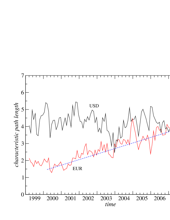
Figure 7: Time dependence of characteristic path length $L^{\rm B}$ for the USD-based (black line) and the EUR-based MST (red line). Dashed line denotes linear trend in $L^{\rm EUR}$.

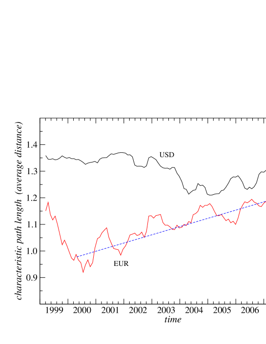
Figure 8: Time dependence of the average internode distance $\mathcal{L}^{\rm B}$ for the USD-based (black line) and the EUR-based fully connected network (red line). Dashed line denotes linear trend in $\mathcal{L}^{\rm EUR}$.

Temporal evolution of the average weighted clustering coefficient for the networks corresponding to USD, EUR, GBP, JPY, and XAU can be seen in Figure 6. The most interesting behaviour is presented by the EUR-based network. After the introduction of euro at the end of 1998, during next 1.5 years $\tilde{C}^{\rm EUR}$ doubled its value from 0.3 to almost 0.6. Then a long process of declining started, which drove the coefficient to its absolute minimum below 0.25 around the middle of 2007. In the first half of 2008 $\tilde{C}^{\rm EUR}=0.33$, i.e. it returned to its initial value. Since the short-time fluctuations of $\tilde{C}^{\rm EUR}$ occur frequently, it is impossible to state whether at present we are witnessing a trend reversal or the latest coefficient increase is only transient, while we are still in the downward trend of $\tilde{C}^{\rm EUR}$. Nevertheless, over past 8 years the currency network viewed from the EUR perspective evolved from a very centralized, USD-oriented network towards a more dispersed, less clustered structure. On the other hand, $\tilde{C}^{\rm USD}$ shows a more balanced behaviour. It started with a value of about 0.1 which was considerably stable for 3 years. Then a period of significant increase of $\tilde{C}^{\rm USD}$ up to 0.2 at the end of 2003 followed, after which no further monotonic trends can be identified. Since the beginning of 2004, $\tilde{C}^{\rm USD}$ has been fluctuating around its average value of 0.2. This means that the USD-based representation of the FX network, in which the EUR node plays a role of the largest hub, has not changed its average structure significantly over past a few years.

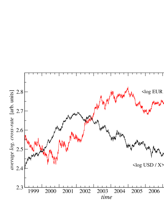
Figure 9: Time dependence of logarithms of USD/X (black) and EUR/X (red) cross-rates averaged over all 45 price currencies X.

Out of three other base currencies from Figure 6, the GBP-based network shows, on average, the highest stability, while both the JPY-based and the XAU-based networks have largely unstable structure. It is interesting that recently the network observed from the JPY perspective has similar clustering coefficient as its XAU-based counterpart. It suggests that the Japanese currency is now strongly decoupled from the rest of currencies and has its own unique evolution. This coincides with a declining role of the Japanese currency in the international currency trade [9].

The above conclusions for USD and EUR receive additional support from Figure 7, where an evolution of the characteristic path lengths is presented for two network representations. As it might be expected based on the outcomes for the clustering coefficient, $L^{\rm EUR}(t)$ displays a clear upward trend (approximated by a dashed line in Figure 7) which has elevated $L^{\rm EUR}$ from about 1.5 in 2000 to about 4 in 2007. Also in agreement with the outcomes reported above, $L^{\rm USD}$ shows only rapid fluctuations around its long-time average, while we do not observe any trend.

These conclusions drawn from Figure 7, based on topological characteristics of the MSTs, can be confirmed by an analogous analysis carried out for the complete networks instead of their MST representations. In order to show this, we have to replace the definition (6) of the characteristic path length $L^{\rm B}$ which, in the case of a fully connected network, would lead to a trivial result. We thus here adopt a definition based on weights rather than topology. According to this, the distance between two nodes is related to their coupling strength: the higher it is, the closer are the nodes. For the network analysed in our work, a good candidate for this measure is the metric distance $d^{\rm B}_{\rm X,Y}$ defined by Eq.(2). Then the average internode distance can be defined by

$$\mathcal{L}^{\rm B}={1\over N(N-1)}\sum_{\rm X,Y:x\neq Y}d^{\rm B}_{\rm X,Y}.$$ (9)

Similar to $d^{\rm B}_{\rm X,Y}$, the above quantity can assume values in the range $0\leq\mathcal{L}^{\rm B}\leq 2$ with a special case of $\mathcal{L}^{\rm B}=\sqrt{2}$ for a set of completely independent exchange rates. In Figure 8 we present temporal evolution of the average internode distance $\mathcal{L}^{\rm B}$ for the USD-based and EUR-based complete networks. We see that over the years $\mathcal{L}^{\rm EUR}$ has evolved according to an increasing linear trend which moved its value from about 0.95 in 2000 to about 1.2 in 2007, in full analogy to what we observe for MSTs in Figure 7. This similarity of behaviour of $L^{\rm B}$ and $\mathcal{L}^{\rm B}$ can be considered an indication that minimal spanning trees constitute a sufficient representation of the forex (or other financial) networks even though this type of graphs might seem to be rather arbitrarily chosen out of a variety of possible other choices.

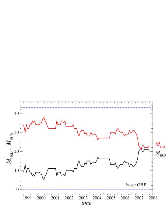
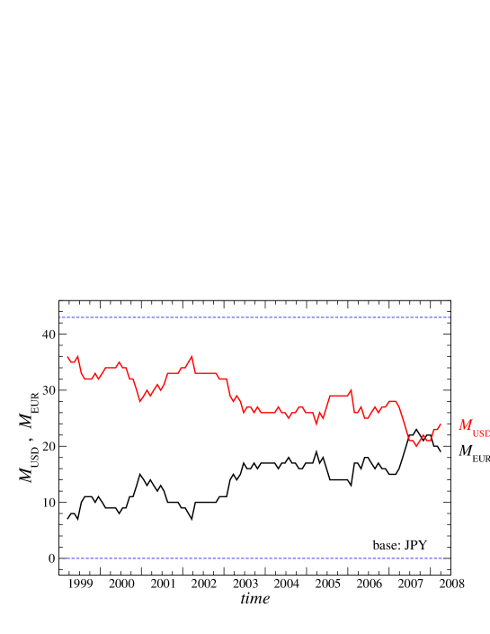
Figure 10: Number $M_{\rm EUR}$ (black) of currencies closer to EUR than to USD in terms of the distance $d^{\rm B}_{\rm X,Y}$ (Eq. (2)) and its complement $M_{\rm USD}$ (red) as functions of time for two representative choices of the base currency: GBP (top) and JPY (bottom).

Now a question emerges, what is the origin of the above-discussed evolution of the FX market. The decrease of the USD node’s centrality, as expressed by a few different quantities, which is visible especially in the EUR-based network since 2000, reflects the fact that now fewer EUR-based cross-rates have a behaviour similar to the behaviour of the EUR/USD cross-rate. This phenomenon can have the following interrelated sources: (i) Some currencies, which originally were satellites of the US dollar (due to, e.g., strong economic dependence of the corresponding countries on the United States), could significantly release their ties and start a more independent evolution. Some of them might even become closer to EUR than to USD, what could explain the increase of the degree of the EUR node seen in Figure 4. (ii) Over the last years a strong depreciation of USD with respect to EUR and other currencies was observed: the EUR/USD cross-rate raised from 0.84 in July 2001 to 1.60 in April 2008. In this context it is worthwhile to look at the average cross-rates of USD and EUR with respect to other currencies shown in Figure 9. Since such a movement did not occur on all EUR-based cross-rates, its occurrence has weakened correlations between EUR/USD and some other EUR-based cross-rates. Thus, in the EUR-based representation of the FX network the USD node can now be less coupled to the rest of the network. This decrease of the USD couplings can also be observed from the perspectives of other currencies as Figure 10 documents. It shows the number of currencies X whose GBP/X (JPY/X) cross-rates were more strongly correlated with GBP/USD (JPY/USD) than with GBP/EUR (JPY/EUR), denoted by $M_{\rm USD}$ (and its complement denoted by $M_{\rm EUR}$). Indeed, $M_{\rm USD}$ considerably declined between 2001 and 2007. Similar observation can be made for a majority of alternative choices of the base currency.

4 Summary

We presented outcomes of our study of the currency network based on daily exchange rates of 46 currencies in the interval from the end of 1998 to the middle of 2008. We showed that the structure of the FX network depends on a choice of the base currency. In the case of currencies which are characterized by an independent, unique dynamics, as precious metals and some exotic currencies, the corresponding network representations have high node-node couplings and are described by high values of the average weighted clustering coefficient. A characteristic property is also almost complete lack of edges with small weights. These networks, if presented in a form of MST, have one dominating node of USD with a high node degree, which is a center of the largest cluster, and a few secondary nodes of a smaller degree. Apart from the USD-led cluster there exists also a significant cluster of European currencies. The USD node’s dominance over the network is even more prominent in the network constructed for EUR and for a few other related currencies. For these currencies, however, due to the disintegration of the European cluster, the corresponding MST has a larger number of edges with small weights, attaching the associated nodes to sometimes random positions. The clustering coefficient assumes medium values in this case. The third type of the FX network representations, with the USD-based network being its representative example, is described by the absence of a dominating node and by high values of the characteristic path length. The EUR node plays here a role of the most notable hub. Among other characteristic features of this representation there are: a clear geographically determined cluster structure, a large number of edges with small weights, and rather small values of the clustering coefficient. All other currency network representations can be located somewhere between the above three poles. It should be recalled, however, that despite these differences between the networks based on different currencies, all of them except the USD-based one have similar scale-free topology in terms of the node degree distribution [6].

The FX network is not stable in time and we showed that its evolution consists of at least two components. The first component is responsible for the rapid and unpredictable fluctuations of the network structure. It comprises both (i) the transient alteration of the cluster structure in which clusters are destroyed while new short-living ones emerge, indicating which currency is in play at the moment, and (ii) the wandering of individual nodes, visible in MSTs, due to random changes in correlation strengths between these nodes and the rest of the network. On the other hand, the second component is represented by slow variations of the network structure and it is responsible for the existence of metastable clusters and long-term trends. This kind of evolution is observed also in ecological networks, where large clusters, even if they build up and exist for a long period of time, in fact strongly fluctuate in size, leaving much freedom for noise (see, e.g., ref. [12]). It is an open question if ecologically-motivated models can well describe properties of the currency market, since there are significant differences (like mutations) and between dynamics of species and currencies. Identifying similarities emerges as an intriguing issue for further study, however.

As our results show, there is a trend in the FX network’s evolution, visible in all the network representations, which was determining the non-random modifications of the network structure for 7 years. It led to a significant decline of the node centrality of USD, as observed from the perpsective of a majority of the base currencies. We identified a possible source of this phenomenon in the strong depreciation of USD value with respect to other leading currencies. There is an additional - in fact related - possibility that the decrease of the USD node’s importance with time and the increasing role of the EUR node, might be due to the fact that euro has become a more influential currency than it used to be in its early years and now more countries consider it as a sufficiently reliable alternative to the US dollar. It will thus be interesting to observe future evolution of the FX network, especially after stabilization of the USD cross-rates to other major currencies.

We finish with a remark on applicability of the minimal spanning trees to analyzing financial data. Despite the fact that MST is only one of many possible graphical representations of the actual network, in our opinion its topology can successfully be studied to collect information on the properties of the complete network. It should be noted that MST, due to the fact that its construction is based on selecting the strongest couplings among network nodes, comprises the core information on the global structure of the network. Thus, the overall characteristics of the network can typicaly also be reproduced in MST. From this point of view, we expect that even if one chose some other type of graph not being a tree, the conclusions based on them would be qualitatively similar to those inferred from the minimal spanning trees. In this context the simplicity of MST makes the application of this graph preferred. Another argument in favour of using MSTs is that results based on them are in satisfactory agreement with knowledge collected from other sources and from intuition.

References

- [1] G.J. Ortega, D. Matesanz, Int. J. Mod. Phys. C 17, 333-341 (2006)
- [2] T. Mizuno, H. Takayasu, M. Takayasu, Physica A 364, 336-342 (2006)
- [3] M. McDonald, O. Suleman, S. Williams, S. Howison, N.F. Johnson, Phys. Rev. E 72, 046106 (2005)
- [4] M.J. Naylor, L.C. Rose, B.J.Moyle, Physica A 382, 199-208 (2007)
- [5] S. Drożdż, A.Z. Górski, J. Kwapień, Eur. Phys. J. B 58, 499-502 (2007)
- [6] A.Z. Górski, S. Drożdż, J. Kwapień, Eur. Phys. J. B 66, 91-96 (2008)
- [7] Sauder School of Business, Pacific Exchange Rate System, http://fx.sauder.ubc.ca/data.html (2008)
- [8] R.N. Mantegna, Eur. Phys. J. B 11, 193-197 (1999)
- [9] Triennial Central Bank Survey on Foreign Exchange and derivatives market activity in 2007 (Bank For International Settlements, 2007)
- [10] E. Ravasz, A.-L. Barabási, Phys. Rev. E 67, 026112 (2003)
- [11] J.P. Onnela, J. Saramaki, J. Kertesz, K. Kaski, Phys. Rev. E 71, 065103 (2005)
- [12] P.E. Anderson, H.J. Jensen, J. Theor. Biol. 232, 551-558 (2005)