Light scattering by an oscillating dipole in a focused beam

Abstract

The interaction between a focused beam and a single classical oscillating dipole or a two-level system located at the focal spot is investigated. In particular, the ratio of the scattered to incident power is studied in terms of the oscillator’s scattering cross section and the effective focal area. Debye diffraction integrals are applied to calculate it and results are reported for a directional dipolar wave. Multipole expansion of the incident beam is then considered and the equivalence between this and the Debye diffraction approach is discussed. Finally, the phase change of the electric field upon the interaction with a single oscillator is studied.

I Introduction

The realization of quantum networks and repeaters for quantum information science crucially depends on an efficient interface between photons and single quantum systems CZH . Strong interaction has been achieved by coupling single emitters to optical resonators BBM ; DPA ; SKF and has also been predicted for emitters located in waveguides where the light is tightly confined in the transverse dimensions KC ; DHR ; SF ; CSD ; ZGL . In free space, the question is to what extent photons may interact with a single oscillating dipole SMK ; PI ; SAL . Recent experiments have demonstrated that light focused on single ions, molecules, or quantum dots may be attenuated in transmission by a few percents GWB ; WGH ; GSD ; VAD ; TCA . In a recent theoretical study we have shown that a focused light beam can be perfectly reflected by a single oscillating dipole located at the focal spot ZNS . In this paper we investigate in more detail the cases where the beam is a focused plane wave and a directional dipole wave. We discuss the equivalence between the multipole expansion and the Debye diffraction approaches. Moreover, we compute the phase shift induced on the electric field by the dipole and find that a few degrees are easily obtainable using realistic focusing parameters and off-resonance excitation.

The strength of the interaction between a beam and an oscillator can be expressed by $\cal K$, the ratio of the scattered to incident power. $\cal K$ can also be given as the ratio of two independent quantities, the scattering cross section $\sigma$ and the inverse of an effective focal area $\cal A$ ZNS ; EK

$${\cal K}=\frac{P_{\rm sca}}{P_{\rm inc}}=\frac{\sigma}{\cal A}~{},$$ (1)

$\sigma$ and $\cal A$ depend exclusively on the oscillator and focusing setup properties, respectively. For a classical oscillator and a two-level system (TLS) the cross section reads

$$\sigma=\left\{\begin{array}[]{ll}\displaystyle\sigma_{0}\frac{{\mathit{\Gamma}}^{2}}{4\Delta^{2}+{\mathit{\Gamma}}^{2}}~{},&\mbox{classical oscillator}\\[5.69054pt] \displaystyle\sigma_{0}\frac{{\mathit{\Gamma}}_{1}^{2}}{4\Delta^{2}+{\mathit{\Gamma}}_{1}^{2}+2{\mathit{\Omega}}^{2}}~{},&\mbox{TLS}~{},\end{array}\right.$$ (4)

where we assumed that there is no damping other than by radiation. $\sigma_{0}=3\lambda^{2}/(2\pi)$ depends solely on the wavelength of the transition Jac . ${\mathit{\Gamma}}$ results from radiation reaction for the classical oscillator Jac , while ${\mathit{\Gamma}}_{1}$ represents the Einstein coefficient of spontaneous decay CDG . $\Delta$ denotes the detuning from resonance and ${\mathit{\Omega}}$ is the Rabi frequency of the TLS, which imposes saturation effects at stronger incident light.

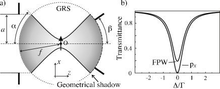
Figure 1: a) The incident light propagating from left to right is focused onto an oscillating dipole located at the focal spot in vacuo. GRS: Gaussian reference sphere, $a$: entrance-aperture radius, $\alpha$: entrance half angle, $\beta$: collection half angle, $f$: focal length, O: focal spot. b) Transmittance as a function of the laser detuning is displayed for a focused plane wave (FPW) with $\alpha=\beta=\pi/3$ and for a directional dipole wave (p_x) with $\alpha=\beta=\pi/2$.

For a point-like oscillator the scattered power depends solely on the field strength at the position of the oscillator. Accounting for the electric nature of the interaction, the effective focal area can be given as the ratio of the power transmitted through the focal plane (FP) and the electric energy density at the focal spot ZNS

$${\cal A}=\frac{\int_{\rm FP}{S}_{z}\,{\rm d}^{2}r}{2cW_{\rm el}({\rm O})}=\frac{\int_{\rm FP}{S}_{z}\,{\rm d}^{2}r}{{S}_{z}({\rm O})}~{},$$ (5)

where $S_{z}$ denotes the $z$ component of the Poynting vector in the FP and $W_{\rm el}({\rm O})$ is the electric energy density at the focal spot O RW . The integration is taken over the FP. The second equality holds for circular symmetry of the incident field strength with respect of the $z$ axis; a condition which, for instance, is obeyed by a focused plane wave (FPW) but not by a directional dipole wave. Figure 1a) describes an ideal lens that projects the incident field onto the Gaussian reference sphere (GRS), which represents the locus of equal phase of the incoming converging and also for the outgoing diverging mode. Because the lens is assumed to be in the far-field region, the fields are tangential on the GRS.

II Debye diffraction

An established approach of calculating the field in the focal area is provided by the Debye diffraction integrals. This approach was initiated by Debye using Green’s theorem Deb and was extended by Wolf using the method of stationary phase Wol . For an incident plane wave the method was extensively applied by Richards and Wolf RW . These considerations led to the Debye diffraction integral for the electric and magnetic fields in the focal area RW ; Sta

$${\bf E}({\bf r})=-\frac{ik}{2\pi}\int_{\Sigma_{\rm inc}}{\bf A}e^{ik{\bf r}\cdot{\bf s}}{\rm d}\Sigma~{},\hskip 56.9055pt{\bf H}({\bf r})=-\frac{ik}{2\pi c}\int_{\Sigma_{\rm inc}}{\bf s}\times{\bf A}e^{ik{\bf r}\cdot{\bf s}}{\rm d}\Sigma~{},$$ (6)

where ${\bf A}$ denotes the vectorial angular spectrum of the incident wave. $k$ is related to the wavelength by $k=2\pi/\lambda$. $\bf r$ is the position in the focal area and ${\bf s}$ is the unit vector in the direction of the plane wave. The integration is carried out over the incident solid angle $\Sigma_{\rm inc}$ bounded by the semiaperture angle $\alpha$. Calculations are presented in Fig. 2 for the case of a directional dipole wave indicated by p_x. Such a wave is constructed by considering the emission pattern at the left hemisphere of the GRS of an electric dipole located at O and oriented along the $x$ axis and by reversing the propagation direction SD . The angular spectra of the FPW RW ; ST1 and the p_x wave read

$${\bf A}=\left\{\begin{array}[]{ll}fE_{0}\sqrt{\cos\theta}\left(\cos\phi\,{\bf e}_{\theta}-\sin\phi\,{\bf e}_{\phi}\right)~{},&\mbox{FPW}\\ fE_{0}\left(\cos\theta\cos\phi\,{\bf e}_{\theta}-\sin\phi\,{\bf e}_{\phi}\right)~{},&{\rm p}_{x}\\ 0~{},&\theta>\alpha~{}.\end{array}\right.$$ (10)

In Figs. 2a) and 2b), the Poynting vector component $S_{z}$ and the electric energy density proportional to $|E_{x}|^{2}$ are displayed along the $x$ and $y$ axes in the FP. Note that the field components $E_{y}$ and $E_{z}$ are zero on these axes. Figure 2c) shows areas of positive and negative values of $S_{z}$ in the FP, i.e. areas of forward and backward propagation. The changes of direction are a signature of field vortices in the focal area, as reported for a FPW Sta ; BDW . In Fig. 2d) the phase of the electric field relative to that of a plane wave is plotted for positions along the $z$ axis. One notes a characteristic phase anomaly in the neighborhood of the focal spot associated with a phase jump of $\pi$, which is also termed Gouy phase BW ; HM . Furthermore there are oscillations, which do not vanish for increasing $z$ displacements. This behavior is singular for propagation along the $z$ axis, while for directions increasingly tilted away from the $z$ axis the oscillations progressively die out at larger distances Deb .

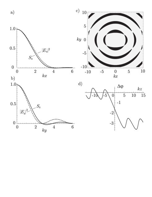
Figure 2: a) The $z$ component of the Poynting vector $S_{z}$ (full curve) and the electric energy density given as $|E_{x}|^{2}$ (dashed curve) of a p_x wave along the $x$ axis in the FP and normalized to their respective values at $x=0$. b) Same as a) but along the $y$ axis. c) Contour plot of $S_{z}$ in the FP. Bright and black areas refer to the Poynting vector in the positive and negative $z$ direction, respectively. d) Phase of the focused electric field $E_{x}$ on the $z$ axis relative to that of a plane wave. Note the oscillatory behavior that does not vanish for large $|z|$-values. $\alpha=\pi/2$ in all cases.

Using Eq. (5) we calculated $\cal A$ for four different cases, namely for the FPW, the p_x wave, the dipolar wave with the generating dipole oriented along $z$ axis, and for combined electric and magnetic generating dipoles directed along the $x$ and $y$ axis, respectively ZNS . Here we present, pars pro toto, the results for the electric field ${\bf E}({\rm O})$ at the origin, the effective focal area $\cal A$, and the scattering ratio $\cal K$ for the p_x wave

$${\bf E}({\rm O})=-i\frac{2kfE_{0}}{3}{\cal F}(\alpha)\,{\bf e}_{x}~{},\hskip 28.45274pt\frac{1}{\cal A}=\frac{k^{2}}{3\pi}{\cal F}(\alpha)~{},\hskip 28.45274pt{\cal K}_{0} = 2{\cal F}(\alpha)~{},$$ (11)

where the subscript of ${\cal K}_{0}$ indicates that $\sigma=\sigma_{0}$ is assumed. The p_x wave has the property that the three quantities depend in the same way on the semiaperture angle $\alpha$ through

$${\cal F}(\alpha)=\frac{1}{4}\left(4-3\cos\alpha-\cos^{3}\alpha\right)~{}.$$ (12)

As pointed out in Ref. ZNS , ${\cal K}_{0}$ reaches for $\alpha=\pi/2$ the maximum possible value of 2, which also establishes the maximum possible scattering ratio for a directional focused beam in free space. ${\cal K}_{0}>1$ indicates that the scattered power is larger than the incident power. However, this does not violate the energy conservation law because of destructive interference in the forward direction. Taking the interference into account the transmittance $\cal T$, the ratio of the transmitted and incident power, is given by

$${\cal T}=1-{\cal R}=1-\frac{1}{2}\frac{\sigma}{\cal A}~{},$$ (13)

where $\cal R$ is the reflectance, the ratio of the back scattered to incident power. The factor of 1/2 in the second equality accounts for the fact that equal amount of scattering takes place in the forward and backward directions. Based on the procedure outlined in Ref. ZNS we also determined the transmittance as a function of the semiaperture angle $\alpha$ and semicollection angle $\beta$

$${\cal T}_{0}(\alpha,\beta)=1-\frac{1}{16}\left(4-3\cos\alpha-\cos^{3}\alpha\right)\left(4+3\cos\left(\max\{\alpha,\beta\}\right)+\cos^{3}\left(\max\{\alpha,\beta\}\right)\right)~{},$$ (14)

where the subscript to ${\cal T}_{0}$ indicates that $\sigma=\sigma_{0}$ is assumed. Examples of $\cal T$ as a function of the detuning are presented in Fig. 1b) for the FPW and for the p_x wave. Figure 3 displays a rapid decrease of ${\cal T}_{0}$ with increasing $\alpha$ and an edge along the geometrical shadow boundary $\alpha=\beta$, as for the FPW ZNS . As shown in Eq. (14), ${\cal T}_{0}$ is invariant with respect to $\beta$ for $\beta<\alpha$, while for $\beta>\alpha$, ${\cal T}_{0}$ increases with $\beta$. Contrary to the FPW, ${\cal T}_{0}(\alpha,\beta)$ decreases monotonously with increasing $\alpha$ and reaches the value of zero at $\alpha=\pi/2$.

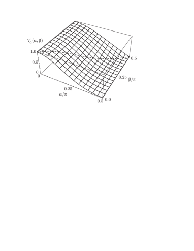
Figure 3: Transmittance ${\cal T}_{0}$ of a p_x wave as a function of the angles $\alpha$ and $\beta$ as defined in Fig. 1a. The dashed curve indicates the edge along the geometrical shadow boundary $\alpha=\beta$.

III Multipole expansion

Another approach convenient for the description of focused fields is given by a multipole expansion ST1 ; Str ; BH ; vEn ; MSA . Adopting the notation of Bohren and Huffman BH we write for the electric field in the most general form

$${\bf E}({\bf r})=\sum\limits_{\ell}\sum\limits_{m=0}^{\ell} \left(B_{e,m,\ell}{\bf M}_{e,m,\ell}({\bf r})+A_{e,m,\ell}{\bf N}_{e,m,\ell}({\bf r})+e\rightarrow o\right)~{},$$ (15)

where ${\bf M}_{{\scriptstyle e\atop\scriptstyle o},m,\ell}({\bf r})$ and ${\bf N}_{{\scriptstyle e\atop\scriptstyle o},m,\ell}({\bf r})$ are real valued and denote complete sets of magnetic and electric multipoles. $B_{{\scriptstyle e\atop\scriptstyle o},m,\ell}$ and $A_{{\scriptstyle e\atop\scriptstyle o},m,\ell}$ are the corresponding coefficients. Assuming a linearly polarized field in front of the incident lens and aligning the $x$ axes to the incident field polarization the expansion in Eq. (15) can be restricted to ${\bf M}_{o,1,\ell}({\bf r})$ and ${\bf N}_{e,1,\ell}({\bf r})$ multipoles for the electric field and to ${\bf M}_{e,1,\ell}({\bf r})$ and ${\bf N}_{o,1,\ell}({\bf r})$ for the magnetic field, respectively.

The calculation of the coefficients requires some attention NRH . The source-free field mode may be considered as a sum of the converging incoming and diverging outgoing field. Because the outgoing mode is purely a consequence of the incoming mode, only the latter is needed for a unique determination of the coefficients. This concept was applied for instance by Sheppard and Török ST1 , where the multipoles of the expansion were associated with spherical Hankel functions. The direct expansion in terms of multipoles for the source-free field is also possible. However, in this case the converging field at the entrance and the diverging field at the exit of the GRS have to be taken into account. For this purpose the field symmetry on the GRS has to be considered Wol1 ; CW , which can be derived from the Debye scattering integrals in Eqs. (6) when assuming positions diametral with respect to the origin

$${\bf E}(-{\bf r}) = -\frac{ik}{2\pi}\int_{\Sigma_{\rm inc}}{\bf A}e^{-ik{\bf r\cdot s}}\,{\rm d}\Sigma=\left[\frac{ik}{2\pi}\int_{\Sigma_{\rm inc}}{\bf A}e^{ik{\bf r\cdot s}}\,{\rm d}\Sigma\right]^{*}=-{\bf E}^{*}({\bf r})~{},$$ (16)

which means that the field is antihermitian for diametral positions on the GRS. The corresponding relationship of the field’s phase $\varphi$ reads

$$\varphi(x,y,z)=-\varphi(-x,-y,-z)-\pi,~{}{\rm mod}~{}2\pi~{}.$$ (17)

The phase shift of $-\pi$ demonstrates the phase anomaly in the neighborhood of the focal spot (see Fig. 2d) and it is equal to the Gouy phase acquired when the beam traverses the focus.

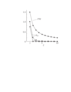
Figure 4: Multipole expansion coefficients for the non-focused plane wave (PW) and the p_x wave. $|A_{e,1,\ell}|/E_{0}=|B_{o,1,\ell}|/E_{0}$ (dots) are presented for the PW and $|A_{e,1,\ell}|/(E_{0}fk)$ (dots) and $|B_{e,1,\ell}|/(E_{0}fk)$ (circles) for the p_x wave, respectively. For the latter a semiaperture angle of $\alpha=\pi/2$ was assumed.

Here we follow the approach of Borghi Bor and Borghi et al. BSA and expand the angular spectrum $\bf A$ of the incident field in surface vector harmonics and substitute the expansion into Eqs. (4). This procedure assures that the Debye-diffraction and multipole-expansion method are literally the same. We write for the expansion

$${\bf A}=\frac{(-i)^{\ell}}{2k}\sum\limits_{\ell=1}^{\infty}\left(B_{o,1,\ell}{\bf\widetilde{M}}_{e,1,\ell}+iA_{e,1,\ell}{\bf\widetilde{N}}_{e,1,\ell}\right)~{},$$ (18)

where ${\bf\widetilde{M}}_{o,m,\ell}(\theta,\phi)$ and ${\bf\widetilde{N}}_{e,m,\ell}(\theta,\phi)$ are real valued and complete sets of vectorial surface harmonics, which are independent on the radial variable $r$. They are related to the spherical vector harmonics ${\bf Y}$ and $\bf Z$ by Jac ; LegendreP

$$\begin{array}[]{lll}{\bf Y}_{\ell}^{1}&=&\displaystyle i\left(\frac{2\ell+1}{2\pi\ell(\ell+1)}\right)^{1/2}\left({\bf\widetilde{M}}_{e,1,\ell}+i\,{\bf\widetilde{M}}_{o,1,\ell}\right)~{},\\[5.69054pt] {\bf Z}_{\ell}^{1}&=&\displaystyle i\left(\frac{2\ell+1}{2\pi\ell(\ell+1)}\right)^{1/2}\left({\bf\widetilde{N}}_{e,1,\ell}+i\,{\bf\widetilde{N}}_{o,1,\ell}\right)~{},\end{array}$$ (21)

where ${\bf Z}_{\ell}^{1}={\bf s}\times{\bf Y}_{\ell}^{1}$. Because of the completeness and orthogonality of the basis functions, the coefficients are given by

$$\begin{array}[]{lll}B_{{\scriptstyle e\atop\scriptstyle o},1,\ell}&=\displaystyle 2ki^{\ell-1}\frac{2\ell+1}{2\pi\ell^{2}(\ell+1)^{2}}\int_{\Sigma_{\rm inc}}{\bf A}\cdot{\bf\widetilde{M}}_{{\scriptstyle e\atop\scriptstyle o},1,\ell}\,{\rm d}\Sigma~{},\\[8.53581pt] A_{{\scriptstyle e\atop\scriptstyle o},1,\ell}&=\displaystyle-2ki^{\ell}\frac{2\ell+1}{2\pi\ell^{2}(\ell+1)^{2}}\int_{\Sigma_{\rm inc}}{\bf A}\cdot{\bf\widetilde{N}}_{{\scriptstyle e\atop\scriptstyle o},1,\ell}\,{\rm d}\Sigma~{},\end{array}$$

where the prefactors result from normalization of the basis functions and from accounting of the Whittaker type of transformation, which provides a relationship between surface vector harmonics and multipoles Whi ; DW . For the magnetic multipoles this relationship reads

$${\bf M}_{{\scriptstyle e\atop\scriptstyle o},1,\ell}({\bf r}) = \frac{(-i)^{\ell}}{4\pi}\int_{4\pi}{\bf\widetilde{M}}_{{\scriptstyle e\atop\scriptstyle o},1,\ell}({\bf s})e^{ik{\bf s}\cdot{\bf r}}{\rm d}\Sigma=j_{\ell}(kr){\bf\widetilde{M}}_{{\scriptstyle e\atop\scriptstyle o},1,\ell}(\theta,\phi)~{},$$ (24)

and analogously for the electric multipoles

$${\bf N}_{{\scriptstyle e\atop\scriptstyle o},1,\ell}({\bf r}) = \frac{1}{k}\nabla\times{\bf M}_{{\scriptstyle e\atop\scriptstyle o},1,\ell}({\bf r})=\frac{(-i)^{\ell-1}}{4\pi}\int_{4\pi}{\bf s}\times{\bf\widetilde{M}}_{{\scriptstyle e\atop\scriptstyle o},1,\ell}({\bf s})e^{ik{\bf s}\cdot{\bf r}}{\rm d}\Sigma=\frac{(-i)^{\ell-1}}{4\pi}\int_{4\pi}{\bf\widetilde{N}}_{{\scriptstyle e\atop\scriptstyle o},1,\ell}({\bf s})e^{ik{\bf s}\cdot{\bf r}}{\rm d}\Sigma~{}.$$ (25)

We finally write the fields in terms of multipoles

$${\bf E}({\bf r}) = \sum\limits_{\ell=1}^{\infty}\left(B_{o,1,\ell}{\bf M}_{o,1,\ell}({\bf r})+A_{e,1,\ell}{\bf N}_{e,1,\ell}({\bf r})\right)~{},$$ (26)

$${\bf H}({\bf r}) = \frac{-i}{c}\sum\limits_{\ell=1}^{\infty}\left(B_{o,1,\ell}{\bf N}_{o,1,\ell}({\bf r})+A_{e,1,\ell}{\bf M}_{e,1,\ell}({\bf r})\right)~{},$$ (27)

and for completeness we also present expressions for the surface vector harmonics and multipoles

$$\widetilde{\bf M}_{{\scriptstyle e\atop\scriptstyle o},1,\ell} = \displaystyle\pi_{\ell}{-\sin\phi\atop~{}\cos\phi}\,{\bf e}_{\theta}-\tau_{\ell}{\cos\phi\atop\sin\phi}\,{\bf e}_{\phi}~{},$$

$$\widetilde{\bf N}_{{\scriptstyle e\atop\scriptstyle o},1,\ell} = \displaystyle\tau_{\ell}{\cos\phi\atop\sin\phi}\,{\bf e}_{\theta}+\pi_{\ell}{-\sin\phi\atop~{}\cos\phi}\,{\bf e}_{\phi}~{},$$

$${\bf M}_{{\scriptstyle e\atop\scriptstyle o},1,\ell} = \displaystyle j_{\ell}\widetilde{\bf M}_{{\scriptstyle e\atop\scriptstyle o},1,\ell}~{},$$

$${\bf N}_{{\scriptstyle e\atop\scriptstyle o},1,\ell} = \displaystyle\frac{1}{kr}\left(\ell(\ell+1)j_{\ell}\pi_{\ell}{\cos\phi\atop\sin\phi}\,{\bf e}_{r}+S_{\ell}\,\widetilde{\bf N}_{{\scriptstyle e\atop\scriptstyle o},1,\ell}\right)~{},$$

where $j_{\ell}=j_{\ell}(kr)$ is the spherical Bessel function. $S_{\ell}$ is a related to $j_{\ell}$, and $\pi_{\ell}$ and $\tau_{\ell}$ follow from the Legendre polynomials $P_{\ell}^{1}$ as

$$S_{\ell}=\frac{{\rm d}(krj_{\ell}(kr))}{{\rm d}(kr)}~{},\hskip 28.45274pt\pi_{\ell}=\frac{P_{\ell}^{1}(\cos\theta)}{\sin\theta}~{},\hskip 28.45274pt\tau_{\ell}=\frac{{\rm d}P_{\ell}^{1}(\cos\theta)}{{\rm d}\theta}~{}.$$ (28)

In Fig. 4 we depict the coefficients $A_{e,1,\ell}$ and $B_{o,1,\ell}$ of the p_x wave for $\alpha=\pi/2$, and compare them with the coefficients of a non-focused plane wave (PW) BH . We note that $A_{e,1,\ell}$ differs from zero for even $\ell$ except for $\ell=1$ while the $B_{o,1,\ell}$ coefficients differ from zero exclusively for odd $\ell$. The fact that coefficients with $\ell>1$ do not vanish for the p_x wave is somewhat surprising. However, these are required to maintain the propagation characteristics of a directional wave and to guarantee power conservation throughout the space on the basis of a source-free focused field. Figure 5 displays the quality of the expansion for the FPW and p_x wave when the number of terms is truncated. It is apparent that quite a few terms are required for a decent reproduction of the angular spectra for $\alpha=\pi/2$ and even more terms are required for $\alpha<\pi/2$.

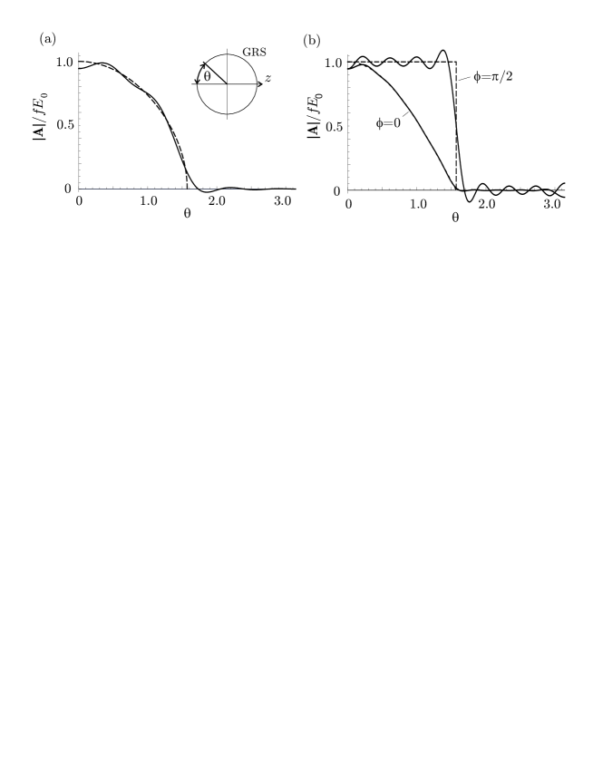
Figure 5: Angular spectra $\bf A$ of the incident field according to Eq. (10) and approximations according to Eq. (18) are given by dashed and full lines, respectively, for $\alpha=\pi/2$. (a) FPW. (b) Dependence along the $x$ and $y$ direction, indicated by $\phi=0$ and $\phi=\pi/2$, respectively, for the p_x wave. The inset indicates the angle $\theta$ as it is considered for this figure. The summation of terms is truncated to $\ell_{\rm max}=8$ and 16 in (a) and (b), respectively.

Of special interest is the property that all multipoles are zero at the origin except the electric dipole mode ${\bf N}_{e,1,1}^{(1)}$. Therefore, in cases where the field at the origin only is relevant, the analysis can be simplified by decomposing the incident field into dipolar and nondipolar modes. This concept was introduced by van Enk vEn and was considered in Refs. PI ; ZNS . ${\bf N}_{e,1,1}$ at the origin and in the far-field region reads BH

$$\begin{array}[]{lll}{\bf N}_{e,1,1}^{(1)}&=\frac{2}{3}{\bf\hat{e}}_{x},&{\bf r}={\rm O}~{},\\[8.53581pt] \displaystyle{\bf N}_{e,1,1}^{(3)}&=\frac{\displaystyle e^{i(kr-\pi/2)}}{kr}\left(\cos\theta\cos\phi\,{\bf\hat{e}}_{\theta}-\sin\phi\,{\bf\hat{e}}_{\phi}\right),&kr\gg 1,~{}z>0~{},\end{array}$$ (31)

where the superscripts (1) and (3) denote the source-free field with the spherical Bessel function and the outgoing mode with the spherical Hankel function, respectively. The concept of field decomposition into dipolar and nondipolar components becomes particularly useful when the scattered field ${\bf E}_{\rm sca}$ is considered, which in the case of a classical dipole oriented along the $x$ axis is given by

$${\bf E}_{\rm sca}({\bf r})=-\frac{3}{2}E_{\rm inc}({\rm O})\frac{{\mathit{\Gamma}}}{2\Delta+i{\mathit{\Gamma}}}\frac{e^{ikr}}{kr}\left(\cos\theta\cos\phi\,{\bf\hat{e}}_{\theta}-\sin\phi\,{\bf\hat{e}}_{\phi}\right),\hskip 28.45274ptkr\gg 1~{}.$$ (32)

Inserting the expression

$$E_{\rm inc}({\rm O})=A_{e,1,1}{\bf N}_{e,1,1}^{(1)}({\rm O})\cdot{\bf e}_{x}~{},$$ (33)

into Eq. (32), it is fairly easy to see that at resonance the dipole component of the incident field is exactly canceled by the scattered field in the forward direction. Therefore, the outgoing field is given by

$${\bf E}_{\rm out}={\bf E}_{\rm inc}+{\bf E}_{\rm sca}={\bf E}_{\rm inc}-A_{e,1,1}\frac{{\mathit{\Gamma}}}{2\Delta+i{\mathit{\Gamma}}}\frac{e^{ikr}}{kr}\left(\cos\theta\cos\phi\,{\bf\hat{e}}_{\theta}-\sin\phi\,{\bf\hat{e}}_{\phi}\right)~{},$$ (34)

where, apart from ${\bf E}_{\rm inc}$, the coefficient $A_{e,1,1}$ is the only variable that depends on the focusing specifications. For the FPW and the p_x wave, $A_{e,1,1}$ is given analytically as

$$A_{e,1,1}=\left\{\begin{array}[]{ll}\displaystyle-i\frac{1}{10}fkE_{0}\left(8-\cos^{3/2}\alpha\left(5+3\cos\alpha\right)\right)~{},&\mbox{FPW}\\[8.53581pt] \displaystyle-i\frac{1}{4}fkE_{0}\left(4-3\cos\alpha-\cos^{3}\alpha\right),&\mbox{ p}_{x}~{}.\end{array}\right.$$ (37)

For a p_x wave with $\alpha=\pi/2$, $A_{e,1,1}/(fkE_{0})=1$ as shown in Fig. 4. Furthermore, by inserting Eqs. (31) and (37) into Eq. (33) one sees that the electric field at the origin is the same as in Eq. (11), confirming that the Debye-diffraction and the multipole-expansion methods yield identical results.

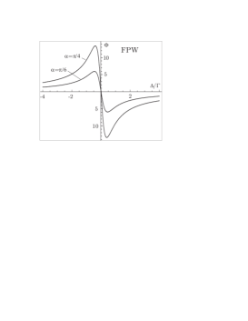
Figure 6: Phase shift $\Phi$ of Eq. (43) in units of degrees as a function of the laser detuning. Results are plotted for the FPW and for two different semiaperture angles $\alpha$, as indicated.

IV Phase shift by scattering

With the above considerations it is also easy to calculate the phase shift $\Phi$ imposed on the beam by a single oscillator at the focal spot. The phase shift $\Phi$ is defined by

$$\Phi={\rm arg}\left({\bf E}_{\rm out}\cdot{\bf E}_{\rm inc}^{*}\right)~{},$$ (38)

where ${\bf E}_{\rm inc}^{*}$ is introduced as a reference field for the detection of the phase shift. Making use of Eqs. (34) and (37) and assuming that a detector is positioned on the $z$ axis, we find

$$\Phi={\rm arg}\left(1-\frac{i{\mathit{\Gamma}}}{2\Delta+i{\mathit{\Gamma}}}~{}\times\begin{array}[]{ll}\frac{1}{10}\left(8-\cos^{3/2}\alpha\left(5+3\cos\alpha\right)\right)\\[5.69054pt] \frac{1}{4}\left(4-3\cos\alpha-\cos^{3}\alpha\right)\end{array}\right)\begin{array}[]{ll},\mbox{ FPW}\\[5.69054pt] ,\mbox{ p}_{x}~{},\end{array}$$ (43)

where an extra negative sign is introduced to account for the Gouy phase shift of $\pi$ imposed on the incident field. $\Phi$ in Fig. 6 shows a typical dispersive of behavior. It amounts to 5-15 degrees at the extremal points for semiaperture angles accessible in experiments. The extremal points are located at approximately $\Delta/{\mathit{\Gamma}}=1/2$ and $\Phi$ decays only slowly with increasing detuning. We expect that integration over a collection solid angle would not change substantially the picture gained from Eq. (43) because of the coinciding phase fronts of the incident and scattered field.

V Conclusions

We studied the scattering of a FPW and a p_x wave by a single oscillator, with emphasis on the equivalence between the Debye diffraction and multipole expansion approaches. We systematically applied the concept of the GRS as the locus of equal phases in the forward and backward direction and paid special attention to the calculation of the multipole expansion coefficients on the basis of source-free fields. We thus derived an analytical expression ${\cal T}_{0}(\alpha,\beta)$ for the transmittance of a p_x wave. We finally demonstrated that a considerable phase shift of a few degrees is imposed on the light beam by a single oscillator at a detuning significantly larger than the linewidth. This property, for instance, might be exploited for the non-resonant detection of single emitters.

References

- (1) Cirac J.I, Zoller P., Kimble H.J, and Mabuchi H., Phys. Rev. Lett. 78, 3221 (1997).
- (2) Boozer A.D., Boca A., Miller R., Northup T.E. Kimble H.J., Phys. Rev. Lett. 98, 193601 (2007).
- (3) Dayan B., Parkins A.S., Aoki T., Ostby E.P., Vahala K.J., and Kimble H.J., Science 319, 1062 (2008).
- (4) Schuster I., Kubanek A., Fuhrmanek A., Puppe T., Pinkse P.W.H., Murr K., and Rempe G., Nature Phys. 4, 382 (2008).
- (5) Kochan P. and Carmichael H.J., Phys. Rev. A 50, 1700 (1994).
- (6) Domokos P., Horak P., and Ritsch H., Phys. Rev. A 65, 033832 (2002).
- (7) Shen J.T. and Fan S., Opt. Lett. 30, 2001 (2005).
- (8) Chang D.E., Sørensen A.S., Demler E.A., and Lukin M.D., Nature Phys. 3, 807 (2007).
- (9) Zhou L., Gong Z.R., Liu Y.-X., Sun C.P., and Nori F., Phys. Rev. Lett. 101, 100501 (2008).
- (10) Sondermann M., Maiwald R., Konermann H., Lindlein N., Peschel U., and Leuchs G., Appl. Phys. B 89, 489 (2007).
- (11) Pinotsi D. and Imamoğlu A., Phys. Rev. Lett. 100, 093603 (2008).
- (12) Stobin’ska M., Alber G., and Leuchs G., preprint, arXiv:0808.1666 (2008).
- (13) Gerhardt I., Wrigge G., Bushev P., Zumofen G., Agio M., Pfab R., and Sandoghdar V., Phys. Rev. Lett. 98, 033601 (2007).
- (14) Wrigge G., Gerhardt I., Hwang J., Zumofen G., and Sandoghdar V., Nature Phys. 4, 60 (2008).
- (15) Gerardot B.D., Seidl S., Dalgarno P.A., Warburton R.J., Kroner M., Karrai K., Badolato A., and Petroff P.M., Appl. Phys. Lett 90, 221106 (2007).
- (16) Vamivakas A.N., Atatüre M., Dreiser J., Yilmaz S.T., Badolato A., Swan A.K., Goldberg B.B., Imamoğlu A., and Ülnü M.S., Nano Lett. 7, 2892 (2007).
- (17) Tey M.K., Chen Z., Aljunid S.A., Chng B., Huber F., Maslennikov G., and Kurtsiefer C., Nature Phys. 4, 924 (2008).
- (18) Zumofen G., Mojarad N.M., Sandoghdar V., and Agio M., Phys. Rev. Lett. 101, 180404 (2008); EPAPS Document No. E-PRLTAO-101-043834, http://www.aip.org/pubservs/epaps.html.
- (19) van Enk S.J. and Kimble H.J., Phys. Rev. A 61, 051802(R) (2000); ibid. 63, 023809 (2001).
- (20) Jackson J.D., Classical Electrodynamics, 2nd edn. (Wiley, New York, 1975).
- (21) Cohen-Tannoudji C., Dupont-Roc J., and Grynberg G., Atom-Photon Interactions, (Wiley, New York, 1992).
- (22) Richards B. and Wolf E., Proc. Roy. Soc. A 253, 358 (1959).
- (23) Debye P., Ann. Phys. Lpz. 30, 755 (1909).
- (24) Wolf E., Proc. Roy. Soc. A 253, 349 (1959).
- (25) Stamnes J.J., Waves in Focal Regions, (Hilger, Bristol, 1986).
- (26) Stamnes J.J. and Dhayalan V., Pure Appl. Opt. 5, 195 (1996).
- (27) Sheppard C.J.R. and Török P., J. Mod. Opt. 44, 803 (1997).
- (28) Boivin A., Dow J., and Wolf E., J. Opt. Soc. Am. 57, 1171 (1967).
- (29) Born M. and Wolf E., Principles of Optics (Pergamon, Oxford, 1975).
- (30) Hwang J. and Moerner W.E., Opt. Comm. 280, 487 (2007).
- (31) Stratton J.A., Electromagnetic Theory, (McGraw-Hill, New York, 1941).
- (32) Bohren C.F. and Huffman D.R., Absorption and Scattering of Light by Small Particles, (Wiley, New York, 1983).
- (33) van Enk S.J., Phys. Rev. A 69, 043813 (2004).
- (34) Mojarad N.M., Sandoghdar V., and Agio M., J. Opt. Soc. Am. B25, 651 (2008).
- (35) Nieminen T.A., Rubinsztein-Dunlop H., and Heckenberg N.R., J. Quant. Spec. & Rad. Transfer 79-80, 1005 (2003).
- (36) Wolf E., J. Opt. Soc. Am.70, 1311 (1980).
- (37) Collet E. and Wolf E., Opt. Lett.5, 264 (1980).
- (38) Borghi R., J. Opt. Soc. Am. A 21, 1805 (2004).
- (39) Borghi R., Santarsiero M., and Alonso M.A., J. Opt. Soc. Am. 22, 1420 (2005).
- (40) Sign convention for the Legendre Polynomials according to Eq. (4.25) in Ref. BH .
- (41) Whittaker E.T., Math. Ann. 57, 333 (1902).
- (42) Devaney A.J. and Wolf E., J. Math. Phys. 15, 234 (1974).