Band terminations in density functional theory.

Abstract

The analysis of the terminating bands has been performed in the relativistic mean field framework. It was shown that nuclear magnetism provides an additional binding to the energies of the specific configuration and this additional binding increases with spin and has its maximum exactly at the terminating state. This suggests that the terminating states can be an interesting probe of the time-odd mean fields provided that other effects can be reliably isolated. Unfortunately, a reliable isolation of these effects is not that simple: many terms of the density functional theories contribute into the energies of the terminating states and the deficiencies in the description of those terms affect the result. The recent suggestion ZSW.05 that the relative energies of the terminating states in the $N\neq Z,\ A\sim 44$ mass region given by $\Delta E$ provide unique and reliable constraints on time-odd mean fields and the strength of spin-orbit interaction in density functional theories has been reanalyzed. The current investigation shows that the $\Delta E$ value is affected also by the relative placement of the states with different orbital angular momentum ${\it l}$, namely, the placement of the $d$ (${\it l}=2$) and $f$ (${\it l}=3$) states. This indicates the dependence of the $\Delta E$ value on the properties of the central potential.

I Introduction

The density functional theory (DFT) in its non-relativistic BHR.03 and relativistic VRAL realizations is a standard tool of modern nuclear structure studies. However, providing global description of atomic nuclei, it still suffers from the fact that many channels of effective interaction are not uniquely defined: this is a reason for a large variety of the DFT parametrizations, the quality of many of which is poorly known. The spin-orbit interaction and the time-odd mean fields are of particular interest in this context, since there are considerable variations for these quantities (see, for example, Refs. DD.95 ; BRRMG.99 ; AR.00 ). The spin-orbit interaction plays a crucial role in the definition of the shell structure of nuclei, and, thus its accurate description is required so that theoretical tools have predictive power for nuclei beyond known regions. The time-odd mean fields (or nuclear magnetism (NM) in the language of the relativistic mean field (RMF) theory KR.90 ) contribute to the single-particle Hamiltonian only in situations where the intrinsic time-reversal symmetry is broken and Kramers degeneracy of time-reversal counterparts of the single-particle levels is removed. The rotating nuclei and odd and odd-odd mass nuclei are typical examples of such situations, see Refs. BHR.03 ; VRAL and references quoted therein.

It was recently suggested in Ref. ZSW.05 that the set of terminating states in the $N\neq Z,\ A\sim 44$ mass region provides unique and reliable constraints on time-odd mean fields and the strength of spin-orbit interaction in Skyrme density functional theory (SDFT), see also Refs. S.07 ; ZS.07 . Later this procedure (called as ’TS-method’ in this manuscript, where ’TS’ refers to ’terminating states’) has been used in the analysis of terminating states in this mass region within the RMF theory BWSMG.06 which is one of the versions of covariant density functional (CDFT) theory VRAL .

The authors of Refs. ZSW.05 ; S.07 ; ZS.07 ; BWSMG.06 claim that the TS-method is free from the drawbacks of standard methods of defining spin-orbit interaction based on measuring the single-particle energies of the spin-orbit partner orbitals in spherical nuclei. As a consequence, it is stated that it allows to define very accurately both isoscalar and isovector channels of spin-orbit interaction ZSW.05 ; BWSMG.06 ; the feature which was impossible in the previously existing methods.

The conclusions obtained within the TS-method are drastically different from the ones previously obtained in the SDFT and RMF frameworks. For example, based on the comparison of the calculated and experimental energies of spin-orbit partner orbitals, it was shown in Ref. BRRMG.99 that the experimental spin-orbit splittings are better reproduced in the RMF approach than in the SDFT (see Fig. 2 in Ref. BRRMG.99 ). On the contrary, the results obtained in Refs. ZSW.05 ; BWSMG.06 within the TS-method show that the SDFT provides better description of spin-orbit splittings than the RMF: it was suggested in Ref. ZSW.05 that only 5% reduction in isoscalar ls strength is needed in the SDFT approach in order to reproduce experimental data. Considering the conflict of these results and the importance of the spin-orbit interaction in nuclei it is necessary to understand to which extent the basis of the suggested TS-method is sound and justified. The goal of the present manuscript is the study of the properties of terminating bands and their terminating states in the RMF framework. In particular, the question of whether all DFT contributions have been correctly accounted in the realization of the TS-method in Refs. ZSW.05 ; BWSMG.06 is addressed is the current manuscript.

The manuscript is organized as follows. Time-odd mean fields in terminating bands are studied in Sect. II. The basis of the TS-method, its realization in self-consistent DFT and in the Nilsson potential are discussed in Sect. III. Sect. IV analyses the contributions of different DFT terms into the relative energies of terminating states in the $A\sim 44$ mass region. The discussion of the energy scale, its connection to the effective mass of the nucleon and their impact on the relative energies of terminating states is presented in Sect. V. Finally, Sect. VI summarizes main conclusions.

II Time-odd mean fields in terminating bands: test case of ²⁰Ne

Previous DFT investigations of the modifications of the moments of inertia KR.93 ; CRMF ; DD.95 ; YM.00 and single-particle properties AR.00 in rotating nuclei caused by the time-odd mean fields (nuclear magnetism) were restricted to the superdeformed (SD) bands. However, these bands are far away from the termination and are characterized by a relatively stable deformation. In order to understand how NM affects the properties of the terminating bands, the ground state configuration in ²⁰Ne has been studied. This band is a classical example of band termination CNS . It has the $\pi(d_{5/2})^{2}_{4}\nu(d_{5/2})^{2}_{4}$ configuration relative to the ¹⁶O core with maximum spin $I_{max}=8^{+}$. The selection of this configuration has been guided by its simplicity, which allows us to understand the role of time-odd mean fields in terminating bands in greater details. Although the terminating bands were observed also in heavier nuclei, it is difficult to trace them from low spin up to band termination in the self-consistent approaches VRAL without special techniques such as used in the cranked Nilsson-Strutinsky (CNS) approach CNS .

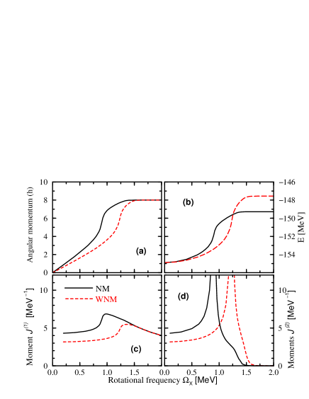
Figure 1: (Color online) Calculated total angular momentum (panel (a)), total binding energy (panel (b)), kinematic and dynamic moments of inertia (panels (c) and (d)) as a function of rotational frequency $\Omega_{x}$ in the ground state band of ²⁰Ne. The results obtained with and without nuclear magnetism are presented. Note that the band termination takes place at rotational frequency above which the subsequent increase of rotational frequency does not modify neither total angular momentum nor total binding energy. This point also corresponds to $\gamma=60^{\circ}$ (Fig. 3c).

The investigation of NM in ²⁰Ne has been carried out within the framework of the cranked relativistic mean field (CRMF) theory KR.89 ; CRMF following the formalism of Ref. AR.00 , where similar study has been performed for the yrast SD band in ¹⁵²Dy. In the CRMF calculations of this manuscript, all fermionic and bosonic states belonging to the shells up to $N_{F}=12$ and $N_{B}=16$ are taken into account in the diagonalization of the Dirac equation and the matrix inversion of the Klein-Gordon equation, respectively. The detailed investigation indicates that this truncation scheme provides very good numerical accuracy. The NL1 NL1 parametrization of the RMF Lagrangian is employed in the study of ²⁰Ne, while the studies of terminating states in the $A\sim 44$ mass region (Sects. III and IV) are performed mostly with the NL1 and NL3 NL3 parametrizations. The pairing is neglected in calculations.

Fig. 1 shows the total angular momentum, total binding energy $E$ and kinematic (J⁽¹⁾) and dynamic (J⁽²⁾) moments of inertia of the ground state configuration in ²⁰Ne as a function of rotational frequency obtained in the calculations with and without NM (the later will be further denoted as WNM). The band crossing caused by the interaction of the $r=+i$ signatures of the [220]1/2 and [211]3/2 orbitals both in the proton and neutron subsystems takes place at lower frequency in the calculations with NM; this is in line with previous finding that the NM shifts the band crossing frequencies AFR.02 . The NM also increases the moments of inertia before band crossing (Fig. 1c,d); similar effect has been seen before in the SD bands (see Ref. AR.00 and references therein). It also leads to a faster alignment of angular momentum with rotational frequency (Fig. 1a); full alignment at $I_{max}=8^{+}$ corresponding to band termination takes place at lower frequency in the calculations with NM.

In the context of study of terminating states two results are important. First, at the band termination the NM does not modify neither total angular momentum (Fig. 1a) nor the expectation values of the single-particle angular momenta $<j_{x}>_{i}$ (Fig. 2). At lower frequency, the impact of NM on $<j_{x}>_{i}$ is similar to the one previously studied in the SD band of ¹⁵²Dy AR.00 , and, thus, it will not be discussed in detail. However, one should mention that when analyzing the impact of NM on $<j_{x}>_{i}$, the region of band crossing and the region close to the band termination have to be excluded from consideration because considerable differences in the deformations of the NM and WNM solutions at given frequency distort their comparison. Second, the NM provides an additional binding to the energies of the specific configuration and this additional binding increases with spin and has its maximum exactly at the terminating state (Fig. 1b and 3d)). This suggests that the terminating states can be an interesting probe of the time-odd mean fields provided that other effects can be reliably isolated.

When the results of the NM and WNM calculations are compared as a function of total angular momentum, one can see that the quadrupole deformation $\beta_{2}$ (Fig. 3a), mass hexadecapole moment $Q_{40}$ (Fig. 3b), and $\gamma$-deformation (Fig. 3c) are almost the same in both calculations. The only difference is seen in the total binding energies (Fig. 3d), where the NM solution is more bound than the WNM solution. These results give a hint why the cranked models based on the phenomenological potentials like Woods-Saxon or Nilsson, which do not include time-odd mean fields DD.95 , are so successful in the description of experimental data. When considered as a function of spin the deformation properties of the rotating system are only weakly affected by the time-odd mean fields, and the proper renormalization of the moments of inertia CNS takes care of the $E$ versus angular momentum curve.

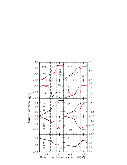
Figure 2: (Color online) The expectation values of single-particle angular momenta $<j_{x}>_{i}$ of the neutron orbitals occupied at low frequency in the ground state configuration of ²⁰Ne given along the deformation path of this configuration. The single-particle orbitals are labeled by means of the asymptotic quantum numbers $[Nn_{z}\Lambda]\Omega$ (Nilsson quantum numbers) of their dominant component of the wave function at $\Omega_{x}=0.0$ MeV. The orbitals with signature $r=+i$ and $r=-i$ are shown in right and left panels, respectively. The results of the calculations with and without NM are shown by solid and dashed lines, respectively. The region of the band crossing is located between the dashed lines.

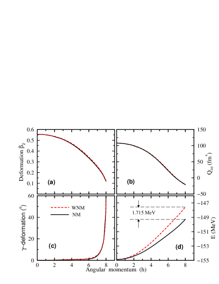
Figure 3: Calculated quadrupole deformation $\beta_{2}$ (panel (a)), mass hexadecapole moment $Q_{40}$ (panel (b)), $\gamma$-deformation (panel (c)), and total binding energy $E$ (panel (d)) as a function of angular momentum. The results obtained with (NM) and without (WNM) nuclear magnetism are presented.

III The TS-method

The TS-method suggested in Ref. ZSW.05 employs the terminating states in the $A\sim 44$ mass region with the proton $d_{3/2}^{-1}\,f_{7/2}^{n+1}$ and $f_{7/2}^{n}$ structure, but, in general, according to Ref. ZS.07 can be employed to terminating states in any mass region. The difference $\Delta E^{exp}=E(d_{3/2}^{-1}\,f_{7/2}^{n+1})-E(f_{7/2}^{n})$ between the excitation energies $E(d_{3/2}^{-1}\,f_{7/2}^{n+1})$ and $E(f_{7/2}^{n})$ of the terminating states with the structure $d_{3/2}^{-1}\,f_{7/2}^{n+1}$ and $f_{7/2}^{n}$ is dominated by the size of the magic gap 20 which is surrounded by the $d_{3/2}$ and $f_{7/2}$ spherical subshells (see Fig. 4).

III.1 The spin-orbit splittings in the TS-method

The principal difference between the standard and the TS-methods of defining the strength of spin-orbit interaction is schematically shown in Fig. 4. The standard method requires that both partners of spin-orbit ${\it ls}$ doublet with $\it j=l\pm\frac{1}{2}$ are observed in experiment since the spin-orbit splitting $\Delta E^{SO}$ is related to the strength of spin-orbit interaction. This severely restricts the possibilities to study spin-orbit interaction since both partners should be located in the vicinity of the Fermi level to be observed: this condition is very difficult to satisfy for high-$j$ orbitals since they are characterized by large spin-orbit splittings, see, for example, Refs. BRRMG.99 ; IEMSF.02 . On the contrary, the TS-method employs the terminating states based on the particle-hole excitations involving the single-particle states with $\it j=l-\frac{1}{2}$ and $\it j^{\prime}=l^{\prime}+\frac{1}{2}$ which emerge from different $N$-shells and are characterized by the energy splitting $\Delta E^{TS}$ (Fig. 4). Since these states are located in the vicinity of the Fermi level, the TS-method provides also information on the spin-orbit interaction of high-$j$ orbitals according to Ref. ZSW.05 .

It is necessary to recognize that both methods of defining the spin-orbit interaction are not free from important drawbacks. The experimental single-particle states in spherical nuclei used in the standard method are strongly affected by the couplings with vibrations in many cases MBBD.85 . On the other hand, the $\Delta E^{TS}$ value used in the TS-method depends not only on the spin-orbit splitting but also on how well the positions of the single-particle states with different orbital momenta $l$ and $l^{\prime}$ (Fig. 4) are described in the DFT calculations. The later fact has been neglected in Ref. ZSW.05 using an analogy with the Nilsson potential, the validity of which is questioned below.

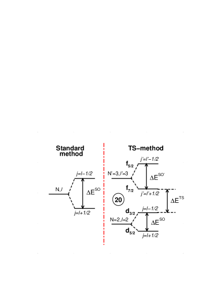
Figure 4: Schematic comparison of the standard and TS-methods of defining the strength of spin-orbit interaction. In the left and right panels, the single-particle spectra without (on left) and with (on right) spin-orbit interaction are compared.

III.2 The TS-method in self-consistent approaches

In the self-consistent calculations, the $\Delta E^{SC}=E(d_{3/2}^{-1}\,f_{7/2}^{n+1})-E(f_{7/2}^{n})$ quantity is defined as the difference of the binding energies of the corresponding terminating states. Without going into the details of specific DFT (nonrelativistic or relativistic), one can conclude that $\Delta E^{SC}$ depends on

• the energy scale of the single-particle spectra which is related to the effective mass $m^{*}(k_{F})/m$ of the nucleon at the Fermi surface,

• the spin-orbit interaction,

• the relative placement of states with different angular momentum $l$,

• the time-odd mean fields (see Sects. II and IV.2),

• the polarization effects (both in time-even and time-odd channels) on going from the $f_{7/2}^{n}$ to the $d_{3/2}^{-1}\,f_{7/2}^{n+1}$ terminating state.

For simplicity of discussion, they will occasionally be called as ’ingredients of $\Delta E^{SC}$’.

$\Delta E^{SC}$ can also be split into the terms which depend on time-even (TE) and time-odd (TO) mean fields

$$\Delta E^{SC}=\Delta E^{SC}_{TE}-\Delta E^{SC}_{TO}$$ (1)

The minus sign in front of $\Delta E^{SC}_{TO}$ reflects the fact that NM always decreases the size of $\Delta E$.

III.2.1 Coupling constant dependence of $\Delta E^{SC}$

The ingredients of $\Delta E^{SC}$ depend in a complicated way on different terms of the DFT with at least one term contributing into each of four first ingredients of $\Delta E^{SC}$ within the nonrelativistic SDFT. In the RMF theory, the spin-orbit interaction is defined in a natural way without additional coupling constant VRAL . The time-odd mean fields related to NM are defined through the Lorentz covariance VRAL and also do not require an additional coupling constant. However, both these terms depend in an indirect way on the coupling constants of other terms of the RMF Lagrangian.

Considering the uncertainties of the description of the ’ingredients of $\Delta E^{SC}$’ in the DFT, it is not obvious that simple fit (to experimental $\Delta E^{exp}$ values) of the coupling constants of the DFT terms related to a pair of ingredients of $\Delta E^{SC}$ (such as time-odd mean fields and spin-orbit interaction as in Ref. ZSW.05 ; the later treated perturbatively) will allow to define these constants in a unique way. This is especially true considering that physical observables depend on many (or sometimes all) coupling constants simultaneously within the DFT, and the effect of varying one or two coupling constants may be either enhanced or cancelled by a variation of others. Strictly speaking, the quality of such perturbative fits involving only one or two terms of the DFT is not known until the results of global fit including all the DFT terms are available. For example, it was shown in Ref. LBBDM.07 that perturbative studies of tensor terms allow only very limited conclusions.

III.2.2 Polarization effects

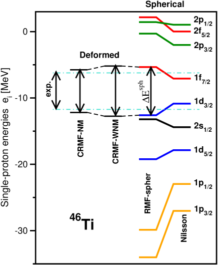
Figure 5: (Color online) (right part) Single-particle energies at spherical shape in ⁴⁶Ti obtained in the RMF calculations with the NL1 parametrization and the Nilsson potential with standard set of parameters BR.85 (columns indicated as “RMF-spher” and “Nilsson”). In order to facilitate the comparison, the RMF states are given at the calculated energies, while the energies of the states obtained in the Nilsson potential are shifted in such a way that the average energy of the $1f_{7/2}$ and $1d_{3/2}$ states is the same in both calculations. (left part) The magnitudes $\Delta E$ of the $f_{7/2}-d_{3/2}$ splittings as extracted from the energies of terminating states ($\Delta E=E(d_{3/2}^{-1}\,f_{7/2}^{n+1})-E(f_{7/2}^{n})$) are shown by arrows in columns “exp” (experiment), “CRMF-NM” and “CRMF-WNM” (CRMF calculations with and without NM). The middle points of arrows are located at the average energy of the $1f_{7/2}$ and $1d_{3/2}$ RMF states. The terminating states are deformed in the CRMF calculations. Note that the value of $\Delta E=5.1$ MeV (not shown in figure) obtained in the cranked Nilsson-Strutinsky calculations compares favorably with experiment ($\Delta E^{exp}=5.51$ MeV).

Fig. 5 illustrates the polarization effects present in the CRMF calculations of terminating states. Since fully stretched states with spin $I_{max}$ are reasonably well described by a single Slater determinant ZSNSZ.07 , the comparison with experiment is performed without angular momentum restoration as in all DFT studies of the terminating $I_{max}$ states in this mass region, see, for example, Refs. ZSW.05 ; BWSMG.06 . At spherical shape, the $f_{7/2}-d_{3/2}$ energy gap ($\Delta E^{sph}$) in the single-particle spectra considerably exceeds $\Delta E^{exp}$. The $\Delta E^{sph}$ value is a very good approximation to the results of the spherical RMF calculations without NM in which the gap between these states is defined as the difference of the binding energies of the $d_{3/2}^{-1}\,f_{7/2}^{n+1}$ and $f_{7/2}^{n}$ states: the difference between two results for all nuclei under study does not exceed 40 keV. When deformation polarization effects denoted as $\Delta E^{def-pol}$ are taken into account (the “CRMF-WNM” column in Fig. 5), this gap becomes even larger and reaches $\Delta E=7.57$ MeV exceeding by 37% the experimental value. The inclusion of NM decreases the difference between experiment and calculations considerably (by 1.14 MeV) (column “CRMF-NM” in Fig. 5). Note that mass and charge quadrupole and hexadecapole moments change only by $\sim 10^{-4}\%$ on going from the CRMF-WNM to CRMF-NM solutions. Thus, the deformation differences between these two solutions are almost non-existant and can be neglected. Based on the consideration of polarization effects, the $\Delta E^{SC}$ can be approximated as

$$\Delta E^{SC}\approx\Delta E^{sph}+\Delta E^{def-pol}-\Delta E^{SC}_{TO}$$ (2)

Considering that the terminating states of interest are close to spherical (Fig. 6), this approximation which corresponds to a perturbative treatment of the deformation polarization effects should be quite reasonable. This approximation also allows to use the results of spherical RMF calculations in subsequent analysis of $\Delta E$ (Sect. IV).

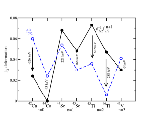
Figure 6: (Color online) Quadrupole deformations of the terminating states obtained in the CRMF calculations with the NL1 parametrization. For each nucleus, the deformation polarization energies $\Delta E^{def-pol}$ are shown between the calculated deformation points. Three nuclei with the largest $\Delta E^{def-pol}$ values are indicated by arrows.

III.3 The Nilsson potential analogy of Ref. ZSW.05

In order to overcome the problems discussed in Sect. III.2.1, the authors of Ref. ZSW.05 use the analogy with the simple form of the Nilsson potential N.55 for the $\Delta E^{SC}_{TE}$ part. This form of the Nilsson potential is similar to the one given below (Eq. (5)), but with the parameters $\kappa$ and $\mu$ independent on principal quantum number $N$. However, no proof (analogy is not a proof) is provided whether such a transition from self-consistent DFT to the Nilsson potential is valid and whether the dependence of the energies of the single-particle states on quantum numbers $N,j,l,$ and $s$ is the same in the self-consistent DFT and in the Nilsson potential. Fig. 5 clearly shows that the later is not a case.

In the simple form of the Nilsson potential, the magnitude of the $f_{7/2}-d_{3/2}$ splitting related to the magic gap 20 is given by

$$\Delta E^{Nil}=\hbar\omega_{0}(1-6\kappa-2\kappa\mu).$$ (3)

Thus, it depends on three major factors: (i) the energy scale of the single-particle potential characterized by $\hbar\omega_{0}$, (ii) the flat-bottom and surface properties entering through the orbit-orbit term $\sim\mu$, and (iii) the strength of the spin-orbit term $\kappa$. Then, the authors of Ref. ZSW.05 using the fact that in light nuclei the Nilsson potential resembles the pure harmonic oscillator potential, which leads to $\mu\sim 0$, conclude that the magnitude of the $f_{7/2}-d_{3/2}$ splitting is given by

$$\Delta E^{Nil}=\hbar\omega_{0}(1-6\kappa).$$ (4)

Thus, in this approximation, the $\Delta E^{Nil}$ splitting is defined only by the energy scale $\hbar\omega_{0}$ and the strength of the $\it{ls}$-potential. Arguing that the energy scale is rather well constrained by the data not only for the Nilsson but also for the self-consistent approaches, the authors of Ref. ZSW.05 conclude that the $f_{7/2}-d_{3/2}$ splitting is directly related to the strength of the $\it{ls}$-potential. Or alternatively, this approximation corresponds to the situation when the $\Delta E^{Nils}$ does not depend on orbital motion of the nucleons.

III.4 An alternative form of the Nilsson potential

One question of paramount importance we have to ask is whether the simple form of the Nilsson potential given in Ref. N.55 and used in Ref. ZSW.05 is unique and how well it describes the experimental data. It turns out that the modern versions of the Nilsson potential employ the parameters $\kappa$ and $\mu$ which are dependent on the main oscillator quantum number $N$ and on nucleon type (proton or neutron), thus facilitating the study of wide range of nuclei with the same set of single-particle parameters and with comparable accuracy BR.85 ; Ragbook ; Rag-priv . Since the Nilsson potential is phenomenological in nature, this procedure is well justified. The accuracy of the description of different physical quantities such as, for example, rotational properties and relative energies of different single-particle configurations BR.85 ; Ragbook ; CNS ; GBI.86 is considerably improved when different values of $\kappa$ and $\mu$ are used for different $N$-shells. Although some variations between the parametrizations exist, this approach is used in almost all parametrizations of the Nilsson potential developed from the middle of the 80ties of the last century GBI.86 ; BR.85 ; A150 . The studies employing this description of the Nilsson potential are abundant and provide systematic information on the accuracy of the description of physical observables in different mass regions. Even more sophisticated dependence of the $\kappa$ and $\mu$ parameters on the principal quantum number $N$ and orbital angular momentum $l$ is introduced in Ref. S.86 and employed in a number of studies, see, for example, Refs. PRet.97 ; BZ.95 .

III.4.1 Terminating states in the $A\sim 44$ mass region

In the Nilsson potential with $\kappa_{N}$ and $\mu_{N}$ parameters dependent on the principal oscillator quantum number $N$ BR.85 ; Ragbook

$$\hat{H}^{Nil-N-dep}-\frac{3}{2}\hbar\omega_{0}=$$ (5)

$$= \hbar\omega_{0}\{N-\kappa_{N}[2{\bm{l}}{\bm{s}}+\mu_{N}(\bm{l}^{2}-<\bm{l}^{2}>_{N})]\},$$

the magnitude of the $f_{7/2}-d_{3/2}$ splitting related to the energy difference of the $d_{3/2}^{-1}\,f_{7/2}^{n+1}$ and $f_{7/2}^{n}$ terminating states is given by

$$\Delta E^{Nil-N-dep}=$$

$$= \hbar\omega_{0}(1-3[\kappa_{2}+\kappa_{3}]-3\kappa_{3}\mu_{3}-\kappa_{2}\mu_{2}).$$

The superscript ${}^{\prime}Nil-N-dep^{\prime}$ is used to indicate the dependence of these expressions on the main oscillator quantum number $N$.

Table 1: The standard parametrization of the Nilsson potential from Ref. BR.85 ; Ragbook . Only the parameters for the $N=2$ and 3 shells are shown.

	Protons		Neutrons
N	$\kappa$	$\mu$	$\kappa$	$\mu$
2	0.105	0.00	0.105	0.00
3	0.090	0.30	0.090	0.25

The $\kappa_{N}$ and $\mu_{N}$ parameters of the so-called standard parametrization of the Nilsson potential are shown for the shells of interest in Table 1. For the protons, the value $\Delta E^{Nil-N-dep}=0.415\hbar\omega_{0}$ is obtained in the calculations employing the $\kappa_{N}$ parameters from the Table 1 but assuming the $\mu_{N}=0$ as it was done in the derivation of Eq. (4). This value can be compared with the $\Delta E^{Nil-N-dep}=0.334\hbar\omega_{0}$ value obtained with the $\kappa_{N},\mu_{N}$ parameters from the Table 1. One can see that these two values differ by approximately 25% and this difference is solely attributed to the non-zero value of the $\mu_{3}$ parameter. Considering that $\Delta E^{exp}\sim 5.5$ MeV (see Fig. 7), 25% difference correspond to 1.4 MeV; this difference definetely cannot be ignored when experimental data is compared with experiment.

III.4.2 Concluding remarks

Even for terminating states in the $A\sim 44$ mass region one cannot ignore the dependence of the energies of the (N,l) and (N’,l’) states, from which the ${\it j=l-\frac{1}{2}}$ and ${\it j^{\prime}=l^{\prime}+\frac{1}{2}}$ states used in the TS-method emerge (see Fig. 4), on the orbital angular momentum. This dependence enters through the $\mu_{N}(\bm{l}^{2}-<\bm{l}^{2}>_{N})]$ term of the Nilsson potential (Eq. (5)). This is contrary to the approximation made in the derivation of Eq. (4) which has a consequence that the energy difference $\Delta E^{Nils}$ depends only on the energy scale $\hbar\omega_{0}$ and the strength of the spin-orbit term $\kappa$. The dependence of $\Delta E^{Nils}$ on the orbital angular momentum in the case of terminating states involving single-particle states from higher $N$-shells has been recognized in Ref. ZS.07 .

IV Terminating states in the $A\sim 44$ mass region: what we can learn from the comparison with experiment

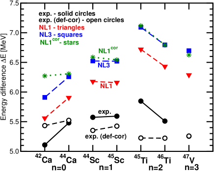
Figure 7: (Color online) The experimental and calculated magnitudes $\Delta E$ of the $f_{7/2}-d_{3/2}$ splittings as extracted from the energies of terminating states ($\Delta E=E(d_{3/2}^{-1}\,f_{7/2}^{n+1})-E(f_{7/2}^{n})$). The results of the CRMF calculations are shown for the NL1 and NL3 parametrizations of the RMF Lagrangian. The experimental data corrected for the deformation polarization effects (as obtained in the NL1 parametrization) is shown by open circles. Note that the experimental and deformation polarization corrected values of $\Delta E$ coincide in the case of ⁴⁷V.

Fig. 7 compares the results of calculations with experiment. The same data set as in Refs. ZSW.05 ; BWSMG.06 is used in this comparison, but it is shown as a function of $n$, where $n$ stands for the number of the $f_{7/2}$ protons in the $f_{7/2}^{n}$ terminating state. In addition, this figure compares the absolute values and not the differences between experimental results and calculations as it was done in Refs. ZSW.05 ; BWSMG.06 : the differences normalized to ⁴⁴Ca are compared in Fig. 8a. Since the $n$ value is the same for each isotope chain ($n=0$ for the Ca isotopes, $n=1$ for the Cs isotopes, $n=2$ for the Ti isotopes, and $n=3$ for the V isotopes), the isospin dependence of $\Delta E$ is clearly visible. Different isotope chains show different isospin dependencies and they are well reproduced in the calculations (Fig. 7 and Fig. 8a). On the other hand, the calculations overestimate the absolute value of $\Delta E$ (Fig. 7), and the difference between the calculated and experimental $\Delta E$ values show pronounced $n$-dependence (Fig. 8a).

One source of the discrepancy between theory and experiment is related to the impact of effective mass of the nucleon on the single-particle spectra (see Sect. V): in general, it should lead to an overestimate of experimental $\Delta E$ in the calculations. The other sources of these discrepancies are analyzed in detail in this Section.

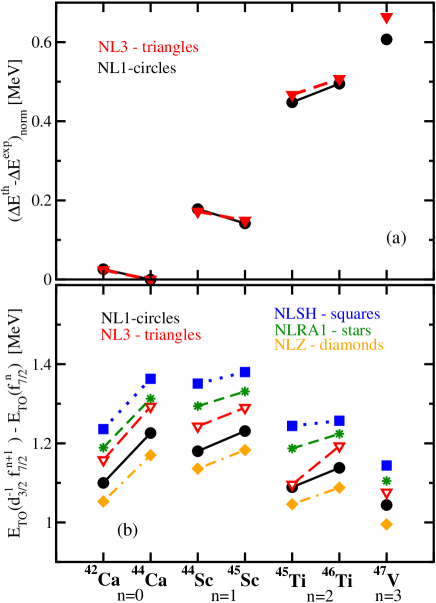
Figure 8: (Color online) (a) The difference $(\Delta E^{th}-\Delta E^{exp})_{norm}$ between the calculated and experimental values of $\Delta E$ (based on the results of Fig. 7). This difference is normalized to zero for ⁴⁴Ca. (b) The calculated difference $E_{TO}(d_{3/2}^{-1}\,f_{7/2}^{n+1})-E_{TO}(f_{7/2}^{n})$ shown as a function of $n$ for the indicated RMF parametrizations (based on the results of Fig. 9).

IV.1 Deformation polarization effects

The deformation polarization effects discussed in Sect. III.2.2 are characterized by the $\Delta E^{def-pol}$ energies. The sign of $\Delta E^{def-pol}$ depends on relative deformations of the $f_{7/2}^{n}$ and $d_{3/2}^{-1}f_{7/2}^{n+1}$ terminating states (Fig. 6). It is positive (negative) when the $\beta_{2}$-deformation of the $d_{3/2}^{-1}f_{7/2}^{n+1}$ state is larger (smaller) than the one of the $f_{7/2}^{n}$ state. The $\Delta E^{def-pol}$ values almost do not depend on the parametrization of the RMF Lagrangian: the difference in their values is below 10 keV if the results of the NL1 and NL3 parametrizations are compared. If the experimental data are corrected for these deformation polarization effects, then smooth trend (the curve ’exp. (def-cor)’ in Fig. 7) as a function of $n$ emerges. The $\Delta E$ value along this curve decreases by $\sim 0.25$ MeV on going from $n=0$ to $n=3$. Assuming that these effects are reasonably well described in the calculations, one can conclude that the nucleus-dependent fluctuations in experimental value of $\Delta E$ (the curve ’exp.’ in Fig. 7) are due to deformation polarization effects.

IV.2 Nuclear magnetism (time-odd mean fields) in the terminating states of the $A\sim 44$ mass region

Fig. 9 shows the additional bindings $E_{TO}(state)$ to the energies of terminating states due to NM. This quantity increases with the increase of the $n$-value for the $f_{7/2}^{n}$ and $d_{3/2}^{-1}\,f_{7/2}^{n+1}$ terminating states. The increase of $E_{TO}$ with isospin within specific isotope chain is associated with the increase of the number of the occupied neutron $f_{7/2}$ states and corresponding increase in spin. The increase of the values of $E_{TO}$ correlates with the increase of the spin of the terminating states: for example, the $f_{7/2}^{n}$ and $d_{3/2}^{-1}\,f_{7/2}^{n+1}$ terminating states have $I_{max}=6^{+}$ and $I_{max}=11^{-}$ in ⁴²Ca and $I_{max}=\frac{31}{2}^{-}$ and $I_{max}=\frac{35}{2}^{+}$ in ⁴⁷V, respectively.

The results of the calculations confirm previous conclusion obtained in ²⁰Ne (Sect. II) that the additional binding due to NM is considerably enhanced in the terminating states. At no rotation, the additional binding due to NM to the energies of the single-particle configurations in odd-mass nuclei is in average around $\sim 100$ keV and seldom reaches 200 keV in the mass region of interest AA.08 . This is much smaller than the additional binding observed in the terminating states in which it reaches 4 MeV for $n=3$ (Fig.  9).

Because of their magnitude, the $E_{TO}$ values in terminating states are also a good measure of how well the time-odd mean fields are defined in the specific version of DFT. The $E_{TO}$ values obtained with different frequently used non-linear parametrizations of the RMF Lagrangian such as NL1 NL1 , NL3 NL3 , NLSH NLSH , NLRA1 NLRA1 and NLZ NLZ are shown in Fig. 9. With increasing $E_{TO}$ and $n$, the absolute variations in the $E_{TO}$ values calculated with different RMF parametrizations increase. However, they are still within 15% of the absolute value of $E_{TO}$. This result suggests that within the non-linear versions of the RMF Lagrangian NM is defined with similar accuracy.

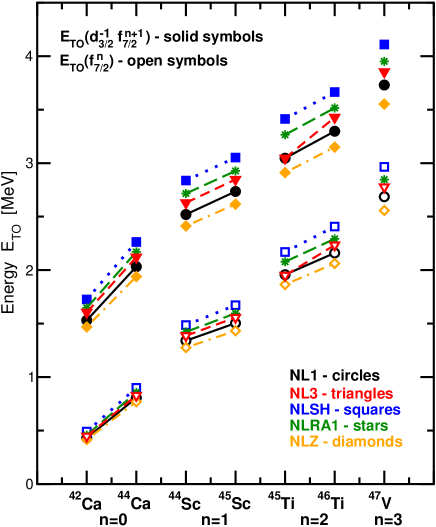
Figure 9: (Color online) Additional bindings $E_{TO}(state)$ (in absolute value) to the energies of terminating states due to NM shown for the terminating states of interest. The results are shown for the indicated parametrizations of the RMF Lagrangian as a function of $n$.

This value can be used to estimate the uncertainty in the definition of the moments of inertia in the CRMF calculations due to the uncertainty in NM. Dependent on the nuclear system, the NM contribution to the total kinematic moment of inertia is approximately 10-25% CRMF ; AA.08 . Thus, the uncertainty of the definition of the absolute value of the total kinematic moments of inertia due to the uncertainty in the definition of NM is modest being in range of 1.5-3.75%.

It follows from Fig. 8 that the portion of the $n$-independent part of the discrepancy between experimental and calculated $\Delta E$ values may be related to the uncertainties in NM since the difference $E_{TO}(d_{3/2}^{-1}\,f_{7/2}^{n+1})-E_{TO}(f_{7/2}^{n})$ somewhat (within $\approx 200$ keV) depends on the RMF parametrization. The contribution of NM into the $n$-dependent part of this discrepancy is discussed in Sect. IV.3.3.

IV.3 The dependence of $\Delta E$ on orbital angular momentum and spin-orbit interaction

IV.3.1 The impact of density modifications on the single-particle properties

It is well known fact that the modifications of the central nucleonic potential and its surface properties affect the single-particle states with different angular momentum l in a different way (see Refs. MBBD.85 ; RBRMG.98 and references therein). They also alter the spin-orbit potential and lead to the changes in the spin-orbit splittings. In order to check how big this effect is in the nuclei under study, the proton density distributions and single-particle spectra at spherical shape are compared in Fig. 10 for the ⁴²Ca and ⁴⁷V nuclei. These nuclei represent the lower and upper mass ends of the data set under investigation. The configuration of ⁴⁷V has 2 additional $f_{7/2}$ neutrons and 3 additional $f_{7/2}$ protons as compared with the configuration of ⁴²Ca. The filling of these high-$j$ orbitals increases the density near the surface (Fig. 10a). These modifications of the density change the central and spin-orbit nucleonic potentials (in a similar fashion as it was discussed in Refs. TPC.04 ; AF.05 ) leading to the modifications of the single-particle spectra (Fig. 10b).

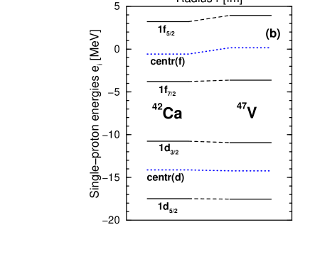
Figure 10: (Color online) (a) Proton density distribution in the ⁴²Ca and ⁴⁷V nuclei as obtained for ground state in the spherical RMF calculations with the NL1 parametrization of the Lagrangian. (b) Corresponding energies of the single-particle states. The states in ⁴²Ca are shown at the calculated energies, while all states in ⁴⁷V are shifted by constant value in such a way that the average energy of the $1d_{3/2}$ and $1f_{7/2}$ states is the same as in ⁴²Ca.

On going from ⁴²Ca to ⁴⁷V, the spin-orbit splitting in the $d_{5/2}-d_{3/2}$ doublet decreases by 0.12 MeV (from 6.72 MeV to 6.60 MeV), while the one in the $f_{7/2}-f_{5/2}$ doublet increases by 0.57 MeV (from 7.0 MeV to 7.57 MeV). If the modifications in the single-particle spectra would be restricted only to the spin-orbit splittings and their modifications would evenly be redistributed between the $j=l+1/2$ and $j=l-1/2$ members of the spin-orbit doublet, this would decrease the $1f_{7/2}-1d_{3/2}$ splitting by 0.22 MeV.

However, the calculations show that the $f_{7/2}-d_{3/2}$ splitting is increased by 0.34 MeV (Figs. 10). Assuming that the energy scale does not change on going from ⁴²Ca to ⁴⁷V, this can only be explained by the change of the relative positions of the $d$ (${\it l}=2$) and $f$ (${\it l}=3$) states from which the $d_{3/2}$ and $f_{7/2}$ states emerge. Unfortunately, there is no straightforward way in the RMF calculations to get an access to the $(N,l)$ states (in sense of Fig. 4). Thus, in order to illustrate the dependence on l, the centroid energy (denoted as “centr(state)” in Fig. 10b) and defined as an average energy of the members of spin-orbit doublet is used. Fig. 10b shows that the energy gap between the centroids of the $d$ and $f$ spin-orbit doublets increases by 0.55 MeV on going from ⁴²Ca to ⁴⁷V. As a consequence of this increase and the above discussed changes in the spin-orbit splittings, the $1f_{7/2}-1d_{3/2}$ splitting increases by 0.34 MeV. This value represents more than half of the increase of $(\Delta E^{th}-\Delta E^{exp})_{norm}$ on going from ⁴²Ca to ⁴⁷V (Fig. 8a).

IV.3.2 Relative placements of the states with different angular momentum $l$

The fact that the relative placement of states with different orbital angular momentum $l$ (especially, of high-$l$ states) is not well reproduced in non-relativistic and relativistic mean field models is well known, see Refs. MBBD.85 ; RBRMG.98 ; LBBDM.07 . The origin of this problem is connected with the surface profile of the mean field and kinetic terms. Microscopic considerations indicate that the effective mass of the nucleon has a pronounced surface profile which is insufficiently parametrized in the present mean field models MBBD.85 . In Refs. ZSW.05 ; BWSMG.06 , this fact has been ignored and no proof has been provided that the placement of the $d$ and $f$ states, from which the $d_{3/2}$ and $f_{7/2}$ states, emerge is correct.

It turns out that the difference in absolute value of $\Delta E$ obtained in the NL1 and NL3 parametrizations (Fig. 8) is well explained by the differences in the relative energies of the $d$ and $f$ states in these parametrizations. The energy gap between the centroids of the $d$ and $f$ spin-orbit doublets is larger in the NL3 parametrization as compared with the NL1 one by approximately 400 keV. If one corrects the NL1 results by this energy gap, one gets the results indicated as NL1^cor in Fig. 7. The NL1^cor results are very close to the NL3 ones, which strongly suggests that the difference between the NL1 and NL3 results is predominantly due to different relative energies of the $l=3$ and $l=2$ states in these parametrizations of the RMF Lagrangian.

Ref. BWSMG.06 has attributed the fact that the NL1 and NL3 parametrizations differ in the description of the absolute $\Delta E$ value (Fig. 7) to the magnitude of the iso-scalar spin-orbit potential. The current investigation does not support this interpretation.

These results suggest that instead of readjusting the isoscalar strength of the spin-orbit interaction as it was done in Ref. ZSW.05 , one can attempt to readjust the coupling constants of the DFT terms influencing the relative energies of the $l=2$ and $l=3$ states with the same effect on $\Delta E$. Indeed, 5% reduction of the isoscalar strength of the spin-orbit interaction introduced in Ref. ZSW.05 reduces $\Delta E$ by $\sim 350$ keV and this change in $\Delta E$ almost does not depend on nucleus (Fig. in Ref. SW.08 ). On the other hand, the CRMF results suggests that the same effect can be achieved if the relative distance of the $d$ and $f$ states is modified. Indeed, the $\Delta E$ values obtained in the CRMF calculations decrease by approximately the same amount on going from the NL3 to NL1 parametrization of the RMF Lagrangian and this decrease only weakly depends on the nucleus (Fig. 7).

IV.3.3 The $n$-dependence of $(\Delta E^{th}-\Delta E^{exp})_{norm}$

The $(\Delta E^{th}-\Delta E^{exp})_{norm}$ quantity shows pronounced dependence on $n$ (Fig. 8a) and its trend (if normalized to a single nucleus) almost does not depend on the RMF parametrization. In order to understand which ingredients of $\Delta E^{SC}$ contribute into this $n$-dependence, the variations $\delta E_{i}=\Delta E_{i}(nucleus)-\Delta E_{i}(^{47}V)$ of different ($i$-th) terms contributing to $\Delta E^{SC}$ are studied below. Contrary to Fig. 8a, ⁴⁷V is selected as a reference in order to get a picture less disturbed by large fluctuations of some variations in the vicinity of ⁴²Ca (Fig. 11). The $\delta E_{TO}=\delta(E_{TO}(d_{3/2}^{-1}\,f_{7/2}^{n+1})-E_{TO}(f_{7/2}^{n}))$ variation is obtained in the deformed CRMF calculations (from Fig. 8b), while other variations shown in Fig. 11 are calculated in spherical RMF calculations. Thus, I effectively employ the approximation given in Eq. (2) assuming that the deformation polarization effects are the same both in theory and experiment. All the results presented here are based on the calculations with the NL1 parametrization, but it was checked that the NL3 results are similar.

The $\delta((\Delta E^{th}-\Delta E^{exp})_{norm})$ variation indicates that the difference between the calculated and experimental $\Delta E$ values decreases with decreasing $n$. Note that for a given $n$ it is almost constant indicating only weak isospin dependence of this variation. The largest changes as a function of nucleus amongst the calculated variations are seen in the energy gap between the centroids of the $d$ and $f$ spin-orbit doublets (the curve denoted as “$\delta E({\it l}-{\rm centroids})$” in Fig. 11). It has the same trend as $\delta((\Delta E^{th}-\Delta E^{exp})_{norm})$ as a function of $n$. For a given $n$, it shows very large dependence on isospin. The second largest variation is seen in the spin-orbit splitting of the $f_{7/2}-f_{5/2}$ spin-orbit doublet (the curve denoted as “$\delta E_{\it ls}(f_{7/2}-f_{5/2})/2$” in Fig. 11). The factor 1/2 is used in this variation since only one half of the total variation of spin-orbit splitting contributes into the $f_{7/2}-d_{3/2}$ splitting (see Sect. IV.3.1). The $\delta E_{\it ls}(f_{7/2}-f_{5/2})/2$ variation has the wrong trend as compared with $\delta((\Delta E^{th}-\Delta E^{exp})_{norm})$. The $\delta E_{\it ls}(d_{5/2}-d_{3/2})/2$ variation of the spin-orbit splitting in the $d_{5/2}-d_{3/2}$ doublet is quite small. It has the correct trend as compared with $\delta((\Delta E^{th}-\Delta E^{exp})_{norm})$.

The $\delta E(f_{7/2}-d_{3/2})$ variation of the $f_{7/2}-d_{3/2}$ splitting approximately satisfies the relation

$$\delta E(f_{7/2}-d_{3/2})=\delta E({\it l}-{\rm centroids})+$$

$$\delta E_{\it ls}(f_{7/2}-f_{5/2})/2+\delta E_{\it ls}(d_{5/2}-d_{3/2})/2$$ (7)

The isospin dependencies seen in $\delta E({\it l}-{\rm centroids})$ and $\delta E_{\it ls}(f_{7/2}-f_{5/2})/2$ act is opposite directions, thus, reducing the isospin dependence of $\delta E(f_{7/2}-d_{3/2})$ as compared with the one of $\delta E({\it l}-{\rm centroids})$. However, the $\delta E(f_{7/2}-d_{3/2})$ variation (Sect. IV.3.1) cannot completely account neither for absolute value nor for isospin dependence (for a given $n$) of the $\delta((\Delta E^{th}-\Delta E^{exp})_{norm})$ variation.

Only when the $\delta E(f_{7/2}-d_{3/2})$ variation is combined with the $\delta E_{TO}$ variation due to NM by

$$\delta E^{sum}=\delta E(f_{7/2}-d_{3/2})+\delta E_{TO}$$ (8)

a better description of the $\delta((\Delta E^{th}-\Delta E^{exp})_{norm})$ variation emerges. For a given $n$, the isospin dependence of the $\delta((\Delta E^{th}-\Delta E^{exp})_{norm})$ is well described by $\delta E^{sum}$. The absolute value of $\delta((\Delta E^{th}-\Delta E^{exp})_{norm})$ for the Ti nuclei is well described by $\delta E^{sum}$. However, for the Ca and Sc nuclei, the difference between these two quantities reaches $30\%$ of the absolute value of $\delta((\Delta E^{th}-\Delta E^{exp})_{norm})$. The part of this discrepancy is definitely related to the limitations of the approximation given by Eq. (2).

Thus, the current study clearly shows that the modifications of the relative placement of the states with different angular momentum $l$, the spin-orbit splittings and time-odd mean fields on going from ⁴⁷V to ⁴²Ca contribute into the $n$-dependence of the difference between the calculated and experimental $\Delta E$ values (the $\Delta E^{th}-\Delta E^{exp})_{norm}$ quantity). Previously, this $n$-dependence of $(\Delta E^{th}-\Delta E^{exp})_{norm}$, expressed in a different form (Fig. 1 in Ref. BWSMG.06 , has been solely attributed to the deficiency of the iso-vector term of the spin-orbit interaction BWSMG.06 , but the current investigation does not support such an interpretation.

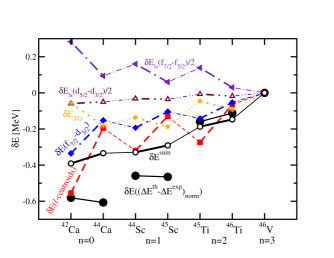
Figure 11: (Color online) The variations $\delta E_{i}$ of different terms contributing to the $\delta(\Delta E^{th}-\Delta E^{exp})_{norm})$ variation, see text for detail.

V The energy scale and the effective mass of the nucleon

The terminating states are expected to be of predominantly single-particle nature CNS ; ZSNSZ.07 : the $d_{3/2}^{-1}\,f_{7/2}^{n+1}$ terminating states are obtained from the $f_{7/2}^{n}$ terminating state by particle-hole (p-h) excitation from the $d_{3/2}$ state into the $f_{7/2}$ state. The energy of this p-h excitation depends on the energies of above mentioned states, and, thus, it is affected by the energy scale of the single-particle spectra which is related to the effective mass $m^{*}(k_{F})/m$ of the nucleon at the Fermi surface.

In the RMF theory, the spin-orbit interaction is effectively scaled by the effective mass of the nucleon (Ref. R.89 ), and that is a reason why experimental data on spin-orbit splittings are well described in the calculations RBRMG.98 ; BRRMG.99 . This scaling also explains why the spin-orbit splittings of the $1p_{3/2}-1p_{1/2}$, $1d_{5/2}-1d_{3/2}$ and $1f_{7/2}-1f_{5/2}$ spin-orbit partner orbitals are almost the same in the RMF and the Nilsson potential calculations (Fig. 5). Note, that the Nilsson potential is characterized by the effective mass $m^{*}(k_{F})/m\sim 1$ which is typical for experimental density of the quasiparticle states. Only in the case of the $2p_{3/2}-2p_{1/2}$ doublet, the spin-orbit splitting is smaller in the RMF calculations.

On the other hand, the energies of the centroids of the spin-orbit doublets are stretched out in the RMF calculations as compared with the Nilsson potential: the difference between the RMF and Nilsson centroid energies increases on going away from the Fermi level (Fig. 5). Thus, the stretching out of the single-particle spectra due to low effective mass of the nucleon shows up mostly for orbital motion of particles and affects the relative placement of the levels with different angular momentum l. The origin of this problem has been discussed in Sect. IV.3.2.

The effective mass of nucleon at the Fermi surface (Lorentz mass in the notation of Ref. JM.89 for the case of the RMF theory) is $m^{*}(k_{F})/m\sim 0.65$ in the RMF theory BRRMG.99 , $\sim 0.7$ in the case of the Hartree-Fock (HF) approach based on the Gogny forces BHR.03 , and varies in the range $0.6-1.0$ in the HF approach based on the Skyrme forces BHR.03 revealing much larger flexibility of this type of the DFT with respect of effective mass. As a consequence of low effective mass, the calculated spectra are less dense than the experimental ones: the well known fact in non-relativistic and relativistic models both for spherical MBBD.85 ; LR.06 ; RBRMG.98 and deformed systems A250 ; BBDH.03 . This study shows that the $\Delta E^{SC}$ quantity differs from the $f_{7/2}-d_{3/2}$ energy gap in the spherical single-particle spectra only by the effects of time-odd mean fields and deformation polarization effects (Sect. III.2.2). These facts pose an open problem on how to compare the experimental data on $\Delta E$ with the results of the DFT calculations (especially, those with low effective mass) since the experimental data on $\Delta E^{exp}$ is expected to be characterized by $m^{*}(k_{F})/m\sim 1$. The implicit assumption used in Refs. ZSW.05 ; BWSMG.06 that the DFT reproduces the empirical $\Delta E$ values relatively well, say within $\sim 10\%$ SW.08 , may be too optimistic especially for the DFT with low effective mass.

VI Conclusions

In conclusion, the following results were obtained in the study of band termination within the DFT framework:

• At band termination, the NM does not modify neither total angular momentum nor the expectation values of the single-particle angular momenta $<j_{x}>_{i}$ of the single-particle orbitals. NM provides an additional binding to the energies of the specific configuration and this additional binding increases with spin and has its maximum exactly at the terminating state. This suggests that the terminating states can be an interesting probe of the time-odd mean fields related to NM provided that other effects can be reliably isolated.

• The realization of the TS-method in Refs. ZSW.05 ; BWSMG.06 is based on the analogy with simple form of the Nilsson potential which allows to neglect the deficiences in the relative placement of the states with different angular momentum $l$. This approximation is not valid for terminating states in the $A\sim 44$ mass region in modern and most frequently used versions of the Nilsson potential

• The impact of the relative placement of the states with different angular momentum $l$ on $\Delta E^{SC}$ is also clearly visible in the RMF calculations. The difference in absolute $\Delta E^{SC}$ values obtained in the CRMF calculations with the NL1 and NL3 parametrizations of the Lagrangian is defined by the different relative energies of the $l=3$ and $l=2$ states in these parametrizations. The modifications of the relative distance of the states with different angular momentum $l$ on going from ⁴⁷V to ⁴²Ca contribute into the $n$-dependence of the difference between the calculated and experimental $\Delta E$ values (the $\Delta E^{th}-\Delta E^{exp})_{norm}$ quantity) in addition to the ones due to the spin-orbit interaction and time-odd mean fields.

The detailed analysis of the TS-method in the RMF framework reveals the picture which is more complicated than the one suggested in Refs. ZSW.05 ; BWSMG.06 . The relative placement of the states with different angular momentum ${\it l}$, defined by the properties of central potential, has to be taken into account in addition to the DFT terms discussed in these references when the $\Delta E$ quantity is analyzed. Considering the similarities of the RMF theory and SDFT, it is very likely that these conclusions are also valid in the SDFT framework. The current investigation calls for a detailed study of the impact of the relative placement of the states with different orbital angular momentum ${\it l}$ on the $\Delta E^{SC}$ quantity in the SDFT framework.

Existing results for superdeformed bands in ³²S MDD.00 ; Pingst-A30-60 and low-spin states in odd mass nuclei AA.08 point to the time-odd mean fields as a major point of the difference between SDFT and RMF. For example, the additional binding due to time-odd mean fields and the energy separation between different signatures of the SD bands are considerable stronger in SDFT as compared with RMF MDD.00 . The current study clearly shows that the correlations induced by time-odd mean fields are large: additional binding due to NM reaches 4 MeV for $n=3$ (Fig. 9), which is by order of magnitude larger than those seen before in the RMF calculations at low spin. It also has a considerable impact on $\Delta E^{SC}$: $\Delta E_{TO}\sim 1.2$ MeV (Fig. 8b). These results call for a comparative study of time-odd mean fields in the Skyrme DFT and RMF frameworks. Such study is necessary in order to make a significant progress towards a better understanding of the role of time-odd mean fields. The work in this direction is in progress and the results will be presented in a forthcoming manuscript AA.08 .

VII Acknowledgements

The material is based upon work supported by the Department of Energy under Award Number DE-FG02-07ER41459.

References

- (1) H. Zdunczuk, W. Satula, and R. A. Wyss, Phys. Rev. C71, 024305 (2005).
- (2) M. Bender, P.-H. Heenen, and P.-G. Reinhard, Rev. Mod. Phys. 75, 121 (2003).
- (3) D. Vretenar, A. V. Afanasjev, G. A. Lalazissis, and P. Ring, Phys. Rep. 409, 101 (2005).
- (4) J. Dobaczewski and J. Dudek, Phys. Rev. C52, 1827 (1995).
- (5) M. Bender, K. Rutz, P.-G. Reinhard, J. A. Maruhn, and W. Greiner, Phys. Rev. C60, 034304 (1999).
- (6) A. V. Afanasjev and P. Ring, Phys. Rev. C62, 031302(R) (2000).
- (7) W. Koepf and P. Ring, Nucl. Phys. A511, 279 (1989).
- (8) W. Satula, Int. J. Mod. Phys. E, v.16, No.2, 360 (2007).
- (9) M. Zalewski and W. Satula, Int. J. Mod. Phys. E, v.16, No.2, 386 (2007).
- (10) A. Bhagwat, R. Wyss, W. Satula, J. Meng, and Y. K. Gambhir, reprint nucl-th/0605009.
- (11) J. König, and P. Ring, Phys. Rev. Lett. 71, 3079 (1993).
- (12) A. V. Afanasjev, J. König and P. Ring, Nucl. Phys. A608, 107 (1996).
- (13) M. Yamagami and K. Matsuyanagi, Nucl. Phys. 672, 123 (2000).
- (14) A. V. Afanasjev, D. B. Fossan, G. J. Lane and I. Ragnarsson, Phys. Rep. 322, 1 (1999).
- (15) W. Koepf and P. Ring, Nucl. Phys. A493, 61 (1989).
- (16) P.-G. Reinhard, et al, Z. Phys. A323, 13 (1986).
- (17) G. A. Lalazissis, J. König and P. Ring, Phys. Rev. C 55, 540 (1997).
- (18) A. V. Afanasjev, S. G. Frauendorf, and P. Ring, Proc. Int. Conf. “The nuclear many-body problem 2001”, Kluwer Academic Publishers, 2002, Eds. W. Nazarewicz and D. Vretenar, p. 103.
- (19) V. I. Isakov, K. Erokhina, H. Mach, M. Sanchez-Vega, and B. Fogelberg, Eur. Phys. J. A14, 29 (2202).
- (20) C. Mahaux, P. F. Bortignon, R. A. Broglia, and C. H. Dasso, Phys. Rep. 120, 1 (1985).
- (21) T. Lesinski, M. Bender, K. Bennaceur, T. Duguet, and J. Meyer, Phys. Rev. C 76, 014312 (2007).
- (22) T. Bengtsson and I. Ragnarsson, Nucl. Phys. A436, 14 (1985).
- (23) M. Zalewski, W. Satula, W. Nazarewicz, G. Stoitcheva, and H. Zdunczuk, Phys. Rev. C 75, 054306 (2007).
- (24) S. G. Nilsson, Dan. Mat.-Fys. Medd. 29, 1 (1955).
- (25) S. G. Nilsson and I. Ragnarsson, Shapes and Shells in Nuclear Structure, Cambridge University Press, 1995.
- (26) I. Ragnarsson, private communication, 2007.
- (27) D. Galeriu, D. Bucurescu, and M. Ivaşku, J. Phys. G 12, 329 (1986).
- (28) T. Bengtsson, Nucl. Phys. A513, 124 (1990).
- (29) T. Seo, Z. Phys. A324, 43 (1986).
- (30) K. Pomorski, P. Ring, G. A. Lalazissis, A. Baran, Z. Lojewski, B. Nerlo-Pomorska, and M. Warda, Nucl. Phys. A624, 349 (1997).
- (31) B. Nerlo-Pomorska and B. Mach, At. Data Nucl. Data Tables 60, 287 (1995).
- (32) A. V. Afanasjev and H. Abusara, in preparation.
- (33) M. M. Sharma, M. A. Nagarajan, and P. Ring, Phys. Lett. B312, 377 (1993).
- (34) M. Rashdan, Phys. Rev. C 63, 044303 (2001).
- (35) M. Rufa, P.-G. Reinhard, J. A. Maruhn, W. Greiner, M. R. Strayer, Phys. Rev. C 38, 390 (1988).
- (36) K. Rutz, M. Bender, P.-G. Reinhard, J. A. Maruhn, and W. Greiner, Nucl. Phys. A634, 67 (1998).
- (37) B. G. Todd-Rutel, J. Piekarewicz, and P. D. Cottle, Phys. Rev. C 69, 021301(R) (2004).
- (38) A. V. Afanasjev and S. Frauendorf, Phys. Rev. C 71, 024308 (2005).
- (39) W. Satula and R. Wyss, advisory opinion to the editors of Phys. Rev. C, 2008
- (40) P.-G. Reinhard, Rep. Prog. Phys. 52, 439 (1989).
- (41) M. Jaminon and C. Mahaux, Phys. Rev. C40, 354 (1989).
- (42) E. Litvinova and P. Ring, Phys. Rev. C 73, 044328 (2006).
- (43) A. V. Afanasjev, T. L. Khoo, S. Frauendorf, G. A. Lalazissis, and I. Ahmad, Phys. Rev. C 67, 024309 (2003).
- (44) M. Bender, P. Bonche, T. Duguet and P.-H. Heenen, Nucl. Phys. A723, 354 (2003).
- (45) H. Molique, J. Dobaczewski, and J. Dudek, Phys. Rev. C 61, 044304 (2000).
- (46) A. V. Afanasjev, P. Ring and I. Ragnarsson, Proc. Int. Workshop PINGST2000 ”Selected topics on nuclei”, 2000, Lund, Sweden, Eds. D. Rudolph and M. Hellström, (2000) p. 183.