The Reality Game

Abstract

We introduce an evolutionary game with feedback between perception and reality, which we call the reality game. It is a game of chance in which the probabilities for different objective outcomes (e.g., heads or tails in a coin toss) depend on the amount wagered on those outcomes. By varying the ‘reality map’, which relates the amount wagered to the probability of the outcome, it is possible to move continuously from a purely objective game in which probabilities have no dependence on wagers to a purely subjective game in which probabilities equal the amount wagered. We study self-reinforcing games, in which betting more on an outcome increases its odds, and self-defeating games, in which the opposite is true. This is investigated in and out of equilibrium, with and without rational players, and both numerically and analytically. We introduce a method of measuring the inefficiency of the game, similar to measuring the magnitude of the arbitrage opportunities in a financial market. We prove that the inefficiency converges to equilibrium as a power law with an extremely slow rate of convergence: The more subjective the game, the slower the convergence.

JEL codes: G12, D44, D61, C62.

Keywords: Financial markets, evolutionary games, information theory, arbitrage, market efficiency, beauty contests, noise trader models, market reflexivity

$\ldots$ if a dream can tell the future it can also thwart that future. For God will not permit that we shall know what is to come. He is bound to no one that the world unfold just so upon its course and those who by some sorcery or by some dream might come to pierce the veil that lies so darkly over all that is before them may serve by just that vision to cause that God should wrench the world from its heading and set it upon another course altogether and then where stands the sorcerer? Where the dreamer and his dream?

Cormac McCarthy, The Crossing

1 Introduction

1.1 Motivation

To motivate the idea that outcomes might depend on subjective perception Keynes (1936) used the metaphor of a beauty contest in which the goal of the judges is not to decide who is most beautiful, but rather to guess which contestant will receive the most votes from the other judges. Economic problems typically have both purely objective components, e.g. how much revenue a company creates, as well as subjective components, e.g. how much revenue investors collectively think it will create. The two are inextricably linked. For example, if investors think a company will succeed they will invest more money, which may allow the company to increase its revenue. In general subjective perceptions affect investment decisions, which affect objective outcomes, which in turn affect subjective perceptions. Keynes’s model only deals with the purely subjective elements of this problem, in the sense that the choices of the judges do not change how beautiful the contestants are.

We are interested in developing a simple conceptual model for the more general case where subjective perception affects objective outcomes. In our game the opinions of the judges do affect the beauty of the contestants. The importance of this in financial markets has been stressed by Soros (1987), who calls this ‘market reflexivity’. Our model takes the form of a simple game of chance in which the probability of outcomes can depend on the amount bet on those outcomes. This dependence is controlled by the choice of a ‘reality map’ that mediates between subjective perception and objective outcome. The form of the reality map can be tuned to move continuously from purely objective to purely subjective games, and to incorporate both positive and negative feedback.

Consider a probabilistic event, such as a coin toss or the outcome of a horse race. Now suppose that the odds of the outcomes of the event depend on the amount wagered on them. In the case of a coin toss, this means that the probability of heads is a function (the reality map) of the amount bet on heads. For a purely objective event, such as the toss of a fair coin, the reality map is simple: the probability of heads is 1/2, independent of the amount bet on it, and thus the reality map is constant. But many situations depend on subjective elements. In the case of a horse race, for instance, a jockey riding a strongly favored horse may make more money if he secretly bets on the second most favored horse and then intentionally loses the race. This is an example of a self-defeating reality map: if jockeys misbehave, then as the horse becomes more popular, the objective probability that it will win decreases. Alternatively, in the economic setting we discussed above, if people like growth strategies then they invest in companies whose prices are going up, which in turn drives prices further up. This is an example of a self-reinforcing reality map. Our model makes it possible to qualitatively study these diverse cases within the context of game theory in a simple and consistent setting.

In this paper we study a game of chance under a variety of different reality maps, ranging from purely objective to purely subjective, and including both self-defeating and self-reinforcing cases. We study this as an evolutionary game in which players have fixed strategies. Through time there is a reallocation of wealth toward a single strategy. By introducing a rational player we can define the inefficiency of the game in a way that is similar to how one might define the inefficiency in a financial market based on the magnitude of the arbitrage opportunities. We show that the inefficiency converges to zero very slowly, and in particular, when the reality map is close to being subjective, it converges extremely slowly.

1.2 Review of related work

We use the framework developed by Kelly (1956) and Cover and Thomas (1991). They study a repeated game of chance in which individual investors use fixed strategies and payoffs are determined according to pari-mutuel betting. The players do not consume anything and reinvest all their wealth at every step. They show that the relative performance of strategies can be understood in terms of an entropy measure, and that the strategy that asymptotically accumulates all the wealth is that which maximizes log-returns, as originally shown by Kelly (1956) and developed by Breiman (1961) and others. Similar results in a slightly different framework were independently developed by Blume and Easley (1993). The motivation for the Blume and Easley model was to understand whether rationality is the only criterion for survival under natural selection, a topic that has generated considerable interest in the evolutionary economics literature.

All of the work above assumes that objective outcomes are exogenously given. Our results here differ because we extend the framework of Kelly (1956) and Cover and Thomas (1991) to allow objective outcomes to be determined endogenously, i.e. we let the objective payoffs change in a way that depends on the bets of the players. The idea that agent actions can influence objective outcomes is an old one in economics. Examples include studies of increasing returns (Arthur (1994a)), the El Farol model (Arthur (1994b)) and its close relative the minority game (Challet and Zhang (1997)), and cobweb models (Hommes (1991, 1994)). In such models the feedback between actions and outcomes generates historical dependencies and lock-ins to one of multiple expectational equilibria. Positive feedback has also been studied in terms of the generalized Polya urn problem; in the simplest case a ball is drawn from an urn and replaced by two balls of the same color, which asymptotically results in lock-in to one color or the other (Arthur et al. (1983); Dosi and Kaniovski (1994)). In a somewhat different vein, a simple example of a game that changes due to the players’ behaviors and states was developed by Akiyama and Kaneko (2000). The model we introduce here exhibits many of the behaviors seen in these previous models, but has the advantage of being general yet simple, with tunable levels of positive or negative feedback.

1.3 Outline of paper

In Section 2 we define the reality game. In Section 3 we study the dynamics of the objective bias numerically as a function of time under different specifications of the reality map, and in Section 4 we study the wealth dynamics. In Section 5 we give an analytic explanation for the numerical results, showing how the wealth dynamics and objective bias approach the stable fixed points of the reality game according to a power law. In Section 6 we introduce a notion of a rational player and show how such players can achieve increasing returns. We compute the equilibria of the game and discuss the circumstances under which myopic optimization is effective. In Section 7 we introduce a notion of efficiency similar to arbitrage efficiency in financial markets and introduce a quantitative way to measure the inefficiency of the game when it is out of equilibrium. We study the inefficiency of time both numerically and analytically, and show that its convergence to equilibrium is extremely slow and depends on the degree of subjectivity. Finally Section 8 contains a few concluding remarks.

2 Game definition

2.1 Wealth dynamics

Let $N$ agents place wagers on $L$ possible outcomes. In the case of betting on a coin, for example, there are two outcomes, heads and tails. Let $s_{il}$ be the fraction of the $i$-th player’s wealth $w_{i}$ that is wagered on the $l$-th outcome. The vector $(s_{i1},\dots,s_{iL})$ is the $i$-th player’s strategy, and $p_{il}=s_{il}w_{i}$ is the amount of money bet on the $l$-th outcome by player $i$. Let $p_{l}=\sum_{i}p_{il}$ be the total wager on the $l$-th outcome. If the winning outcome is $l=\lambda$, the payoff $\pi_{i}$ to player $i$ is $\pi_{i\lambda}$ which is proportional to the amount that player bets and inversely proportional to the total amount everyone bets, i.e.

$$\pi_{i\lambda}=\frac{p_{i\lambda}}{p_{\lambda}}=\frac{s_{i\lambda}w_{i}}{p_{\lambda}}\,.$$ (1)

This corresponds to what is commonly called pari-mutuel betting. We assume no “house take”, i.e. a fair game. Assume  $\sum_{l}s_{il}=1$, i.e. that each player bets all her money at every iteration of the game, typically betting non-zero amounts on each possible outcome. The total wealth is conserved and is normalized to sum to one,

$$\sum_{i}w_{i}=\sum_{i,l}p_{il}=1\,.$$ (2)

We will call $q_{l}$ the probability of outcome $l$, where $\sum_{l}q_{l}=1$. The expected payoff $\operatorname{E}[\pi_{i}]$ is

$$\operatorname{E}[\pi_{i}]=\sum_{l}q_{l}\pi_{il}\,.$$ (3)

If the vector $q$ is fixed, after playing the game repeatedly for $t$ rounds the wealth updating rule is

$$w_{i}^{(t+1)}=\frac{s_{i\lambda}w_{i}^{(t)}}{p_{\lambda}}.$$ (4)

As originally pointed out by Cover and Thomas (1991) and Blume and Easley (1993), this is equivalent to Bayesian inference, where the initial wealth $w_{i}^{(t)}$ is interpreted as the prior probability that $q_{\lambda}=s_{i\lambda}$ and the final wealth $w_{i}^{(t+1)}$ is its posterior probability. In Bayesian inference, models whose predictions match the actual probabilities of outcomes accrue higher a posteriori probability as more and more events occur. Here players whose strategies more closely match actual outcome probabilities accrue wealth on average at the expense of players whose strategies are a worse match.

2.2 Strategies

We first study fixed strategies. For convenience we restrict the possible number of outcomes to $L=2$, so that we can think of this as a coin toss with possible outcomes heads and tails. Because the players are required to bet all their money on every round, $s_{i1}+s_{i2}=1$, we can simplify the notation and let $s_{i}=s_{i1}$ be the amount player $i$ bets on heads — the amount bet on tails is determined automatically. Similarly $q=q_{1}$ and $p=p_{1}$. The space of possible strategies corresponds to the unit interval $[0,1]$. We will typically simulate $N$ fixed strategies, $s_{i}=i/(N-1)$, where $i=0,1,\ldots,N-1$. Later on we will also add players that are rational in the sense that they know the strategies of all other players and dynamically adapt their own strategies accordingly to maximize a utility function.

2.3 Reality maps

The game definition up to this point follows Cover and Thomas (1991). We generalize their game by allowing for the possibility that the objective probability $q$ for heads is not fixed, but rather depends on the net amount $p$ wagered on it. The reality map $q(p)$, where $0\leqslant q(p)\leqslant 1$, fully describes the relation between bets and outcomes. We restrict the problem slightly by requiring that $q(1/2)=1/2$. We do this to give the system the chance for the objective outcome, as manifested by the bias of the coin, to remain constant at $q=1/2$. We begin by studying the case where $q(p)$ is a monotonic function, which is either nondecreasing or nonincreasing. Letting $q^{\prime}(p)=dq/dp$, we distinguish the following possibilities:

• Objective. $q(p)=1/2$, i.e. it is a fair coin independent of the amount wagered. (Other values of $q=\textit{const}$ are qualitatively similar to $q=1/2$.)

• Self-defeating. $q^{\prime}(p)<0$, e.g. $q(p)=1-p$. In this case the coin tends to oppose the collective perception, e.g. if people collectively bet on heads, the coin is biased toward tails.

• Self-reinforcing. $q^{\prime}(p)>0$. The coin tends to reflect the collective perception, e.g. if people collectively bet on heads, the coin becomes more biased toward heads. A special case of this is purely subjective, i.e. $q(p)=p$, in which the bias simply reflects people’s bets.

It is convenient to have a one parameter family of reality maps that allows us to tune from objective to self-reinforcing. We choose the family

$$q_{\alpha}(p)=\frac{1}{2}+\frac{1}{\pi}\arctan\frac{\pi\alpha(p-\frac{1}{2})}{1-(2p-1)^{2}},$$ (5)

as shown in Figure 1.

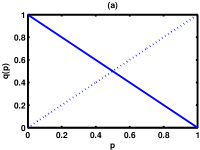
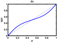
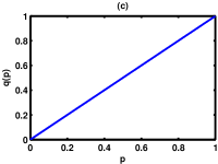
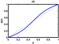
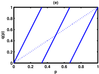
Figure 1: In the reality game, the probability $q$ of the outcome heads is a function of the total fraction of wealth $p$ bet on heads. Figure (a) shows a purely self-defeating map in which the probability of the outcome heads is negatively correlated with the amount bet on heads. The only fixed point of this map, corresponding to a possible equilibrium point for the game, is at $p=1/2$. Figures (b), (c), (d), show positively reinforcing maps where the probability of heads is positively correlated with the amount bet on heads: here, $\alpha$ is a parameter that determines the degree of correlation of the outcome probabilities with the inputs. In (b) $\alpha=1/2$; (c) is the identity map; and in (d) $\alpha=1.5$. Finally, figure (e) shows a multi-modal reality map, $q(p)=3p\mod 1$, with three fixed points.

The parameter $\alpha$ is the slope at $p=1/2$. When $\alpha=0$, $q(p)$ is constant (purely objective), and when $\alpha>0$, $q(p)$ is self-reinforcing. The derivative $q^{\prime}_{\alpha}(1/2)$ is an increasing function of $\alpha$; when $\alpha=1$, $q^{\prime}(1/2)=1$, and $q(p)$ is close to the identity map. We study the self-defeating case separately using the map $q(p)=1-p$. Finally, to study a more complicated example, we study the multi-modal reality map, $q(p)=3p\mod 1$, which has three fixed points.

3 Dynamics of the objective bias

In this section we study the dynamics of the objective bias of the coin, which is the tangible reflection of “reality” in the game. This also allows us to get an overview of the behavior for different reality maps $q(p)$. We use $N=29$ agents each playing one of the 29 equally spaced strategies on $(0,1)$: $1/30,2/30,\dots,29/30$, and begin by giving them all equal wealth. We then play the game repeatedly and plot the bias of the coin $q^{(t)}$ as a function of time. This is done several times using different random number seeds to get a feeling for the variability vs. consistency of the behavior of different reality maps, as shown in Figure 2.

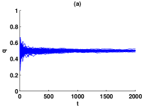
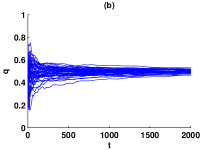
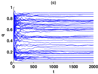
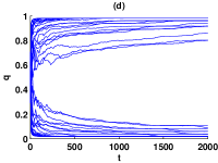
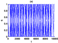
Figure 2: This figure shows how the objective bias $q$ of the coin varies with time $t$ for the different reality maps illustrated in Figure 1. All the players have the same initial wealth. The first player has fixed strategy $p(\text{heads})=1/30$, $p(\text{tails})=29/30$, the second player has fixed strategy $p(\text{heads})=2/30$, $p(\text{tails})=28/30$, etc. Figures (a)–(e) plot the objective bias $q$ of the coin as a function of time using different random number seeds to generate the sequence of coin tosses. Figure (a) shows the self-defeating case, $q(p)=1-p$, corresponding to the reality map of Figure 1(a): here, the objective bias converges rapidly to the fixed point of the map, $p=q=1/2$. Players with this strategy eventually acquire all the wealth. Figure (b) shows the weakly self-reinforcing case $\alpha=0.5$, corresponding to the reality map of Figure 1(b): in this case, the objective bias also converges to the fixed point $p=q=1/2$, albeit more slowly than in the self-defeating case of (a). Figure (c) shows the ‘purely subjective’ case of Figure 1(c), $q(p)=p$: here, all points are fixed points. In the purely subjective case, the map eventually converges to one player’s strategy — the strategy to which it converges is determined randomly from the initial tosses of the coin. Figure (d) shows the strongly self-reinforcing case $\alpha=1.5$ of Figure 1(d): here the objective bias gradually moves either towards the fixed point $q=0$ or to the fixed point $q=1$. Finally, figure (e) shows the behavior under the multi-modal reality map $q(p)=3p~{}\mod~{}1$ shown in Figure 1(e). The bias $q$ oscillates wildly and stochastically back and forth between $0$ and $1$. Although it is not obvious from the figure, over time, the wealth becomes concentrated on strategies $s=1/3$, $s=2/3$.

For the purely objective case $q(p)=1/2$, the result is trivial since $q$ doesn’t change. For the self-defeating case, $q(p)=1-p$, the results become more interesting, as shown in (a). Initially the bias of the coin varies considerably, with a range that is generally about $0.3$ – $0.7$, but it eventually settles into a fixed point at $q=1/2$. For this case the bias tends to oscillate back and forth as it approaches its equilibrium value. Suppose, for example, that the first coin toss yields heads; after this toss, players who bet more on heads possess a majority of the wealth. At the second toss, because of the self-defeating nature of the map, the coin is biased towards tails. As a result, wealth tends to shift back and forth between heads and tails players before finally accruing to players who play the ‘sensible’ unbiased strategy.

We then move to the weakly self-reinforcing case using equation ((5)) with $\alpha=1/2$, as shown in (b). The behavior is similar to the previous case, except that the fluctuations of $q^{(t)}$ are now larger. At the end of $2000$ rounds of the game, the bias is much less converged on $q=1/2$. The bias is also strongly autocorrelated in time — if the bias is high at a given time, it tends to remain high at subsequent times. (This was already true for the self-defeating case, but is more pronounced here.) Although this is not obvious from this figure, after a sufficiently long period of time all trajectories eventually converge to $q=1/2$.

Next we study the purely subjective case, $q(p)=p$, as shown in (c). In this case the bias fluctuates wildly in the early rounds of the game, but it eventually converges to one of the strategies $s_{i}$, corresponding to the player who eventually ends up with all the wealth.

As we increase $\alpha>1$, as shown in (d), the instability becomes even more pronounced. The bias initially fluctuates near $q=1/2$, but it rapidly diverges to fixed points either at $q=0$ or $q=1$. Which of the two fixed points is chosen depends on the random values that emerge in the first few flips of the coin; initially the coin is roughly fair, but as soon as a bias begins to develop, it is rapidly reinforced and it locks in. The extreme case occurs when $q(p)$ is a step function, $q(p)=0$ for $0\leqslant p<1/2$, $q(1/2)=1/2$ and $q(p)=1$ for $1/2<p\leqslant 1$. In this case the first coin flip determines the future dynamics entirely: if the first coin flip is heads, then players who favor heads gain wealth relative to those who favor tails, and the coin forever after yields heads, until all the wealth is concentrated with the player that bets most heavily on heads. (And vice versa for tails.)

Finally, in (e) we show an example of the bias dynamics for the multi-modal map $q(p)=3p\mod 1$. In this case the bias oscillates between $q=0$ and $q=1$, with a variable period that is the order of a few hundred iterations. We explain this behavior at the end of the next section.

4 Wealth dynamics

How do the wealths of individual players evolve as a function of time? The purely objective case $q=\textit{const}$ with fixed strategies and using a bookmaker instead of pari-mutuel betting was studied by Kelly (1956), Cover and Thomas (1991), and Blume and Easley (1993). Assuming all the strategies are distinct, they show that the agent with the strategy closest to $q$ asymptotically accumulates all the wealth. Here “closeness” is defined in terms of the Kullback-Leibler distance between the strategy vector $s_{il}$ and the true probability vector of objective outcomes $q_{l}$.

For all reality maps $q(p)$ that we have studied we find that one player asymptotically accumulates nearly all the wealth. As a particular player becomes more wealthy, it becomes less and less likely that another player will ever overtake this player. This concentration of wealth in the hands of a single player is the fundamental fact driving the convergence of the objective bias dynamics to a fixed point, as observed in the previous section. The reason is simple: once one player has all the wealth, this player completely determines the odds, and since her strategy is fixed, she always places the same bets.

4.1 Purely subjective case

It is possible to compute the distribution of wealth after $t$ steps in closed form for the purely subjective case, $q(p)=p$. The probability that heads occurs $m$ times in $t$ steps is a sum of binomial distributions, weighted by the initial wealths $w_{i}^{(0)}$ of the players,

$$P_{m}^{(t)}=\sum_{j=1}^{N}w_{j}^{(0)}\left[{\binom{t}{m}}s_{j}^{m}(1-s_{j})^{t-m}\right]\,,$$ (6)

and the corresponding wealth of player $i$ is

$$w_{i}^{(t)}=\displaystyle\frac{s_{i}^{m}(1-s_{i})^{t-m}w_{i}^{(0)}}{\sum_{j}s_{j}^{m}(1-s_{j})^{t-m}w_{j}^{(0)}}\,.$$ (7)

When the initial wealths are evenly distributed among the players, no player has an advantage over any other. However, as soon as the first coin toss happens, the distribution of wealth becomes uneven. Wealthier players have an advantage because they have a bigger influence on the odds, so the coin tends to acquire a bias corresponding to the strategies of the dominant (i.e. initially lucky) players. Figure 3 shows the probability $P_{m}^{(t)}$ as a function of $m$ for $t=10^{3}$ and $t=10^{5}$, with $N=29$.

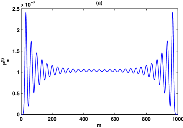
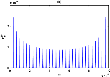
Figure 3: In the purely subjective case, $q(p)=p$, all fixed betting strategies (e.g., betting $1/3$ on heads and $2/3$ on tails) have an equal chance of eventually dominating the game. As before, there are $N=29$ players with the same initial wealth, each playing a different fixed strategy. This figure shows the probability $P_{m}^{(t)}$ as a function of $m$, where $P_{m}^{(t)}$ is the probability that heads occurs $m$ times in $t$ rounds of the game with $q(p)=p$ for (a) $t=10^{3}$ and (b) $t=10^{5}$. After $10^{3}$ tosses in (a), the probabilities of heads occurring $m$ times in $t$ rounds have begun to show pronounced peaks around points $m=t\frac{k}{N+1}$, $k=1,...,29$, which correspond to individual players’ strategies. In (b), after $10^{5}$ tosses, the probabilities of ending close to one of the players’ strategies are very pronounced and clearly separated; also note that, although some peaks are higher than others, the total weight (the integral) of each peak is the same. This means that each fixed betting strategy has the same probability of eventually dominating the game.

After $10^{3}$ steps the binomial distributions are still strongly overlapping, and there is still a reasonable chance to overtake the winning strategy. After $10^{5}$ steps, however, the bias of the coin has locked onto an existing strategy $s_{i}$, due to the fact that this strategy has almost all the wealth. Once this happens, the probability that this will ever change is extremely low.

4.2 Multi-modal reality map

We now explain the peculiar bias dynamics observed in Figure 2(e) for the multi-modal map $q(p)=3p\mod 1$ of Figure 1(e), in which the bias of the coin oscillates wildly between $0$ and $1$. Through the passage of time the wealth becomes concentrated on strategies near either $s=1/3$ or $s=2/3$, corresponding to the discontinuities of $q(p)$. Suppose, for example, that $p=\sum_{i}w_{i}s_{i}$ is slightly greater than $1/3$, where the $q(p)$ map is close to zero. This causes a transfer of wealth toward strategies with smaller values of $s$ until $p=\sum_{i}w_{i}s_{i}<1/3$. At this point the bias of the coin flips because $q(p)$ is now close to one and the transfer of wealth reverses to favor strategies with higher values of $s$. Due to fluctuations in the outcomes of the coin tosses this oscillation is not completely regular. It continues indefinitely, even though with the passage of time wealth becomes concentrated more and more tightly around $s=1/3$. A similar process occurs if the first coin tosses cause convergence around $s=2/3$. We discuss the initial convergence around $s=1/3$ or $s=2/3$ in more detail in Section 6.

5 Analytic analysis of approach to equilibrium

So far, our discussion of the ‘reality game’ has been heuristic and based on simulations. In this section we develop an analytic description of the game when players play fixed strategies. In this simple case the behavior of the game in general, and the approach to equilibrium in particular, admit a closed-form analytic solution.

This section establishes the following features of the reality game with fixed strategies:

• Stable equilibria of the game correspond to fixed points $\tilde{q}=q(\tilde{p})=\tilde{p}$ of the reality map, with $\mu=q^{\prime}(\tilde{p})<1$.

• A central-limit theorem argument shows that the distribution of wealth among the different strategies approaches a Gaussian distribution after many plays of the game.

• The approach to the fixed point is governed by a power law.

The method that will be used is as follows. First, we establish that the wealth distribution tends to a Gaussian. Next, we derive a hierarchy of equations for the approach of the moments of this distribution to the fixed points; in this hierarchy, the rate of approach of the $k$-th moment will depend on the value of the $(k+1)$-th moment. The Gaussian character of the wealth distribution allows us to truncate the hiearchy of equations to obtain coupled ordinary differential equations for the mean and variance. Finally, we solve these equations to show that the approach to equilibrium is governed by a power law. In the process of solution we find that fixed points $\tilde{p}=0,1$ behave differently from fixed points $\tilde{p}\neq 0,1$.

5.1 Wealth updating

Assume a continuum of strategies $\{s\}$, $0\leqslant s\leqslant 1$. Let $w(s)$ be the distribution of wealth over the strategies with $\int w(s)ds=1$. The total amount bet on heads is $p=\int sw(s)ds$. The updating rule is as follows. Let $w_{t}(s)$ be the wealth distribution at time $t$. If the coin comes down heads, from equation ((4)) the new distribution is

$$w_{t+1,h}(s)=sw_{t}(s)/p_{t}.$$ (8)

Similarly, if it comes down tails, the new distribution is

$$w_{t+1,t}(s)=(1-s)w_{t}(s)/(1-p_{t}).$$ (9)

5.2 Wealth distribution approaches a Gaussian

It is simple to show that the wealth distribution $w_{t}(s)$ approaches a Gaussian after many trials. After many trials the distribution is proportional to $s^{m}(1-s)^{n}w_{0}(s)$, where $m$ is the number of heads and $n$ is the number of tails. In the limit as $m$ and $n$ become large, this is an ever narrower binomial distribution multiplied by $w_{0}(s)$: as long as the derivatives of $w_{0}(s)$ are finite, the only part of $w_{0}(s)$ that is important is its value at the peak. Thus the overall distribution tends to a binomial distribution, which asymptotically becomes a Gaussian distribution scaled by the value of $w_{0}(s)$ at the peak. For $m<<n$, we can also use the Poissonian approximation to the binomial distribution. For the analysis below, however, both Poissonian and Gaussian approximations give the same dynamics: accordingly, we will use the Gaussian approximation below.

Suppose that there have been $t$ trials, so that $m+n=t$. The average value of the approximately Gaussian distribution $w_{t}(s)\propto s^{m}(1-s)^{n}w_{0}(s)$ is then $p=m/t$, and the variance of the Gaussian is $D=p(1-p)/t$. This formula for the variance will prove useful for determining the behavior of the game as it approaches equilibrium.

5.3 Dynamics of average bet

Now derive a formula for the change in the amount bet on heads over time. At time $t$, the amount bet on heads is the mean of the wealth distribution, $p_{t}=\int sw_{t}(s)ds$. Define the variance of the distribution to be $D_{t}=\int s^{2}w_{t}(s)ds-p_{t}^{2}$. If the coin comes down heads, then using equation (8) the new value of $p$ is

$$p_{t+1,h}=\int sw_{t+1,h}(s)ds=\int\frac{s^{2}w_{t}(s)}{p_{t}}ds=p_{t}+\frac{D_{t}}{p_{t}}.$$ (10)

That is, if the coin comes down heads, the value of $p_{t}$ is displaced by $D_{t}/p_{t}$ in the heads direction. Equation (10) does not rely on the Gaussian approximation. Inserting the formula $D=p(1-p)/t$, we obtain a formula for the displacement of $p$ in the Gaussian approximation:

$$p_{t+1,h}\stackrel{{\scriptstyle\text{G}}}{{=}}p_{t}+\frac{(1-p_{t})}{t},$$ (11)

where $\stackrel{{\scriptstyle\text{G}}}{{=}}$ indicates equality in the Gaussian approximation.

In the same way, we obtain formulae for the behavior of the system if the coin comes down tails. If the coin comes down tails, the new value of $p$ is

$$p_{t+1,t}=\int\frac{s(1-s)w_{t}(s)}{1-p_{t}}ds=p_{t}-\frac{D_{t}}{1-p_{t}}.$$ (12)

That is, if the coin comes down tails, the value of $p$ is displaced by $D_{t}/(1-p_{t})$ in the tails direction. In the Gaussian approximation, this becomes

$$p_{t+1,t}\stackrel{{\scriptstyle\text{G}}}{{=}}p_{t}-\frac{p_{t}}{t}.$$ (13)

On the $(t+1)$-th toss, the coin comes up heads with probability $q_{t}$ and tails with probability $1-q_{t}$. Define $\Delta p_{t}=p_{t+1}-p_{t}$. Letting $E$ represent the expectation over heads and tails, from equations ((10)) and ((12)) the average change in $p$ is then

$$\operatorname{E}[\Delta p_{t}]=q_{t}p_{t+1,h}+(1-q_{t})p_{t+1,t}-p_{t}=q_{t}\frac{D_{t}}{p_{t}}-(1-q_{t})\frac{D_{t}}{1-p_{t}}=(q_{t}-p_{t})\frac{D_{t}}{p_{t}(1-p_{t})},$$ (14)

and for Gaussian approximation, the corresponding expression is obtained from equations ((11)) and ((13)):

$$\operatorname{E}[\Delta p_{t}]\stackrel{{\scriptstyle\text{G}}}{{=}}q_{t}\frac{(1-p_{t})}{t}-(1-q_{t})\frac{p_{t}}{t}=\frac{q_{t}-p_{t}}{t}.$$ (15)

In the regime where the Gaussian approximation is valid, the system takes a random walk with a step size that decreases as $1/t$.

5.4 Approach to equilibrium

Now employ the functional dependence of $q$ on $p$. In the vicinity of the fixed point $\tilde{q}=q(\tilde{p})=\tilde{p}$, we can use a linear approximation of $q(p)$ and write

$$q_{t}\approx\tilde{q}+\mu(p_{t}-\tilde{q}),$$ (16)

where $\mu=q^{\prime}(\tilde{p})$ is the slope at the fixed point. Substituting the linear approximation of equation ((16)) into the expression for the average change in $p$, equations ((14)) and ((15)), we obtain (after some algebra)

$$\operatorname{E}[\Delta p_{t}]=\frac{D_{t}(\mu-1)(p_{t}-\tilde{q})}{p_{t}(1-p_{t})}\stackrel{{\scriptstyle\text{G}}}{{=}}(\mu-1)\frac{p_{t}-\tilde{q}}{t}.$$ (17)

Defining the distance to the fixed point to be $y=p-\tilde{q}$, and letting $\Delta y_{t}=y_{t+1}-y_{t}$, we now have an equation for the average change in this quantity:

$$\operatorname{E}[\Delta y]=\frac{D(\mu-1)}{p(1-p)}y=\frac{D(\mu-1)}{(\tilde{q}+y)(1-\tilde{q}-y)}y\stackrel{{\scriptstyle\text{G}}}{{=}}(\mu-1)\frac{y}{t}.$$ (18)

From equation ((18)), we see right away that the condition for converging to a fixed point is that the slope at the fixed point, $\mu=q^{\prime}(\tilde{p})$, is less than one. This was also seen numerically in Section 3.

In the Gaussian limit, equation ((18)) shows that the expected change in $y$ from one step to another is linear in $y$. As a result, it can be shown by explicit calculation that the change in $\operatorname{E}[\Delta y_{t}]$ from time $t$ to $t+1$ is equal to $\Delta\operatorname{E}[y_{t}]$, where $\operatorname{E}[y_{t}]$ is the expected value of the distance from the equilibrium point after $t$ time steps. In other words, rather than tracking the entire stochastic process and taking its average value at a time, we can simply construct a differential equation for the average value $\operatorname{E}[y_{t}]$. In particular, averaging again in equation ((18)) then yields an equation for $\operatorname{E}[y_{t}]$:

$$\Delta\operatorname{E}[y_{t}]=(\mu-1)\frac{\operatorname{E}[y_{t}]}{t}.$$ (19)

In the following, for the sake of compactness, define $\bar{y}_{t}=\operatorname{E}[y_{t}]$. Writing equation ((19)) in continuous time gives a differential equation for $\bar{y}$:

$$\frac{d\bar{y}}{dt}=(\mu-1)\frac{\bar{y}}{t}.$$ (20)

In other words, in the Gaussian regime, the approach to equilibrium obeys a power law on average:

$$\bar{y}\propto t^{\mu-1}.$$ (21)

The rate of approach to equilibrium depends on the slope $\mu$ of the reality map $q(p)$ at the fixed point.

5.5 Fluctuations about mean

It is important to keep in mind that equation ((21)) is an equation for the average value of $y$: for any given set of coin flips, there will be fluctuations about that average. These fluctuations are governed by the variance $\Delta_{t}$ of the stochastic process. As noted above, $y$ takes a biased random walk with step size that goes as $O(1/t)$ for late times. These late time fluctuations can be shown to have an average magnitude $\sqrt{p(1-p)/t}$, the same as the fluctuations in the wealth distribution at time $t$.

This estimate of the late time fluctuations does not include the propagation forward in time of earlier fluctuations. Early on in the random walk, the step sizes are larger: later on, they are smaller. The early fluctuations propagate forward in time like $t^{(\mu-1)}$. As we’ll now show, when one adds in all fluctuations that occur at all points in time, these propagating earlier fluctuations combine to give an average fluctuation size of $\Delta_{t}=t^{(\mu-1)/2}$. More precisely, we have the following accounting, using the Gaussian approximation, and the biased random walk of section (5.3).

A fluctuation of size $f$ at time $t_{1}$ propagates over time as $f\times(t/t_{1})^{(\mu-1)}$. Let’s use this feature to propagate forward in time the effect of all fluctuations. At each time step, the magnitude of the fluctuation is on the order of the step size. The first step is of size $O(1)$, the second step is of size $O(1/2)$, the third step is of size $O(1/3)$, etc., with the $k$’th step being of size $O(1/k)$. So our overall fluctuations are of the following order:

$$\Delta_{t}=\pm 1\times\big{(}{t\over 1}\big{)}^{\mu-1}\pm{1\over 2}\times\big{(}{t\over 2}\big{)}^{\mu-1}\pm{1\over 3}\times\big{(}{t\over 3}\big{)}^{\mu-1}\pm\ldots\pm{1\over t}\times\big{(}{t\over t}\big{)}^{\mu-1}=t^{\mu-1}\bigg{(}\pm{1\over 1^{\mu}}\pm{1\over 2^{\mu}}\pm{1\over 3^{\mu}}\pm\ldots\pm{1\over t^{\mu}}\bigg{)}$$ (22)

That is, the $k$’th term in this sum goes as $t^{\mu-1}$ times plus or minus $1/k^{\mu}$. But the typical magnitude of the sum of plus or minus $1/k^{\mu}$ from $1$ to $t$ is on the order of $t^{(1-\mu)/2}$. (This estimated magnitude relies on a Gaussian approximation: the accuracy of this estimate will decline as $\mu\rightarrow 1$ for $\tilde{q}\neq 0,1$, and as $\mu\rightarrow 0$ for $\tilde{q}=0,1$. For future work, it would be useful to obtain analytic solutions for the scaling of the fluctuations in these two limits.) As a result, the estimated magnitude of the early time fluctuations, propagated forward and summed, goes as $\Delta_{t}=O(t^{(\mu-1)/2})$. If $\mu\geqslant 0$, the total fluctuations are dominated by early time fluctuations, propagated forward in time. If $\mu<0$, then it is only the late-time fluctuations that are important, and these go as $t^{-1/2}$, as mentioned above. Since the average distance from a fixed point shrinks as $y_{t}\propto t^{\mu-1}$, and as fluctuations go either as $\Delta_{t}\propto t^{(\mu-1)/2}$ ($\mu\geqslant 0$), or $\Delta_{t}\propto t^{-1/2}$ ($\mu<0$), the actual distance from a fixed point at any time is dominated by fluctuations about the mean value of $y_{t}$.

5.6 Summary

To summarize this section, the reality game with fixed strategies exhibits non-trivial but still analytically tractable behavior. Equilibria correspond to fixed points of the reality map with slope less than one, and the mean distance from those equilibria shrink as a power law in time with exponent $\mu-1$, where $\mu$ is the slope of the reality map at the fixed point. The actual distance from equilibrium at any time is dominated by fluctuations about that mean value.

When players possess non-fixed strategies, the behavior of the game becomes more complicated. Equilibria still exist, however. In the next section, we introduce rational players who change their strategies over time.

6 Rational players and the long-term equilibria

In this section we will show that by introducing an appropriate notion of rational players it is possible to predict the set of possible asymptotically dominant strategies, i.e. the long-term equilibria. To do this we imagine a player who is rational in the strong sense that she not only understands the structure of the game, but also knows all the strategies and wealths of all the other players. The rational player is able to use this information to optimize her play. The players placing bets with fixed strategies are obviously sub-rational in any sense of the word. Such models with a mixture of rational and sub-rational players are often called noise trader models in the finance literature (Shleifer (2000)).

Use of a rational player requires the choice of a utility function. As originally shown by Kelly (1956), logarithmic utility is the unique choice that optimizes the asymptotic growth rate of wealth. If one player’s asymptotic growth rate is higher than that of all the others, that player will end up with all the money. This dictates that for our purpose, which is to predict the asymptotically dominant strategies, we want to consider rational players who maximize log-returns. The choice of other utility functions can be disastrous. For example, maximizing simple returns often dictates betting everything on a single outcome. Doing this an infinite number of times guarantees that eventually some other outcome will be selected and the player will lose all her wealth, which is obviously a poor strategy if one’s goal is to maximize the probability of long-term survival.

6.1 Derivation of optimal strategy

For the case $q=\textit{const}$, as shown in Cover and Thomas (1991), the asymptotic log-returns can be maximized by simply repeatedly maximizing the expected log-return on the next step.

$$\operatorname{E}r_{i}^{(t+1)} = \operatorname{E}\log\frac{w_{i}^{(t+1)}}{w_{i}^{(t)}}$$

$$= \operatorname{E}\log\frac{\pi_{i}}{w_{i}^{(t)}}=\sum_{l}q_{l}\log\frac{s_{il}}{p_{l}}.$$

The reason this works is because when $q=\textit{const}$, the actions of the players do not affect the odds of the coin, and the player does not have to take the future bias of the coin into account in optimizing her strategy. For a more general reality map $q(p)$ that incorporates subjective feedback, this is no longer the case. It is easy to produce examples in which maximizing the log-return two steps ahead produces different results than successively maximizing the log-return a single step ahead. Nonetheless, we find that one step maximization correctly predicts the long-term equilibria. We return to discuss this further later in this section.

Under the assumption of one step maximization, we define a (myopic) optimal player as one that maximizes the expected log-return on the next step. The expected log-return for one step can be written

$$r(s)=q\log\frac{s}{p}+(1-q)\log\frac{(1-s)}{(1-p)},$$ (23)

where as before $q=q_{1}$, and $p=p_{1}$, i.e. these are the values for heads, and $s$ is the bet of the rational player on heads. Recalling that for a discrete strategy set $p=\sum_{i}s_{i}w_{i}$, or for a continuous set $p=\int sw(s)ds$, the first derivative $dr/ds$ is

$$\frac{dr}{ds}=q^{\prime}w\bigg{[}\log s-\log p-\log(1-s)+\log(1-p)\bigg{]}\\ +q\left(\frac{1}{s}-\frac{w}{p}\right)+(1-q)\left(-\frac{1}{1-s}+\frac{w}{1-p}\right),$$ (24)

where $q^{\prime}=dq/dp$.

6.2 Increasing returns

In general the optimal strategy depends on the reality map $q(p)$ and also depends on the wealth of the other players. The optimal strategy can be dynamic, shifting with each coin toss as the wealth of the players changes. This is illustrated in Figure 4. Here we show the expected log-return for a rational player with wealth $w$ playing against a second player with wealth $1-w$, where the second player uses a fixed strategy with $s_{2}=1/2$. We compute the strategy of the rational player by numerically solving $dr/ds=0$, where $dr/ds$ is from equation ((24)).

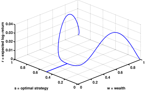
Figure 4: When the game is self-reinforcing the rational strategy is sometimes able to generate increasing returns, i.e. its returns may increase as it gains in wealth. This figure shows the expected log-return $r(s)$ for a rational player with wealth $w$ using a myopic optimal strategy $s$ against a second player with wealth $1-w$ using fixed strategy $s=1/2$. The reality map is strongly self-reinforcing: $q(p)=q_{\alpha}(p)$ for $\alpha=2$. If the optimal player’s wealth is less than $1/3$ her best bet is the equilibrium strategy at $s=1/2$, which only allows her to break even with the fixed strategy player, i.e. her log returns are zero. When her wealth is more than this, however, the fixed point becomes unstable and she can use her ability to influence the objective probability to drive it away from $q=1/2$ and towards one of the two other fixed points $q=0$ or $q=1$, thereby making profits at the expense of the fixed strategy player.

When the rational player’s wealth is low, $s=1/2$ is the optimal strategy, and she can only break even with the fixed player. As the rational player gains in wealth, two strategies on either side of $s=1/2$ become superior, and the rational player makes positive log-returns. As her wealth $w$ increases, the optimal strategies become more and more separated from $s=1/2$, and in the limit as $w\to 1$ the optimal strategy is either $s=0$ or $s=1$.

6.3 Equilibria

The equilibria of the game can be simply computed by noting that that in equation ((24)) a sufficient condition for $dr/ds=0$ is $s=q=p$, i.e. the strategy corresponding to the fixed point $q=p$. This may or may not be stable, depending on the condition of the second derivative. When it is stable, however, it corresponds to an attracting fixed point. This will be stable when the second derivative satisfies

$$\frac{d^{2}r}{ds^{2}}=\frac{1-w}{s(1-s)}\bigg{[}2wq^{\prime}-(1+w)\bigg{]}<0.$$ (25)

When all the wealth is sufficiently closely concentrated around the equilibrium a rational player need only play the equilibrium strategy. This can easily be seen by assuming that the rational player begins with a very small amount of wealth. The approach to equilibrium is then dominated by the fixed-strategy players, and the rational player simply plays the optimal strategy $s^{(t)}=q^{(t)}$. She does not begin to dominate the overall wealth until the game has come close to the fixed-strategy equilibrium.

What happens once the rational player obtains most of the wealth? If this player started off with only a small amount of wealth, then she does not dominate until the game has approached very closely to a particular fixed-strategy equilibrium. But at this point the wealth of the fixed strategy players is concentrated around the equilibrium strategy, and thus is close to the strategy of the rational player. Consequently, once the game is close to a fixed-strategy equilibrium, the fact that the rational player has acquired most of the wealth makes little difference to the approach to equilibrium.

More precisely, let $y=p-\tilde{q}$ be the distance from the equilibrium point, as before. The optimum strategy $p=q(\tilde{p}+y)$ adopted by the rational player is by definition a local maximum of the expected log-return $r$, as discussed above. The expected log-return of a player at the actual equilibrium point, compared with that of the rational player, is then $r+(d^{2}r/ds^{2})y^{2}$, where $d^{2}r/ds^{2}$ is defined in equation ((25)) above. That is, the deviation of the log-return of the fixed-strategy player at the equilibrium point from the log-return of the rational player goes as second order in $y$, and can be neglected in the regime where the analysis of the previous section on fixed strategies holds true. Accordingly, even in cases where the rational player acquires most of the wealth, as long as this does not happen until the game is already close to a fixed point, we expect the power-law approach to equilibrium to hold to a high degree of accuracy.

Note also that the multimodal map $q(p)=3p\mod 1$ is interesting because all the intersections with the identity are local minima for the expected log-return. Instead, the system is attracted to the discontinuities of the map at $s=1/3$ and $s=2/3$. It is as if one can think of the discontinuities of the map as being connected (with infinite slope), creating intersections with the identity that yield local maxima of the log-return.

6.4 Single step vs. multi-step optimization

Under some circumstances it is possible to decompose the optimization into a series of single step optimizations. To see this, consider in more detail the decomposition of the $T$-step log-return into a series of one step returns. Let $r_{t}=r(s_{i}^{(t)},p_{t})$ be the expected log-return for strategy $s_{i}$ on step $t$. This depends on the strategy $s_{i}^{(t)}$ used by player $i$ and the amount $p_{t}$ wagered on heads by all the players on step $t$. Let $S_{i}^{(t-1)}=(s_{i}^{(1)},s_{i}^{(2)},\ldots,s_{i}^{(t-1)})$ be the sequence of strategies used by player $i$ on all previous steps. For a non-constant reality map $q(p)$ the returns depend on the wagers of the players, which in turn depend on their wealths, which depend among other things on the previous moves of player $i$. To emphasize this we write $p_{t}=p(w_{t}(S^{(t-1)}))$. We can write the log-return over $T$ steps as

$$R_{T}=\sum_{t=1}^{T}r(s^{(t)},p(w_{t}(S^{(t-1)}))).$$ (26)

This makes it clear why in general finding a strategy that maximizes log-returns over $T$ steps is challenging: to properly optimize it is necessary to take into account how the bet at $t=1$ influences the wealth of all other strategies at all future times. In some cases, however, this difficult optimization problem can be finessed. Consider the case where player $i$ has negligibly small wealth at time $t=1$. Because $i$’s wealth is negligible, it has no influence on the wealth of the other strategies, and $p_{t}$ is independent of $S^{(t-1)}$ for this player. In this case, player $i$ can optimize over a horizon of length $T$ by performing a series of successive single step optimizations, even when $q(p)$ is not constant. At the beginning of the game, when there are many players, each of whose wealths is small, and to a reasonable approximation all players can optimize their strategies over a horizon of length $T$ by performing single step optimizations.

7 Efficiency

As the game is played the reallocation of wealth causes the population of players to become more efficient in the sense that there are poorer profit opportunities available for optimal players. This is analogous to financial markets, where standard dogma asserts that wealth reallocation due to profitable vs. unprofitable trading will result in a market that is efficient in the sense that all excess profit-making potential has been removed. One would like to be able to measure market inefficiency, and to study the transition from an inefficient to an efficient market. In this section we introduce a quantitative measure of inefficiency, study how it converges in time, and show that it exhibits interesting scaling properties. In particular, the degree of inefficiency converges as a power law, and converges more slowly when there is a higher level of subjective feedback.

7.1 Definition of inefficiency

We define the inefficiency of our game to be the log-return for a rational $\epsilon$ player. Like the rational player discussed in the previous section, this player knows the strategies of all other players, and pursues an optimal strategy that maximizes her expected log-returns. In addition, this player has infinitesimal wealth $\epsilon$, so that her actions have a negligible effect on the outcome of the game. As described in the previous section, the assumption of infinitesimal wealth is convenient because it means that the player need only optimize one step ahead, and because it guarantees that the rational $\epsilon$ player does not affect the wealth dynamics of the game. The log-return for the rational $\epsilon$ player defines the inefficiency at every time step.

In the purely objective setting where $q=\textit{const}$, the approach to efficiency is guaranteed by the fact that the wealth dynamics are formally equivalent to Bayesian updating, implying all the wealth converges on the correct hypothesis about the bias of the coin. For more general settings this is no longer obvious, as there is no longer such a thing as an objectively correct hypothesis. Nonetheless, we always find the system converges to an equilibrium where all the wealth is concentrated on a single point. At equilibrium there are no profit opportunities for the rational $\epsilon$ player, and thus the market is perfectly efficient.

7.2 Numerical study of inefficiency vs. time

We have studied the approach to efficiency numerically for a variety of different reality maps, as shown in Figure 5.

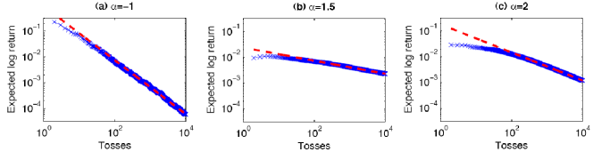
Figure 5: The expected log-return to a rational $\epsilon$ player is plotted as a function of time, measured as the number of tosses of the coin. This provides a measure of the inefficiency of the wealth allocation in the game, which diminishes as the system converges to equilibrium. A rational $\epsilon$ player is one who follows an optimal strategy but whose total wealth is too small to affect the outcome. As the game continues the return to an optimal player goes down because the wealth is reallocated to players with better strategies. In these simulations there are $N=3000$ fixed strategy players whose wealth is initially evenly distributed. After an initial transient period the expected log return decreases as a power law in the number of tosses. Since the exponent is less than one, convergence is extremely slow. This depends on the degree of subjectivity of the map: the more subjective (i.e., the closer the map is to $q(p)=p$), the slower the convergence to efficiency. In (a), function $q(p)=1-p$ is used; in (b) and (c) $q(p)=q_{\alpha}(p)$ is used, with the values of $\alpha$ specified in the figures.

To damp out the effect of statistical fluctuations from run to run we take an ensemble average by varying the random number seed. For these simulations, in order to get good scaling results across the whole time interval we used $N=3000$, much larger than $N=30$ as used previously. In all but the purely subjective case we find that the efficiency is a decreasing function of time, asymptotically converging as a power law $t^{-\gamma}$ with $0\leqslant\gamma\leqslant 1$. For the purely objective case $q(p)=1/2$, or for the self defeating case $q(p)=1-p$ we observe $\gamma\approx 1$. In other cases we observe $\gamma<1$, with gamma always in the range $0\leqslant\gamma\leqslant 1$. See Table 1 for some examples.

reality map	$\alpha=2$	$\alpha=1.5$	$\alpha=0.75$	$\alpha=0.5$	$q(p)=\mbox{const}$	$q(p)=1-p$
observed $\gamma$	0.42	0.2	0.13	0.49	0.99	1.03
predicted $\gamma$	0.30	0.23	0.25	0.5	1	1

Table 1: Comparison of numerical vs theoretical predictions of the rate of convergence of the inefficiency to equilibrium, which goes as $t^{-\gamma}$. The first row specifies the reality map; the first four columns refer to the parameter $\alpha$ in equation (5). The second row contains the results of numerical simulations, while the third row contains the predictions of the theory.

7.3 Analytic proof of power law convergence to efficiency

Our numerical results suggest that the approach to efficiency is described by a power law. We now prove this analytically by building on the results obtained in Section 5.

The expected log-return of a player with strategy $s$ was given by equation ((23)) above: $r(s)=q\log\frac{s}{p}+(1-q)\log\frac{(1-s)}{(1-p)}.$ Taking the derivative of $r(s)$ for an $\epsilon$ player, we note that, because her wealth is infinitesimal, neither $p$ nor $q$ depend on her strategy, and we have

$$\frac{dr}{ds}=\frac{q}{s}-\frac{1-q}{1-s}.$$ (27)

Accordingly, a rational $\epsilon$ player maximizes her average log return by playing $s=q$.

In the vicinity of a fixed point $\tilde{q}=\tilde{p}$, the fraction bet on heads can be written $p=\tilde{q}+(p-\tilde{q})=\tilde{q}+y$, and the probability of heads can be written $q=\tilde{q}+\mu(p-\tilde{q})=\tilde{q}+\mu y$, where $\mu=q^{\prime}(\tilde{p})$ is the slope of the reality function at the fixed point, as above. Written in terms of $\tilde{q},\mu$ and $y$, the expression for the expected log-return becomes

$$r=(\tilde{q}+\mu y)\log\frac{\tilde{q}+\mu y}{\tilde{q}+y}+(1-\tilde{q}-\mu y)\log\frac{1-\tilde{q}-\mu y}{1-\tilde{q}-y}.$$ (28)

Assuming that we are close to the fixed point (i.e. $y$ being small), we can expand equation ((28)) to second order in $y$ for small $y$. The expansion takes a different form depending on whether $\tilde{q}$ is in the interior of the interval $[0,1]$ or at one of the endpoints. When $\tilde{q}$ lies in the interior, $\tilde{q}\neq 0,1$, equation ((28)) yields

$$r=\frac{1}{2}(1-\mu)^{2}\bigg{(}\frac{1}{\tilde{q}}+\frac{1}{1-\tilde{q}}\bigg{)}y^{2}+O(y^{3})=\frac{1}{2}(1-\mu)^{2}Cy^{2}+O(y^{3}),$$ (29)

where $C=1/\tilde{q}(1-\tilde{q})$.

The behavior of the average log-return depends on the distance from equilibrium in the vicinity of the fixed point. This distance is dominated by fluctuations as described in Section 5 above. Because these fluctuations obey a power law, the average log-return also obeys a power law. The exponent in the power law depends on the slope of the reality map at the fixed point, and on whether the fixed point is in the interior of the interval or whether it is one of the boundary points at $0$ or $1$. For comparison to the numerical results it is useful to note that for the reality map of equation (5) the slope $\mu=q^{\prime}(\tilde{p})=\alpha$ for the fixed point at $p=1/2$ and $\mu=8/(\pi^{2}\alpha)$ for the fixed points at $p=0$ or $p=1$. We also remind the reader that we do not expect our estimates of $\gamma$ to be accurate when the fixed point is in the interior and $\mu\approx 1$ or when it is on the boundary and $\mu\approx 0$.

Depending on the reality map, the log-return of the rational $\epsilon$ player approaches zero as $t^{-\gamma}$ as follows.

• If $\tilde{q}\neq 0,1$, and $\mu<0$ then $\gamma=1$. The average distance from equilibrium in this case goes as $\Delta_{t}\propto t^{-1/2}$. Accordingly the average value of $y^{2}$ in equation ((29)) goes as $\propto t^{-1}$: the average log-return obeys power law with exponent $-1$. This is true, for example, for the objective case $q(p)=\mbox{const}$ and the self-defeating case $q(p)=1-p$. (See Table 1 and Figure 5(a)).

• If $\tilde{q}\neq 0,1$ and $\mu\geqslant 0$ then $\gamma=(1-\mu)$. The average value of $y^{2}$ in this case is dominated by $\Delta_{t}^{2}\propto t^{(\mu-1)}$. This is the case for $\alpha=0.5$ and $\alpha=0.75$ in Table 1. For $\alpha=0.5$ the agreement is quite good, but as expected, for $\alpha=0.75$, where $\mu=0.75$, we are closer to the critical value $\mu=1$ and the agreement is not as good.

• If $\tilde{q}=0$ or $\tilde{q}=1$ then $\gamma=(1-\mu)/2$. In this case the expansion in small $y$ yields

  $$r=(1-\mu+\mu\log\mu)y+O(y^{2}).$$ (30)

  Once again, the typical distance from the fixed point goes as the average fluctuation size, $\Delta_{t}\propto t^{(\mu-1)/2}$, and so does the expected log-return for a rational $\epsilon$ player. SeeTable 1 with $\alpha=1.5$ and $\alpha=2$ and Figure 5(b) and (c). Agreement is good for $\alpha=1.5$, but as expected for $\alpha=2$, where $\mu$ is closer to zero, the agreement is not as good.

To summarize, for self-defeating or purely objective reality maps $\gamma=1$. For self-reinforcing reality maps, as we approach the purely subjective case where $\mu=1$, $\gamma\to 0$. Thus, the converge of the inefficiency to zero is always slow, but when the reality map is strongly subjective, it is extremely slow.

8 Summary

We have introduced a very simple evolutionary game of chance with the nice property that one can explicitly study the influence of the player’s actions on the outcome of the game. By altering the reality map $q(p)$ it is possible to continuously vary the setting from completely objective, i.e. the odds are independent of the players’ actions, to completely subjective, i.e. the odds are completely determined by the players’ actions.

It has long been known that subjective effects can play an important role in games, causing problems such as increasing returns and lock-in to a particular outcome due to chance events. This game illustrates these effects nicely, making it possible to study both positive and negative feedback.

Perhaps the nicest feature of this game is that it provides a setting in which to study the progression from an inefficient to an efficient market. We have introduced a method of measuring the inefficiency of the game when it is out of equilibrium that is similar to how one might quantitatively measure the magnitude of the arbitrage opportunities for an optimal player in a financial market. As time goes on the game tends to become more efficient, with the inefficiency dying out as a power law of the form $t^{-\gamma}$. As shown in the previous section, $\gamma$ is always in the range $0\leqslant\gamma\leqslant 1$. For self-defeating or purely objective reality maps $\gamma=1$. This already implies a very slow convergence to efficiency. When the reality map is close to being subjective, however, $\gamma\to 0$, implying extremely slow convergence.

One might consider several extensions of the problem studied here. For example, one could study learning (see e.g. Sato et al. (2002)). Another interesting possibility is to allow more general reality maps, in which $q$ is a multidimensional function with a multidimensional argument that may depend on the bets of individual players. For example, an interesting case is to allow some players, who might be called pundits, to have more influence on the outcome than others. It would also be very interesting to modify the game so that it is an open system, e.g. relaxing the wealth conservation condition and allowing external inputs. This may prevent the asymptotic convergence of all the wealth to a single player, creating more interesting long-term dynamics.

References

- Akiyama and Kaneko (2000) Akiyama, Eizo and Kaneko, Kunihiko, 2000. Dynamical systems game theory and dynamics of games. Physica D, 147, 221–258.
- Alos-Ferrer and Ania (2005) Alos-Ferrer, C. and Ania, A.B., 2005. The asset market game. Journal of mathematical economics, 41, 67–90.
- Anufriev et al. (2006) Anufriev, M., Bottazzi, G. and Pancotto, F., 2006. Equilibria, stability and asymptotic dominance in a speculative market with heterogeneous traders. Journal of Economic Dynamics and Control, 30, 1787–1835.
- Arthur et al. (1983) Arthur, B., Ermoliev, Y.M. and Kaniovski, Y.M., 1983. The generalized urn problem and its application. Kibernetika, 1, 49–56.
- Arthur (1994a) Arthur, W. Brian, 1994a. Increasing returns and path dependence in the economy. Ann Arbor: University of Michigan Press.
- Arthur (1994b) Arthur, W. Brian, 1994b. Inductive reasoning and bounded rationality. The American Economic Review, 84, 406–411.
- Blume and Easley (1993) Blume, L. and Easley, D., 1993. Economic natural selection. Economics Letters, 42, 281–289.
- Blume and Easley (1992) Blume, Lawrence E. and Easley, David, 1992. Evolution and market behavior. Journal of Economic Theory, 58, 9–40.
- Blume and Easley (2002) Blume, Lawrence E. and Easley, David, 2002. Optimality and natural selection in markets. Journal of Economic Theory, 107, 95–135.
- Breiman (1961) Breiman, L., 1961. Optimal gambling systems for favorable games, in: Neyman, J. (Ed.), Fourth Berkeley Symposium on Math. Statisics and Probability, volume 1. University of California, pp. 65–78.
- Challet and Zhang (1997) Challet, D. and Zhang, Y. C., 1997. Emergence of cooperation and organization in an evolutionary game. Physica A, 246, 407–418.
- Cherkashin (2004) Cherkashin, Dmitriy, 2004. Perception game. Ph.D. Thesis. University of Chicago.
- Cover and Thomas (1991) Cover, Thomas M. and Thomas, Joy A., 1991. Elements of Information Theory. Wiley series in telecommunications. New York: John Wiley & Sons, Inc.
- Dosi and Kaniovski (1994) Dosi, G. and Kaniovski, Y.M., 1994. On “badly behaved” dynamics: Some applications of generalized urn schemes to technological and economic change. Journal of Evolutionary Economics, 4, 93–123.
- Hens and Schenk-Hoppe (2005a) Hens, T. and Schenk-Hoppe, K., 2005a. Evolutionary finance: introduction to the special issue. Journal of mathematical economics, 41, 1–5.
- Hens and Schenk-Hoppe (2005b) Hens, T. and Schenk-Hoppe, K., 2005b. Evolutionary stability of portfolio rules in incomplete markets. Journal of mathematical economics, 41, 43–66.
- Hommes (1991) Hommes, C., 1991. Adaptive learning and roads to chaos: The case of the cobweb. Economics Letters, 36, 127–132.
- Hommes (1994) Hommes, C., 1994. Dynamics of the cobweb model with adaptive expectations and non-linear supply and demand. Journal of Economic Behavior and Organization, 24, 315–335.
- Kelly (1956) Kelly, J. L., 1956. A new interpretation of information rate. The Bell System Technical Journal, 35, 917–926.
- Keynes (1936) Keynes, J.M., 1936. The general theory of employment, interest and money. London: Macmillan.
- Miller (2005) Miller, M., 2005. Strategy-based wealth distributions. Technical Report. Santa Fe Institute.
- Sandroni (2000) Sandroni, A., 2000. Do markets favor agents able to make accurate predictions? Econometrica, 68, 1303–1341.
- Sato et al. (2002) Sato, Yuzuru, Akiyama, Eizo and Farmer, J. Doyne, 2002. Chaos in learning a simple two-person game. Proc. Natl. Acad. Sci. USA, 99, 4748–4751.
- Shleifer (2000) Shleifer, A., 2000. Clarendon Lectures: Inefficient Markets. Oxford: Oxford University Press.
- Soros (1987) Soros, George, 1987. The Alchemy of Finance. John Wiley and Sons.