A quantitative characterisation of functions with low Aviles Giga energy on convex domains
Andrew Lorent
Mathematics Department
University of Cincinnati
2600 Clifton Ave.
Cincinnati
Ohio 45221
lorentaw@uc.edu
Abstract.
Given a connected Lipschitz domain we let be the subset of functions
in with on and whose gradient (in the sense of trace) satisfies where
is the inward pointing unit normal to at .
The functional
minimised over serves as a model in connection with problems in liquid crystals and thin film blisters, it is also
the most natural higher order generalisation of the Modica Mortola functional. In [Ja-Ot-Pe 02] Jabin, Otto, Perthame characterised a class of functions which includes all limits of sequences with
as . A corollary to their work is that if there exists such a sequence for a bounded
domain , then must be a ball and (up to change of sign) . We prove a quantitative generalisation of this corollary for the class of bounded convex sets.
There exists positive constant such that if is a convex set of diameter and
with then for some and
A corollary of this result is that there exists positive constant such that if
is convex with diameter and boundary with curvature bounded by , then for any minimiser of over ,
where . Neither of the constants or are
optimal.
Key words and phrases:
Aviles Giga functional
2000 Mathematics Subject Classification:
49N99
1. Introduction
We consider the following functional
(1)
the study of which arises from a number of sources, one of the earliest and most important
is the article by Aviles, Giga [Av-Gi 87]. We will refer to the quantity as the Aviles-Giga
energy of functional .
Functional is usually minimised over the space of functions where
and on (in the sense of trace) where is the inward pointing
unit normal, we will denote this space of functions by .
Aviles, Giga raised the problem of the study of the limiting behavior of as
in connection with the theory of smectic liquid crystals [Av-Gi 87]. In [Gi-Or 97] Gioia, Ortiz studied
as a model for thin film blisters. Jin, Kohn [Ji-Ko 00] introduced the by now classic method of
estimating the energy by ‘divergence of vectorfields’.
A related functional arising from micromagnetics was studied by Riviere, Serfaty [Ri-Se 01], in this
case the functional acts on vector fields (in two dimensions) satisfying in
and the functional is given by where is vectorfield extended
trivially by outside . For the Aviles Giga functional we minimise
over curl free vector fields and the functional forces the norm of the vector field to be close to with weighting
while constraining an multiple of the norm (squared) of the gradient, on the other hand
the micromagnetics functional is minimised over vectorfields whose norm is taken to be from the outset and
the functional forces the vector field to be divergence free with weighting
111the term is the norm of the Hodge projection
onto curl free vector fields while again
constraining an multiple of the norm (squared) of the gradient. Functional is much more
rigid and very much stronger results are known for it than for , see [Al-Ri-Se 02],[Ri-Se 01],[Am-Ki-Ri 02], [Am-Le-Ri 03].
Roughly speaking, the conjecture is that as the energy of minimisers of
will converge to a collection of curves on which the gradient of the minimisers make a jump of order
perpendicularly across the curve. This has already been proved for functional [Ri-Se 01]. A way to think
about this is the following, given a connected Lipschitz domain let be the distance from
and let be convolved by a convolution kernel of diameter , the regions
where will be exactly the neighborhoods of the curves on which has a
jump discontinuity. If is a ball will have a discontinuity only at one point, in
all other cases there will be non trivial curves of singularities and for the specific function
, it is exactly in an neighborhood of these curves that the energy
will concentrate. The conjecture is that what we can observe directly for will
hold true for the minimisers of .
The most natural way to study
these questions is within the frame work of convergence. One of the earliest successes of
convergence was the characterisation of the limit of the so called Modica Mortola functional
which is minimised
over scalar functions satisfying an integral condition of the form . It was
shown by Modica, Mortola [Mo-Mo 00] (confirming a conjecture of DeGiorgi)
that the limit of is a constant multiple of the measure of the
jump set minimised over the space of functions
. Given the elementary inequality
(2)
we have that for any sequence of equibounded energy (for some
subsequence ) has a uniform control of and the measure we
obtain as the limit of this sequence of gradients will naturally be supported on the jump set of the
limiting function. In some sense the nature of the limit of could be anticipated from
(2).
Functional is the most natural higher order
generalisation of , in the case of the conjectured limit is
surprising, this is part of the reason that functional has received so much attention. The
first works on identifying the limit are by Aviles, Giga [Av-Gi 87] and Jin, Kohn [Ji-Ko 00],
later these
ideas were developed by Ambrosio, DeLellis, Mantegazza [Am-De-Ma 99], roughly speaking the limiting function space
is conjectured to have a structure similar to the space of functions whose gradient is and
the limiting energy is conjectured to have the form .
Much progress has been made on this conjecture, particularly equi-coercivity of has been
shown independently in [Am-De-Ma 99] and in the work of Desimone, Kohn, Muller, Otto [De-Ko-Mu-Ot 00].
A proposed limiting function space and limiting functional
as been suggested in [Am-De-Ma 99] and it was shown
that all limits of sequences of functions with
are such that and . The compactness proofs provided by [De-Ko-Mu-Ot 00] and [Am-De-Ma 99] are different but
share some common ideas. The proof by [De-Ko-Mu-Ot 00] identifies the set
of all smooth functions for which there exists smooth such that
(3)
influenced by ideas of Tartar and Murat on compensated compactness [Ta 79] [Mu 78] the authors are able to
prove that this set of is sufficiently rich so as to force to converge strongly. In
[Av-Gi 87] the authors (building on work of Jin Kohn [Ji-Ko 00]) found two third order
polynomial vector fields and such that
(4)
Using some elementary and surprising identities satisfied by a different approach to
compactness was found. Rather naturally considering (4), the function space proposed
by [Am-De-Ma 99] is given by the set of functions for which forms a Radon measure for
and the limiting energy functional is given by the total absolute value of this measure on .
Given vector field let , Jabin, Perthame [Ja-Pe 97] showed
that gradients of sequences of bounded Aviles-Giga energy (in fact their method extends to more general
functionals) are compact and the limit satisfies a kinetic equation of the form
where is the distribution derivative with respect to of some measure on and is the rotation given by .
By application of kinetic averaging lemmas [Di-Li-Me 91] this
leads to some regularity; for all ,
and using the kinetic equation a different proof of compactness was found.
The kinetic equation deduced by [Ja-Pe 97] was motivated by the characterisation of the set of
satisfying (3) given in [De-Ko-Mu-Ot 00], indeed defining for
and otherwise, in [De-Ko-Mu-Ot 00] it was shown that a sequence satisfying (3) could
be found that approximates pointwise. Using the kinetic equation deduced in [Ja-Pe 97],
Jabin, Otto, Perthame [Ja-Ot-Pe 02] were able to characterise zero energy limits (and the domains that
allow them) for , in fact their result is stronger, they showed that if a divergence free
vector field satisfies the kinetic equation , a.e. in
and on then either is a strip and is a
constant or for some , and or . An analogous result for zero energy limits of is stated in [Le-Ri 02] and is a consequence of
the main theorem of [Am-Le-Ri 03].
As a corollary, given a sequence and such that
as , letting be the limit of this sequence, the vector field satisfies
the hypothesis stated and hence we have (up to a sign) a complete description of .
The main theorem of this paper is a quantitative generalisation of the corollary to Jabin, Otto, Perthame
theorem over the class of bounded convex sets.
Theorem 1.
Let and be a convex domain with diameter . Let
with on and
of (in the sense of trace) where is the inward
pointing unit normal. Then there exists positive constants and such that for some
,
and
Corollary 1.
Let and be a convex set of diameter and with boundary and curvature bounded above by . Let . There exists
positive constants and such that if is a minimiser of over , then
(5)
where .
In Theorem 1 we take and in Corollary 1, . Neither constant is
optimal. Corollary 1 requires a fair amount of technical work establishing an upper bound for the minimizer of in terms
of the ‘eccentricity’ . For the reader primarily interested in the asymptotic behavior
of minimizers as recent powerful results on -convergence upper bound of
(in the case where the function being approximated satisfies ) by Conti, DeLellis [Co-De 07] and Poliakovsky [Po 07] do much
of the work for us and we can give a relatively shorter proof of the following corollary to Theorem 1. Note that Corollary 2 stated
below is a corollary to Corollary 1.
Corollary 2.
Let be a convex set of diameter with boundary. Let be
as defined in Corollary 1. There exists
positive constants and such that if is a minimiser of over , then
(6)
where .
Plan of paper. After the introduction in Section 1 we sketch the proof
of the main theorem in Section 2. In Section 3 we prove the main theorem. In Section 4 we establish Corollary 2, the additional lemmas needed to establish Corollary 1 are given in Section 5.
1.1. Background
Given a sequence and with , let
be the limit of , the vector valued measure given by
(where are the third order
polynomial vector fields that satisfy (4)) gives us the expression of the limiting energy, i.e. . If we consider
the -dimensional part of the measure
it has been shown that is -rectifiable [De-Ot 03] (see also [De-Ot-We 03])
and an analogous result has been shown for [Am-Ki-Ri 02]. It was also
shown has jump discontinuous across the rectifiable set exactly as would be the
case if was and its jump set was given by . However it is not known (even if are the minimisers of ) if measure is even singular with respect to Lebesgue measure. Note that
for the function the minimiser of the limiting energy is known to be rectifiable
[Am-Le-Ri 03], for a sequence with only equibounded energy the measure is not known to be singular.
The original motivation for Theorem 1 was to prove a version of it for without
boundary conditions, under the hypotheses ,
and
,
the conclusion in this case would be that there exists a smooth function with
everywhere such that for some
. This is a kind of quantitative version of the main proposition required to prove compactness in
[Am-De-Ma 99], (see Proposition 4.6). The hope is to use such a quantitative result to show is singular, or at least that is continuous at a.e. point outside , we will address these issues in a forthcoming
paper [Lo pr].
The many strong results about measure (and the measure that gives the limiting functional
for the micromagnetics function) have been achieved by characterising various
kinds of blow up of the measure and understanding well the absolute (i.e. non quantitative)
situation in the limit [Am-Ki-Ri 02], [De-Ot 03], [De-Ot-We 03], [Ja-Ot-Pe 02], [Am-Le-Ri 03]. In some
sense there are only two possibilities, to take a limit and have an absolute situation
and to understand the measure from this, or to stop before the limit and have a non-absolute situation
and try and understand something about it with a quantitative theorem. Our primary motivation
in proving a quantitative version of Jabin-Otto-Perthame Theorem was so as to obtain
a result that could be used for the latter approach.
By Poincare’s inequality it is easy to see and so
Theorem 1 follows from the following slightly more general result.
Theorem 2.
Let be a convex body centered on with . Let , suppose
is a function satisfying
(7)
and
(8)
and in addition satisfies on and on in the sense of trace
where is the inward pointing unit normal to at .
Then there exists positive constant such that
and
(9)
Acknowledgments. Part of this paper was written while the author was
the Emma e Giovanni Sansone Junior Visitor at Centro
di Ricerca Matematica Ennio De Giorgi, Pisa.
The hospitality and support this institute is gratefully acknowledged. I would also like to express my great thanks to the referee for numerous suggestions, simplifications and
improvements. The quality of the paper has been substantially increased by the input of the referee.
While the proof for convex domains is slightly involved, there are only a couple
of ideas that are really central. We will sketch the proof for the case , ignoring
(without comment) many technicalities in order to give an impression of the basic skeleton.
The real engine of the proof is the characterisation in [De-Ko-Mu-Ot 00] of the set of such that (3) is satisfied.
As mentioned in the introduction, as consequence of the characterisation it was shown there exists a sequence
of satisfying (3) that converge pointwise to the function for
and otherwise. Following closely the proof of this
it is possible to extract the existence of functions and with
, ,
such that the following two inequalities hold.
Let for and otherwise,
(10)
and (letting be the anti-clockwise rotation)
(11)
Recall, for simplicity we have taken , as on then
we can extend to a function such that
and
(12)
It is more convenient to work with vectorfields that are almost curl free instead of
almost divergence free. So notice that (10) can be rewritten as
(13)
and we have
.
By the quantitative Hodge decomposition type theorem from [Am-De-Ma 99] (Theorem 4.3) we can find a scalar valued
function such that
(14)
The real power of (14) is that on the annulus we
know that and hence given inequality (13) (and the fact that
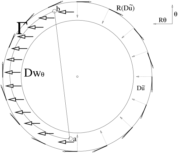
on ) we have a that for any , see figure 1.
Figure 1.
In much the same way in the ball , by inequalities (13), (14) and we have that there exists a large set , with such that if then
or
depending on whether or .
It is not hard to see we can find points with
, , the angle between and is at least
and . Let and . As can be seen
from figure 1 we can connect to with a path so
So by arguing in the same way for lines parallel to by Fubini’s theorem we can show
.
Thus all but points are such that
. As is arbitrary we can rephrase this the following way.
Given for all but points are such that
.
Now take . For all
but points in we have that
and , it is not hard to show this implies and since and we have with an exceptional set of measure less than .
So integrating a carefully chosen line inside
and using the fact that on we can show
.
Now since is mostly very close to and we have zero boundary condition, so avoiding technicalities
assuming the coarea formula we have . Note also that for any , so by the fundamental theorem of
Calculus
so
(17)
This concludes the sketch of the proof of Theorem 2.
2.2. Sketch of the proof of Corollary 1 and Corollary 2
In order to deduce Corollary 1 we need to apply Theorem 1 to the minimizer
of over . We can only do this if the minimizer has small energy (and from
Theorem 1 we know it can only have small energy if is close to a ball). For this reason it is
necessary to construct a function in with this property.
It turns out this is a surprisingly delicate task, it is achieved in
Section 4 and Section 5 of the paper.
The obvious way to attempt the construction is to make some adaption of the function
, this function clearly satisfies the correct boundary condition. The
first problem is that will have its gradient in BV and it is easy to construct examples of convex domains that are
close to balls for which the singular part of is widely spread over the domain. So
it is necessary to convolve , let denote the convolution of
with a convolution kernel of support size .
We need to check that the function we obtain
by convolving will have small energy. By recent results of [Am-De 03] we
have that . So by Poincare inequality if for most balls the gradient of is not too concentrated in balls of sized then
we would have is small. Now
assuming is close to a ball, then for not too close to the center of
(which we assume is ) it is not hard to show that is small. By convexity of , if is a
parameterization of then
will
be a monotonic parameterization of . So the total variation of
can be explicitly bounded above. The closer is to a ball the better the estimate on holds but near the center it breaks down. To overcome this we do the following. Let
and let
, so is roughly a ball centered on of radius .
So defining we have
a.e. and . Notice that . Now is a convex set of diameter approximately
so . So we have the estimate so
for any . Now by convexity of and hence monotonicity
of the gradient along the level set we can prove an explicit
upper bound . So
we can estimate
(18)
Putting these things together we have . This allows us to apply recent results on -upper bounds of functions whose
gradient belongs to by [Co-De 07], [Po 07]. These results give the existence of a sequence with
the same boundary conditions as and with the property that
. This energy bound allows us to apply Theorem 1 and hence to establish
Corollary 2.
To establish Corollary 1 requires us to construct a Sobolev function
by adapting with ‘our own hands’. Function we obtained by convolving
has a problem in that the convolution will destroy the boundary condition. To circumvent
this obstacle, in an neighborhood of the we convolve the with a convolution kernel who support
decreases in proportion to the distance to the boundary. Let
the new function be denoted by . We make the assumption that is
with curvature bounded above by and this allows us estimate the various error
terms involved in differentiating a function that is convolved with a kernel of varying support. Clearly the goal is to show
that
and . Establishing the upper bounds required in can be achieved by Poincare inequalities and the estimate .
Establishing the upper bounds on can be achieved by very precise estimates on and which are made due to the fact
that the curvature conditions on implies has no singular points in this neighborhood. The length of is less than so as
we know . Similarly as for
, so . The energy of in can easily be estimated and shown to be negligible so putting these
things together gives that . This upper bound allows us to apply Theorem 1 and hence to establish
Corollary 1.
3. Proof of Theorem
It should be re-emphasized that the main calculations that makes this lemma work
(specifically equation (25)) are very minor adoptions of the calculations in
[De-Ko-Mu-Ot 00].
Lemma 1.
Let be a convex body centered on with . Suppose
satisfies (7) and (8).
For each define be defined by
(19)
Let be the anti-clockwise rotation defined by and let
, we will show there exists a set with and such that for any we can find function with the property
(20)
Proof of Lemma 1. Let , we divide into
disjoint connected subsets of length , denote them . We assume
they have been ordered sequentially, i.e. for . Also assume they have been ordered so that for .
Let
Since we have that
.
Let . A simple covering argument
shows that .
Let
. Note that for any we have
(21)
So pick without loss of generality we can assume .
Let be a smooth monotone function where if and
if and and
, it is clear such a function exists.
Let .
Define by
(22)
Define
(23)
Recall
so is divergence free. Note (using the fact and and
for the third inequality, and using for the last inequality)
So using (27), note that if is such that then
for we have
and so
so applying the Co-area formula we know thus we must be able to find such that . Let
(28)
so define by
(29)
So if ,
(30)
So if , .
Since and is so the vector field
is BV by Theorem 3.94 [Am-Fu-Pa 00]. So
by Theorem 3.83 [Am-Fu-Pa 00] we have that is also BV and the singular part of ,
which we denote by , is
supported on and as and we have that
and thus .
Now we know that for any set ,
and so in particular
(31)
Thus
(32)
Now we try and understand the nature of vector field .
Note that if then , and so
on the other hand if
then and so
.
Now if we have
(33)
And if we have
arguing in the same way we can conclude
Now from (32) applying Theorem 4.3 from ([Am-De-Ma 99]) there exists
such that
(42)
thus putting this together with (41) and gives (20).
Lemma 2.
Let be a convex body centered on and let
be a function satisfying (7) and (8) and on
and on in the sense of trace, where is the inward pointing
unit normal to at .
For any define , we will show we can construct a function
satisfying
Proof of Step 1. Recall and is defined on
in the sense of trace, as the trace operator is bounded we know
.
We define
(45)
So note the vector field is equal to inside and is zero outside, so by Theorem 3.8 [Am-Fu-Pa 00] and hence by Theorem 3.76 [Am-Fu-Pa 00] and Theorem 2,
Section 5.3 [Ev-Ga 92] for a.e. the following limits exist
(46)
and
(47)
Let , by (46) and (47) for any sequence
we have as
where
(48)
however would not be curl free unless for some . As we
know this implies for a.e. .
This completes the proof of Step 1.
Step 2. For any , .
Proof of Step 2. Note that .
Let , let be the metric projection onto a convex set , i.e. the unique
point for which . Since so .
Since and and as is -Lipschitz on
this implies for any .
Now let . For every , .
As so we know and thus have . We also know
is -Lipschitz and , thus in the same way as before
for any . Therefor
for any , and this completes the proof of Step 2.
Step 3. We will show that and that satisfies (43).
Proof of Step 3. First we claim that and
(49)
Note that in . By Corollary 1.4 [Am-De 03]
for any compact subset we have . Also
as for any again by Corollary 1.4 [Am-De 03]
for any compact subset we have . Putting these thing together we have .
Recall for , so
as is convex for every there is a unique point such that and
, since is a continuous function this shows that
is continuous on , hence
(recall Definition 3.63 [Am-Fu-Pa 00]).
So by equation (4.2) of Section 4.1 [Am-Fu-Pa 00] we
have that . So in particular (49) holds true.
Since is an extension domain by Theorem 1, Section 4.4 [Ev-Ga 92] there exists
a function such that on and is
compact. Similarly as is an extension domain there exists a function
such that on and
is compact. We define by ,
by Theorem 3.83 [Am-Fu-Pa 00] and since and agree on
we have that as a measure is absolutely continuous with respect to Lebesgue measure (and hence ) and
. Now as a.e. in we have that
.
Since we know
Similarly .
Lemma 3.
Let be a convex body with . Let
be a function satisfying (7) and (8) and on
and on in the sense of trace where is the
inward pointing unit normal to at . For any let
.
Let be the set constructed in Lemma 1.
Let be the convex body and be the
function constructed in Lemma 2. Let be the anti-clockwise rotation defined by
. Let . There exists a set with
such that for every there exists unique points with
and with the property that if we define
,
(50)
Proof of Lemma 3. Without loss of generality assume is centered on , i.e. . Since is smooth and is convex there exists a set with
with the following property,
(51)
Now by Lemma 2, (43) function satisfies (7) and (8) so by
Lemma 1 there
exists with satisfying
(20) for every . Define . Pick and
let so note that or depending
on whether or .
Note since is convex we also know that
(since otherwise given that is smooth it would
not be possible that ), hence defining we have .
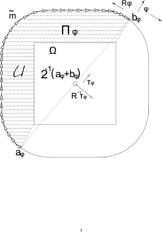
Let
, it is easy to see that
(52)
forms a connected set whose boundary is contained in and and in two lines parallel
to , see figure 2, also note the endpoints of
are given by and .
Figure 2.
Since either or so we can apply Lemma 1, to and thus there exists function such that
(53)
By the Co-area formula and Chebyshev’s inequality there exists
a set such that where
(54)
Pick .
Recall and define
(55)
We claim that
(56)
Since the endpoints of are the
same as the endpoints of it is sufficient to show
. Let
then let be the point given by
,
since is smooth , so
and thus
. As
this inequality is strict, in a neighborhood of the same
inequality will be satisfied. Thus we have
and so we have established (56).
By the construction of , and by (56) and
the choice of we have
(57)
There must exist
such that defining we have
(58)
Let . From the
construction it is clear that we can chose constant large enough so that
Let
(59)
For let
be the points defined by
and
.
By (57) we can assume constant was chosen large enough so that
. Let be the connected component
of that lies inside .
Thus
Note and
by definition of (see (55))
this together with (64) gives . Now if and so , it is imediate that
and so (again recalling
definition (55)) (50) follows.
On the other hand if then and so , ,
which implies so
hence (again recalling definition (55)),(50) also follows in this case.
Lemma 4.
Let be a convex body with . Let
be a function satisfying (7) and (8) and in addition
satisfies on and on in the sense of trace where is the
inward pointing unit normal to at .
Let be such that .
We will show there exists constant and such that
(65)
Proof of Lemma 4. Let be the convex set and be the function constructed in Lemma
3. To simplify our notation we will without loss of generality assume that .
It is easy to see we can chose such that , and . Without loss of
generality also assume . For any let denote the inward pointing
unit normal to at . Note that since otherwise
and this contradicts the fact that . For the same reason
.
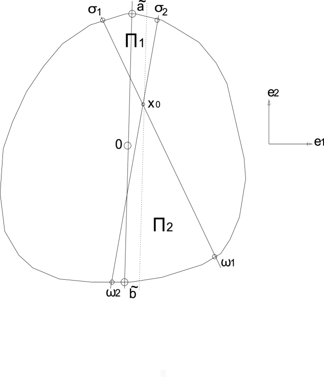
Step 1. Let be a
‘clockwise’ parameterisation of by arclength with . For
some
and we have that for
, , (see figure 3)
the points satisfy the following properties. Firstly
(66)
Secondly
(67)
Thirdly
(68)
Proof of Step 1. Recall , so for any
let be such that , note
that we can inscribe
a ball with and . Thus the curvature of is bounded
above by and so
(69)
Let be the set constructed in Lemma 3. We will show
(70)
Suppose this is not true, so for every ,
. Note that since is ,
is connected
and since , so
(71)
Note that as , and as generally for ,
so for any ,
(72)
So by the fundamental theorem of Calculus, . Now
Thus which is a contradiction. Thus we have established (70).
Hence (recalling the fact ) we can
pick such that
(73)
and . In the same way we can pick such that
and .
Define and . Since and recalling again that
,
Arguing in the same way we can establish . Thus as
is convex for which establishes
(66). Hence
which establishes (68) for . Inequality (68) for can be
established in the same way. Finally note
Step 2. For , , define
. We will show there exists positive constant and
such
that for some the following inequality holds
(75)
Proof of Step 2. Recall we know and are chosen
so that and . We also
know and . Let be the
unique point for which and let
be the
unique point for which , see figure 3.
Let us define for any , .
First we will show
however this inclusion is relatively easy to see because firstly
thus . And
secondly as
In exactly the same way . Hence
. Arguing in the same manner we have
and thus we have established the claim.
Let , by construction we have that lies in the component of
between and and hence by (74) we know
and so it follows
.
Since , and is convex we know and for
the same reasons see figure 3. So
and for exactly the same reason . Thus as and we have and
.
Hence
In other words the angle between and
is greater than
for some positive constant . Thus there exists
such that . Now
since we can apply Lemma 3 so we know that
Now for any we have
and .
Since from (66)
for we know and , from this it is easy to see (assuming
we chose large enough). And in the same way for any we also have
.
Step 3. There exists positive constant such that for some we have
(80)
where
(81)
Proof of Step 3. Let
. Note since is convex . We claim
(82)
Suppose this were not the case, then
. Since is convex (and recall ) and
we know
which
implies and thus
(83)
however as , and this is a contradiction, thus (82) is established.
Let
in the case where
let .
Since we know
. Note also
is a connected
subset of , so hence for every
, . So we can pick such that some point
satisfies
and
(84)
Now since , we know . Using
again the fact that (where is the parameterisation of ) it is easy to see
by the fundamental theorem of Calculus that (84) implies
Let so as (and since again
) so thus we must have , this gives (80).
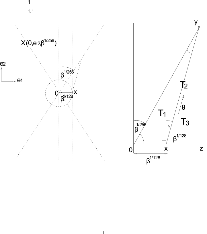
Step 4. We will show there exists a positive constant such that
(94)
Proof of Step 4. Without loss of generality we assume , and
. To begin with to take point
, we will show later the general case follows from this. See
figure 4.
Figure 4.
Let
and let
. We will get an upper bound on .
Let . We have two triangles to calculate with, triangle with corners on
which is a subset of triangle with corners on . Note that by applying the
law of sins we have .
Note that is also a right angle triangle and since
we have
.
Putting this together with the previous equation we have which gives
.
Now by taking the Taylor series approximating and we have
. Thus
and thus the existence of constant such that
(94) holds follows instantly for the case .
In the general case where suppose without loss of generality ,
define , since the angle between and
is with of it is easy to see
and of course so the
argument for the special case can be applied to show the
existence of constant satisfying (94).
Step 5. We will establish (65).
Proof of Step 5. Let
(95)
so we know .
So by the Fubini’s Theorem
(96)
Let
(97)
so we know ,
thus ,
assuming is small enough .
By Step 4, (94) for any
, we have
.
Since we can assume without loss
generality that . Pick , by the Co-area formula we must be able to find
such that
(98)
Let
. Let be
the endpoint of where we chose and . As already
noted, by Step 4 , so for any with by definition (95) we must have
so
(99)
Note also that if so and as
(recall from Step 2, and we
assumed without loss of generality )
(100)
thus
. Now for let denote the tangent
to , since so by the fundamental theorem of Calculus
(101)
Since the curvature of is bounded above by and by
(100) it is easy to see either is very close to or ,
we will without loss of generality assume the former, so by (100) we have
(102)
it is also easy to see and is -Lipschitz
on so
(103)
Note also as by (100) and the fact that and from Step 2 we know
, thus . Thus we have
(104)
Pick such that
. Now fix
, let and
denote a connected component of
.
So we know so we can apply the fundamental theorem of Calculus
we have that and since was an arbitrary point in
, using (104) this gives
(105)
By definition (see (44)) for any . Since putting this with (105) we have
(65).
Proof of Theorem 2. Let be a number
we obtain from Lemma 4 that satisfies (65). By Fubini’s Theorem we know
for some
constant .
Let
(106)
Note that .
Let be such that . Let .
Since we can
pick . So by the Co-area formula there exists
such that and
Let , we
can divide into disjoint pieces of equal length, denote them .
Formally; and for each . We can pick
for each .
Let
(112)
We define to be the convex hull of the points .
Now by the construction of , for any we can find such
that and thus and so
(113)
Note that by using (108) we know
and since (recalling also that is convex and so ) there exists positive constant such that
(114)
We claim
(115)
Suppose not, so there exists such that
.
By inequality (114) we know
and as by convexity of ,
thus
which contradicts the fact hence (115) is
established. Since the center of mass of is , i.e. , by (114), (115)
we have that .
Recall so so putting this together with (111) we have
(116)
Thus
(117)
Now using the elementary fact that , since we have
(118)
And thus
By Holder’s inequality this gives
(119)
Note that as and (113), (114) we established that so
.
Now for any
We begin by establishing the following proposition.
Proposition 1.
Let be a bounded convex domain with boundary
and there exists a
sequence such that
,
for (where is the inward
pointing unit normal to at ) and for which
Proof of Step 1. Suppose not, so we can pick . Let be an inward pointing unit normal to at , by convexity of
we have and so which implies which
contradicts that .
Step 2. .
Proof of Step 2. Suppose not. Since is convex we have and
thus we have which contradicts the fact that
.
Step 3. We will show .
Proof of Step 3. Suppose this implies
and
so which gives a contradiction.
Proof of Lemma completed. Suppose (123) is false, since we have
as before this implies which is a
contradiction.
Lemma 6.
Let be convex and define for any then
function is concave.
Proof of Lemma. Let . Since is convex
. Now suppose there exists
such that
then as this implies we must be able to find with
which is a contradiction.
Lemma 7.
Let , suppose is a convex set with .
Let . For any for which the approximate
derivative exists
(124)
Proof. For any let
be such that .
We begin by showing
(125)
Recall from Lemma 5
.
Using (122) from Lemma 5 and the fact
,
(126)
Hence
(127)
Therefor
Thus . Since we have
(128)
Hence
which gives
(129)
Let so using Lemma 5 and by (122) this easily implies
Since as putting this together
with (138) gives (135).
Step 2. We will show that for any
(139)
and
(140)
where denotes the total variation of measure .
Proof of Step 2. We can find such that .
Now from [Am-De 03] so in particular is a signed measure defined by
(141)
So for we have
Now given open set if then
So this in particular by Proposition 1.47 [Am-Fu-Pa 00] implies (140).
Now since we know by Theorem 3.78 [Am-Fu-Pa 00] that there exists a rectifiable set
(where denotes the set of approximate jump points of ) with and
where is the normal to the
approximate tangent of the rectifiable set at point . Following [Am-Fu-Pa 00] Definition 3.67 we assume
that the triple satisfies (3.69) of [Am-Fu-Pa 00]. By Theorem 3.94 [Am-Fu-Pa 00] we have
that is a rank- matrix for a.e. . Now
is a matrix valued measure and indeed letting denote the individual ‘component’ measures, just from the
definition we know that so is a symmetric matrix valued measure. Specifically
by differentiation of measures (see Theorem 2.2 [Am-Fu-Pa 00])
exists for a.e. and will be a symmetric matrix. So for a.e. ,
is a symmetric rank- matrix, this is easily seen to imply
. So
. Thus we can decompose into
absolutely continuous and singular parts we have
(142)
Obviously this is a matrix valued Radon measure and the signed Radon measure is given by the sum of diagonal elements of the
matrix defined by (142) and so is given by
Now recall for a.e. . So by Volpert chain rule (see Theorem 3.94 [Am-Fu-Pa 00])
we have that the function is BV and the standard chain rule holds so
(143)
Since we have
Letting denote the operator norm of a matrix, since
thus
Proof of Step 3. We define the ‘angle’ function by
(145)
Note that is smooth expect at the half line . For we
have , so as before
(146)
Since is the -Lipschitz,
(147)
and so from this and (134) we have that for any ,
and hence by (133)
is well defined along this level set.
We also know that for any the tangent to curve
is given by
.
Note that is the boundary of a smooth convex set so there
exists a point such that
. There
must also exist such that
(148)
Let denote the clockwise parameterization of by arc-length with . So . Define
by . Now pick
, suppose , then
Since (172) implies the diameter of is bounded by and since is a
convex set it follows immediately that .
Now the set equipped with the Euclidean norm is a boundly compact metric space. So by applying the
5r Covering Theorem (Theorem 2.1 [Ma 95]) we can find a disjoint collection of balls with such that . This
implies .
Since so and thus
which establishes (173).
As in Lemma 9 let
and
. Since is convex it is also a
set of finite perimeter. Let ,
it is clear . By
Theorem 3.83 [Am-Fu-Pa 00], . We know
by Lemma 9, . Now for any
, since
, . So
By Lemma 10 we know
that we can apply Theorem 1 of [Co-De 07] or Corollary 1.1 [Po 07] to find a
sequence that satisfies and for (where is the inward
pointing unit normal to at ) such that
In this section we will show that given a convex domain with boundary with curvature
bounded above by and that satisfies we will construct a
function with , this is the contents of Proposition 2 below.
The proof of Corollary 1 will follows easily from this.
Proposition 2.
Let be a convex body with boundary and with curvature
bounded above by and .
Let , there exists a function function
which satisfies (where is the inward
pointing unit normal to at ), for
and for which
Let be a continuous function. Let denote the standard convolution kernel,
i.e. and and define .
Suppose be an affine function, let then
(187)
Proof of Lemma. Let . As is affine
(188)
Lemma 12.
Let , suppose is a convex body with boundary and with curvature
bounded above by . Let . Let
be the standard convolution kernel and .
We will construct a function with on which satisfies the following properties
(189)
(190)
(191)
and
(192)
Proof. Let be a smooth monotonic function with the following properties
(193)
and .
For any define
(194)
We will
convolve the function with convolution kernel
. Since the convulsion
kernel varies with , when we differentiate , the derivative will involve a
term with the derivative of . For this reason we need to calculate various partial
derivatives of .
Since the curvature of is bounded above by
, for any we have that there is
one unique such that .
We define , let
and define .
Note , i.e. the inward pointing unit normal to at .
Note also that for all small enough , so . Thus
Note also that since and
so
Thus
(195)
So
(196)
and
(197)
Define
(198)
Now
(199)
In the same way it is easy to see and so
(200)
And
(201)
Finally
(202)
each term will be estimated later in Step 4.
Step 1. We will show
(203)
Proof of Step 1. Let be such that
. We start by showing
(204)
Now recall ,
. We have two cases to consider. Firstly the case that
. In this case since
is convex this implies . Thus as
so
(204) is established.
Now suppose we have the case that . Then let
(205)
Since the curvature of is bounded by we know that
. Consider the triangle whose corners are
, which we denote by . The
angle at corner is . Now since ,
, .
So as . Thus
Thus by the law of cosines
Which implies and so .
Let , since we
have . Consider the triangle . Note the
angle of this triangle at is and denoting the angle at by we have .
Then by the law of sins,
So which
gives . So as
and , (recalling the definition of from
(205)) . So
(204) is established. Thus letting we have that and this
completes the proof of Step 1.
Step 2. For any we have
(206)
Proof of Step 2. Since has curvature less than for any
, . So for any
, . Note as is convex
and so
.
Hence so it is clear that
(207)
For any we have where
is such that . So for any
by (207) we have that , so
.
Let be defined by , note by Lemma 11 we have
for any and hence
and as
Thus
(216)
So
(217)
Since we know
applying (217) and (212) to (210) gives
(218)
Now using that we have that
(219)
Thus and
(208) follows easily. Also for (218), (219) we know
and (209) follows.
This completes the proof of Step 3.
Step 4. We will show
(220)
Proof Step 4. We will estimate the terms in (202) one by one. First note
Note
and
(221)
So
(222)
From Step 2 (215) we know the existence of an affine function with
with .
Let so by Lemma 11 we know
. By following through the same calculation that gave (222) we have
Let be a convex domain and .
Let and define . Define
, we will
show that for any
(234)
Proof of Lemma. By the 5r Covering Theorem ([Ma 95], Theorem 2.1) them we can find a finite collection
of balls that are piecewise disjoint and
.
Note that for any since the set of ball in are pairwise disjoint, for some
constant there are at most balls from the set intersecting
. Thus and this obviously implies
.
For let .
Now given if , let
(235)
So
(236)
Now
(237)
Putting (237) together with (236) establishes (234).
Lemma 15.
Let , and define . Then
(238)
and
(239)
Proof of Lemma. Note for ,
(240)
So for
(241)
Since , for any
(242)
Hence
(243)
which establish. Now as and
for any so
Thus putting this together with (243) establishes (239).
Note so arguing in the same way as in (243) we have (238).
Let ,
let be the smooth monotonic function from the proof of Lemma 12,
so satisfies (193) and as in
Lemma 12 for
define
(244)
Let
(245)
and define
(246)
Let , and
define , note that
for any .
Recall from (198) the function defined in Lemma 12. Note that for any
function we defined by (244)
is identical to defined by (194) in Lemma 12. Hence as in
we have for any
thus
Since in , from (234) we have
and so putting this two inequalities together we have
(247)
Now as for any , and so
where and .
So and thus applying Lemma 15 we have
(248)
Since is Lipschitz, so is Lipschitz and so from (173) we have
(249)
And note for any
so
(250)
Putting these inequalities together we have
(251)
Now inequalities (247), (248) and (251) give us that satisfies
(186). And since on from (192)
satisfies for any . This completes the proof of Proposition
2.
Let . Let ,
note that since we can assume without loss of generality that so which gives
and so . Now we can also assume without loss of generality that . So
we can apply Proposition 2 which gives us the existence of such that(186) hold true. Hence we have
that . Let
be the minimiser of and since satisfies
and as
(252)
So we have that (7), (8) are satisfied
and hence by Theorem 2
Applying Lemma 7 we have
. So arguing is the same way as the proof of Corollary 2
we have .
References
[Al-Ri-Se 02] F. Alouges; T. Riviere; S. Serfaty. Neel and cross-tie wall energies for planar micromagnetic configurations. A tribute to J. L. Lions. ESAIM Control Optim. Calc. Var. 8 (2002), 31–68
[Am-De-Ma 99]
L. Ambrosio; C. De Lellis; C. Mantegazza, Line energies for gradient vector fields in the plane. Calc. Var. Partial Differential Equations 9 (1999), no. 4, 327–255.
[Am-De 03] L. Ambrosio; C. De Lellis, A note on admissible solutions of 1D scalar conservation laws and 2D Hamilton-Jacobi equations. J. Hyperbolic Differ. Equ. 1 (2004), no. 4, 813–826.
[Am-Fu-Pa 00] L. Ambrosio; N. Fusco; D. Pallara.
Functions of bounded variation and free discontinuity problems.
Oxford Mathematical Monographs. The Clarendon Press, Oxford
University Press, New York, 2000.
[Am-Le-Ri 03] L. Ambrosio; M. Lecumberry; T. Riviere A viscosity property of minimizing micromagnetic configurations. Comm. Pure Appl. Math. 56 (2003), no. 6, 681–688
[Am-Ki-Ri 02] L. Ambrosio; B. Kirchheim; M. Lecumberry; T. Riviere.
On the rectifiability of defect measures arising in a micromagnetics model. Nonlinear problems in mathematical
physics and related topics, II, 29–60, Int. Math. Ser. (N. Y.), 2, Kluwer/Plenum, New York, 2002.
[Av-Gi 87] P. Aviles; Y. Giga, A mathematical problem related to the physical theory of liquid crystal configurations. Miniconference on geometry and partial differential equations.
Proc. Centre Math. Anal. Austral. Nat. Univ., 12, Austral. Nat. Univ., Canberra, 1987.
[Av-Gi 96] P. Aviles; Y. Giga, On lower semicontinuity of a defect energy obtained by a
singular limit of the Ginzburg-Landau type energy for gradient fields. Proc. Roy. Soc.
Edinburgh Sect. A 129 (1999), no. 1, 1–17.
[Co-De 07] S. Conti; C. De Lellis. Sharp upper bounds for a variational problem with singular perturbation. Math. Ann. 338 (2007), no. 1, 119–146.
[De-Ot 03] C. De Lellis, F. Otto, Structure of entropy solutions to the eikonal equation. J. Eur. Math. Soc. (JEMS) 5 (2003), no. 2, 107–145.
[De-Ot-We 03] C. De Lellis, F. Otto, Felix; Westdickenberg, Michael Structure of entropy solutions for multi-dimensional scalar conservation laws. Arch. Ration. Mech. Anal. 170 (2003), no. 2, 137–184
[De-Ko-Mu-Ot 00] A. DeSimone; S. Muller, R. Kohn, F. Otto. A compactness result in the gradient theory of phase transitions. Proc. Roy. Soc. Edinburgh Sect. A 131 (2001), no. 4, 833–844.
[Di-Li-Me 91] R. DiPerna; P. Lions; Y. Meyer. regularity of velocity averages.
Ann. Inst. H. Poincaré Anal. Non Linéaire 8 (1991), no. 3-4, 271–287.
[Ev-Ga 92] L.C. Evans. R.F. Gariepy.
Measure theory and fine properties of functions. Studies in Advanced
Mathematics. CRC Press, Boca Raton, FL, 1992.
[Fed 69] H. Fededer. Geometric measure theory. Die Grundlehren der mathematischen Wissenschaften, Band 153 Springer-Verlag New York Inc., New York 1969.
[Fo-Ga 95] I. Fonseca, W. Gangbo. Degree theory in analysis and applications.
Oxford Lecture Series in Mathematics and its Applications, 2. Oxford
Science Publications. The Clarendon Press, Oxford University Press,
New York, 1995.
[Gi-Or 94] G. Gioia, M. Ortiz. The morphology and folding patterns of
buckling-driven thin-film blisters. J. Mech. Phys. Solids 42 (1994), no. 3, 531–559.
[Gi-Or 97] G. Gioia, M. Ortiz.
Delamination of compressed thin films. Adv. Appl. Mech. 33 (1997) 119-192.
[Ja-Pe 97] P. Jabin; B. Perthame.
Compactness in Ginzburg-Landau energy by kinetic averaging. Comm. Pure Appl. Math. 54
(2001), no. 9, 1096–1109.
[Ja-Ot-Pe 02] P. Jabin; F. Otto; B. Perthame.
Line-energy Ginzburg-Landau models: zero-energy states. Ann. Sc. Norm. Super. Pisa Cl. Sci. (5)
(2002), no. 1, 187–202.
[Ji-Ko 00] W. Jin, R.V. Kohn, Singular perturbation and the energy of folds.
J. Nonlinear Sci. 10 (2000), no. 3, 355–390.
[Le-Ri 02] M. Lecumberry; T. Riviere. Regularity for micromagnetic configurations having zero jump energy.
Calc. Var. Partial Differential Equations 15 (2002), no. 3, 389–402.
[Lo pr] A. Lorent. A Poincare type inequality for Aviles Giga energy and applications. Preprint.
[Ma 95] P. Mattila. Geometry of sets and measures in Euclidean spaces. Fractals and rectifiability. Cambridge Studies in Advanced Mathematics, 44. Cambridge University Press, Cambridge, 1995.
[Mo-Mo 00] L. Modica, S. Mortola. Un esempio di -convergenza.
Boll. Un. Mat. Ital. B (5) 14 (1977), no. 1, 285–299.
[Mu 78] F. Murat. Compacite par compensation: condition necessaire et suffisante de continuite faible sous une hypothese de rang constant. (French) Ann. Scuola Norm. Sup. Pisa Cl. Sci. (4) 8 (1981), no. 1, 69–102.
[Po 07] A. Poliakovsky. Upper bounds for singular perturbation problems involving gradient fields. J. Eur. Math. Soc. (JEMS) 9 (2007), no. 1, 1 43.
[Ri-Se 01] T. Rivière, S. Serfaty. Limiting domain wall energy for a problem related to micromagnetics.
Comm. Pure Appl. Math. 54 (2001), no. 3, 294–338.
[Ta 79] Tartar, L. Compensated compactness and applications to partial differential equations. Nonlinear analysis and mechanics: Heriot-Watt Symposium, Vol. IV, pp. 136–212, Res. Notes in Math., 39, Pitman, Boston, Mass.-London, 1979. 136-212.