Proceedings of the Workshop
on Monte Carlo’s, Physics
and Simulations at the LHC

PART II

Authors

F. Ambroglini ${}^{\ref{UniPG}}$, R. Armillis ${}^{\ref{Lecce}}$, P. Azzi ${}^{\ref{INFNPD}}$, G. Bagliesi ${}^{\ref{INFNPI}}$, A. Ballestrero ${}^{\ref{INFNTO}}$, G. Balossini ${}^{\ref{UniPV}}$, A. Banfi ${}^{\ref{UniMIB}}$, P. Bartalini ${}^{\ref{Taiwan}}$, D. Benedetti ${}^{\ref{Northeastern}}$, G. Bevilacqua ${}^{\ref{Demokritos}}$, S. Bolognesi ${}^{\ref{UniTO}}$, A. Cafarella ${}^{{\ref{Demokritos},\ref{Lecce}}}$, C.M. Carloni Calame ${}^{\ref{Southampton}}$, L. Carminati ${}^{\ref{UniMI}}$, M. Cobal ${}^{\ref{Udine}}$, G. Corcella ${}^{{\ref{FermiZ},\ref{Normale}}}$, C. Corianò ${}^{\ref{Lecce}}$, A. Dainese ${}^{\ref{Legnaro}}$, V. Del Duca ${}^{\ref{LNF}}$, F. Fabbri ${}^{\ref{INFNBO}}$, M. Fabbrichesi ${}^{\ref{INFNTS}}$, L. Fanò ${}^{\ref{INFNPG}}$, Alon E. Faraggi ${}^{\ref{Liverpool}}$, S. Frixione ${}^{{\ref{CERNTH},\ref{EPFL}}}$, L. Garbini ${}^{\ref{UniPG}}$, A. Giammanco ${}^{\ref{Louvain}}$, M. Grazzini ${}^{\ref{INFNFI}}$, M. Guzzi ${}^{\ref{Lecce}}$, N. Irges ${}^{\ref{Crete}}$, E. Maina ${}^{\ref{UniTO}}$, C. Mariotti ${}^{\ref{INFNTO}}$, G. Masetti ${}^{\ref{UniBO}}$, B. Mele ${}^{\ref{INFNRM1}}$, E. Migliore ${}^{\ref{UniTO}}$, G. Montagna ${}^{\ref{UniPV}}$, M. Monteno ${}^{\ref{INFNTO}}$, M. Moretti ${}^{\ref{Ferrara}}$, P. Nason ${}^{\ref{INFNMIB}}$, O. Nicrosini ${}^{\ref{INFNPV}}$, A. Nisati ${}^{\ref{INFNRM1}}$, A. Perrotta ${}^{\ref{INFNBO}}$, F. Piccinini ${}^{\ref{INFNPV}}$, G. Polesello ${}^{\ref{INFNPV}}$, D. Rebuzzi ${}^{\ref{INFNPV}}$, A. Rizzi ${}^{\ref{ETH}}$, S. Rolli ${}^{\ref{Tufts}}$, C. Roda ${}^{\ref{INFNPI}}$, S. Rosati ${}^{\ref{INFNRM1}}$, A. Santocchia ${}^{\ref{UniPG}}$, D. Stocco ${}^{{\ref{Subatech},\ref{UniTO}}}$, F. Tartarelli ${}^{\ref{UniMI}}$, R. Tenchini ${}^{\ref{INFNPI}}$, A. Tonero ${}^{\ref{SISSA}}$, M. Treccani ${}^{{\ref{granada},\ref{Ferrara}}}$, D. Treleani ${}^{\ref{UniTS}}$, A. Tricoli ${}^{\ref{Rutherford}}$, D. Trocino ${}^{\ref{UniTO}}$, L. Vecchi ${}^{\ref{SISSA}}$, A. Vicini ${}^{\ref{UniMI}}$, I. Vivarelli ${}^{\ref{INFNPI}}$.

1. University of Salento and INFN, Lecce, Italy

2. INFN, Frascati, Italy

3. University of Torino and INFN, Torino, Italy

4. INFN, Sezione di Torino, Torino, Italy

5. University of Milano Bicocca and Sezione INFN, Milano, Italy

6. University of Milano and Sezione INFN, Milano, Italy

7. University of Trieste and Sezione INFN, Trieste, Italy

8. University of Bologna and Sezione INFN, Bologna, Italy

9. INFN, Sezione di Bologna, Bologna, Italy

10. INFN, Sezione di Milano Bicocca, Milano, Italy

11. INFN, Sezione di Milano, Milano, Italy

12. INFN, Sezione di Roma, Roma, Italy

13. University of Pavia and INFN, Pavia, Italy

14. INFN, Sezione di Pavia, Pavia, Italy

15. INFN, Sezione di Trieste, Trieste, Italy

16. INFN, Sezione di Perugia, Perugia, Italy

17. SISSA/ISAS, Trieste, Italy

18. University of Ferrara and INFN, Ferrara, Italy

19. INFN, Sezione di Firenze, Firenze, Italy

20. University of Perugia and INFN, Perugia, Italy

21. INFN, Sezione di Padova, Padova, Italy

22. University of Padova and INFN, Padova, Italy

23. University of Pisa and INFN, Pisa, Italy

24. INFN, Sezione di Pisa, Pisa, Italy

25. Scuola Normale Superiore and INFN, Pisa, Italy

26. Department of Physics and Institute of Plasma Physics, University of Crete, Heraklion, Greece

27. National Taiwan University, Taipei, Taiwan.

28. INFN Gruppo Collegato di Udine, Udine, Italy

29. Museo Storico della Fisica e Centro Studi e Ricerche E. Fermi, Roma, Italy

30. INFN, Laboratori Nazionali di Legnaro, Padova, Italy

31. Institute of Nuclear Physics, NCSR “Demokritos”, Athens, Greece

32. Department of Mathematical Sciences, University of Liverpool, Liverpool, United Kingdom

33. Departamento de Física Teórica y del Cosmos, University of Granada, Granada, Spain

34. INFN and School of Physics and Astronomy, University of Southampton, Highfield, Southampton, UK

35. Subatech (Université de Nantes, Ecole des Mines and CNRS/IN2P3), Nantes, France

36. Northeastern University, Department of Physics, Boston, MA, USA

37. Université Catholique de Louvain, Louvain-la-Neuve, Belgium

38. Institute for Particle Physics, ETH Zurich, Zurich, Switzerland

39. Rutherford Appleton Laboratory, Science and Technology Facilities Council, Harwell Science and Innovation Campus, Didcot OX11 0QX, United Kingdom

40. PH Department, TH Unit, CERN, Geneva, Switzerland

41. ITPP, EPFL, Lausanne, Switzerland

42. INFN, Laboratori Nazionali di Frascati, Frascati, Italy

43. Tufts University, Medford, Massachusetts, USA

ALICE and its pp physics programme

M. Monteno for the ALICE Collaboration

1.1 Introduction

ALICE (A Large Ion Collider Experiment) is the dedicated heavy-ion experiment designed to measure the properties of the strongly interacting matter created in nucleus-nucleus interactions at the LHC energies ($\sqrt{s}=5.5$ TeV per nucleon pair for Pb–Pb collisions) [1, 2].

In addition, with its system of detectors, ALICE will also allow to perform interesting measurements during the proton–proton LHC runs at $\sqrt{s}=14$ TeV [3]. Special strength of ALICE is the low $p_{\scriptscriptstyle T}$ cut-off ($\sim$100 MeV/$c$) due to the low magnetic field, the small amount of material in the tracking detectors, and the excellent capabilities in particle identification over a large momentum range (up to $\sim$100 GeV/$c$). The above features of its conceptual design as soft-particle (low $p_{\scriptscriptstyle T}$) tracker make ALICE suitable to explore very effectively the global properties of minimum–bias proton–proton collisions (such as the distributions of charged tracks in multiplicity, pseudorapidity and transverse momentum) in the new domain of the LHC energies.

In addition, these measurements will provide also an indispensable complement to those performed in the other pp experiments, ATLAS and CMS, where the superposition of minimum-bias collisions at the highest LHC luminosity will be the main source of background to the search for rare signals (Higgs boson, SUSY particles, ’new physics’). On the other hand also the Underlying Event (i.e. the softer component accompanying a hard QCD process) must be carefully understood, since it accounts for a large fraction of the event activity in terms of the observed transverse energy or charged particle multiplicity and momenta.

Furthermore, as it will be shown in the following, the ALICE proton–proton programme will include also cross-section measurements of strange particles, baryons, resonances, heavy-flavoured mesons, heavy quarkonia, photons, and also jet studies.

Another motivation for studying pp events with ALICE is the necessity to provide a reference, in the same detector, to measurements performed with nucleus–nucleus (and proton–nucleus) collisions. The latter could be done via interpolation to $\sqrt{s}=5.5$ TeV (the centre-of-mass energy for Pb -Pb runs) between the Tevatron and the maximum LHC energy. However, since this interpolation will be affected by rather large uncertainties, additional dedicated runs at the same centre-of-mass energy as measured in heavy-ion collisions could be necessary to obtain a more reliable reference. Indeed, as it was shown by the past experiments at the SPS and at the RHIC, such comparison is important in order to disentangle genuine collective phenomena and to be more sensitive to any signatures of critical behaviour at the largest energy densities reached in head-on heavy-ion collisions.

Last, a more technical motivation of pp studies is that pp collisions are optimal for the commissioning of the detector, since most of the calibration and alignment tasks can be performed most efficiently with low multiplicity events.

For all the above reasons, from the Technical Proposal onwards the proton–proton programme has been considered an integral part of the ALICE experiment. This programme is going to be started at the commissioning of the LHC, which will happen with proton beams at low luminosities .

This review paper is organized as follows. After a section describing the ALICE detector, we will review the features of ALICE operations with pp collisions at the LHC, and the statistics and triggers required to accomplish its physics programme. Several physics topics will be addressed, but special emphasis will be given to the soft physics programme (event characterization, strange particle and resonance production, particle correlations, event-by-event fluctuations and baryon asymmetries measurements). Then, the ALICE capabilities in measuring some diffractive processes and its potentialities in the study of hard processes (jet and photon physics) will be presented, to conclude with some hints of possible studies of exotic processes (like mini black holes eventually produced by large extra dimensions).

The physics programme will include also measurements of heavy-flavoured mesons (open charm and beauty) and of quarkonia states, both in the central detector and in the forward muon spectrometer. However these studies will not be discussed here, since they are already reported in other contributions included in these proceedings ([4, 5]).

1.2 ALICE detector overview

ALICE, whose setup is shown in Fig. 1.1, is a general-purpose experiment whose detectors measure and identify mid-rapidity hadrons, leptons and photons produced in an interaction. A unique design, with very different optimisation than the one selected for the dedicated pp experiments at LHC, has been adopted for ALICE.

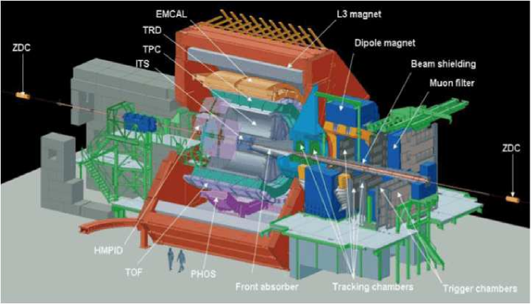
Figure 1.1: The ALICE experiment in its final layout.

This results from the requirements to track and identify particles from very low ($\sim$100 MeV/$c$) up to fairly high ($\sim$100 GeV/$c$) $p_{\scriptscriptstyle T}$, to reconstruct short-lived particles such as hyperons, D and B mesons, and to perform these tasks even in a heavy-ion collision environment, with large charged-particle multiplicities.

Theoretically founded predictions for the multiplicity in central Pb–Pb collisions at the LHC range at present from 1000 to 4000 charged particles per rapidity unit at mid-rapidity, while extrapolations from RHIC data point at values of about 1500. The ALICE detectors are designed to cope with multiplicities up to 8000 charged particles per rapidity unit, a value which ensures a comfortable safety margin.

The detection and identification of muons are performed with a dedicated spectrometer, including a large warm dipole magnet and covering a domain of large rapidities ($-4.0\leq\eta\leq-2.4$).

Hadrons, electrons and photons are detected and identified inside the central barrel, a complex system of detectors immersed in a moderate (0.5 T) magnetic field provided by the solenoid of the former L3 experiment.

Tracking of charged particles is performed by a set of four concentric detectors: the Inner Tracking System (ITS), consisting of six cylindrical layers of silicon detectors, a large-volume Time-Projection Chamber (TPC), a high-granularity Transition-Radiation Detector (TRD), and a high-resolution array of Multi-gap Resistive Plate Chambers (TOF). These detectors allow global reconstruction of particle momenta in the central pseudorapidity range $|\eta|<0.9$ (with good momentum resolution up to $p_{\scriptscriptstyle T}\sim 100$ GeV/c), and particle identification is performed by measuring energy loss in the ITS and in the TPC, transition radiation in the TRD, and time of flight with the TOF.

However, in the case of pp collisions, the lower particle density allows to increase the TPC acceptance by considering also tracks with only a partial path through the TPC, i.e. ending in the readout chambers; in that case the pseudorapidity coverage can be enlarged up to $|\eta|\leq 1.5$, with a lower momentum resolution.

Two additional detectors provide particle identification at central rapidity over a limited acceptance: the High-Momentum Particle Identification Detector (HMPID), that is an array of Ring Imaging Cherenkov counters dedicated to the identification of hadrons with $p_{\scriptscriptstyle T}>1$ GeV/c, and a crystal Photon Spectrometer (PHOS) to detect electromagnetic particles and provide photon and neutral meson identification.

Additional detectors located at large rapidities, on both sides of the central barrel, complete the central detection system to characterise the event on a wider rapidity range or to provide interaction triggers. The measurement of charged particle and photon multiplicity is performed respectively by the Forward Multiplicity Detector (FMD) (over the intervals $-3.4\leq\eta\leq-1.7$ and $1.7\leq\eta\leq 5.1$) and by the Photon Multiplicity Detector (PMD) (over the range $2.3\leq\eta\leq 3.5$). The V0 and T0 detectors, designed for triggering purposes, have an acceptance covering a rather narrow domain at large rapidities, whereas a set of four Zero-Degree Calorimeters (ZDC) will measure spectator nucleons in heavy-ion collisions and leading particles in pp collisions around beams’ rapidity.

Finally, in order to complete the ALICE capabilities in jet studies, a large lead-scintillator electromagnetic calorimeter (EMCal) [6, 7] will be located between the TOF and the L3 magnetic coils, adjacent to HMPID and opposite to PHOS. In its final configuration, the EMCal will have a central acceptance in pseudorapidity of $|\eta|<0.7$, with a coverage of $180\mbox{${}^{\circ}$}$ in azimuth, and an energy resolution of $\Delta E/E=10\%/\sqrt{E}$. It will be optimized for the detection of high-$p_{\scriptscriptstyle T}$ photons, neutral pions and electrons and, together with the central tracking detectors, it will improve the jet energy resolution.

The charged-particle multiplicity and the ${\mathrm{d}}N_{\mathrm{c}h}/{\mathrm{d}}\eta$ distribution will constitute the first basic observable which will be measured in ALICE, both for pp and Pb–Pb collisions at the LHC. In the central region the best performance in these measurements will be obtained with the Silicon Pixel Detector (SPD), the first two layers of the ITS, with approximate radii of 3.9 and 7.6 cm. A simple algorithm can be used in the SPD to measure multiplicity in a robust way by using ‘tracklets’, defined by the association of clusters of hits in two different SPD layers through a straight line pointing to the primary interaction vertex, assumed to be known [8]. The limits of the geometrical acceptance for an event with primary vertex at the center of the detector are $|\eta|<2$ for clusters measured on the first SPD layer and $|\eta|<1.5$ for tracklets measured with both SPD layers. However, the effective acceptance is larger, due to the longitudinal spread of the interaction vertex position, and its limits extend up to about $|\eta|<2$ for the multiplicity estimate with tracklets [9].

Therefore, by considering the partial overlap between the $\eta$ ranges covered by the SPD ($-2<\eta<2$) and by the FMD ($-3.4\leq\eta\leq-1.7$ and $1.7\leq\eta\leq 5.1$), it follows that the pseudorapidity range covered by the ALICE experiment for the charged-particle multiplicity and the ${\mathrm{d}}N_{\mathrm{c}h}/{\mathrm{d}}\eta$ measurements spans over about 8 pseudorapidity units.

1.3 ALICE operation with pp collisions

The proton–proton programme of ALICE will start already during the phase of commissioning of the LHC, when the luminosity will be low ($L<10^{29}$ cm^-2s^-1). This time will be a privileged period for ALICE to measure pp collisions, because there will be only a small pile-up in its slowest detectors and a low level of beam background [3].

However, when higher luminosities will be delivered by the LHC, a limiting factor for ALICE will be given by the readout of its detectors, essentially by the TPC, which is the slowest detector with its drift time of 88 $\mu$s, during which additional collisions may occur, causing several superimposed events (pile-up).

From the point of view of track reconstruction this would not be a problem, since the piled-up interactions in the TPC will keep a regular pattern with virtual vertices shifted along the drift direction. This can be tolerated, although at the price of heavier tracking and larger data volume for the same physics information, at least up to $L=3\times 10^{30}$ cm^-2s^-1.

At this luminosity the interaction rate amounts to about 200 kHz, assuming that the total inelastic pp cross section is 70 mb. The TPC records tracks from interactions which have occurred during the time interval 88 $\mu$s before and after the triggered bunch crossing. Hence on average 40 events will pile-up during the drift time of the TPC, before and after the trigger. However, on average only half of the tracks will be recorded, due to the fact that the other half will be emitted outside the acceptance. Therefore the total data volume will correspond only to the equivalent of 20 complete events. The charged-particle density at mid-rapidity in pp collisions at the nominal LHC centre-of-mass energy of $\sqrt{s}=14$ TeV is expected to be about 7 particles per unit of pseudorapidity, resulting in a total of $\sim$ 250(400) charged tracks within the TPC acceptance $|\eta|<0.9$ (or within the extended acceptance $|\eta|<1.5$, when including also tracks with only a short path through the TPC). Clearly, tracking under such pile-up conditions is still feasible, since the occupancy is more than an order of magnitude below the design value of the TPC.

For higher luminosity pile-up becomes progressively more difficult to handle, since events start to pile-up also in other detectors (silicon drift and silicon strip detectors, and then the HMPID). Therefore the luminosity $L=3\times 10^{30}$ cm^-2s^-1 is the maximum that can be tolerated, and in the following we will consider it as a benchmark for ALICE. When the LHC will reach its design luminosity ($L=10^{34}$ cm^-2s^-1) some strategies will be needed to record meaningful pp data by reducing the luminosity at the ALICE interaction point (e.g. beam defocussing and displacement).

For the benchmark luminosity $L=3\times 10^{30}$ cm^-2s^-1 the total pp event size (including pile-up and possible electronics noise) is estimated to be of the order of 2.5 MB, without any data compression. Thus, running at the foreseen maximum TPC rate of 1 kHz would lead to a total data rate of 2.5 GB/s. However, the online tracking of the High Level Trigger will select only tracks belonging to the interesting interaction. This pile-up suppression will reduce the event size by at least a factor 10.

According to current estimates of event sizes and trigger rates, a maximum data rate (bandwidth) of the Data Acquistion (DAQ) system of 1.25 GB/s to mass storage, consistent with the constraints imposed by technology, cost and storage capacity, would provide adequate statistics for the full physics programme. This will be possible by using a combination of increased trigger selectivity, data compression and partial readout.

The above needs of ALICE for data acquisition are well within the limits of bandwidth to mass storage provided by the central computing facility (TIER-0) of the LHC Computing GRID project, that will be installed at CERN.

1.4 Required statistics and triggers

An extensive soft hadronic physics programme will be feasible in ALICE using LHC proton beams since the machine commissioning phase, when the low luminosity will limit the experimental programme to the measurement of large-cross-section processes. This programme will include:

• event characterization, with the measurement of charged particle multiplicity, pseudorapidity and momentum spectra, and of the $\langle p_{\scriptscriptstyle T}\rangle$-multiplicity correlation;

• particle production measurements, i.e. yields and spectra of various identified particles, like strange particles ($\Lambda$, $\Xi$, $\Omega$, etc) and resonances (i.e. $\rho$, $K^{*}$ and $\Phi$), and baryon-antibaryon asymmetries;

• particle correlations (i.e HBT interferometry and forward-backward correlations) and event-by-event fluctuations.

The soft hadronic physics programme will rely on data samples of minimum-bias triggered events.

The statistics needed depends on the observable under study and spans the range from a few $10^{5}$ to a few $10^{8}$ events. For a multiplicity measurement, a few $10^{5}$ events will give a meaningful data sample; an order of magnitude more is needed for particle spectra; to study rare hadronic observables (e.g. $\Omega$ production) we will need a few times $10^{8}$ pp events. Therefore, a statistics of $10^{9}$ minimum-bias triggered events will fulfill the whole soft hadronic physics programme.

Since the readout rate of ALICE is limited to 1 kHz by the TPC gating frequency, the requirement is to be able to collect the data at the maximum possible rate: 1000 events/s, at an average of 100 events/s. In this way, at an average acquisition rate of 100 Hz, the required statistics can be collected during one typical year of operation ($10^{7}$ s)

However, at the same acquisition rate, a reasonable statistics for different physics topics can be collected already in the first few hours, days, or weeks of data taking. For example a few minutes will be sufficient to measure pseudorapidity density with $\sim 10^{4}$ events, while a few hours will allow to collect sufficient event statistics for multiplicity studies.

For all the above outlined soft physics programme ALICE will need a simple minimum-bias trigger for inelastic interactions, that will be provided by two of its sub-detectors: the Silicon Pixel Detector (the two innermost layers of the ITS), and the V0.

The basic building blocks of the Silicon Pixel Detector (SPD) are ladders, arranged in two concentric layers covering the central pseudorapidity region, and consisting of a 200 $\mu$m thick silicon sensor bump-bonded to 5 front-end chips. The signals produced by each chip are logically combined to form the global fast-OR (GLOB.FO) trigger element.

The V0 detector is composed of two independent arrays of fast scintillator counters located along the beam pipe on each side of the nominal interaction point and at forward/backward rapidities. Two different trigger elements are built with the logical combination of the signals from counters on the two sides: V0.OR requires at least one hit in one counter on one side, while V0.AND requires at least one hit in one counter on both sides.

The main background to minimum-bias events are beam–gas and beam–halo interactions. The rate of beam–gas collisions is expected to be much smaller than the rate of beam–halo collisions, whose magnitude should be of the same order as proton–proton collisions. It has been shown that the structure of beam–halo events is similar to that of beam–gas events, the difference being that beam–halo events happen at greater distances to the nominal interaction point (more than 20 m).

The proposed proton–proton minimum bias triggers, that use logical combinations of the above outlined trigger elements, result to be sensitive to interactions corresponding to $\sim 90$ % of the total inelastic cross section (and $\sim 99$ % of the non-diffractive cross section), and still reject the majority of beam–gas interactions [10].

On the other hand the SPD global fast-OR (GLOB.FO) trigger element can also be used to provide a high multiplicity trigger, that will allow to collect enriched statistics in the tail of multiplicity distributions.

As regards the other physics topics (open heavy flavour mesons and quarkonia production; diffractive processes studies; jet and photon physics) they require separate high statistics data samples that would need high rates and bandwidth. Dedicated trigger and HLT algorithms will significantly improve the event selection and data reduction, and will allow to collect data samples of adequate statistics already in one year of data taking.

Some details on triggers for diffractive processes and jets will be given in following dedicated sections.

1.5 Event characterization

For the first physics measurements, shortly after the LHC start-up, in order to minimize the uncertainty stemming from non-optimal alignment and calibration, a few detectors systems will be sufficient: the two inner layers of the ITS (the Silicon Pixel Detector), the TPC, and the minimum-bias trigger detectors (V0 and T0). Indeed, particle identification will have a limited scope during initial runs, since it requires a precise calibration and a very good understanding of the detectors. Four measurements of soft hadronic physics which can be addressed during the first days of data taking will be outlined in this section: 1) the pseudorapidity density of primary charged particles, 2) the charged particle multiplicity distribution, 3) transverse momentum spectra and 4) the correlation of $\langle p_{\scriptscriptstyle T}\rangle$ with multiplicity.

These measurements of global event properties will be discussed in the context of previous collider measurements at lower energies and of their theoretical interpretations.

1.5.1 Pseudorapidity density

The pseudorapidity density of primary charged particles at mid-rapidity ${{\mathrm{d}}N_{\mathrm{c}h}/{\mathrm{d}}\eta|}_{\eta\approx 0}=1/\sigma^{inel}\cdot({\mathrm{d}}\sigma_{\mathrm{c}h}/{\mathrm{d}}\eta)_{\eta\approx 0}$ has been traditionally among the first measurements performed by experiments exploring a new energy domain. Indeed this measurement is important since it gives general indications on the interplay between hard and soft processes in the overall particle production mechanisms, and furthermore it brings important information for the tuning of Monte Carlo models. A simple scaling law ($\sim\ln s$) for the energy dependence of particle production at mid-rapidity was predicted by Feynman [11], but it appeared clearly broken in collisions at the SPS [12, 13]. Indeed, the best fit to the pp and $\mathrm{p}$$\bar{\mathrm{p}}$ data, including that from SPS and Tevatron colliders [14], follows a ln${}^{2}s$ dependence, whose extrapolation at $\sqrt{s}$=14 TeV gives about 6 particles per rapidity unit for non-single diffractive interactions.

A reasonable description of the energy dependence of the charged particle density is obtained within the framework of the Quark Gluon String Model (QGSM) [15], a phenomenological model that makes use of very few parameters to describe high-energy hadronic interactions. In this model, based on the ideas of Regge theory, the inclusive cross sections ${\mathrm{d}}\sigma_{\mathrm{c}h}/{\mathrm{d}}\eta$ increase at very high energies and at $\eta\approx 0$ as a power-law $\sim({s/s_{0}})^{\Delta}$, where $s_{0}=1$ GeV² and $\Delta=\alpha_{P}-1$ is related to the intercept $\alpha_{P}$ of a Pomeron (Regge) trajectory. Indeed, with the value $\alpha_{P}=0.12\pm 0.02$ found from the analysis of $\sigma^{tot}(s)$ [16] it results that the QGSM model reproduces successfully the observed growth of pseudorapidity distributions with energy [17].

Furthermore, the increase with energy of the charged particle density as well as the bulk properties of minimum bias events and of underlying event in hard processes are successfully reproduced (up to Tevatron energy) by models assuming the occurrence of multiple parton interactions in the same pp collision [18, 19, 20]. Examples of such models, extending the QCD perturbative picture to the soft regime, are implemented in the general purpose Monte Carlo programmes PYTHIA [21], JIMMY [22], SHERPA [23] and HERWIG++ [24], all of them containing several parameters that must be tuned by comparison against available experimental data. On the other hand, another successful description of the available data is provided by the Monte Carlo model PHOJET [25] which is based on both perturbative QCD and Dual Parton Model. However, the growth of particle density predicted by PHOJET is slower than in multiple parton interaction models, and so the charged particle density at LHC energy results to be $\sim$ 30% smaller.

ALICE will measure the ${\mathrm{d}}N_{\mathrm{c}h}/{\mathrm{d}}\eta$ distribution around mid-rapidity by counting correlated clusters (tracklets) in the two layers of the SPD (${|{\eta}|<2}$), and/or by counting tracks in the TPC (up to ${|{\eta}|=1.5}$). At the low multiplicity typical for proton–proton events, the occupancy in the highly segmented detectors will be very low, and corrections for geometrical acceptance, detector inefficiency and background contamination (from secondary interactions and feed-down decays) will be applied on track level. A second correction, taking into account the bias introduced by the vertex reconstruction inefficiency, will be applied on a event-by-event level (see Ref.[26] for more details).

The measurement can be done with very few events ($10^{4}$ events will give a statistical error of  $\sim$ 2 % for bins of $\Delta\eta=0.2$, assuming ${{\mathrm{d}}N_{\mathrm{c}h}/{\mathrm{d}}\eta|}_{\eta\approx 0}=6$).

In addition, the measurement of the pseudorapidity distribution can also be performed in the forward region (on the pseudorapidity intervals $-3.4\leq\eta\leq-1.7$ and $1.7\leq\eta\leq 5.1$), with the Forward Multiplicity Detector, but a complete understanding of secondary processes, which are dominant at low angles, is required.

1.5.2 Multiplicity distribution

The multiplicity distribution is the probability $P_{n}$ to produce $n$ primary charged particles in a collision.

At energies below $\sqrt{s}$=63 GeV (up to the ISR domain), the multiplicity distributions still scale with the mean multiplicity [27], following an universal function ($P_{n}=\langle n\rangle^{-1}\Phi(n/<n>)$)[28]. For higher energies, starting from the SPS, the KNO-scaling appears clearly broken [29]. The peculiarities of the measured multiplicity distributions (as the shoulder structure in their shape) have been explained in a multi-component scenario, by assuming an increased contribution to particle production from hard processes (jets and minijets). Multiplicity distributions are fitted to a weighted superposition of negative binomial distributions corresponding to different classes of events (soft and semi-hard) [30, 31, 32]. In alternative approaches, the violation of the KNO-scaling is understood as an effect of the occurrence of multiple parton interactions [33], or in terms of multi-Pomeron exchanges [34].

However, the general behaviour of multiplicity distributions in pp collisions in full phase space is quite uncertain. For example data at $\sqrt{s}$=546 GeV from E735 and UA5 differ by more than a factor of two above $N_{\mathrm{c}h}\approx 80$ [35]. Therefore extrapolations to higher energies or to full phase space of distributions measured within limited rapidity intervals are affected by rather big inaccuracies.

Experimentally the multiplicity distribution is not straightforward to extract. The detector response matrix, i.e. the probability that a certain true multiplicity gives a certain measured multiplicity, can be obtained from detector simulation studies. Using this, the true multiplicity spectrum can be estimated from the measured spectrum using different unfolding techniques [36, 37, 38]. The procedure of measuring the multiplicity distribution with the ALICE detector (using the Silicon Pixel Detector of the ITS, as well as the full tracking based on the TPC), is thoroughly described in Ref.[39]

ALICE reach in multiplicity with the statistics foreseen for the first physics run ($\geq 10^{7}$ minimum-bias triggered events) is about 125 ($|\eta|<0.9$). However, a large statistics of high-multiplicity events, with charged-particle rapidity densities at mid-rapidity in the range $60$–$70$ (i.e.  ten times the mean multiplicity) can be collected by using a high-multiplicity trigger based on the SPD Fast-OR trigger circuit. This class of events may give access to initial states where new physics such as high-density effects and saturation phenomena set in.

Also, local fluctuations of multiplicity distributions in momentum space and related scaling properties (intermittent behaviour) might be a possible signature of a phase transition to QGP[40]. This makes it interesting to study such multiplicity fluctuations in pp collisions.

1.5.3 Transverse momentum spectra

Collider data on charged-particle $p_{\scriptscriptstyle T}$ spectra have shown that the high $p_{\scriptscriptstyle T}$ yield rises dramatically with the collision energy, due to the increase of the hard processes cross sections [41].

At high $p_{\scriptscriptstyle T}$ the transverse momentum spectra are well described by LO or NLO pQCD calculations, but involving several phenomenological parameters and functions (K-factor, parton distribution functions and fragmentation functions) which need an experimental input to be determined. At lower $p_{\scriptscriptstyle T}$, where perturbative QCD calculations cannot be performed, theoretical foundations of different models are even more insecure. Therefore, early measurements of $p_{\scriptscriptstyle T}$ spectrum are important for the tuning of the model parameters and for the understanding of the background in the experimental study of rare processes. Also, the measurement of the $p_{\scriptscriptstyle T}$ spectrum is important to perform high-$p_{\scriptscriptstyle T}$ hadron suppression studies in in heavy-ion collisions, where the proton–proton data is used as reference.

In ALICE the track reconstruction is performed within the pseudorapidity interval $|\eta|<0.9$ through several steps (see section 5.1.2 of Ref. [2] for a detailed description of the procedure). Firstly, track finding and fitting in the TPC are performed from outside inward by means of a Kalman filtering algorithm [42]. In the next step, tracks reconstructed in the TPC are matched to the outermost ITS layer and followed in the ITS down to the innermost pixel layer. As a last step, reconstructed tracks can be back-propagated outward in the ITS and in the TPC up to the TRD innermost layer and then followed in the six TRD layers, in order to improve the momentum resolution.

As it was already said before, the TPC acceptance covers the pseudorapidity region $|\eta|<0.9$, but this range can be extended up to $|\eta|\simeq 1.5$ when analyzing tracks with reduced track length and momentum resolution.

The $p_{\scriptscriptstyle T}$ spectrum is measured by counting the number of tracks in each $p_{\scriptscriptstyle T}$ bin and then correcting for the detector and reconstruction inefficiencies (as a function of $z$, $\eta$ and $p_{\scriptscriptstyle T}$). Finally, the $p_{\scriptscriptstyle T}$ distribution is normalized to the number of collisions and corrected for the effect of vertex reconstruction inefficiency and trigger bias.

With an event sample of $\geq 10^{7}$ event that could be collected in the first runs ALICE could reach $p_{\scriptscriptstyle T}>40$ GeV/c.

1.5.4 Mean transverse momentum versus multiplicity

The correlation between charged-track $\langle p_{\scriptscriptstyle T}\rangle$ and multiplicity, describing the balance between particle production and transverse energy, is known since its first observation by UA1 [43], and it has been successively studied at the ISR [44] and Tevatron [45, 46] energies. The increase of $\langle p_{\scriptscriptstyle T}\rangle$ as a function of multiplicity has been also suggested by cosmic ray measurements [47].

This correlation between $\langle p_{\scriptscriptstyle T}\rangle$ and multiplicity is generally attributed to the onset of gluon radiation, and explained in terms of the jet and minijet production increasing with energy [48]. However, CDF data [46] have shown that the rise of the mean $p_{\scriptscriptstyle T}$ with multiplicity is also present in events with no jets (soft events). This behaviour is not yet satisfactorily explained by any models or Monte Carlo generators (as PYTHIA [21] and HERWIG [49]).

In ALICE it will be relatively straightforward to obtain the correlation between the mean $p_{\scriptscriptstyle T}$ and the charged particle multiplicity, once the multiplicity distribution and the $p_{\scriptscriptstyle T}$ spectra have been measured. The $p_{\scriptscriptstyle T}$ cut-off imposed by the detector ($\sim$ 100 MeV/c for pions and $\sim$ 300 MeV/c for protons) introduces a rather large systematic uncertainty on the $\langle p_{\scriptscriptstyle T}\rangle$ estimate.

Detailed measurements of the $\langle p_{\scriptscriptstyle T}\rangle$ versus multiplicity (eventually in different regions in $\eta$-$\phi$ relative to leading-jet direction, as in CDF analyses [50]) will give an insight to jet fragmentation processes and to the general Underlying Event structure.

Another interesting subject for ALICE, due to its powerful particle identification system at low and high $p_{\scriptscriptstyle T}$, will be the correlation between $\langle p_{\scriptscriptstyle T}\rangle$ and multiplicity studied separately for pions, kaons and proton/antiprotons. The data collected at Tevatron by the E735 experiment [45] indicate that the correlation has rather different behaviour for the three types of particles, especially as regards the proton and antiproton $\langle p_{\scriptscriptstyle T}\rangle$, that do not appear to saturate at high multiplicity as pions (and maybe also kaons, within experimental uncertainties). This is not yet understood in terms of the available hadronic models.

1.6 Strange particle measurements

There are basically two main motivations for ALICE to measure strange particle production in pp collisions at the LHC centre-of-mass energy of 14 TeV: 1) extending the range where strange quark production has been probed in pp collisions; 2) providing a reference for the measurement of strangeness production in heavy ion collisions, in view of the strangeness enhancement which was observed to set in at the SPS centre-of-mass energy ($\sqrt{s_{\mathrm{NN}}}=17$ GeV).

Strange and light quark production rates are usually compared by means of several observables. The most simple ones are measured particle ratios, like the widespreadly used $K/\pi$, that features a slight and remarkably stable increase in pp and $\mathrm{p\overline{p}}$ collisions, between $\sqrt{s}=27$ and 1800 GeV.

However, ideally one would like to extract directly from data the ratio between newly produced $s$ and $u$, $d$ quarks at hadronization, before hadronic decays take place. A useful way to measure such strangeness content is the so-called “Wroblewski ratio”, defined as: $\lambda_{S}=\frac{2s\bar{s}}{u\bar{u}+d\bar{d}}$. The earliest attempts to determine $\lambda_{S}$ were done in [51], on the basis of the models in Refs. [52]. In pp collisions and in the $\sqrt{s}$ range from 10 GeV to 900 GeV a fairly constant value of $\lambda_{\mathrm{s}}\sim 0.2$ has been extracted from the data (see Fig. 1.2) and there is no evidence of a rise [53] with increasing energy. This figure also summarizes the results from heavy-ion collisions.

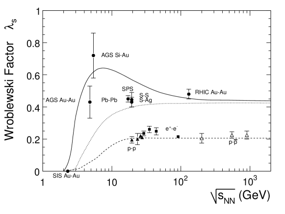
Figure 1.2: The Wroblewski factor $\lambda_{\mathrm{s}}$ as a function of $\sqrt{s}$.

On the other hand, more recent analyses based on statistical models of hadronization [54] have had great success in describing experimental data. This is shown in Fig. 1.2 by the dashed line, which comes from a canonical description using a correlation volume of two protons. This correlation volume causes a strangeness reduction as compared to heavy-ion collisions, which have a $\lambda_{\mathrm{s}}$ around 0.43.

In the case of heavy-ion collisions the parameter of the statistical models are interpreted thermodynamically, ascribing a “temperature” and some “thermodynamic potentials” to the system. However, it remains unclear as to how such models can successfully describe particle production in systems of small volume like those occurring during pp collisions. On the other hand it must be remarked that a pp system does not have to be thermal on a macroscopic scale to follow statistical emission. The apparently statistical nature of particle production observed in pp data could be simply a reflection of the statistical features of underlying jet fragmentation, or a result of phase space dominance considerations.

From Fig. 1.2 one might conclude that the strangeness content in elementary collisions will hardly increase with incident energy. However, this is far from being clear. The number of produced particles in pp collisions will increase up to values similar to those observed in heavy-ion collisions at the SPS. Hence, the volume parameter in the canonical description may have to be increased to account for the higher multiplicity. This would result in an increasing strangeness content.

Furthermore, at the LHC energies, the dominance of jet and minijet production will raise new questions since the final hadronic yields will originate from two different sources: a source reflecting the equilibrated (grand) canonical ensemble (soft physics) and on the other hand the fragmentation of jets (hard physics), that differs from the behavior of an equilibrated ensemble. By triggering on events with one, two or more jets, a ‘chemical analysis’ of these collisions will be possible. This very new opportunity would allow us to study whether the occurrence of hard processes influences the Underlying Event distributions. Particularly interesting in this context is the behaviour of strange and multi-strange particles, e.g. the K/$\pi$ or $\Omega/\pi$ ratio, in combination with extremely hard processes.

Possible effects of strangeness enhancement might be amplified when selecting events with high multiplicity. In this respect ALICE, thanks to the high-multiplicity trigger provided by the Silicon Pixel Detector can collect samples enriched in high multiplicity events, and so it will reach multiplicities 10 times the mean multiplicity. This study has gained special interest recently, when arguments for ‘deconfinement’ have been advocated in $\rm{\bar{p}}p$ collisions at Tevatron energies [55].

Moreover, several kinematical properties of strange particle production, like the multiplicity density dependence of their yield and their $p_{\scriptscriptstyle T}$ spectra, have been measured in the past, up to Tevatron energies, and still await a full theoretical explanation. For example the $K^{0}_{S}$ and $\Lambda$ $p_{\scriptscriptstyle T}$ spectra recently measured with high statistics and rather large $p_{\scriptscriptstyle T}$ coverage by the STAR experiment [56] in $\sqrt{s}=200$ GeV pp collisions at the RHIC collider have been compared to NLO pQCD calculations with varied factorization scales and fragmentation functions (taken from [57] for $K^{0}_{S}$ and from [58] for $\Lambda$). Although for the $K^{0}_{S}$ a reasonable agreement is achieved between the STAR data and the NLO pQCD calculations, the comparison is much less favorable for the $\Lambda$. A better agreement is obtained by Albino, Kniehl and Kramer in [59] when using a new set of fragmentation functions constrained by light-quark flavour-tagged $e^{+}e^{-}$ data from the OPAL experiment [60]. It will prove helpful to perform similar comparisons at LHC energies.

It was shown by the E735 Collaboration at Tevatron [61] that kaons $\langle p_{\scriptscriptstyle T}\rangle$ has stronger correlations with the charge multiplicity per unit rapidity than the pions $\langle p_{\scriptscriptstyle T}\rangle$: while the latter shows a saturation at $\langle dN/d\eta\rangle\approx 10$, the former continues to grow, although slightly decreasing its slope; the same behaviour is seen for antiprotons. Since $\langle dN/d\eta\rangle$ can be related to the energy density or entropy density [62], this behaviour is certainly relevant for quark-gluon plasma searches, besides providing constraints on models attempting to describe hadron production processes. ALICE can test this behaviour at much higher multiplicity densities and for other identified mesons and baryons carrying strangeness quantum numbers.

Finally, the measurement of higher resonances in pp will be important to obtain the respective population. This can be useful as input for the statistical models, but also for comparison with what is found in heavy-ion collisions, though in the latter case the yields are likely to be changed by the destruction of the resonances following the rescattering in the medium.

For all the reasons discussed above it appears very important to measure strange particles over a broad range of transverse momentum in the new regime of LHC energy. The ALICE experiment will face this challenge, for both pp and Pb–Pb collisions, thanks to the large acceptance and high precision of its tracking apparatus and particle identification methods.

Strange particle can be identified over a wide range in $p_{\scriptscriptstyle T}$ from the topology of their decays (“kinks” for charged kaons and secondary vertices for $K^{0}_{S}$, $\Lambda$, $\Xi$ and $\Omega$ decays) or otherwise from invariant mass analyses (for resonance decays).

The decay pattern of charged kaons into the muonic channel, with one charged daughter track (a muon) and one neutral daughter (a $\nu_{\mu}$) which is not observable in the tracking detectors, is known as a “kink”, as the track of the charged parent (the $K^{\pm}$ candidate) appears to have a discontinuity at the point of the parent decay. The kink-finding software loops on all charged tracks by applying to them some cuts to look for pairs of tracks compatible with the kink topology described above. The reconstruction of the kink topology is a key technique for identifying charged kaons over a momentum range much wider than that achieved by combining signals from different detectors (ITS, TPC, TOF and HMPID). Simulation studies have shown that for a total sample of $10^{9}$ pp events, in a full year of pp data taking at the LHC, a usable statistics of kaons can be obtained up to 14 GeV/c. However, when exploiting the relativistic rise of the energy loss signal in the TPC, the momentum reach can be further on enlarged up to 50 GeV/c.

Strange particles as $K^{0}_{S}$, $\Lambda$, $\Xi$ and $\Omega$ decay via weak interactions a few centimeters away from the primary vertex, and therefore they can be identified by using topological selections.

In the case of $K^{0}_{S}$ and $\Lambda$ the dominant decay channels are $K^{0}_{S}\rightarrow\pi^{+}\pi^{-}$ and $\Lambda\rightarrow p\pi^{-}$. The charged tracks of the daughter particles form a characteristic V-shaped pattern known as a “V0”, whose identification is performed by pairing oppositely charged particle tracks to form V0 candidates. Then, a set of geometrical cuts is applied, for example to the distance of closest approach (DCA) between the daughter track candidates and to the V0 pointing angle, in order to reduce the background and to maximize the signal-to-noise ratio. More efficient algorithms for V0 reconstruction, named “on-the-fly”, i.e. performed during track finding, are also under study.

The identification of the so-called “cascades” ($\Xi^{-}\rightarrow\Lambda\pi^{-}$ and $\Omega^{-}\rightarrow\Lambda K^{-}$), goes through pairing V0 candidates with a single charged track, referred to as the “bachelor”, and then using selections on the V0 mass and impact parameter, the DCA between the V0 and the bachelor, the bachelor impact parameter and the cascade pointing angle.

The reconstruction of secondary vertices (that has been thoroughly investigated in section 6.2 of [2]), relies on the primary vertex reconstruction. ALICE shows good performances for the identification of secondary vertices from strange hadrons decays, both in Pb–Pb and pp collisions. In the latter case particle multiplicities are low, and combinatorial background is even lower, so that topological cuts can be loosened in order to gather more signal. However, the reconstruction of the primary vertex position in the low-multiplicity events produced by pp collisions is affected by a large error, which substantially alter the reconstruction efficiency.

In any case a clear signal is obtained, as can bee seen in Fig.1.3 that shows in the left panel, for the case of the $\Lambda$ reconstruction, the signal and background invariant mass spectra obtained for pp events generated with PYTHIA 6.214. The right panel shows the estimated distribution of reconstructed $\Lambda$ versus $p_{\scriptscriptstyle T}$ in the central rapidity range $|y|<0.8$, for one year of LHC running ($10^{9}$ events).

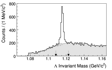
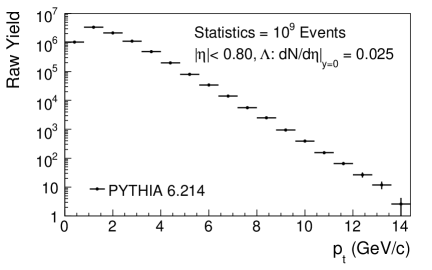
Figure 1.3: Invariant mass distributions of $\Lambda$ reconstructed in pp events for tight selections (left); distribution of reconstructed $\Lambda$ as a function of $p_{\scriptscriptstyle T}$ for $10^{9}$ pp events at $\sqrt{s}=14$ TeV (right).

Therefore the simulation (presented in [2] and in [63]) shows that transverse mass spectra for $\Lambda$ should be measurable up to $\sim 11$ GeV/c in a full year of pp data taking at the LHC. On the other hand the maximum $p_{\scriptscriptstyle T}$ reachable for $K^{0}_{S}$ and the multi-strange hyperons $\Xi$ and $\Omega$ are 12, 8 and 7 GeV/c respectively.

It must be remarked that in all the topological methods described above the single particle identification is not required, which makes them especially efficient at intermediate and high $p_{\scriptscriptstyle T}$, where particle identification based on energy loss (in ITS or TPC) and time-of-flight (in TOF) measurement fail. Therefore these studies can be performed by using only the basic ALICE tracking devices (the TPC and the ITS).

As regards strange resonance identification, as for example the $K^{*}(892)$ and the $\Phi(1020)$ since they decay very early, their daughters are not discernible from other primary particles.

Their main decay modes are $K^{*}\rightarrow K^{+}\pi^{-}$ and $\Phi\rightarrow K^{+}K^{-}$. Therefore these resonances are identified via invariant mass reconstruction methods that combine all possible pairs of primary daughter candidates. The background is very high since no selection other than particle identification or track quality is applied, and can be accurately estimated by means of ’like-sign’ or ’event mixing’ procedures. The kaon and pion identification is obtained from the energy loss in the TPC and from the time-of-flight measured in the TOF.

It has been found by preliminary analyses that for both resonances reaching $p_{\scriptscriptstyle T}$ as high as 4 GeV/c is not problematic. However, the identification of higher-$p_{\scriptscriptstyle T}$ resonances should be done without using particle identification.

All the tools to identify strange secondary vertices and resonances will provide first-physics observables, and a rather large statistics can be detected within the very first hours of LHC run. However, within a larger time scale (like the first full year of pp LHC run), the statistics of strange particles reconstructed with ALICE will by far overstep that of the previous pp and $\mathrm{p\overline{p}}$ experiments, and will allow several new studies that were barely achievable up to now because of statistics, such as the properties of $p_{\scriptscriptstyle T}$ spectra in a range of $p_{\scriptscriptstyle T}$ covering soft, intermediate and hard regimes, as wide as possible to understand the underlying QCD processes; and to be compared with the phenomena observed in nucleus–nucleus collisions at comparable centre-of-mass energy.

1.7 Baryon measurements

Studies of baryon production in the central rapidity region of high energy pp collisions provide a crucial possibility to test the baryon structure and to establish how the baryon number is distributed among the baryon constituents: valence quarks and sea quarks and gluons.

Hadronic processes are described by several models (DPM[64], QGSM [15], PYTHIA [21]) in terms of color strings stretched between the constituents of the colliding hadrons. In the framework of such models the dominant contribution to particle production in pp collisions involves diquark–quark string excitations followed by string breaking. The unbroken diquark system, playing the role of carrier of baryon number, will take large part of the original proton momentum and subsequently fragment into leading baryons, concentrated in the fragmentation region of the colliding protons. Such approach, where baryon number transfer over wide rapidity intervals is strongly suppressed, describes successfully the bulk of data on leading baryon production.

However, the observed high yield of protons in central rapidity region observed in experiments at the ISR pp collider (in the energy interval $\sqrt{s}=23-63$ GeV), cannot be explained in the framework of such models, that assume an indivisible diquark. These measurements indicate that the baryon number can be transported with high probability over a rather large rapidity gap ($\Delta y\leq$ 4)[65]. An appreciable baryon stopping is observed, with baryons exceeding antibaryons, and in association with higher hadron multiplicities.

To describe such data other mechanisms of baryon number transfer have been suggested, following the approach originally introduced by Rossi and Veneziano [66]. They have shown how it is possible to generalize to baryons the successful schemes employed to unify gauge, dual and Regge-Gribov theories of mesons. Their results on the topological structure of diagrams of processes involving baryons can be rephrased in a dual string picture in which the baryon (for $N_{c}=3$) is a Y-shaped object with valence quarks sitting at the ends and with a string junction in the middle. Then, it can be assumed that the baryon number is carried by valence quarks, or otherwise by the string junction itself, which is a non-perturbative configuration of gluon fields.

In a first approach [67] the baryon number of the incident proton is assumed to be transferred to a more central rapidity region through a mechanism by which a valence quark is slowed down to the central rapidity region, while a fast spectator diquark is destroyed. The cross section of the baryon number flow has been estimated using perturbative QCD calculations: it has been found to depend on the rapidity gap $\Delta\mathrm{y}$ approximately as $\exp^{-\Delta\mathrm{y}}$ and nicely agrees with the data at ISR energies. Another estimate [68], based on the topological approach and Regge phenomenology, and considering also the stopping of string junctions in the central rapidity region, finds a similar dependence of single baryon stopping cross section on energy and rapidity, in agreement with the ISR data.

In an alternative approach [69] the baryon number is assumed to be transferred dominantly by gluons. This mechanism does not attenuate baryon number transfer over large rapidity gaps, since the transfer probability is independent of rapidity.

The HERA data on high-energy photon-proton collisions have offered a unique opportunity to study the mechanisms of baryon number transfer. The asymmetry in the e-p beam energies made it possible to study baryon production in the photon hemisphere up to 8 units of rapidity distance from the leading baryon production region. It has been shown in [69] that at such large rapidity intervals the gluonic mechanism give a dominant contribution to the baryon number transfer. An experimental observable that is useful to distinguish between different baryon production models is the proton to anti-proton yield asymmetry $A_{p}=2\frac{N_{p}-N_{\bar{p}}}{N_{p}+N_{\bar{p}}}$, where $N_{p}$ and $N_{\bar{p}}$ are the number of protons and anti-protons produced in a given rapidity interval. The calculations made in [69] predicted the asymmetry to be as big as about 7 %, which appeared to be in reach with the statistics collected by the experiments at the HERA $ep$ collider [70]. However, both the gluonic and valence quark exchange mechanisms were estimated in [69] to give about the same asymmetry at $\eta=0$, and appeared to explain the HERA data within experimental and theoretical uncertainties. On the other hand, it was shown in [71] that the two mechanisms can be discriminated by studying the dependence of the baryon asymmetry on the multiplicity of the produced hadrons. Comparison with HERA data from [70] strongly supports the assumption that the baryon asymmetry is dominated by the gluonic mechanism, and excludes a large contribution of baryon number transfer by valence quarks. Such asymmetry reflects the baryon asymmetry of the sea partons in the proton at the very low $x$ values, that are reached (down to $x\sim 10^{-5}$) at HERA.

More recently, the $R=\bar{p}/p$ ratio has been measured at the RHIC collider by the BRAHMS experiment [72] in pp collisions at $\sqrt{s}=200$ GeV. The introduction of a string junction scheme appears to provide a good description of their data over the full coverage of $0<y<2.9$.

The ALICE detector at the LHC, with its particle identification capabilities and abundant baryon statistics in the central-rapidity region, ($7\cdot 10^{8}$ $\overline{\rm p}$, $10^{7}$ $\Lambda$, $2\cdot 10^{5}$ $\Xi$ and $10^{4}$ $\Omega$ will be recorded with $10^{9}$ minimum bias events), is ideally suited to perform baryon flow studies.

Experimental observables that are useful to distinguish between such different models are the proton to anti-proton yield ratio $R=p/\bar{p}$ and their asymmetry $A_{p}=2\frac{N_{p}-N_{\bar{p}}}{N_{p}+N_{\bar{p}}}$. Similar observables can be defined also for $\Lambda$ and other identified hyperons, and can be studied as a function of particle multiplicity.

At the LHC energies, the rapidity gap between incoming protons and central rapidity will be 9.6. That would allow the contribution from valence quarks to be probably negligible in comparison to that from gluons. On the other hand, within the limited acceptance of the ALICE central detectors ($|\eta|<0.9$) the proton-antiproton asymmetry predicted by different baryon flow models (being on the order of 5 % at the LHC), would differ only slightly (a few %).

A detailed studied [73] has been performed of the systematic errors affecting the asymmetry measurement, coming from transport code and material uncertainties, contamination from beam–gas events, and from the different quality cuts imposed at the event and track level. The estimated upper limit of the systematic error in the anti-proton to proton ratio and in the asymmetry $A_{p}$ is below 1%, that is sufficient to keep these measurements at the level of accuracy required at the LHC.

Such measurements will be also relevant for comparison to heavy ion collisions where baryon stopping should be dramatically enhanced.

Finally, ALICE can also study heavy flavour baryons ($\Lambda_{b}$, $\Xi_{b}$, $\Omega_{b}$…) which are poorly known. Due to the branching ratio $(4.7\pm 2.8)\cdot 10^{-4}$ of the decay channel $\Lambda_{b}\rightarrow J/\psi\,\Lambda$, $10^{9}$ events triggered on J/$\psi$ using the TRD detector should produce a few thousands $\Lambda_{b}$.

1.8 Correlations and fluctuations

The study of the correlations among particles emitted in hadronic collisions is important in order to unveil the properties of the underlying production mechanisms.

First, the analysis of the two-hadron momentum correlations provides valuable information to constrain the space-time description of the particle production processes. These measurements are of great interest both for nucleus–nucleus collisions, where collective effects in nuclear matter are studied, and for pp collisions, where they provide clues about the nature of hadronization.

Momentum correlations can be analysed using an interferometric technique that extracts space-time information on the particle emitting source by means of a Fourier transformation of the measured two-particle correlation function. Such technique was initially developed in astronomy by Hanbury-Brown and Twiss (HBT) to infer star radii from the measurement of a two-photon correlation function.

Particle correlations arise mainly from quantum statistics effects for identical particles and from final state interactions (Coulomb interactions for charged particles and strong interactions for all hadrons). The two-particle correlation function C($\vec{p_{1}}$,$\vec{p_{2}}$) is defined as the ratio of the differential two-particle production cross section to a reference cross section which would be observed in the absence of the effects of quantum statistics and final state interactions. Therefore, experimentally the two-particle correlation function can be obtained from the ratio C($\vec{q}$,$\vec{K}$)= A($\vec{q}$,$\vec{K}$)/B($\vec{q}$,$\vec{K}$), normalized to unity at large $\vec{q}$, where $\vec{q}$ is the relative momentum of a pair, and $\vec{K}$ is the average pair momentum: the numerator A($\vec{q}$,$\vec{K}$) is the the distribution of the relative momentum for pairs of particles in the same event, whereas the denominator is the same distribution for pairs of particles in different events.

In order to extract information from the measured correlation function about the space-time geometry of the particle emitting source, it is generally assumed that the source distribution can be parameterised as a Gaussian. Simple analyses generally reconstruct source size in one dimension, thus providing a correlation function of the form:

$$C=1+\lambda\exp(-R^{2}q_{t}^{2})$$

where $q_{t}$ is the component of $\vec{q}=\vec{p_{1}}-\vec{p_{2}}$ normal to $\vec{p_{1}}+\vec{p_{2}}$, and $R$ and $\lambda$ (chaoticity) are the parameters related to the source size and to the strength of the correlation effect, respectively.

Most recent analyses have done a major effort in reconstructing the 3-dimensional source shape using the so-called Pratt-Bertsch cartesian parameterization to decompose the relative momentum vector of a pair $\vec{q}$ into a longitudinal direction $q_{l}$ along the beam axis, an outward direction $q_{o}$ transverse to the pair direction, and a sideward direction $q_{s}$ perpendicular to those two. Then, according to some given assumptions, the correlation function takes the simple form:

$$C(\vec{q},\vec{K})=1+\lambda\exp(-R_{o}^{2}(\vec{K})q_{o}^{2}-R_{s}^{2}(\vec{K})q_{s}^{2}-R_{l}^{2}(\vec{K})q_{l}^{2})$$

Thus, three HBT parameters ($R_{o}$, $R_{s}$ and $R_{l}$) are extracted from the data, containing information about the space-time extent of the particle emitting source in the out, side and long directions.

A pronounced dependence of HBT parameters on charged particle multiplicity in hadron–hadron collisions has been observed by several experiments: UA1 [74] and E735 [75] in p$\bar{\mathrm{p}}$ collisions at respectively $\sqrt{s}=$630 GeV and 1.8 TeV, and more recently STAR [76] in pp collisions at $\sqrt{s}=$200 GeV. Furthermore pion HBT results from the STAR experiment [76] have shown a transverse mass dependence ($m_{T}=\sqrt{k^{2}_{t}+m^{2}_{\pi}}$) of the HBT radii which is surprisingly independent of collision system (pp or nucleus–nucleus collisions), and very similar to the $m_{T}$ dependence measured by NA22 [77] in hadron–hadron reactions at the lower CERN SPS energies. Since the $m_{T}$ dependence of the HBT radii in heavy-ion collisions is usually attributed to the collective flow of a bulk system, results observed for hadron–hadron collisions could suggest that also in this case a thermalized bulk system undergoing hydrodynamical expansion is generated [78]. However, alternative scenarios have been proposed to explain the observed $m_{T}$ dependence, and the question is still open.

As shown in sect. 6.3 of Ref.[2], all such studies of particle interferometry can be performed with good accuracy also in ALICE, thanks to its accurate tracking devices and its low $p_{\scriptscriptstyle T}$ cutoff, in order to test different theoretical models of particle production in pp collisions in the TeV region.

Since the expected source sizes in pp collisions are of the order of 1-2 fm, two-particle correlation functions are much wider than those obtained with nucleus–nucleus collisions. This, together with the smaller track density, makes in principle the momentum correlation analysis easier in pp than in heavy-ion collisions. On the other hand in pp collisions additional correlations come from the fact that at LHC energies a substantial fraction of the particles is produced inside jets. Therefore, additional analysis cuts are needed to prevent the merging of close track pairs. Predictions for two pion correlations in $\sqrt{s}=$14 TeV collisions are provided in Ref.[79], where it is shown how it might be possible to obtain information on the hadronization time in these collisions.

Besides momentum correlations, other kinds of correlations among final state particles are important, in order to reveal the properties of the underlying production mechanisms,

First, we can consider two-particle correlations in rapidity: if $C_{n}(\eta_{1},\eta_{2})=\rho^{n}_{2}(\eta_{1},\eta_{2})-\rho^{n}_{1}(\eta_{1})\rho^{n}_{1}(\eta_{2})$ is the semi-inclusive two-particle correlation function for events with a fixed multiplicity $n$, written in terms of the single and two-particle densities, then we can define an inclusive correlation function $C_{s}(\eta_{1},\eta_{2})$ in terms of the $C_{n}(\eta_{1},\eta_{2})$ as:

$$C_{s}(\eta_{1},\eta_{2})=\sum_{n}P_{n}C_{n}(\eta_{1},\eta_{2})$$

with $P_{n}$ the probability to find an event with the multiplicity $n$. As it was shown by the UA5 data at $\sqrt{s}$ = 200 and 900 GeV, $C_{s}(\eta_{1},\eta_{2})$ is sharply peaked at $\eta_{1}=\eta_{2}$, and for this reason it is usually referred to as a “short-range” correlation function. The qualitative shape of such correlation is well reproduced by a model [80] where the equation of the perturbative Pomeron results from the summation the of all orders of pQCD in the Leading Log Approximation (LLA).

On the other hand in hadron-hadron collisions clear evidence exists for strong long-range correlations between the charged particles produced into opposite (forward and backward) c.m.s. hemispheres of a collision, and also between the particles produced in two rapidity bins separated by a wide rapidity gap $\Delta\eta$. For pp and p$\bar{\mathrm{p}}$ collisions the forward-backward multiplicity correlation coefficient increases logarithmically with energy over a large energy interval (from ISR to Tevatron energies). On the other hand, such dynamical correlations are absent or quite small in $e^{+}e^{-}$ collisions, up to LEP energies. Several attempts have been made to explain such correlations within the framework of hadronic string models, or by assuming that particles are produced through the decay of ancestors bodies named clusters (or clans) [81, 82, 83, 84, 85] , but the exact dynamical origin of such correlations still seems unclear. Therefore the study of the forward-backward multiplicity correlations represents a useful tool to test any model of hadron production, also in the LHC energy domain [86]. On such respect the ALICE experiment is well designed for such studies, since its Forward Multiplicity Detector extends the charged particle multiplicity measurement from the pseudorapidity interval $-2<\eta<2$ covered by the SPD to the range $-3.4\leq\eta\leq 5.1$, thus allowing to study the multiplicity correlation between largely separated rapidity bins.

Another interesting subject is the study of two-particle correlations in azimuthal angle $\phi$, initially proposed by Wang [87] as a method to understand the role of minijets in high energy hadronic interactions. It was argued that calculating $C(\phi_{1},\phi_{2})$ for samples of particles with $p_{\scriptscriptstyle T}$ above a given $p_{T}^{cut}$, the influence of the underlying soft processes could be reduced: the higher the $p_{T}^{cut}$, the more the correlation should look like the profile of high-$p_{\scriptscriptstyle T}$ jets.

New analysis approaches have been developed recently by STAR collaboration [88, 89] to study two-particle correlations in 200 GeV pp (and nucleus–nucleus) collisions at RHIC. By looking at the two-particle correlations on transverse rapidity $y_{T}=\ln[(m_{T}+p_{T})/m_{\pi}]$, pseudorapidity $\eta$, azimuth $\phi$ and on the angular difference variables $\eta_{\Delta}=\eta_{1}-\eta_{2}$ and $\phi_{\Delta}=\phi_{1}-\phi_{2}$, they found that low-$Q^{2}$ parton fragments (minijets) dominate the correlation structure observed both in pp and in nucleus–nucleus collisions. In particular they found that at low $Q^{2}$ the fragmentation process in pp differs markedly from the pQCD factorization picture, the ’jet cone’ being strongly elongated in the azimuth direction.

Additional valuable information on the collision dynamics may be obtained in the event-by-event studies of the correlations between various observables measured in separated rapidity intervals. Model-independent detailed experimental information on long-range correlations between such observables as charge, net charge, strangeness, multiplicity and transverse momentum of specific type particles could be a powerful tool to discriminate theoretical reaction mechanisms.

On the other hand the experimental studies of the correlations in small domains of the phase space have to cope with the problem of the local fluctuation of the produced hadrons and, more generally, of the experimental observables. Indeed, large concentrations of particles in small pseudorapidity intervals for single events have been seen in JACEE cosmic ray experiment [90], and in the fixed-target experiment NA22 [91]. A possible explanation of these spikes was related to an underlying intermittent behaviour, i.e. to the guess that there exists a correlation at all scales which implies a power-law dependence of the so-called “normalized factorial moments” of the multiplicity distribution on the size of the phase-space bins. If the above mentioned scaling law will be confirmed in the LHC energy domain a new horizon will be opened on self-similar cascading structure and fractal properties of hadron-hadron collisions.

The ALICE experiment is well designed for correlation studies, as well for the event-by-event measurement of several observables. Charged particle measurement in the central region is given by the combination of the ITS, TPC and TOF detectors, that provides momenta and particle identification of hadrons. The charged particle multiplicity measurement in the pixel-detector of the ITS can be measured up to $\eta=\pm$2 , and the FMD extends this range to $-3.4\leq\eta\leq 5.1$. In the central rapidity region the calorimeter PHOS with a rather limited coverage provides photon multiplicity and photon momenta, whereas PMD is designed for photon multiplicity in the high particle density region of forward rapidity ($2.3<\eta<3.5$). Therefore the combination of the information coming from these detectors provides an excellent opportunity to study particle correlations as well event-by-event physics and fluctuation phenomena at the LHC energies. More details can be found in sect. 6.5 of Ref. [2].

1.9 Diffractive physics

Diffractive reactions in proton–proton collisions are characterised by the presence of rapidity gaps and by forward scattered protons. Experimentally, a diffractive trigger can therefore be defined by the tagging of the forward proton or by the detection of rapidity gaps.

In ALICE, in absence of Roman pot detectors for proton tagging, a diffractive double-gap Level-0 trigger can be defined by requiring little or no activity in the forward detectors (as the V0), and a low multiplicity in the Silicon Pixel Detector (SPD) of the central barrel [92]. However, in defining a L0 diffractive trigger, also the signals of other fast detectors of the central barrel must be used, especially the TRD, that is put in sleep-mode after the readout of an event. Therefore, since the SPD signal would not be in time for the wake-up call of the TRD, the V0 signals are firstly trasferred to the TRD pre-trigger system, where a wake-up call signal is generated by using the information provided by the time-of-flight (TOF) array. The output of such a trigger unit is fast enough to reach the ALICE central trigger processor well before the time limit for L0 decision.

The acceptance and segmentation in pseudorapidity of the V0 detectors allow to select a gap width of approximately 3 and 4 pseudorapidity units beyond $|\eta|=2$ on the two sides, in steps of half a unit. Then, the high-level software trigger (HLT), having access to the full information coming from the central tracking detectors, can enlarge the rapidity gap to the range $-3.7\leq\eta\leq-0.9$ and $0.9\leq\eta\leq 5$.

Furthermore, the information of the zero-degree calorimeter (ZDC) can be used in the high-level trigger to identify different diffractive event classes. Events of the type $pp\rightarrow pN^{*}X$ (where X denotes a centrally produced diffractive state), are characterised by a signal in either the two ZDC calorimeters, whereas events $pp\rightarrow N^{*}N^{*}X$ present a signal in the calorimeters of both sides.

Therefore the geometry of the ALICE experiment is suited for measuring a centrally produced diffractive state with a rapidity gap on either side. Such topology results from double-Pomeron exchange with subsequent hadronization of the central state. It is expected that such events show markedly different characteristics as compared to inelastic minimum bias events. For example mean transverse momenta of secondary particles are expected to be larger, and also the $K/\pi$ ratio is expected to be enhanced.

A soft/hard scale can also be defined according to whether the $p_{\scriptscriptstyle T}$ of the secondaries is smaller or larger than some threshold value $p_{thr}$. The invariant-mass differential cross section is thought to follow a power law: $\frac{d\sigma}{dM^{2}}\sim\frac{1}{M^{\lambda}}$. A study of the exponent $\lambda$ as a function of the threshold value $p_{thr}$ can reveal the contribution from soft/hard exchanges. Such analysis can be carried out as a function of rapidity gap width.

Signatures of Odderon exchanges can be searched for in exclusive reactions where, besides a photon, an Odderon (a color singlet with negative C-parity), can alternatively be exchanged. For example, diffractively produced C-odd states such as vector mesons $\phi$, $J/\psi$, $\Upsilon$ can result from photon-Pomeron or Odderon-Pomeron exchanges. Any excess beyond the photon contribution would be an indication of Odderon exchange. Estimates of cross sections for diffractively produced $J/\psi$ in pp collisions at LHC energies [93] result to be at a level that in $10^{6}$ s of ALICE data taking the $J/\psi$ could be measured in its $e^{+}e^{-}$ decay channel at a level of 4% statistical uncertainty (see Section 6.7.5 of [2] for more information on quarkonia detection in the dielectron channel in the ALICE central barrel). Furthermore, a transverse momentum analysis of the $J/\psi$ might allow to disentagle the Odderon and photon contributions, following their different t-dependence.

Finally, diffractive heavy quark photoproduction, characterised by two rapidity gaps in the final state, represents an interesting probe to look for gluon saturation effects at the LHC [94], where the cross sections for diffractive charm and bottom photoproduction amount respectively to 6 nb and 0.014 nb [95]. Heavy quarks with two rapidity gaps in the final state can, however, also be produced by central exclusive production, i.e. two-Pomeron fusion. However, since the two production mechanisms have a different t-dependence, a careful analysis of the $p_{\scriptscriptstyle T}$ dependence of the $\mathrm{Q}\bar{\mathrm{Q}}$ pair might allow to disentangle the two contributions.

1.10 Jet physics

The measurement of jet production in pp collisions is an important benchmark for understanding the same phenomenon in nucleus–nucleus collisions. The energy loss experienced by fast partons in the nuclear medium (through both radiative [96, 97, 98, 99] and collisional [100, 101, 102, 103, 104] mechanisms) is expected to induce modifications of the properties of the produced jets. This so-called jet quenching has been suggested to behave very differently in cold nuclear matter and in QGP, and has been postulated as a tool to probe the properties of this new state of the matter. The strategy is to identify these medium-induced modifications that characterise the hot and dense matter in the initial stage of a nucleus–nucleus collision, by comparing the cross sections for some jet observables in benchmark pp collisions at the same centre-of-mass energy.

An accurate understanding of jet and individual hadron inclusive production in pp collisions is therefore quite important in order that this strategy be successful. In this respect, the LHC will open a new kinematic regime, in which the pp collisions involve features which are not well understood yet. Therefore, the ALICE experimental programme will also involve specific studies on jet and high-$p_{\scriptscriptstyle T}$ particle production in pp collisions.

In its original design ALICE can only study charged-particle jets by using the tracking detectors of the central barrel part of the experiment, covering the region $|\eta|<0.9$. Their high-$p_{\scriptscriptstyle T}$ capabilities, with a momentum resolution better than 10% at $p_{\scriptscriptstyle T}$ = 100 ${\mathrm{G}eV}$, are sufficient for jet identification and reconstruction up to $E_{\scriptscriptstyle T}\simeq$ 200 GeV.

However, the strength of ALICE consists in the possibility of combining these features with low-$p_{\scriptscriptstyle T}$ tracking and particle identification capabilities, to perform detailed studies of jet-structure observables over a wide range of momenta and particle species [105].

Furthermore, since the charged-jet energy resolution is severely limited by the amount of charged to neutral fluctuations ($\simeq 30\%$), an electromagnetic calorimeter (EMCal) has been designed [6, 7] to complete the ALICE capabilities at high $E_{\scriptscriptstyle T}$. The EMCal covers the region $|\eta|<0.7$, $60\mbox{${}^{\circ}$}<\varphi<180\mbox{${}^{\circ}$}$ and has a design energy resolution of $\Delta E/E=10\%/\sqrt{E}$. The EMCal will improve the jet energy resolution, increase the selection efficiency and further reduce the bias on the jet fragmentation through the measurement of the neutral portion of the jet energy. Furthermore, it will add the jet trigger capabilities which are needed to record jet enriched data at high $E_{\scriptscriptstyle T}$.

The low and high transverse momentum tracking capabilities combined with electromagnetic calorimetry will represent an ideal tool for jet structure studies at the LHC over a wide kinematic region of jet energy and associated particle momenta, from the hardest down to very soft hadronic fragments. A similar strategy has also been used by the STAR collaboration at the RHIC collider to reconstruct jets with an electromagnetic calorimeter and a TPC, and then to perform systematic studies of fragmentation functions in inclusive jets from pp collisions at $\sqrt{s}=200$ GeV [106].

ALICE will study jet production on a large $E_{\scriptscriptstyle T}$ range, from minijet region ($E_{\scriptscriptstyle T}>$2 GeV) up to high-$E_{\scriptscriptstyle T}$ jets of several hundred GeV. However, the event-by-event jet reconstruction will be restricted to relatively high-energy jets, approximately $E_{\scriptscriptstyle T}>$30–40 GeV, whereas leading-particle correlation studies will play an important role at low-$E_{\scriptscriptstyle T}$.

Observables of interest for jet studies will include: 1) the semi-hard cross sections, measured by counting all events with at least one jet produced above some given $E_{\scriptscriptstyle T}$; 2) the relative rates of production of 1, 2 and 3 jets as a function of the lower $E_{\scriptscriptstyle T}$ cutoff; 3) the double-parton collision cross-section and their distinction from the leading QCD $2\to 4$ process; 4) the properties of the Underlying Event (UE) in jet events, as it has been done extensively by the CDF Collaboration at the Tevatron [50] by examining the multiplicity and the $p_{\scriptscriptstyle T}$ spectra of charged tracks in the “transverse” region in $\eta$-$\phi$ space with respect to the direction of the leading charged particle jet.

The jet yield that can be measured with ALICE in a running year ($10^{7}$ s) has been estimated by using the hadronic cross sections calculated at NLO [107] for a cone algorithm with R=0.7, and using CTEQ5M p.d.f. and factorization and renormalization scales equal to $\mu=E_{T}/2$. Fig. 1.4 shows the annual jet yield for inclusive jets with $E_{\scriptscriptstyle T}>{E_{\scriptscriptstyle T}}^{min}$ produced within the ALICE central barrel fiducial region $|\eta|<0.5$ for minimum bias pp collisions at the nominal luminosity in the ALICE interaction point $L=5\times 10^{30}$ cm^-2s^-1 (or $L_{int}=50$ pb^-1 per year).

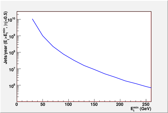
Figure 1.4: Number of jets with $E_{\scriptscriptstyle T}>{E_{\scriptscriptstyle T}}^{min}$ produced per year within $|\eta|<0.5$ (ALICE central barrel fiducial region) in minimum bias pp collisions at $\sqrt{s}$=14 TeV with luminosity $5\times 10^{30}$ cm^-2s^-1.

However, the rates estimated as above are production rates, which could only be exploited by fast dedicated hardware triggers. The EMCal will provide $\gamma$, $\pi^{0}$ and electrons triggers, that can be considered to be jet triggers of a sort, but the resulting sample will be dominated by relatively low-$E_{\scriptscriptstyle T}$ jets that fragment hard. A more refined selection of high-$E_{\scriptscriptstyle T}$ jets requires a jet trigger which sums energy over a finite area of phase space and finds the location of the patch with the highest integrated EMCal energy. The expected enhancement in statistics due to the EMCal trigger can be estimated by comparing the rates to tape of EMCal-triggered observables and equivalent observables using only charged tracks in the TPC and simple interaction (‘minimum bias’) triggers.

It has been estimated (see Sect. 6.8 in Ref. [2] and Sect. 7.1 in Ref. [6]) that the EMCal trigger will significantly increase the statistics, by a factor $\sim$ 70 for the $\pi^{0}$ trigger (relative to untriggered charged pion measurements), and by a factor $\sim$ 50 for finite-area jets of trigger patch-size $\Delta\eta\times\Delta\varphi=0.4\times 0.4$. The enhancement will be limited by the EMCal acceptance ($\sim 25$% of the TPC acceptance) and by its reduced effective value for jet triggers of finite extent in phase space relatively to small-area triggers ($\gamma$, $\pi^{0}$ and electrons). However, jet measurements incorporating both the EMCal and tracking have significantly better resolution and less bias than jet measurements based solely on charged particles. Thus, the EMCal-triggered jets provide more robust measurements even for modest trigger enhancements.

Depending on the setup of the Level-1 (L1) triggering detectors, the software High-Level-Trigger (HLT) will be used to either verify the L1 hypothesis or to solely inspect events at L2. A very simple online algorithm can run on the nodes of the HLT system to online search for jets using the full event information from the central tracking detectors. This algorithm is supposed to trigger if it finds at least one charged particle jet with more than $m$ GeV in a cone with $R$=0.7.

Trigger simulations [108] show that for $m$=30 GeV data rates in pp can be reduced by a factor of 100 relative to L1 rates, while keeping 1/5 of the events where ${E_{\scriptscriptstyle T}}^{min}>$ 50 GeV and slightly more than half of the events with ${E_{\scriptscriptstyle T}}^{min}>$ 100 GeV.

In case of a HLT running without the help of a jet trigger at L1 (as in the running scenario before the installation of the EMCal, and neglecting the possibility of a trigger provided by the TRD), the yields will drop by a factor of $\sim$ 350. The inspection rate of the HLT will be limited to the TPC maximum gating frequency of 1 kHz. The expected jet yield accumulated in one year for ${E_{\scriptscriptstyle T}}^{min}$= 100 GeV when ALICE is running in this configuration, is on the level of $10^{4}$ events, that is at the statistical limit for the analysis of jet fragmentation function at high-$z$.

Therefore a trigger with EMCal will be necessary to collect jet enriched data at $E_{\scriptscriptstyle T}>$ 100 GeV and extend the kinematic reach for inclusive jets to above $200$ GeV. For di-jets, with a trigger jet in the EMCal and the recoiling jet in the TPC acceptance, the kinematic reach will be about $170$ GeV.

1.11 Photons

The study of prompt photons processes, in which a real photon is created in the hard scattering of partons, offers possibilities for quantitative and clean tests of perturbative QCD (pQCD).

Lowest-order QCD predicts that prompt photons can be produced directly at a parton interaction vertex mainly by two processes: quark-antiquark annihilation ($\mathrm{q}+\bar{\mathrm{q}}\rightarrow\gamma+\mathrm{g}$) and quark-gluon Compton scattering ($\mathrm{g}+\mathrm{q}\rightarrow\gamma+\mathrm{q}$). Because of the latter process, which dominates the photon production in pp collisions, the measurement of prompt photons provides a sensitive means to extract information on the gluon momentum distribution inside the proton.

However, an additional source of high-$p_{\scriptscriptstyle T}$ prompt photons is due to the hard bremmstrahlung of final state partons (fragmentation photons). The latter is a long-distance process which is not perturbatively calculable, since it emerges from the collinear singularities occurring when a high-$p_{\scriptscriptstyle T}$ parton undergoes a cascade of successive splittings ending up with a photon. These singularities can be factorised and absorbed into a parton-to-photon fragmentation function which has to be determined experimentally and then included in the theoretical calculations.

The calculations of the production cross section of prompt photons at large $p_{\scriptscriptstyle T}$ have been carried out in the framework of perturbative QCD up to next-to-leading order (NLO) accuracy in $\alpha_{\scriptscriptstyle S}$. Their results have been found to describe rather well, within experimental errors and theoretical uncertainties, all the prompt photon data collected in pp and $\mathrm{p}$$\bar{\mathrm{p}}$ collisions over the last 25 years, both at fixed-target experiments ($\sqrt{s}$=20–40 GeV) and at colliders ($\sqrt{s}$=63–1800 GeV) [109, 110, 111].

Corrections for bremmstrahlung processes, for higher-order QCD diagrams and for higher-twist processes have been applied to the theory in recent years. Furthermore, full QCD calculations have been implemented up to NLO accuracy in more flexible Monte Carlo programmes at the partonic level, that allow to account easily for any kind of experimental cut [112, 113]. This is particularly important for the analyses of data collected in collider experiments, that require isolation criteria on photon candidates in order to suppress the huge background of secondary photons coming from hadron decays (mainly $\pi^{0}$, $\eta$) and to reduce the fragmentation component of prompt photon production.

It has been found that NLO pQCD predictions agree very well also with the most recent data collected by D0 [114] at the Tevatron Run II ($\sqrt{s}$=1.96 TeV) and by PHENIX [115] at the RHIC ($\sqrt{s}$=200 GeV). D0 has measured isolated prompt photons in the range $23<p_{\scriptscriptstyle T}<300$ GeV/c, whereas PHENIX has collected both inclusive and isolated photon data in the range $4<p_{\scriptscriptstyle T}<16$ GeV/c.

In a recent phenomenological analysis [116] all available prompt photon cross section data, including the most recent data from D0 and PHENIX, have been compared with NLO pQCD theoretical predictions evaluated at the common scale $\mu$=$p_{\scriptscriptstyle T}$/2. The data span two orders of magnitude in energy and there is an agreement over nine orders of magnitude in the cross sections between theory and experimental data.

An exception still comes from the fixed-target experiment E706 [117], at the Fermilab, that measured cross sections several times above theoretical predictions based on NLO pQCD calculations, with data and theory differing both in magnitude and shape. Although resummed calculations [118] accounting for recoil effects due to soft gluon radiation have reduced the theoretical uncertainties, E706 data still suggest large non perturbative parameters (i.e. an intrinsic $k_{T}$ [119]) not required by any other data sets. Data in the small-$x$ domain probed by LHC may contribute to clarify this issue, and its relation to the recoil resummation.

Predictions of production rates at LHC, obtained from calculations performed at next-to-leading order, still suffer from rather large uncertainties. These uncertainties are associated with the choice of renormalization, factorization and fragmentation scales [110, 120](of the order of 30%). As for the uncertainties associated to the structure functions they are expected to be relatively small (almost 10% in the lowest $p_{\scriptscriptstyle T}$ region).

However, for photon production at the LHC energies, a new kinematic region of small $x$ values ($x\approx x_{\mathrm{T}}=2p_{\scriptscriptstyle T}/\sqrt{s}$ will be explored, especially at low transverse momenta (for $p_{\scriptscriptstyle T}=2$ GeV/c, this corresponds to $x=3\times 10^{-4}$ at $\sqrt{s}=14$ TeV). Therefore one may question the reliability of straightforward NLO pQCD calculations in a kinematic domain where they have never been tested before, and where recoil corrections and resummed calculations may be required.

Furthermore, a specific feature of photon production at very high energy is related to the fact that the bremmstrahlung component becomes large and dominant at small $x$. The bremmstrahlung from a gluon is dominant at not too high $p_{\scriptscriptstyle T}$ (up to 20 GeV), whereas the production of photons from final-state quarks still remains important at higher $p_{\scriptscriptstyle T}$ (about 40% of the prompt photon yield at $p_{\scriptscriptstyle T}\sim$ 50 GeV/c [121]). However, the bremmstrahlung component is not well under control: in particular the gluon fragmentation function into a photon is not sufficiently constrained by previous data, and that results in a factor two uncertainty in the prompt photon rate for $p_{\scriptscriptstyle T}<20$ GeV. On the other hand the uncertainties in the quark fragmentation component might introduce difficulties in the calibration of the energy of a jet through the measurement of the energy of the recoiling photon in $\gamma$–jet events.

Figure 1.5 shows the predictions at the LHC energies of prompt and decay photon spectra [122]. Prompt photon spectra are calculated with NLO pQCD, while for decay photons the NLO pQCD estimates, extracted from calculated $\pi^{0}$ spectra, are compared to the predictions of PHOJET/DPMJET [123], an implementation of Dual Parton Model which includes soft physics (pomeron exchanges) and semi-hard dynamics.

The results show that the prompt photon spectrum is dominated by more than an order of magnitude by the decay photon spectrum, for which there is an excellent agreeement between the predictions of DPMJET and NLO pQCD.

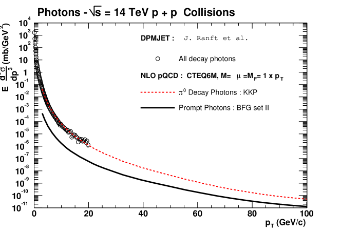
Figure 1.5: Comparison of prompt and decay photon spectra in pp collisions at $\sqrt{s}$=14 TeV.

NLO pQCD predictions for the ratio $\gamma_{prompt}/\pi^{0}$ are in the range $5\times 10^{-3}$–$10^{-2}$ for $p_{\scriptscriptstyle T}<10$ GeV/c, and in the range $10^{-2}$–$10^{-1}$ for $10<p_{\scriptscriptstyle T}<100$ GeV/c. The ratios, slowly increasing with $p_{\scriptscriptstyle T}$, are rather small at LHC energies, and isolation cuts will certainly be necessary to reduce the amount of the huge background due to decay photons.

At low $p_{\scriptscriptstyle T}$ the uncertainty in the photon spectrum is largely due to the choice of the gluon fragmentation function into photons, which is hardly constrained by the present data [124], and it goes from a factor up to 2.5 at 3 GeV/c to a factor 10% or less for $p_{\scriptscriptstyle T}>20$ GeV/c. The uncertainties associated to the structure functions are much smaller, of the order of 10% and 2.5% at low and high $p_{\scriptscriptstyle T}$, respectively.

Photons will be detected in ALICE by the Photon Spectrometer PHOS (see [125] and Sect. 3.9 in Ref. [1] for details), an electromagnetic calorimeter with high resolution but limited acceptance ($\eta<0.12$, $\Delta\Phi=120\mbox{${}^{\circ}$}$). The identification power of prompt photons in PHOS is limited by the background created by decay photons (mainly, $\pi^{0},\eta\rightarrow\gamma+\gamma$), and is optimal for photons with energy larger than 20 GeV. Below this value, decay and prompt photons cannot be efficiently distinguished on an event-by-event basis, and statistical methods are needed.

Photon measurements can be performed also with the EMCal, the second electromagnetic calorimeter in ALICE, which has coarser granularity compared to PHOS, but a factor eight larger phase space coverage, and so it may allow to extend ALICE photon measurements to higher $p_{\scriptscriptstyle T}$. However, the EMCal capabilities in the photon measurements will not be discussed here.

Two different procedures to select (with PHOS) prompt photons among inclusive photons are possible: Shower Shape Analysis (SSA), and Isolation Cut Method (ICM) (see [125] and Section 6.9 of Ref. [2]). The former identifies photons by analysing the shape of the shower in PHOS, and the latter tags and identifies a photon as prompt if it appears isolated, i.e., without charged particles emitted in the same direction.

To optimize the number of parameters conveying the maximal information about the shower topology, a principal component analysis was performed. The values of the two principal components, corresponding to the largest eigenvalues, have a Gaussian distribution. Low, medium and high purity photon samples can be defined by cutting at three, two and one standard deviations, respectively. For medium purity photon samples prompt photon identification efficiency is about 85% for pp collisions. The contamination from misidentified neutral pions ranges from 0% at $E_{\gamma}=40$ GeV to 40% at $E_{\gamma}=100$ GeV and the contamination from misidentified charged hadrons and neutrons ranges from 5% at $E_{\gamma}=20$ GeV to 15% at $E_{\gamma}=100$ GeV. Requiring higher purity photons the rejection improves at the cost of an important identification efficiency reduction. To improve the situation, additional identification procedures are required.

The main source of background to the prompt-photon spectrum at high $p_{\scriptscriptstyle T}$ is due to $\pi^{0}$ which at $p_{\scriptscriptstyle T}>40$ GeV/c produce single clusters in PHOS. Therefore isolation algorithms can be devised, that search for hadrons inside a cone centred around the direction ($\eta_{0},\>\varphi_{0}$) of high-$p_{\scriptscriptstyle T}$ photon candidates ($p_{\scriptscriptstyle T}>20$ GeV/c) identified by PHOS with the SSA method.

In the case of pp collisions a prompt photon identification probability of 100% and a $\pi^{0}$ misidentification probability of 3% were estimated from simulations with cone radius $R=0.2$.

Finally, our Monte Carlo simulations indicate that with PHOS the photon spectrum in pp (and also in Pb–Pb) collisions can be measured with the statistics of one standard year up to about 80–100 GeV/c, with a total systematic error of the order of 20%.

As already explained in another section of the present report, because of the large cross sections available for hard processes at LHC, exclusive jet measurements will be within reach. In particular, the measurement of jet topology (jet shape, jet heating, fragmentation functions, etc.) will require the identification of jets and the measurement of the parton (or jet) energy. A very attractive method of performing these studies is to tag jets with prompt photons emitted in the opposite direction to the jet direction.

A $\gamma$-tagging algorithm was developed [126] in ALICE to identify $\gamma$–jet events and to reconstruct the hadronic jet features. The algorithm was tuned for two experimental configurations of ALICE: (i) Charged particles are detected in the central tracking system and neutral particles in EMCal (this configuration is labelled as ‘TPC+EMCal’); (ii) Only the central tracking system is available and consequently only charged particles can be detected (this configuration is labeled as ‘TPC’).

The jet selection efficiency, defined as the ratio of the number of identified $\gamma$-tagged jets to the number of prompt photons found in PHOS was calculated using a Monte Carlo simulation. The efficiency for the configuration with EMCal is about 30%. For the configuration without EMCal we obtained an efficiency of 40–50%, because of: (i) the wider selection range, implying a lower identification quality; and (ii) the larger acceptance in azimuth of the central tracking system as compared to that of EMCal.

Jet fragmentation functions to be measured in a standard year of LHC running (for both pp and Pb–Pb collisions) were studied for identified $\gamma$–jet events in the $p_{\scriptscriptstyle T}$ range from 20 to 100 GeV/c. The fragmentation functions obtained for jet–jet events misidentified as $\gamma$–jet events were also studied. For pp collisions, we obtained a signal ($\gamma$–jet) to background (jet–jet) ratio of about 20 in the configuration without EMCal, and near to 100% background rejection for the setup with EMCal.

It is not advisable to use PHOS as a detector of jet neutral particles, because of its reduced acceptance. However, we may still consider another approach in which the prompt photon is detected in EMCal and jets are detected by the central tracking system. In such a setup, considering similar prompt photon identification features in PHOS and EMCal and the larger acceptance of the EMCal, the prompt photon detection would be enhanced by a factor 7 and consequently the statistical errors would be reduced by a factor 2.6. The EMCal granularity provides $\gamma/\pi^{0}$ discrimination via shower shape in the range $p_{\scriptscriptstyle T}\sim$ 10–30 GeV/c. Due to the low $\gamma/\pi^{0}$ ratio, however, a robust $\gamma$-jet measurement requires additional hadron rejection from isolation cuts. The $p_{\scriptscriptstyle T}$-reach up to $p_{\scriptscriptstyle T}\sim 30$ GeV/c matches well the statistical reach in a standard year for $\gamma$-jet analysis [6].

Therefore an experimental study of the fragmentation function of photon-tagged jets (i.e. the distribution of charged hadrons within jets as a function of the variable z, defined as $z=p_{\scriptscriptstyle T}/E_{\gamma}$) will be feasible with EMCal in one year up to $p_{\scriptscriptstyle T}\sim 30$ GeV/c.

Furthermore, in addition to single photon production and photon–jet (or photon–hadron) correlations, photon–photon correlations can be studied as well. The LO contributions to di-photon production are quark-antiquark annihilation ($\mathrm{q}+\bar{\mathrm{q}}\rightarrow\gamma+\gamma$) and gluon-gluon scattering ($\mathrm{g}+\mathrm{g}\rightarrow\gamma+\gamma$).

Processes where both photons originate from parton fragmentation or where one photon is prompt and the other photon comes from the fragmentation of a recoiling parton also contribute in LO. In this way, many of the inputs entering the theoretical calculations, in particular the fragmentation functions [127], can be tested.

However, di-photon final states are not only interesting to perform tests of pQCD but they are also signatures for many new physics processes, such as Higgs production at the LHC or large extra dimensions.

A further incentive to study prompt photons in pp collisions in ALICE comes from the need to provide a baseline against which medium effects observed in the measurements of prompt photons in heavy-ion collisions can be disentangled.

Medium effects in nucleus–nucleus collisions modify the vacuum production cross sections of prompt photons as measured in pp collisions: nuclear shadowing and in-medium parton energy loss lead to a suppression of the yield [128], whereas the intrinsic transverse momentum distribution of the partons [129, 130] and medium-induced photon radiation from quark jets [131] enhance the yield.

On the other hand an expected signature of Quark Gluon Plasma formation in central heavy-ion collisions is an increased production of thermal photons, emitted in radiation processes, roughly in the $p_{\scriptscriptstyle T}$ range $1<p_{\scriptscriptstyle T}<10$ GeV/c; therefore it is important to understand non-thermal production mechanisms in pp collisions in the same energy range.

Furthermore, in the case of Pb–Pb collisions, photons emerge almost unaltered from the dense strongly-interacting medium and provide a measurement of the original energy and direction of the parton emitted in the opposite direction. Therefore medium effects will be also identified through modifications of the jet fragmentation function, i.e. by the redistribution of the jet energy rather than by reduction of jet rate. A broadening of the distribution of the jet-particle momenta perpendicular to jet axis ($j_{T}$), directly related to the colour density of the medium, is also expected [132].

1.12 Exotica: mini black holes from large extra dimensions

The concept of large extra dimensions provides a way of solving the hierarchy problem which concerns the weakness of gravity compared with strong and electro-weak forces. The extra space-dimensions, beyond the usual three dimensions, are assumed to be compactified. i.e. finite, so they are too small to be normally detected. A consequence of large extra dimensions is that mini black holes (BH) could exist at the greatly reduced Planck mass of around 1 TeV, and thus might be produced at the LHC in pp collisions.

Quantitative calculations for BH production and detection in the ALICE experiment at the LHC have been presented in Ref. [133, 134]. In this study the BH event generator code CHARYBDIS [135] has been used, that is coupled to PYTHIA code for parton evolution and hadronization. Taking advantage of the large-acceptance and high-precision tracking detectors available in ALICE, namely the Inner Tracking System (ITS), the Time Projection Chamber (TPC) and the Transition Radiation Detector (TRD), two event-by-event hadronic observables were used for BH studies: charged particle multiplicity and summed-$p_{\scriptscriptstyle T}$.

The conclusions drawn from this study are that under the standard running conditions, with a minimum-bias trigger running for four months at the LHC initial luminosity, and with a maximum data acquisition rate in ALICE of 100 Hz, only a few BH events could be visible above the QCD background and only for a Planck mass $M_{P}=1$  TeV, occurring for multiplicity above 200 and summed-$p_{\scriptscriptstyle T}$ above 0.5 TeV/c.

However it is possible to improve this situation, when applying a simple charged particle multiplicity trigger to ALICE events, which is expected to greatly reduce the QCD background allowing for significant BH signals to be detected.

For charged multiplicity, the sensitivity to $M_{P}$ is raised to 2 TeV and hundreds of BH events above background corresponding to this case are expected for multiplicity greater than 250. An even better situation occurs for summed $p_{\scriptscriptstyle T}$ distribution, since ten of thousands of BH events above background are expected for the $M_{P}=1$  TeV case, and tens of BH events even for the $M_{P}=5$  TeV case.

The signature for BH creation from these simple distributions is seen to be an abrupt flattening of their slope, as the transition from QCD to BH-dominated charged particle production takes place.

1.13 Concluding remarks

We have presented in this document the potentialities of the ALICE detector in the field of pp physics. A special emphasis has been given to the minimum-bias pp physics programme, that is expected to dominate the start-up of the LHC operation. The importance of such a programme has been pointed out both for its intrinsic interest and also as a reference system for comparison with the nucleus–nucleus and proton–nucleus studies in ALICE. However, it has been shown that significant contributions can be given by ALICE also in other pp physics topics.

The complete ALICE detector has significant advantages compared to other LHC detectors in pp physics attainable at the low luminosity stage of the LHC, mainly because of its low momentum thereshold, good momentum resolution and unique capacity to measure and identify a large spectrum of particles, including baryons and strange particles. On the other hand the ALICE momentum and angular resolution is at least comparable to the one of the other LHC experiments up to 10 GeV/c. Moreover ALICE has the capability to measure the transverse momentum of charged particles in the range $|\eta|\leq 1.5$ and, by exploiting both the Silicon Pixel Detector and the Forward Multiplicity Detector, charged track multiplicity in the range $-3.4\leq\eta\leq 5.1$. Therefore in many essential ways the ALICE pp programme described here is complementary to those possible with other LHC experiments. And especially at the early stage of the LHC operation, ALICE will be able to provide a significant contribution to this field.

1.14 Acknowledgements

The author of the present contribution expresses his thanks to Andreas Morsch, Panos Christakoglou, Rainer Schicker, Jan Fiete Grosse-Oetringhaus, Alberto Giovannini and Roberto Ugoccioni for useful help and suggestions, and he gratefully acknowledges Nestor Armesto for having provided his NLO calculations of jet rates at the LHC.

Measurement of heavy-flavour production with ALICE

A. Dainese for the ALICE Collaboration.

2.15 Introduction

The ALICE experiment [1] will study nucleus–nucleus collisions at the LHC, with a centre-of-mass energy per nucleon–nucleon collision $\sqrt{s_{\scriptscriptstyle{{\rm NN}}}}=5.5~{}\mathrm{TeV}$ for the Pb–Pb system, in order to investigate the properties of QCD matter at energy densities of up to several hundred times the density of atomic nuclei. Under these conditions a deconfined state of quarks and gluons is expected to be formed.

The measurement of open charm and open beauty production allows to investigate the mechanisms of heavy-quark production, propagation and hadronization in the hot and dense medium formed in high-energy nucleus–nucleus collisions. Of particular interest is the study of the effects of parton energy loss on c and b quarks. Believed to be at the origin of the jet quenching phenomena observed in Au–Au collisions at the Relativistic Heavy Ion Collider (RHIC), energy loss is expected to depend on the properties of the medium (gluon density and volume) and on the properties of the ‘probe’ (colour charge and mass). The open charm and open beauty cross sections are also needed as a reference to measure the effect of the transition to a deconfined phase on the production of quarkonia. Heavy-quark production measurements in proton–proton and proton–nucleus collisions at the LHC, besides providing the necessary baseline for the study of medium effects in nucleus–nucleus collisions, are interesting per se, as a test of QCD in a new energy domain.

2.16 Heavy-flavour production from pp to Pb–Pb

Heavy-quark pairs ($\rm Q\overline{Q}$) are expected to be produced in primary partonic scatterings with large virtuality $Q^{2}>(2m_{\rm Q})^{2}$ and, thus, on small temporal and spatial scales, $\Delta t\sim\Delta r\sim 1/Q\,{\buildrel<\over{{}_{\sim}}}\,0.1~{}\mathrm{fm}$ for $m_{\rm c}=1.2~{}\mathrm{GeV}$. In nucleus–nucleus reactions, this implies that the initial production process is not affected by the presence of the dense medium formed in the collision. Given the large virtualities, the baseline production cross sections in nucleon–nucleon collisions can be calculated in the framework of perturbative QCD (pQCD). For the estimate of baseline production yields in nuclear collisions (to be used for performance studies and preparation of the analysis strategies), scaling of the yields with the average number $\left\langle N_{\rm coll}\right\rangle$ of inelastic nucleon–nucleon collisions (binary scaling) is usually assumed:

$${\rm d}^{2}N^{\scriptstyle\rm Q}_{\rm AA(pA)}/{\rm d}p_{\rm t}{\rm d}y=\left\langle N_{\rm coll}\right\rangle\times{\rm d}^{2}N^{\scriptstyle\rm Q}_{\rm pp}/{\rm d}p_{\rm t}{\rm d}y\,.$$ (2.1)

The expected $\mathrm{c\overline{c}}$ and $\mathrm{b\overline{b}}$ production yields for different collision systems at the LHC are reported in the first line of Table 2.1 [2]. These numbers, assumed as the baseline for ALICE simulation studies, are obtained from pQCD calculations at NLO [3], including the nuclear modification of the parton distribution functions (PDFs) [4] in the Pb nucleus (details on the choice of pQCD parameter values and PDF sets can be found in [2]). Note that the predicted yields have large uncertainties, of about a factor 2, estimated by varying the values of the calculation parameters. An illustration of the theoretical uncertainty bands for the D and B meson cross sections will be shown in section 2.17, along with the expected sensitivity of the ALICE experiment.

Table 2.1: Expected $\rm Q\overline{Q}$ yields per event at the LHC, from NLO pQCD calculations [2]. For p–Pb and Pb–Pb, Modification of the PDFs in nuclei is taken into account and $N_{\rm coll}$ scaling is assumed.

colliding system	pp	p–Pb	Pb–Pb
$\sqrt{s_{\scriptscriptstyle{{\rm NN}}}}$	14 TeV	8.8 TeV	5.5 TeV
centrality	–	min. bias	0–5% $\sigma^{\rm inel}$
$\mathrm{c\overline{c}}$ pairs	0.16	0.78	115
$\mathrm{b\overline{b}}$ pairs	0.0072	0.029	4.6

2.17 Heavy-flavour detection in ALICE

The ALICE experimental setup, described in detail in [1, 5], was designed in order to allow the detection of ${\rm D}$ and ${\rm B}$ mesons in the high-multiplicity environment of central Pb–Pb collisions at LHC energy, where a few thousand charged particles might be produced per unit of rapidity. The heavy-flavour capability of the ALICE detector is provided by:

• Tracking system; the Inner Tracking System (ITS), the Time Projection Chamber (TPC) and the Transition Radiation Detector (TRD), embedded in a magnetic field of $0.5$ T, allow track reconstruction in the pseudorapidity range $-0.9<\eta<0.9$ with a momentum resolution better than 2% for $p_{\rm t}<20~{}\mathrm{GeV}/c$ and a transverse impact parameter resolution better than $60~{}\mathrm{\mu m}$ for $p_{\rm t}>1~{}\mathrm{GeV}/c$ (the two innermost layers of the ITS are equipped with silicon pixel detectors).

• Particle identification system; charged hadrons are separated via ${\rm d}E/{\rm d}x$ in the TPC and in the ITS and via time-of-flight measurement in the Time Of Flight (TOF) detector; electrons are separated from charged hadrons in the dedicated Transition Radiation Detector (TRD), and in the TPC; muons are identified in the muon spectrometer covering the pseudo-rapidity range $-4<\eta<-2.5$ [6].

Detailed analyses [7], based on full simulation of the detector and of the background sources, have shown that ALICE has a good potential to carry out a rich heavy-flavour Physics programme. In section 2.18 we describe the expected performance for the exclusive reconstruction of ${\rm D^{0}\to K^{-}\pi^{+}}$ decays in pp, p–Pb and Pb–Pb collisions, and the estimated sensitivity for the comparison with pQCD predictions, for the pp case. In section 2.19 we present the perspectives for the measurement of beauty production in the semi-electronic channel in pp collisions. The expected performance for beauty production measurement using muons is described in section 2.20.

For all studies a multiplicity of ${\rm d}N_{\rm ch}/{\rm d}y=6000$ was assumed for central Pb–Pb collisions. We report the results corresponding to the expected statistics collected by ALICE per LHC year: $10^{7}$ central (0–5% $\sigma^{\rm inel}$) Pb–Pb events at luminosity $\mathcal{L}_{\rm Pb-Pb}=5\times 10^{26}~{}\mathrm{cm}^{-2}{\rm s}^{-1}$ and $10^{9}$ pp events at $\mathcal{L}_{\rm pp}^{\rm ALICE}=5\times 10^{30}~{}\mathrm{cm}^{-2}{\rm s}^{-1}$, in the barrel detectors; the muon spectrometer will collect about 40 times larger samples (i.e.  $4\times 10^{8}$ central Pb–Pb events).

2.18 Measurement of charm production in the $\mbox{$\mathrm{D^{0}}$}\to K^{-}\pi^{+}$ channel

One of the most promising channels for open charm detection is the ${\rm D^{0}\to K^{-}\pi^{+}}$ decay (and its charge conjugate) which has a branching ratio (BR) of about $3.8\%$. The expected production yields (${\rm BR}\times{\rm d}N/{\rm d}y$ at $y=0$) for ${\rm D^{0}}$ (and ${\rm\overline{D^{0}}}$) mesons decaying in a ${\rm K^{\mp}\pi^{\pm}}$ pair in central Pb–Pb (0–$5\%~{}\sigma^{\rm inel}$) at $\sqrt{s_{\scriptscriptstyle{{\rm NN}}}}=5.5~{}{\rm TeV}$, in minimum-bias p–Pb collisions at $\sqrt{s_{\scriptscriptstyle{{\rm NN}}}}=8.8~{}{\rm TeV}$ and in pp collisions at $\sqrt{s}=14~{}{\rm TeV}$ are, in the order, $5.3\times 10^{-1}$, $3.7\times 10^{-3}$ and $7.5\times 10^{-4}$ per event.

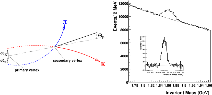
Figure 2.6: Schematic representation of the ${\rm D^{0}\to K^{-}\pi^{+}}$ decay (left). ${\rm K\pi}$ invariant-mass distribution corresponding to $10^{7}$ central Pb–Pb events (right); the background-subtracted distribution is shown in the insert.

Figure 2.6 (left) shows a sketch of the decay: the main feature of this topology is the presence of two tracks with impact parameters $d_{0}\sim 100~{}\mathrm{\mu m}$. The detection strategy to cope with the large combinatorial background from the underlying event is based on:

1. selection of displaced-vertex topologies, i.e. two tracks with large impact parameters and small pointing angle $\Theta_{\rm p}$ between the ${\rm D^{0}}$ momentum and flight-line (see sketch in Fig. 2.6);

2. identification of the K track in the TOF detector;

3. invariant-mass analysis (see $p_{\rm t}$-integrated distribution in Pb–Pb after selections in Fig. 2.6).

This strategy was optimized separately for pp, p–Pb and Pb–Pb collisions, as a function of the ${\rm D^{0}}$ transverse momentum [7].

Figure 2.7 shows the expected relative statistical errors on the measured ${\rm D^{0}}$ $p_{\rm t}$ distribution for pp collisions at 14 TeV ($10^{9}$ events, i.e. 7 months at nominal pp luminosity for ALICE) and central Pb–Pb collisions at 5.5 TeV ($10^{7}$ events, i.e. 1 month at nominal Pb–Pb luminosity). The accessible $p_{\rm t}$ range is $1$–$20~{}\mathrm{GeV}/c$ for Pb–Pb and $0.5$–$20~{}\mathrm{GeV}/c$ for pp (and p–Pb, not shown), with a point-by-point statistical error better than 15–20%. The statistical error on the cross section for $p_{\rm t}>p_{\rm t}^{\rm min}$ is estimated to be of about 3% in pp and p–Pb ($p_{\rm t}^{\rm min}=0.5~{}\mathrm{GeV}/c$) and of about 7% in central Pb–Pb ($p_{\rm t}^{\rm min}=1~{}\mathrm{GeV}/c$). The systematic error (acceptance and efficiency corrections, centrality selection for Pb–Pb) is expected to be smaller than 20%. More details are given in [7].

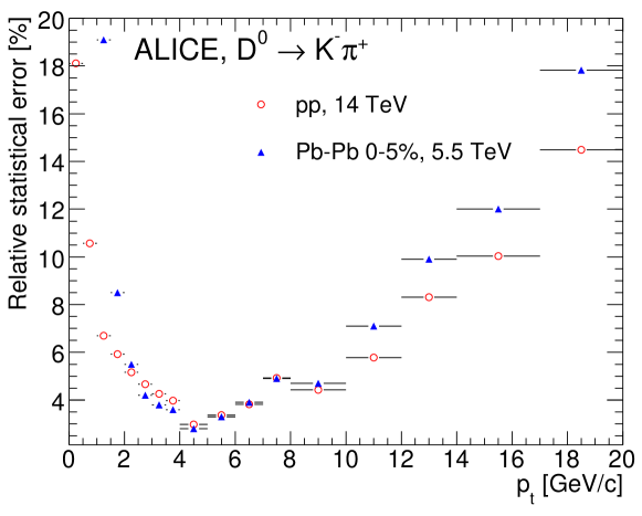
Figure 2.7: Expected relative statistical errors for the measurement in ALICE of the production cross section of $D^{0}$ mesons in 0–5% central Pb–Pb and in pp collisions.

For the case of pp collisions, the experimental errors on the $p_{\rm t}$-differential cross section are expected to be significantly smaller than the current theoretical uncertainty from perturbative QCD calculations. In Fig. 2.8 we superimpose the simulated ALICE measurement points to the prediction bands from the MNR fixed-order massive calculation [3] and from the FONLL fixed-order next-to-leading log calculation [8, 9]. The perturbative uncertainty bands were estimated by varying the values of the charm quark mass and of the factorization and renormalization scales. The comparison shows that ALICE will be able to perform a sensitive test of the pQCD predictions for charm production at LHC energy.

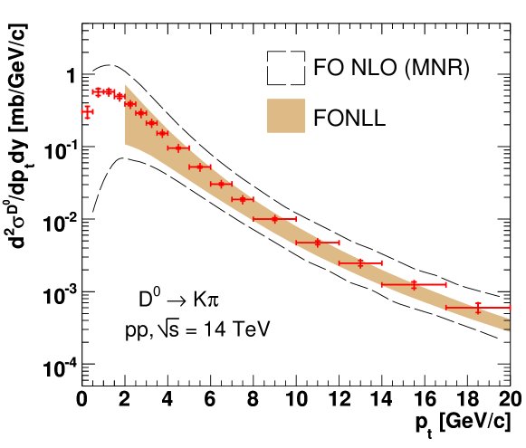
Figure 2.8: Sensitivity on d${}^{2}\sigma^{\rm D^{0}}/$d$p_{\rm t}$d$y$, in pp at 14 TeV, compared to NLO pQCD predictions from the MNR [3] and FONLL [8] calculations. The inner error bars represent the statistical errors, the outer error bars represent the quadratic sum of statistical and $p_{\rm t}$-dependent systematic errors. A normalization error of 5% is not shown.

2.19 Measurement of beauty production in the semi-electronic decay channel

The production of open beauty can be studied by detecting the semi-electronic decays of beauty hadrons, mostly B mesons. Such decays have a branching ratio of $\simeq 10\%$ (plus 10% from cascade decays ${\rm b\to c}\to e$, that only populate the low-$p_{\rm t}$ region in the electron spectrum). The expected yields (${\rm BR}\times{\rm d}N/{\rm d}y$ at $y=0$) for ${\rm b}\to e+X$ plus ${\rm b}\to{\rm c}\,(\to e+X)+X^{\prime}$ in central Pb–Pb($0$–$5\%~{}\sigma^{\rm inel}$) at $\sqrt{s_{\scriptscriptstyle{{\rm NN}}}}=5.5~{}{\rm TeV}$ and in in pp collisions at $\sqrt{s}=14~{}{\rm TeV}$ are $1.8\times 10^{-1}$ and $2.8\times 10^{-4}$ per event, respectively.

The main sources of background for the signal of beauty-decay electrons are: decays of primary D mesons, which have a branching ratio of $\approx 10\%$ in the semi-electronic channels, and an expected production yield about 20 times larger than B mesons (see Table 2.1); decays of light mesons (mainly $\rho$, $\omega$, K) and neutral pion Dalitz decays ($\pi^{0}\to\gamma e^{+}e^{-}$); conversions of photons in the beam pipe or in the inner layers of the ITS; charged pions misidentified as electrons. Given that electrons from beauty have an average impact parameter $d_{0}\simeq 500~{}\mathrm{\mu m}$ and a hard momentum spectrum, it is possible to obtain a high-purity sample with a strategy that relies on:

1. Electron identification with a combined ${\rm d}E/{\rm d}x$ (TPC) and transition radiation selection, which is expected to reduce the pion contamination by a factor of about $10^{4}$ at low $p_{\rm t}$.

2. Impact parameter ($d_{0}$) cut to reject misidentified $\pi^{\pm}$ and $e^{\pm}$ from Dalitz decays and $\gamma$ conversions (the latter have small impact parameter for $p_{\rm t}\,{\buildrel>\over{{}_{\sim}}}\,1~{}\mathrm{GeV}/c$) and to reduce the contribution of electrons from charm decays. We have optimized the value of the impact parameter cut as a function of the transverse momentum in order to minimize the total errors (statistical + systematic). The typical value of the cut is $d_{0}>200~{}\mu m$.

The residual contamination of about 10%, mainly accumulated in the low-$p_{\rm t}$ region, of electrons from prompt charm decays, from misidentified charged pions and $\gamma$-conversion electrons can be evaluated and subtracted using a Monte Carlo simulation tuned to reproduce the measured cross sections for pions and $\rm D^{0}$ mesons. Figure 2.9 shows the expected relative statistical errors for pp collisions at 14 TeV ($10^{9}$ events, i.e. 7 months at nominal LHC luminosity) and central Pb–Pb collisions at 5.5 TeV ($10^{7}$ events, i.e. 1 month at nominal LHC luminosity).

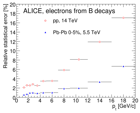
Figure 2.9: Expected relative statistical errors for the measurement in ALICE of the production cross section of B-decay electrons in 0–5% central Pb–Pb and in pp collisions.

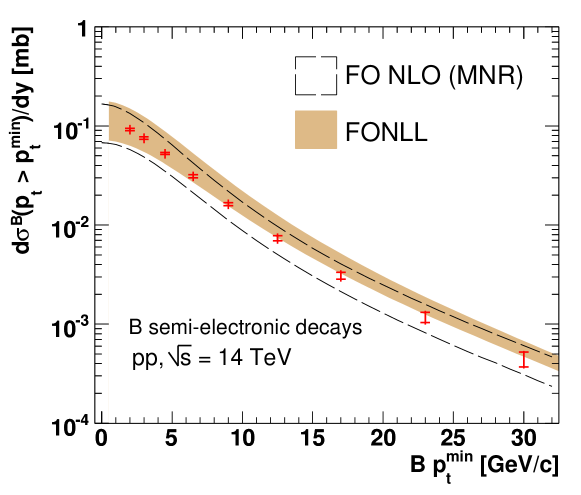
Figure 2.10: Sensitivity on d$\sigma^{\rm B}(p_{\rm t}>p_{\rm t}^{\rm min})/$d$y$, in pp at 14 TeV, compared to NLO pQCD predictions from the MNR [3] and FONLL [8] calculations. Error bars are defined as in Fig. 2.8.

We tested the possibility to infer the $p_{\rm t}^{\rm min}$-differential cross section for beauty mesons, ${\rm d}\sigma^{B}(p_{\rm t}>p_{\rm t}^{min})/{\rm d}y$, from the electron-level cross section using a procedure similar to that developed by the UA1 Collaboration [10]. The method, described in detail in Ref. [7], is based on Monte Carlo simulation and it relies on the fact that the B meson decay kinematics, measured and studied in several experiments, is well understood. It has been shown [7] for the Pb–Pb case that, if electrons with $p_{\rm t}>2~{}\mathrm{GeV}/c$ are used (below this limit, the correlation between the electron and B meson momenta is very poor), the additional systematic error is negligible with respect to the systematic uncertainties already present at the electron level.

Figure 2.10 presents the expected ALICE performance for the measurement of the $p_{\rm t}^{min}$-differential cross section of B mesons, ${\rm d}\sigma^{B}(p_{\rm t}>p_{\rm t}^{min})/{\rm d}y$ vs. $p_{\rm t}^{min}$ averaged in the range $|y|<1$. For illustration of the sensitivity in the comparison to pQCD calculations, we report in the same figure the predictions and the theoretical uncertainty bands from the perturbative calculations in the MNR [3] and FONLL [8, 9] approaches. It can be seen that the expected ALICE performance for $10^{9}$ events will provide a meaningful comparison with pQCD predictions.

2.20 Measurement of beauty production in the semi-muonic decay channel

Beauty production can be measured also in the ALICE muon spectrometer, $-4<\eta<-2.5$, analyzing the single-muon $p_{\rm t}$ distribution and the opposite-sign di-muons invariant mass distribution [7].

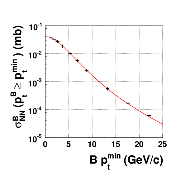
Figure 2.11: Minimum-$p_{\rm t}$-differential production cross section per nucleon–nucleon collision for B mesons with $-4<y<-2.5$ in central Pb–Pb collisions, as expected to be measured from the single-muon data set. Statistical errors (represented by the thickness of the horizontal bars) corresponding to $4\times 10^{8}$ events and $p_{\rm t}$-dependent systematic errors (vertical bars) are shown. A normalization error of 10% is not shown. The line indicates the input cross section.

The main backgrounds to the ‘beauty muon’ signal are $\pi^{\pm}$, $\rm K^{\pm}$ and charm decays. The cut $p_{\rm t}>1.5~{}\mathrm{GeV}/c$ is applied to all reconstructed muons in order to increase the signal-to-background ratio. For the opposite-sign di-muons, the residual combinatorial background is subtracted using the technique of event-mixing and the resulting distribution is subdivided into two samples: the low-mass region, $M_{\mu^{+}\mu^{-}}<5~{}\mathrm{GeV}$, dominated by di-muons originating from a single b quark decay through $\rm b\to c(\to\mu^{+})\mu^{-}$ ($\rm BD_{\rm same}$), and the high-mass region, $5<M_{\mu^{+}\mu^{-}}<20~{}\mathrm{GeV}$, dominated by $\mbox{$\mathrm{b\overline{b}}$}\to\mu^{-}\mu^{+}$, with each muon coming from a different quark in the pair ($\rm BB_{\rm diff}$). Both samples have a background from $\mbox{$\mathrm{c\overline{c}}$}\to\mu^{+}\mu^{-}$ and a fit is performed to extract the charm- and beauty-component yields. The single-muon $p_{\rm t}$ distribution has three components with different slopes: K and $\pi$, charm, and beauty decays. The first component is subtracted on the basis of the identified hadron spectra measured in the central barrel. Then, a fit technique allows to extract a $p_{\rm t}$ distribution of muons from beauty decays. A Monte Carlo procedure, similar to that used for semi-electronic decays, allows to extract B-level cross sections for the data sets (low-mass $\mu^{+}\mu^{-}$, high-mass $\mu^{+}\mu^{-}$, and $p_{\rm t}$-binned single-muon distribution), each set covering a different B-meson $p_{\rm t}>p_{\rm t}^{\rm min}$ region. The results for central Pb–Pb collisions at $\sqrt{s_{\scriptscriptstyle{{\rm NN}}}}=5.5~{}\mathrm{TeV}$ using only the single muons are shown in Fig. 2.11. Since only minimal cuts are applied, the reported statistical errors (represented by the thickness of the horizontal bars) are very small and the high-$p_{\rm t}$ reach is excellent. Similar performance, in terms of $p_{\rm t}$ coverage, is expected for pp collisions at $\sqrt{s}=14~{}\mathrm{TeV}$. The main sources of systematic errors (vertical bars) are: corrections for acceptance and efficiency, subtraction of the background muons from charged pion and kaon decays, and fit procedure to separate the beauty and charm components.

2.21 Conclusions

We presented the performance of ALICE for the measurement of charm and beauty production in proton–proton collisions at $\sqrt{s}=14~{}\mathrm{TeV}$ and central Pb–Pb collisions at $\sqrt{s_{\scriptscriptstyle{{\rm NN}}}}=5.5~{}\mathrm{TeV}$. For the pp case, these measurements will provide sensitive tests for perturbative QCD in a new energy domain. They will also be essential for a comparison with the corresponding measurements in Pb–Pb collisions, for example for the investigation of c and b quark in-medium energy loss [11].

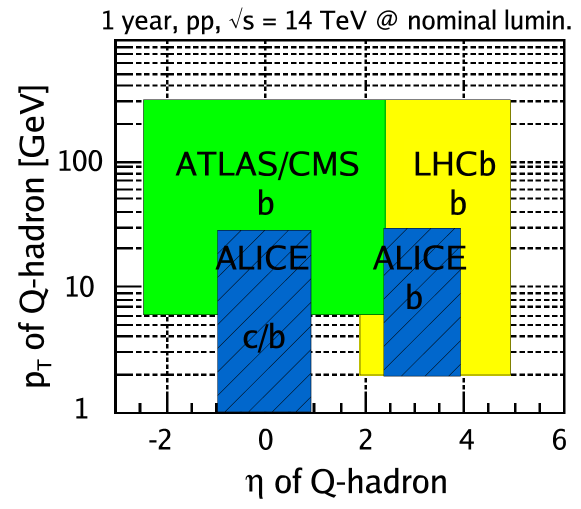
Figure 2.12: Schematic acceptances in transverse momentum and pseudorapidity for open heavy flavour hadrons (indicated as “Q-hadrons”) in the four LHC experiments [12]. The high-$p_{\rm t}$ coverages correspond to one year (i.e. 7 months) of running at nominal luminosity (see text). [Note that the acceptance of the ALICE muon spectrometer, indicated as $-4<\eta<-2.5$ in the ALICE coordinate system, is reported in the figure as $2.5<\eta<4$ to display the overlap with the acceptance of LHCb.]

We conclude by comparing, for pp collisions at $\sqrt{s}=14~{}\mathrm{TeV}$, the ALICE envisaged acceptance for heavy-flavour production measurements to that of the other LHC experiments. Figure 2.12 (from the proceedings of the workshop “HERA and the LHC” [12]) shows schematically the $p_{\rm t}$ vs. $\eta$ acceptances for charm (c) and beauty (b) hadrons in the four experiments, as expected for one year of running at nominal luminosity (note that the value of the luminosity is different for each experiment: $\mathrm{10^{34}~{}cm^{-2}s^{-1}}$ for ATLAS and CMS, $(2$–$5)\times\mathrm{10^{32}~{}cm^{-2}s^{-1}}$ for LHCb, and $\mathrm{5\times 10^{30}~{}cm^{-2}s^{-1}}$ for ALICE). ATLAS and CMS have similar acceptances for beauty measurements; the minimum accessible $p_{\rm t}$ is larger than for ALICE because of the strong magnetic fields, which in turn, together with the high luminosity, allow to cover transverse momenta up to 200–300 $\mathrm{GeV}/c$, and because of the larger material budget (amount of material) in the inner tracking detectors. In terms of acceptance for beauty measurements, ALICE overlaps with ATLAS and CMS at central rapidity and with LHCb at forward rapidity. The moderate magnetic field allows measurements down to transverse momenta of about $2~{}\mathrm{GeV}/c$ for B mesons in the muon arm and in the barrel, and down to less than $1~{}\mathrm{GeV}/c$ for D mesons in the barrel.

Quarkonia detection with the ALICE Muon Spectrometer in pp collisions at 14 TeV and PDF sensitivity in the low x region

D. Stocco for the ALICE Collaboration

The ALICE Muon Spectrometer [1] is a forward detector, with acceptance in the polar angle interval $171^{\circ}<\theta<178^{\circ}$. It consists of a composite absorber ($\sim 10\lambda_{int}$), made with layers of both high and low Z materials, starting 90 cm from the interaction vertex, a large dipole magnet with a 0.7 T magnetic field and 10 planes of high-granularity tracking stations. A second absorber ($\sim 7\lambda_{int}$ of iron) at the end of the spectrometer and four more detector planes are used for muon identification and triggering. The spectrometer is shielded throughout its length by a dense absorber tube surrounding the beam pipe. The spectrometer was designed in order to detect quarkonia down to $p_{\mathrm{t}}\sim 0$ in the rapidity region $-4.0<y<-2.5$.

The study of quarkonia production in pp collisions presents a twofold interest. On the one hand, pp measurements represent a baseline for quarkonia production in heavy-ion collisions. On the other, they have an intrinsic interest since they are expected to shed light on quarkonia production mechanisms by testing the existing theoretical models in an unexplored energy regime. In this respect, the relevant observables are quarkonia cross sections and $p_{\mathrm{t}}$ distributions. In addition, the rapidity acceptance of the Muon Spectrometer for quarkonia will allow access to PDFs at very small $x$.

The results of simulation studies of the ALICE Muon Spectrometer physics performance for quarkonia detection in proton-proton collisions at $\sqrt{s}=14$ ${\rm TeV}$ are presented.

The simulation input is provided by the Color Evaporation Model (CEM) [2, 3] predictions. In this model the quarkonium production cross section is a measurable fraction ($F_{C}$) of all $Q\bar{Q}$ pairs below the $H\bar{H}$ threshold (where $H$ is the lowest mass heavy flavor hadron) without any constraints on the color or spin of the final state. The $Q\bar{Q}$ pair then neutralizes its color by interaction with the collision-induced color field. At leading order, the production cross section of quarkonium state $C$ in an $AB$ collision is:

$$\sigma_{C}^{\scriptscriptstyle{CEM}}=F_{C}\sum_{i,j}{\int_{4m_{Q}^{2}}^{4m_{H}^{2}}{\mathrm{d}\hat{s}\int{\mathrm{d}x_{1}\mathrm{d}x_{2}\,f_{i/A}(x_{1},\mu^{2})f_{j/B}(x_{2},\mu^{2})\hat{\sigma}_{ij}(\hat{s})\delta(\hat{s}-x_{1}x_{2}s)}}}$$ (3.2)

where $A$ and $B$ can be any hadron or nucleus, $ij=$$q\bar{q}$ or $gg$, $\hat{\sigma}_{ij}(\hat{s})$ is the $ij\rightarrow$ $Q\bar{Q}$ subprocess cross section and $f_{i/A}(x_{1},\mu^{2})$ is the parton density in the hadron or nucleus. Finally, $s$ and $\hat{s}$ are respectively the hadronic and partonic center of mass energies. The results presented here have been obtained with the set of parameters (from [3]) listed in Table 3.2.

The resulting cross sections in pp collisions, which will be referred to as prompt (and include direct production and feed-down from higher mass resonances within the same family), are shown in the same table. The values take into account branching ratios in the $\mu^{+}\mu^{-}$ channel as well.

	J/$\psi$	$\psi^{\prime}$	$\Upsilon$	$\Upsilon^{\prime}$	$\Upsilon^{\prime\prime}$
$\sigma$ ($\mu$b)	3.18	0.057	0.028	0.0069	0.0041
$F_{C}$	0.0144	0.0021	0.0201	0.00636	0.00335
PDF	MRST98 NLO		MRST98 NLO
$m_{q}$	1.2		4.5
$\mu/m_{q}$	2		2

Table 3.2: CEM parameters and resulting cross sections for quarkonia production in pp collisions at 14 ${\rm TeV}$. Cross sections include feed-down from higher mass resonances and branching ratios in muon pairs. The adopted PDF comes from calculations at NLO precision by Martin-Roberts-Stirling-Thorne in 1998 (see [4]).

In addition to prompt J/$\psi$ and $\psi^{\prime}$, also those from B decay are taken into account in this study. These cross sections have been obtained from the open beauty cross section using the $B\rightarrow\mbox{J\kern-0.50003pt/\kern-0.50003pt$\psi$}+X$ and $B\rightarrow\mbox{$\psi^{\prime}$}+X$ branching ratios.

The rapidity distributions for prompt production of the different quarkonia states are a parameterization of CEM predictions, while the $p_{\mathrm{t}}$ distributions are obtained by extrapolating to LHC energies those measured by the CDF experiment at $\sqrt{s}\sim 2$ ${\rm TeV}$ [5, 6].

The invariant mass continuum from semileptonic decay of beauty and charm hadrons and from weak decay of pions and kaons was produced with PYTHIA. $\mathrm{c\overline{c}}$ and $\mathrm{b\overline{b}}$ pairs were produced with a cross section of 11.2 and 0.51 mb, respectively [7, 8].

The so obtained $\mathrm{b\overline{b}}$ pairs were then used in order to get the J/$\psi$ and $\psi^{\prime}$ from B decay. Since the Muon Spectrometer will not be able to distinguish in a direct way between the two main sources of charmonia (prompt and coming from B decay), both contributions were summed together to evaluate the expected yields.

Since the full simulation of a sufficient number of events would require long computing times, a fast simulation was performed. Such a method is based on the parameterization of the whole spectrometer response at the single muon level. Given a muon of momentum $p$ generated at the interaction point with polar and azimuthal angles $\theta$ and $\varphi$, the fast simulation applies the smearing of the apparatus and gives the reconstructed $p^{\prime}$, $\theta^{\prime}$ and $\varphi^{\prime}$ together with the detection probability for that muon.

At the trigger level, loose cuts on single muon $p_{\mathrm{t}}$ are applied: a low cut for muons from charmonia resonances and a high cut for muons from bottomonia ones. Such trigger cuts are not sharp but they roughly correspond to $p_{\mathrm{t}}$ $\sim$ 1 GeV$\kern-1.49994pt/\kern-1.19995ptc$ and $p_{\mathrm{t}}$ $\sim$ 2 GeV$\kern-1.49994pt/\kern-1.19995ptc$, respectively.

The simulations allow to calculate the global geometrical acceptances for quarkonia, integrated over the whole phase space, which are found to be of the order of 4% for both J/$\psi$ and $\Upsilon$. The detection probabilities for the different onium states were computed by applying the trigger and tracking response to each muon of the pair. The rapidity (transverse momentum) dependencies of the detection probabilities for J/$\psi$ and $\Upsilon$ are shown in the right (left) panels of Fig. 3.13. These were computed as the ratio between the number of detected and generated quarkonia at given $y$ ($p_{\mathrm{t}}$). The depletion in the $p_{\mathrm{t}}$ detection probabilities at low $p_{\mathrm{t}}$ is related to the trigger cuts applied.

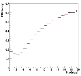
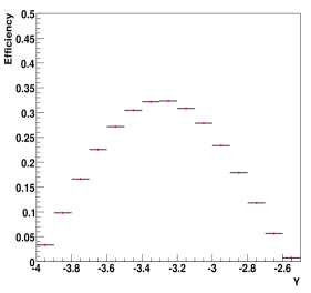
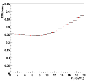
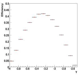
Figure 3.13: $p_{\mathrm{t}}$ (left) and $y$ (right) detection probabilities for J/$\psi$ (top) and $\Upsilon$ (bottom). The $p_{\mathrm{t}}$ detection probabilities are calculated in the Muon Spectrometer rapidity acceptance ($-4.0<y<-2.5$).

Quarkonia yields were computed for a data taking scenario of one year of pp data taking (assumed to be equivalent to $10^{7}$ s) at a luminosity of $3\times 10^{30}\,\mbox{${\rm cm}^{-2}{\rm s}^{-1}$}$ (cf. [9]).

The resulting $\mu^{+}\mu^{-}$ invariant mass distributions are shown in Fig. 3.14, both for the J/$\psi$ and $\Upsilon$ regions. As seen, all charmonium and bottomonium states are clearly resolved.

Together with quarkonia, all sources contributing to the $\mu^{+}\mu^{-}$ invariant mass continuum were taken into account, including muons from correlated and uncorrelated decay of $\mathrm{c\overline{c}}$ and $\mathrm{b\overline{b}}$ pairs and from the decay of $\pi$ and $K$. The invariant mass dimuon continuum is dominated by correlated sources.

The quarkonia signal is extracted from the total distribution by means of an interpolation. For each onium state, a Gaussian function was used for the central part of the peak and two more Gaussian with variable width were added to describe the tails. The correlated continuum was parametrized with two Gaussian functions with variable width, describing the low and high invariant mass regions, respectively.

The total number of detected J/$\psi$ is of the order of $3\times 10^{6}$, while the statistics expected for $\Upsilon$ is about two orders of magnitude smaller ($3\times 10^{4}$). The yields for all quarkonia states are summarized in Table 3.3, where the corresponding signal to background ratios and significances are also given.

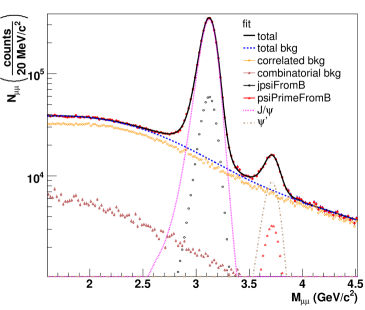
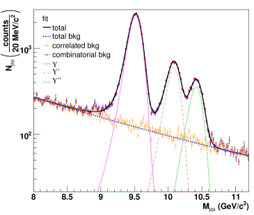
Figure 3.14: Opposite-sign dimuon mass spectra in pp collisions at $\sqrt{s}=14$ ${\rm TeV}$ for a running time of $10^{7}$ s at a luminosity of $3\times 10^{30}\,\mbox{${\rm cm}^{-2}{\rm s}^{-1}$}$. The J/$\psi$ and $\Upsilon$ mass regions are shown in the top and bottom panel respectively.

state	S ($\times 10^{3}$)	B ($\times 10^{3}$)	S/B	S/$\sqrt{S+B}$
J/$\psi$	2807	235	12.0	1610
$\psi^{\prime}$	75	120	0.62	170
$\Upsilon$	27.1	2.6	10.4	157
$\Upsilon^{\prime}$	6.8	2.0	3.4	73
$\Upsilon^{\prime\prime}$	4.2	1.8	2.4	55

Table 3.3: Expected quarkonia signal and background yields. Numbers refer to an interval corresponding to $\pm$ 1 FWHM around the resonance mass peak. Signal to background ratios and significances are also listed. All yields and significances are for a $10^{7}$ s running time with a luminosity of $3\times 10^{30}\,\mbox{${\rm cm}^{-2}{\rm s}^{-1}$}$.

The obtained statistics will be high enough to allow extracting the dimuon yields per bin of transverse momentum and rapidity. To this aim the transverse momentum (rapidity) of the detected opposite-sign muon pairs was computed and the complete sample of events was divided in several bins. For each $p_{\mathrm{t}}$ ($y$) bin, the corresponding dimuon invariant mass distribution was produced. From each of these distributions, the J/$\psi$ and $\Upsilon$ signals were extracted by fitting the invariant mass spectrum with the fitting procedure previously described. Then the raw number of detected resonances was corrected for the detection probability to obtain the differential cross section $\mathrm{d}\sigma/\mathrm{d}p_{\mathrm{t}}$ ($\mathrm{d}\sigma/{\mathrm{d}}y$). The obtained $\mathrm{d}\sigma/\mathrm{d}p_{\mathrm{t}}$ is normalized to the rapidity interval ($-4.0<y<-2.5$) covered by the Muon Spectrometer. The results in Fig. 3.15 (Fig. 3.16) show that the statistical error bars on the measured differential cross sections are small, in particular for the J/$\psi$, due to the high expected statistics.

For completeness the contribution of J/$\psi$ from B decay, though not directly measurable, is also shown in the left panels of both figures.

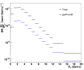
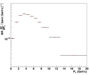
Figure 3.15: $BR_{\mu\mu}\mathrm{d}\sigma/\mathrm{d}p_{\mathrm{t}}$ for J/$\psi$ (left) and $\Upsilon$ (right) expected to be measured in a data taking time of $10^{7}$ s at a pp luminosity of $3\times 10^{30}\,\mbox{${\rm cm}^{-2}{\rm s}^{-1}$}$. The cross section is referred to the rapidity window $-4.0<y<-2.5$ covered by the Muon Spectrometer. The contribution of J/$\psi$ from B decay is also shown in the left panel.

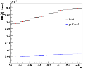
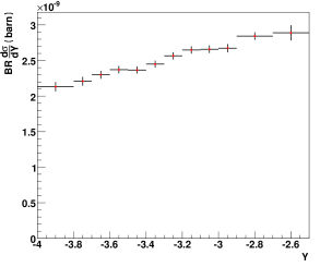
Figure 3.16: $BR_{\mu\mu}\mathrm{d}\sigma/{\mathrm{d}}y$ for J/$\psi$ (left) and $\Upsilon$ (right) measured in a data taking time of $10^{7}$ s at a pp luminosity of $3\times 10^{30}\,\mbox{${\rm cm}^{-2}{\rm s}^{-1}$}$. The contribution of J/$\psi$ from B decay is also shown in the left panel.

Leading order calculations show that in pp collisions at $\sqrt{s}=14$ ${\rm TeV}$, J/$\psi$’s with rapidity higher than 3.0 are produced by gluons carrying a fraction $x$ of the proton momentum lower than $10^{-5}$.

In such region, due to a lack of experimental data, the available gluon distribution functions rely on extrapolations, thus manifesting a significant disagreement. The feature is depicted in Fig. 3.17, showing a comparison between PDF sets calculated at Leading Order (LO) precision by different collaborations, namely Martin-Roberts-Stirling-Thorne (MRST98 [4] and MRST01 [10]) and the Coordinated Theoretical-Experimental Project on QCD (CTEQ5 [11] and CTEQ6 [12]): the $x$-values explored by J/$\psi$ in the ALICE Muon Spectrometer acceptance (in yellow) partially sits in the region of extrapolation. It is worth noting that, due to its larger mass, $\Upsilon$ production is sensitive to $x$-values larger than $10^{-5}$.

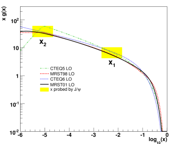
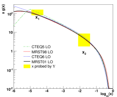
Figure 3.17: Comparison of the gluon distributions from MRST and CTEQ. $x$ regions probed by J/$\psi$ and $\Upsilon$ produced in pp collisions at $\sqrt{s}=14\mbox{${\rm TeV}$}$ in the rapidity region $-4.0<y<-2.5$ are shown.

Starting from the Color Evaporation Model as a guideline, it is possible to show that the J/$\psi$ rapidity distribution,

$$\frac{\mathrm{d}\sigma_{\scriptscriptstyle{J/\psi}}^{\scriptscriptstyle{CEM}}}{{\mathrm{d}}y}=\frac{F_{\scriptscriptstyle{J/\psi}}}{s}\sum_{i,j}{\int_{4m_{Q}^{2}}^{4m_{H}^{2}}{\mathrm{d}\hat{s}\,\hat{\sigma}_{ij}(\hat{s})f_{i/A}(\sqrt{\frac{\hat{s}}{s}}e^{y},\mu^{2})f_{j/B}(\sqrt{\frac{\hat{s}}{s}}e^{-y},\mu^{2})}}$$ (3.3)

is an observable sensitive to the PDF variation at low $x$.

This is done by making the following two approximations:

• in the elementary cross section $\hat{\sigma}_{ij}$, only the dominant contribution $gg\rightarrow\,$$Q\bar{Q}$ is taken into account

• both the elementary cross section $\hat{\sigma}_{gg}$ and the gluon distributions are taken at leading order

The calculation was carried out with different PDFs. The results are summarized by the curves in Fig. 3.18. We note that the rapidity distributions shown in this figure are normalized by setting equal to unit their integral from -4.0 to -2.5 rapidity units. This way of presenting the results emphasizes the fact that different behaviors of the gluon distribution functions at low $x$ (see Fig. 3.17) lead to different shapes of the J/$\psi$ rapidity distribution (see Fig. 3.18) in the interval covered by the muon spectrometer.

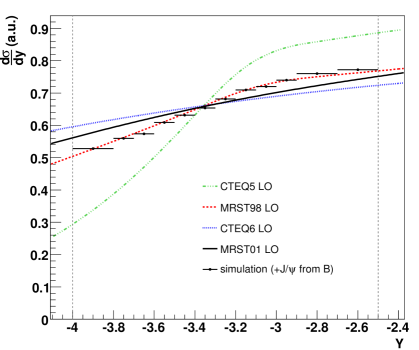
Figure 3.18: Comparison between J/$\psi$ rapidity distributions obtained with four different PDF sets (area in detector acceptance is normalized to 1). Simulation results are also shown.

Such behavior can be easily understood by analyzing Eq. 3.3. The rapidity distribution depends on:

• the product of parton distribution functions

• the elementary cross section $\hat{\sigma}_{gg}(\hat{s})$

• the ratio $F_{\mbox{J\kern-0.35002pt/\kern-0.35002pt$\psi$}}/s$ (assumed to be constant in the model)

The last term only affects normalization. Hence the shape of the distribution is related only to the first two quantities. However, since the elementary cross section doesn’t depend explicitly on $y$ and it is not expected to give rise to large variation of magnitude in the small range of integration ($4m_{Q}^{2}<\hat{s}<4m_{H}^{2}$), one can conclude that the shape of the distribution is mainly dependent on PDFs.

The possibility of focusing the study on the shape of the rapidity distribution, disregarding the absolute normalization, is extremely favorable from the experimental point of view, since lots of systematic errors (e.g. on luminosity, global acceptance effects, etc.) do not enter.

The next (and last) step of the study presented here is aimed to show that the accuracy of data collected with the Muon Spectrometer will be good enough in order to resolve the different rapidity distributions.

A direct comparison with the simulation results in Fig. 3.16 is not possible, since such data were obtained by adopting the MRST98 set computed at NLO, while the calculations presented in this section concern LO quantities. Hence the J/$\psi$ rapidity distribution was re-obtained from simulation after adopting MRST98 LO as input. Such distribution (the simulation points in Fig. 3.18), is then compared with the calculations with different PDF sets (curves in Fig. 3.18). It is worth noting that, differently from calculations, the simulated data already include contribution from B decay, which slightly change the shape of the distribution. However the change is limited as it can be seen by comparing simulated data and the calculation of prompt J/$\psi$ distribution obtained with the same PDF set (red curve of Fig. 3.18). This figure shows that, due to the high statistics, the accuracy of the data that are expected to be collected by the ALICE Muon Spectrometer will be good enough to allow to discriminate among different gluon distribution functions in the region of $x<10^{-5}$ (at least in the frame of a leading order analysis).

Parton Densities at the LHC

A. Tricoli

4.22 Introduction

The start up of the LHC machine is now imminent and theorists and experimentalists are converging their efforts to enhance the LHC discovery potential. This implies minimising theoretical and experimental uncertainties. Among the theoretical uncertainties the knowledge of the proton structure plays a major role: the accurate evaluation of parton density functions (PDF’s) is vital to provide reliable predictions of new physics signals (i.e. Higgs, Supersymmetry, Extra Dimensions etc.) and their background cross sections at the LHC. As shown in the contribution by C. Mariotti, E. Migliore and P. Nason , at hadron colliders the inclusive cross section for hard production processes is the convolution of the cross section at parton level, calculable at fixed order in perturbation theory, and the parton densities of the two interacting partons.

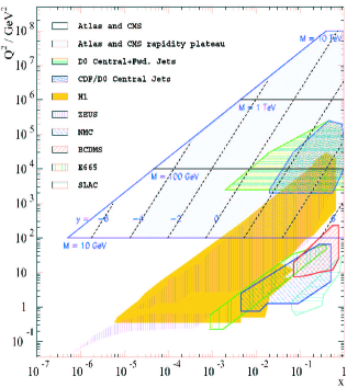
Figure 4.19:

The $Q^{2}$-$x$ kinematic plane for the LHC and previous experiments, showing the mass ($M$) and rapidity ($y$) dependence.

Our knowledge of the proton structure is improving fast thanks to more experimental data being available and thanks to more precise and sophisticated theoretical calculations: PDF’s are nowadays available up to the next-to-next-to leading order (NNLO) in perturbative QCD and in recent years they have been also providing uncertainties which take into account experimental systematic errors and the correlations between data points that enter the global fits. Despite the great improvement on PDF’s in recent years, their uncertainty dominates many cross section calculations for the LHC. As visible in fig. 4.19, the LHC will probe kinematic regions in $x$ (parton momentum fraction) and $Q^{2}$ (hard scattering scale) never explored before, such as the $very~{}high$-$Q^{2}$ and the $very~{}low$-$x$ regions. At low-$x$ the current theoretical formalism (DGLAP) is at the edge of its supposed applicability. For the production of $Z$ and $W$ bosons the participating partons have small momentum fractions at central rapidity, $x\sim 10^{-3}$, and in the whole measurable rapidity region, $|y|<2.5$, they are within the range $10^{-4}<x<0.1$. Thus, at the electro-weak scale the theoretical predictions for the LHC cross sections are dominated by low-$x$ PDF uncertainty. At the ${\rm TeV}$ scale, where we expect new physics, the interacting partons have higher momentum fractions and very high $Q^{2}$ ($\geq 10^{6}~{}{\rm GeV^{2}}$). Thus, at the ${\rm TeV}$ scale the cross section predictions are dominated by high-$x$ PDF uncertainty and rely on the extrapolation of the DGLAP equations. In both kinematic regimes the gluon density, which is in most regions the less well constrained density function, plays a major part: at low $x$ the gluon density dominates the quark and anti-quark densities, at high $Q^{2}$ the interacting partons get an important contribution from the sea, which is driven by the gluon density, via the $g\rightarrow q\bar{q}$ splitting process. For a review on hard interactions of quarks and gluons at the LHC refer to [1].

Past and running experiments, such as HERA, have been providing vital information to improve our knowledge of the parton densities, however the broad kinematic region of the LHC forces (and offers a unique opportunity to) ATLAS and CMS experiments to use their own data to constrain the parton densities, in particular the gluon, in the kinematic regions where they are not sufficiently well determined. In section 4.25 it will be shown that significant improvement on PDF fits can be made with LHC data.

4.23 Global fits and error analysis

Perturbative QCD provides the evolution equations for the parton densities, DGLAP equations, but does not provide us with their analytic forms as function of $x$. The most common approach to extrapolate PDF’s as function of $x$ and $Q^{2}$ consists in solving the DGLAP equations by parameterising the parton densities $q_{i}(x)$ at a fixed scale $Q^{2}_{0}=1-7~{}{\rm GeV^{2}}$, applying assumptions and constraints derived from theory and measurements. Then, with the DGLAP equations, we numerically extrapolate the values of $q_{i}(x,Q^{2})$ to different values of $Q^{2}$ and a global fit of experimental data is performed. For valence quarks the parameterisations have usually this behaviour $q_{V}\approx x^{\lambda}(1-x)^{\eta}$, whereas for the gluon and sea quarks they are of this kind $q_{S}(g)\approx x^{-\lambda}(1-x)^{\eta}$. However there is no unanimous agreement on the parametric functions to use and on the number of free parameters. For a review refer to [2].

Different regions in the $x,Q^{2}$ plane and also different partonic components are probed by the available world experimental data. These include DIS data from fixed target experiments and HERA, Drell-Yan data, inclusive jet production and $W$ charge asymmetry from Tevatron.

There are various groups who are fitting the proton structure function data, among them CTEQ and MRST. Recent PDF sets include in their analyses up-to-date experimental data and attempt to provide coherent estimates of the uncertainties, including experimental correlated systematic errors. The differences between these PDF sets can be summarised in three categories: different choices of input data sets, different theoretical model assumptions and different error analyses.

There are many sources of uncertainty which contribute to a global fit uncertainty. These can have experimental and theoretical origins. The former are related to the data errors which enter the fit, the latter are due to the model uncertainties of the theoretical framework. The theoretical uncertainties concern both the non-perturbative (parameterisations) and perturbative parts of the calculations: assumptions imposed to limit the number of free parameters, higher order truncations in the DGLAP formalism etc.

The treatment of the experimental uncertainties, especially the correlated systematic uncertainties, is a complex subject which is partly still under debate. A modified version of the standard $\chi^{2}$ method is used to take into account non-Gaussian systematic errors and their correlations: $\chi^{2}\rightarrow\tilde{\chi}^{2}+\Delta T^{2}$, where $\Delta T$ is the so-called “tolerance”, a complicated mathematical expression that includes correlated systematic terms [2]. There are then two methods to compute the central values of the theoretical PDF parameters and their uncertainties: the offset and the Hessian method. In the offset method the correlated systematic errors affect only the determination of the PDF uncertainty, not the best fit. This method is used for ZEUS PDF’s. Conversely in the Hessian method, used by CTEQ and MRST groups, the collective effect of the correlated systematic errors has also an impact on the best fit.

For both, the offset and the Hessian methods, the PDF uncertainty is conventionally computed along the eigenvectors of the diagonalised covariance or Hessian matrices. The number of eigenvectors corresponds to the number of free parameters in the parton density parameterisations. Contemporary PDF sets provide a central value PDF set, corresponding to the best data fit, and two PDF sets for each uncertainty eigenvector, giving the upper and lower limit on the uncertainty. Given a PDF set, the upper limit of the PDF uncertainty is calculated for a physical observable by adding in quadrature the upward displacement eigenvectors, whereas the lower limit by adding in quadrature the downward displacement eigenvectors. MRST group has chosen 15 free parameters, leading to 30 error sets; CTEQ6 has 20 free parameters and 40 error sets. Fig. 4.20 shows CTEQ6.5 fit for all parton densities at the scale $Q^{2}\sim M_{W}^{2}$ and its gluon uncertainty compared to the MRST2004NLO gluon best fit.

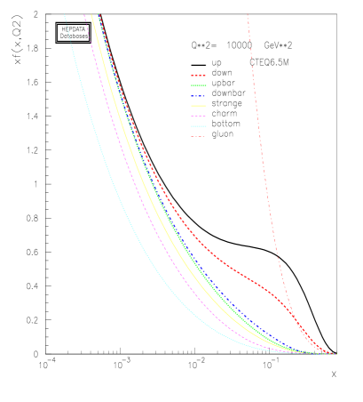
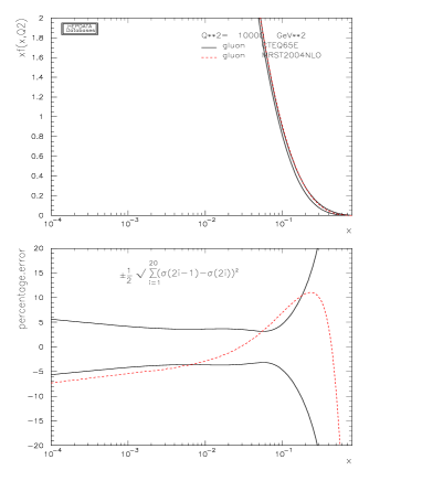
Figure 4.20:

Left: CTEQ6.5M set at $Q^{2}\sim M_{W}^{2}$. Right: comparison between CTEQ6.5M (black) and MRST2004NLO (red) gluon PDF’s and their uncertainties.

4.24 Impact of PDF uncertainty on LHC physics

The experience from previous experiments teaches that the PDF uncertainties must be properly taken into account or features of the SM physics can be misinterpreted as evidence of new physics. For example an unexplained discrepancy between data and theory was originally found in the Tevatron Run-I jet data, which was subsequently reabsorbed within the theoretical uncertainty when a more accurate PDF error analysis was performed.

G. Polesello’s contribution on inclusive jet cross-section has shown that the PDF uncertainty is dominating for high $E_{T}$ jets over the renormalisation/factorisation scale and the experimental energy scale uncertainties: $10\%$ at $1~{}{\rm TeV}$, $25\%$ at $2~{}{\rm TeV}$, $60\%$ at $5~{}{\rm TeV}$.

Extra dimensions

In extra dimensions models, if the compactification scale $M_{C}$ is about few TeV, it is possible to observe the production of gravitons and Kaluza Klein (KK) excitations at the LHC. If gauge bosons can propagate in the extra dimensions, we also expect a violation of the SM logarithmic behaviour of the running couplings. In this scenario, if we consider the CTEQ6M PDF uncertainty on the di-jet cross-section, we see the extra dimensions prediction being absorbed within the SM prediction zone: the high-$x$ gluon uncertainty can cause a decrease of the discovery reach from $M_{C}=5~{}(10)~{}{\rm TeV}$ to $M_{C}<2~{}(3)~{}{\rm TeV}$, depending on the number of extra dimensions [3].

Higgs

The accurate measurements of the Higgs production cross sections and decay branching ratios are crucial to explore all Higgs boson fundamental properties. At the same time, we need very precise estimates of the various theoretical uncertainties.

It is found that the PDF uncertainty can be of the same order of magnitude or even higher than the other theoretical uncertainties. In fact the perturbative calculations of Higgs production cross section are becoming more stable as higher orders are included, leaving the PDF uncertainty as one of the largest contributions to the total theoretical uncertainty. For example for the dominant Higgs production channel, $gg\rightarrow H$, the PDF uncertainty on $gg$ luminosity, can be larger than the factorisation and renormalisation scale uncertainty: in fact the differences in the $gg$ luminosity prediction between MRST2002 and Alekhin2002 can be higher than $10\%$ for low Higgs mass scenarios. Furthermore, studying the effect of three different PDF sets (i.e. CTEQ6M, MRST2001E and Alekhin2002) with their quoted uncertainties, on various Higgs productions channels, we see that the PDF uncertainty can be of the order of $\sim 10-15\%$ on the production cross-section [4].

High mass Drell-Yan

Several new physics models predict events with two charged leptons originating from the decay of a massive object. A peak in the $d\sigma/dM$ distribution is a clean signature of a new resonance: the identification and reconstruction of high-mass di-lepton final states can be done with high efficiency and the SM background can be small. However the shape and normalisation of the predicted observable distributions depend on PDF and its uncertainty.

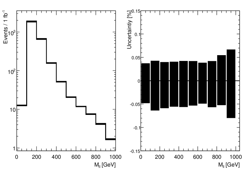
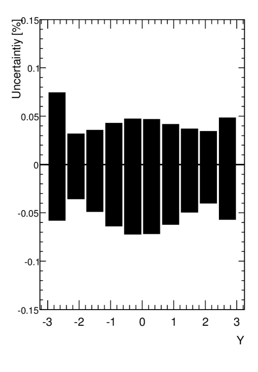
Figure 4.21:

CTEQ6.1 uncertainty on distributions of the high-mass di-electron $M_{ll}$ (left and centre) and rapidity $y$ (right). Herwig+Jimmy generation and ATLAS full simulation [5]. N.B.: the drop in the low $M_{ll}$ spectrum is an artifact of the event selection in the Monte Carlo.

In fig. 4.21 we see the total CTEQ6.1 uncertainty on the distributions of the reconstructed rapidity $y$ and invariant mass $M_{ll}$ of the lepton pair: 40 CTEQ error sets have been accounted for, applying the PDF reweighting technique (see sec. 4.26). The uncertainty is in the range $4-7\%$ on both $y$ and $M_{ll}$ up to $1~{}{\rm TeV}$. Excluding the bins at the edge of the rapidity distributions, where statistical fluctuations are present, we see that the largest PDF uncertainty is at $y\sim 0$. As explained in [5], a study shows that NLO QCD corrections, applied on Monte Carlo (MC) and on PDF, enhance the cross section with respect to the LO prediction by $24-36\%$, with the largest NLO corrections at $y\sim 0$. A discrepancy of about $6\%$ is found between MRST-NLO and CTEQ-NLO PDF’s.

4.25 How to constrain PDF at LHC

Several Standard Model processes are under study to constrain parton densities: $\gamma$, $W$ and $Z$ boson and inclusive jet production processes are equally important to constrain the parton densities and in particular the gluon density in complementary kinematic regions (see [6]).

In G. Polesello’s contribution we appreciate how the LHC jet data can be used to better constrain PDF fits: if the experimental systematic uncertainty is under control to $\leq 10\%$ level, LHC jet data can significantly contribute to constraining the high-$x$ gluon density with $1~{}fb^{-1}$ luminosity. Other studies [7] have also shown that the prompt photon production process is extremely sensitive to PDF differences and can probe the perturbative theory of the gluon at high-$x$: the discrepancy between MRST2004-NLO, CTEQ6.1M and older PDF sets can be of the order of $16-18\%$ on the photon $\eta$ and $p_{\scriptscriptstyle T}$ distributions.
Furthermore, the $bg\rightarrow Zb$ process is sensitive to the $b$-quark content of the proton and the LHC predictions for the $Z+b$ cross-section, using different PDF sets, are $\pm 5-10\%$ [8].

4.25.1 W rapidity distributions

A few days of LHC running at the nominal low luminosity ($10^{33}{\rm cm^{-2}s^{-1}}$) are sufficient to make the statistical uncertainty negligible with respect to the systematic uncertainties on $W$ cross section. Among the systematic uncertainties there are experimental and theoretical contributions.

The ATLAS strategy for selecting $W$ bosons consist of identifying an isolated and highly energetic lepton, $E_{\scriptscriptstyle T}>25~{}{\rm GeV}$, and requiring a large amount of missing energy in the event due to the neutrino escaping detection, $\hbox to0.0pt{\hbox to7.95831pt{\hfil/\hfil}\hss}E_{T}>25~{}{\rm GeV}$. The analysis of $W\rightarrow e\nu_{e}$ events fully simulated in the ATLAS detector, in the early data scenario, shows that the $W$ boson is a very clean signature: the trigger and the electron off-line identification with the electron $E_{\scriptscriptstyle T}$ and $\hbox to0.0pt{\hbox to7.95831pt{\hfil/\hfil}\hss}E_{T}$ cuts leave a background contamination dominated by QCD events (less than $5\%$) and $W\rightarrow\tau\nu_{\tau}$ (about $0.5\%$). If a jet veto cut is added, the QCD background can be further reduced to a level of $\leq 1\%$ [9]. Therefore the $W$ sector is an ideal environment to study and constrain theoretical and experimental systematics.

Higher order corrections

The differential cross section $d\sigma/dy$ for $W$ production has been calculated to the NNLO order in QCD with an energy scale uncertainty of $\leq 1\%$ [10]. With this level of precision in perturbative QCD calculations, the electro-weak (EW) contributions are no more negligible. As presented in this workshop, leading order electro-weak contributions with multi-photon radiation introduce corrections of the order of few percent on $W$ boson cross-sections. The EW corrections, computed by the program HORACE interfaced to HERWIG in the $\alpha(0)$ scheme in the muon channel [11], are constant in rapidity and are about $3.5\%$ for a cut on the muon transverse momentum of $p_{\scriptscriptstyle T}>25~{}{\rm GeV}$ and can be up to $5.2\%$ for loser $p_{\scriptscriptstyle T}$ cuts. The dependence on the muon charge is negligible (up to $0.4\%$ for lose $p_{\scriptscriptstyle T}$ cuts) [12]. Considering that these corrections in the muon channel are flat in rapidity and negligible on the muon-charge asymmetry, we can state that they do not have an impact on the PDF extraction, however they are relevant for luminosity measurements in order to achieve a precision of $6\%$ or better. The electron channel needs further investigation.

PDF uncertainty on $W^{\pm}$ rapidity distribution.

From fig. 4.22 we can see the full PDF uncertainties for three different PDF analyses, on the rapidity distribution of $e^{\pm}$ originating from $W^{\pm}$ decays. Their predictions are compatible within their uncertainties, which are in the range $4\%-12\%$, and are dominated by the gluon density.

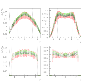
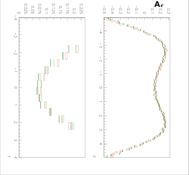
Figure 4.22:

HERWIG simulations of $e^{\pm}$ from $W^{\pm}$ decay, with CTEQ6.1M (red), MRST2001 (black) and ZEUS-S (green) PDF’s and their quoted uncertainties (estimated with the PDF reweighting technique as in sec. 4.26). The top plots are at generator level, the bottom plots at ATLFAST detector level. Left fig: $e^{-}$ (left plots) and $e^{+}$ (right plots) rapidity spectra with NLO-QCD corrections. Right fig: electron-charge asymmetry [13].

In a previous paper [14] it is demonstrated that the LHC can improve the current constraint on the low-$x$ gluon parameter $\lambda_{g}$ ($xg(x)\approx x^{-\lambda_{g}}$) by more than $41\%$ by fitting the $e^{+}$ and $e^{-}$ rapidity distributions, if their experimental systematic uncertainties are kept under $5\%$ level.

In the lepton-charge asymmetry $A_{l}=(\frac{d\sigma}{d\eta}^{l^{+}}-\frac{d\sigma}{d\eta}^{l^{-}})/(\frac{d\sigma}{d\eta}^{l^{+}}+\frac{d\sigma}{d\eta}^{l^{-}})$ most of the gluon uncertainty cancel out leaving the valence up ($u_{V}$) and down ($d_{V}$) densities as main contributions to the total PDF uncertainty, which is reduced to $\sim 5\%$ at $\eta\approx 0$. However a discrepancy of $\sim 15\%$ is present at $\eta\approx 0$ between the MRST2002 and other two PDF’s, CTEQ6.1M and ZEUS-S [15]. In fact the MRST PDF’s prediction for $u_{V}-d_{V}$ valence density is different from the other PDF’s and is outside the quoted PDF uncertainty bands. This difference in current PDF fits comes from the lack of data on valence quantities at such low-$x$. The LHC can be the first experiment to perform such measurement in the kinematic region $x\approx 10^{-3}$ and $Q^{2}=M_{W}^{2}$.

A posteriori inclusion of PDF’s in NLO calculations.

The MC computation of QCD final state observables to NLO is a lengthy process. In order to study the impact of PDF uncertainties on QCD cross section measurements in a faster way and allow for PDF fitting of these quantities, the technique of “a posteriori” inclusion of PDF’s in NLO calculations has been developed for LHC processes [16] [17]. A MC run is used to generate a grid (in $x_{1}$, $x_{2}$ and $Q$) of cross section weights that can subsequently be combined with an arbitrary PDF set. This enables the decoupling of the lengthy calculation of perturbative MC weights from the convolution with the parton densities. Perturbative coefficients for jet (using NLOJET++), W and Z boson (using MCFM) production processes can be collected on a grid with an accuracy better than $0.02\%$.

4.26 PDF reweighting of Monte Carlo events

The computation of the full PDF uncertainty on a physics process is a cumbersome procedure. Given one PDF set, such as CTEQ or MRST, it requires the generation of twice as many MC samples as the number of free parameters in the global fit. Furthermore one error analysis might not be sufficient since, as seen above, there can be large discrepancies between the results of different error analyses.

A PDF reweighting technique has been studied and tested, requiring only one Monte Carlo generation with one conventional PDF set   [13][14].

This technique has been implemented using hard process parameters of the MC generation: flavours ($flav_{1}$ and $flav_{2}$) and momentum fractions of the interacting partons $x_{flav_{1}}$, $x_{flav_{2}}$ and the energy scale $Q$. The PDF set used for the MC generation is named $PDF_{1}$.

The PDF reweighting technique consists of evaluating, on the event-by-event basis, the probability of picking up the same flavoured partons with the same momentum fractions $x_{flav_{1}}$, $x_{flav_{2}}$, according to a second PDF set, $PDF_{2}$, at the same energy scale $Q$, then evaluating the following ratio

$$Event~{}Weight=\frac{f_{PDF_{2}}(x_{flav_{1}},Q)}{f_{PDF_{1}}(x_{flav_{1}},Q)}\cdot\frac{f_{PDF_{2}}(x_{flav_{2}},Q)}{f_{PDF_{1}}(x_{flav_{2}},Q)}~{}.$$ (4.4)

After the $Event~{}Weight$ is applied on MC events generated with $PDF_{1}$, they will effectively be distributed according to $PDF_{2}$.

This technique has been tested using HERWIG (for inclusive W production) and ALPGEN interfaced to HERWIG (for W+jets production) as Monte Carlo generators and with various recent PDF sets. Similar results have been obtained with these two MC generators and with different PDF sets, as discussed below.

Figure 4.23:

Left fig: $W^{-}$ and $W^{+}$ rapidity distributions at HERWIG generator level for events generated with CTEQ6.1M (dashed lines) and for events generated with MRST2002 (solid lines) and their relative differences (at the bottom). The straight lines are the means of the points with uncertainty bands. Right fig: same as left hand side plots for events generated with CTEQ6.1M (dashed lines) and for events generated with MRST2002 and PDF-reweighted with CTEQ6.1 (solid lines). Similar results have been obtained reweighting between MRST2002 and ZEUS-S PDF’s.

Fig. 4.23 shows the accuracy of this technique using HERWIG: the bias over the all $y$ range is of the order of $0.5\%$ or less and there is no evidence of $y$ dependence. Comparing the bottom plots on the right and left hand sides of fig. 4.23 we see that the PDF reweighting technique corrects for the difference in normalisation between $PDF_{1}$ and $PDF_{2}$ and corrects for the $y$ modulation.

This technique can be used to estimate the full PDF uncertainty, starting from one sample of MC generated events, for distributions that are determined by the MC hard process.

NNLO Evolution of the Pdf’s and their Errors: Benchmarks and Predictions for Drell-Yan

Alessandro Cafarella, Claudio Corianò, Marco Guzzi

Abstract

We quantify the impact of the next-to-next-to-leading order evolution on the Drell-Yan total cross section and on the corresponding rapidity distributions of the lepton pair and compute the corresponding errors. We base our analysis on Candia, a program that solves the DGLAP equations using the method of the $x$-space iterates.

5.27 Introduction

In the search for new physics at the LHC we need high precision in the determinations of the QCD background, possibly at next-to-next-to-leading order (NNLO) in the strong coupling constant $\alpha_{s}$. While it is expected that only a few processes will be computed in the near future at this order of accuracy in QCD, for Drell-Yan lepton pair production, some of these corrections - for instance those involving the invariant mass distributions - have been available for some time [1]. The study of this process will be essential both in the search of extra neutral interactions and for partonometry, where the impact of the perturbative resummation [2] can be studied in detail given the large number of events expected at the LHC. More recently, following the computation of the invariant mass distribution $d\sigma/dQ$, where $Q^{2}$ is the invariant mass of the lepton pair, also the rapidity distributions $d\sigma/(dYdQ)$, implemented in VRAP [3] have been computed. A fully exclusive numerical computation has also been presented [4]. Next-to-leading order (NLO) analysis of the forward-backward asymmetries $A_{FB}$ on the Z resonance and NNLO charge asymmetries have also been determined [3]. The computation of the hard scatterings for some of these processes has been performed much before that the analytical computation of the NNLO evolution kernels needed for a consistent extraction of NNLO parton distributions (pdf’s) were available. Following the computation of the kernels [5], some benchmarks for the NNLO evolution have been presented [6], followed by a later update [7].

Testing the benchmarks by using independent approaches that solve the equations is not only a demanding numerical problem, but involves subtle issues concerning the types of solutions that are implemented in a given numerical algorithm. Specifically, we have shown in [8, 9] that the selection of a given ansatz - either in Mellin space or in x-space - in the solution of the DGLAP involves a specific arrangement of the logarithmic expansion that solves iteratively the equations. For instance, ansatze for the exact solutions perform automatically a resummation of the contributions identified by the simplest logarithmic ansatz (also called “truncated solutions”). These involve logarithms of the ratio of two couplings $\log(\alpha_{s}(Q^{2})/\alpha_{s}(Q_{0}^{2}))$ at two different scales $Q$ and $Q_{0}$. Exact solutions, instead, replace these logarithmic expansions with more complicated functions of $\alpha_{s}$. Details can be found in [8, 9, 10].

These expansions apply generically both to forward and non-forward twist-2 operators, and converge to the solutions of the evolution equations with very high precision. Concerning the structure of the evolution codes, these are usually based either on the numerical Mellin inversion (using an ansatz in moment space) or on “brute force methods”. In this second case the numerical solution is built by a discretization of the equations, reduced to a stable finite-difference scheme. The theoretical indetermination coming from the various approaches, as we have pointed out in [9], has to do with the the selected accuracy of the solution.

5.28 The choice of the solution and the theoretical indetermination

We have re-analized the issue of the initial state dependence of the predictions for the $d\sigma/dQ$ and $d\sigma/(dydQ)$ cross sections in [9, 10], focusing our attention near the $Z_{0}$ peak.

Being the predictions coming from the inclusions of the NNLO corrections quite small, it is natural to worry whether the errors coming from the statistical fits in the determination of the pdf’s to the experimental data and the indeterminations due to the treatment of the evolution can be compared so that the size of the errors claimed in the hadronic cross sections are quantified consistently. We point out that the specific choice of the solution of the evolution equation brings in an intrinsic indetermination which is comparable with the error coming from the fits to the pdf’s. This indetermination is of theoretical origin.

In our analysis we will omit most of the theoretical details that can be found in [10] and come to a discussion of the numerical results, since these can be of interest for actual experimental searches. We also present some benchmarks for the NNLO evolution that can be useful for a consistent comparison with other codes. An extensive numerical analysis of the predictions on the Z resonance that illustrates the points summarized here can be found in [9].

As we are going to see, the variations induced by the choice of the solution of the DGLAP induce variations on the cross section of the order of $1\%$ or so at NNLO, and clearly affect also the NNLO $K$-factor for the total cross section. We have used for this study Candia [8], which implements the truncated and exact solutions of the DGLAP built without the numerical Mellin inversions. On the countrary of other programs that need initial conditions of a specific functional form, Candia allows any initial conditions to be studied, being based on x-space algorithms. An extended version of Candia, called $\textsc{Candia}_{\textsc{DY}}$ allows to study the invariant mass distribution to NNLO. An interface with VRAP is also under development.

(a) Alekhin Evolution

(b) MRST Evolution

Figure 5.24: Cross Sections in the region of the peak of the Z boson at LO, NLO, and NNLO obtained using the luminosities evolved respectively by Alekhin and MRST

5.29 Benchmarks and Numerical Results

Now, we come to illustrate a comparison between the NNLO evolution performed by Candia and Pegasus [11], using the initial conditions of the Les Houches model. This model works as a benchmark and allows to compare various evolution codes. We show the behaviour of the gluon distribution and the valence up quark distribution (non-singlet). We observe that the differences in the singlet case are around $0.4-0.3\%$ or less, while for the valence up quark they are around $3\%$ at $x=10^{-5}$ and then decrease to $0.1-0.02\%$ at $x=0.1$ (see Table 5.4). We have denoted with $x\delta f(x)$ the relative differences normalized to the Pegasus determination, i.e. $x\delta f(x)\equiv(xf(x)_{\textsc{Pegasus}}-xf(x)_{\textsc{Candia}})/xf(x)_{\textsc{Pegasus}}$. We have set the factorization and renormalization scales to coincide and equal to $Q=100$ GeV. In Candia we have used the “asymptotic solutions”, which are similar to those obtained by PEGASUS in one of its 3 running modes. The two algorithms and their implementations compare very well in the x-region relevant for the LHC (around $0.1\%$ at NNLO). Using the same benchmark we have calculated the NNLO cross sections using the two evolutions (see Tab. 5.5), and we observe that the differences between the two methods in the kinematical region that we are considering are around $0.2-0.3\%$.

Candia vs Pegasus PDFs at NNLO, Les Houches input, VFN scheme, $Q=\mu_{F}=\mu_{R}=100$ GeV
$x$	$xg(x)^{\textsc{Candia}}_{asymp}$	$xg(x)^{\textsc{Pegasus}}$	$\delta xg(x)$	$xu_{v}(x)^{\textsc{Candia}}_{asymp}$	$xu_{v}(x)^{\textsc{Pegasus}}$	$\delta xu_{v}(x)$
$1e-05$	$2.1922\cdot 10^{+2}$	$2.2012\cdot 10^{+2}$	$4.1108\cdot 10^{-3}$	$3.0823\cdot 10^{-3}$	$3.1907\cdot 10^{-3}$	$3.3962\cdot 10^{-2}$
$0.0001$	$8.8486\cdot 10^{+1}$	$8.8804\cdot 10^{+1}$	$3.5856\cdot 10^{-3}$	$1.3871\cdot 10^{-2}$	$1.4023\cdot 10^{-2}$	$1.0811\cdot 10^{-2}$
$0.001$	$3.0319\cdot 10^{+1}$	$3.0404\cdot 10^{+1}$	$2.8106\cdot 10^{-3}$	$6.0060\cdot 10^{-2}$	$6.0019\cdot 10^{-2}$	$6.9117\cdot 10^{-4}$
$0.01$	$7.7785\cdot 10^{+0}$	$7.7912\cdot 10^{+0}$	$1.6326\cdot 10^{-3}$	$2.3287\cdot 10^{-1}$	$2.3244\cdot 10^{-1}$	$1.8584\cdot 10^{-3}$
$0.1$	$8.5284\cdot 10^{-1}$	$8.5266\cdot 10^{-1}$	$2.1595\cdot 10^{-4}$	$5.4977\cdot 10^{-1}$	$5.4993\cdot 10^{-1}$	$2.9526\cdot 10^{-4}$
$0.2$	$2.4183\cdot 10^{-1}$	$2.4161\cdot 10^{-1}$	$9.1195\cdot 10^{-4}$	$4.8313\cdot 10^{-1}$	$4.8323\cdot 10^{-1}$	$2.0148\cdot 10^{-4}$
$0.3$	$7.9005\cdot 10^{-2}$	$7.8898\cdot 10^{-2}$	$1.3515\cdot 10^{-3}$	$3.4629\cdot 10^{-1}$	$3.4622\cdot 10^{-1}$	$1.9857\cdot 10^{-4}$
$0.4$	$2.5636\cdot 10^{-2}$	$2.5594\cdot 10^{-2}$	$1.6452\cdot 10^{-3}$	$2.1711\cdot 10^{-1}$	$2.1696\cdot 10^{-1}$	$6.7488\cdot 10^{-4}$
$0.5$	$7.6538\cdot 10^{-3}$	$7.6398\cdot 10^{-3}$	$1.8314\cdot 10^{-3}$	$1.1883\cdot 10^{-1}$	$1.1868\cdot 10^{-1}$	$1.2434\cdot 10^{-3}$
$0.6$	$1.9439\cdot 10^{-3}$	$1.9401\cdot 10^{-3}$	$1.9844\cdot 10^{-3}$	$5.4753\cdot 10^{-2}$	$5.4652\cdot 10^{-2}$	$1.8520\cdot 10^{-3}$
$0.7$	$3.7162\cdot 10^{-4}$	$3.7080\cdot 10^{-4}$	$2.2059\cdot 10^{-3}$	$1.9537\cdot 10^{-2}$	$1.9486\cdot 10^{-2}$	$2.6105\cdot 10^{-3}$
$0.8$	$4.1248\cdot 10^{-5}$	$4.1141\cdot 10^{-5}$	$2.5990\cdot 10^{-3}$	$4.4306\cdot 10^{-3}$	$4.4148\cdot 10^{-3}$	$3.5750\cdot 10^{-3}$
$0.9$	$1.1766\cdot 10^{-6}$	$1.1722\cdot 10^{-6}$	$3.7723\cdot 10^{-3}$	$3.3696\cdot 10^{-4}$	$3.3522\cdot 10^{-4}$	$5.1816\cdot 10^{-3}$

Table 5.4: NNLO pdf’s determined with Candia and Pegasus using the Les Houches model.

$\textrm{d}\sigma_{NNLO}/\textrm{d}Q$ [pb/GeV]. Candia vs Pegasus with Les Houches input.
$Q~{}[\textrm{GeV}]$	$\sigma_{NNLO}^{\textsc{Candia}}$	$\sigma_{NNLO}^{\textsc{Pegasus}}$	$\delta\sigma_{NNLO}$
$50.0000$	$8.0734\cdot 10^{+0}$	$8.1044\cdot 10^{+0}$	$3.8288\cdot 10^{-3}$
$60.0469$	$4.8771\cdot 10^{+0}$	$4.8948\cdot 10^{+0}$	$3.6106\cdot 10^{-3}$
$70.0938$	$4.4033\cdot 10^{+0}$	$4.4184\cdot 10^{+0}$	$3.4110\cdot 10^{-3}$
$80.1407$	$8.9241\cdot 10^{+0}$	$8.9527\cdot 10^{+0}$	$3.1936\cdot 10^{-3}$
$90.1876$	$3.3570\cdot 10^{+2}$	$3.3669\cdot 10^{+2}$	$2.9388\cdot 10^{-3}$
$91.1876$	$5.4905\cdot 10^{+2}$	$5.5067\cdot 10^{+2}$	$2.9299\cdot 10^{-3}$
$92.1876$	$3.3344\cdot 10^{+2}$	$3.3441\cdot 10^{+2}$	$2.8919\cdot 10^{-3}$
$120.0701$	$1.0249\cdot 10^{+0}$	$1.0274\cdot 10^{+0}$	$2.4285\cdot 10^{-3}$
$146.0938$	$2.8527\cdot 10^{-1}$	$2.8590\cdot 10^{-1}$	$2.1826\cdot 10^{-3}$
$172.1175$	$1.2295\cdot 10^{-1}$	$1.2319\cdot 10^{-1}$	$1.9887\cdot 10^{-3}$
$200.0000$	$6.0923\cdot 10^{-2}$	$6.1029\cdot 10^{-2}$	$1.7369\cdot 10^{-3}$

Table 5.5: NNLO cross sections in the two evolution methods.

(a) $K=\sigma_{NNLO}/\sigma_{NLO}$

(b) $K_{1}=\sigma_{NLO}/\sigma_{LO}$ and $K_{2}=\sigma_{NNLO}/\sigma_{LO}$

(c) $K_{1}=\sigma_{NLO}/\sigma_{LO}$ and $K_{2}=\sigma_{NNLO}/\sigma_{LO}$

(d) $K_{1}=\sigma_{NLO}/\sigma_{LO}$ and $K_{2}=\sigma_{NNLO}/\sigma_{LO}$

Figure 5.25: Various $K$-factors obtained with the evolution performed by Candia and MRST.

Coming to a description of the NNLO cross section obtained from a realistic model, we show in Tab. 5.6 results for the invariant mass distributions at $\sqrt{S}=14$ TeV according to Alekhin’s model [12]. Shown are also the errors which have been computed as discussed in [9]. A similar analysis has been performed using the MRST set [13] (see Tab. 5.8), for which the errors can be obtained, at this time, only at NLO.

The differences between our prediction and the MRST result for the total cross sections are around 1 per cent or below at LO, vary from $0.02\%$ to $0.3\%$ at NLO and are $2.6\%$ and below at NNLO (see Tab. 5.7). In this case the maximum difference has been found for $Q=50$ GeV. These differences, clearly, affect the values of the $K$-factors, as we are going to discuss below, which in our evolution are larger compared to those of MRST.

$\textrm{d}\sigma/\textrm{d}Q$ in [pb/GeV] for Alekhin with $Q^{2}=\mu_{F}^{2}=\mu_{R}^{2}$, $\sqrt{S}=14$ TeV
$Q~{}[\textrm{GeV}]$	$\sigma_{LO}$	$\sigma_{NLO}$	$\sigma_{NNLO}$
$50$	$6.22$ $\pm$ $0.27$	$7.48$ $\pm$ $0.24$	$7.43$ $\pm$ $0.21$
$60.04$	$3.72$ $\pm$ $0.15$	$4.50$ $\pm$ $0.13$	$4.49$ $\pm$ $0.12$
$70.1$	$3.30$ $\pm$ $0.12$	$4.03$ $\pm$ $0.11$	$4.05$ $\pm$ $0.10$
$80.1$	$6.65$ $\pm$ $0.24$	$8.20$ $\pm$ $0.24$	$8.19$ $\pm$ $0.23$
$90.19$	$253$ $\pm$ $8$	$313$ $\pm$ $9$	$309$ $\pm$ $8$
$91.19$	$415$ $\pm$ $14$	$514$ $\pm$ $15$	$506$ $\pm$ $15$
$120.07$	$0.80$ $\pm$ $0.02$	$0.99$ $\pm$ $0.02$	$0.96$ $\pm$ $0.03$
$146.1$	$0.225$ $\pm$ $0.006$	$0.277$ $\pm$ $0.007$	$0.269$ $\pm$ $0.007$
$172.1$	$0.097$ $\pm$ $0.002$	$0.119$ $\pm$ $0.003$	$0.117$ $\pm$ $0.003$
$200$	$0.047$ $\pm$ $0.001$	$0.058$ $\pm$ $0.001$	$0.058$ $\pm$ $0.001$

Table 5.6: Cross sections derived from the best fits for the 3 orders with their errors for the set by Alekhin.

$\textrm{d}\sigma_{NNLO}/\textrm{d}Q$ [pb/GeV]. Candia vs MRST evolution with MRST input, $\mu_{0}^{2}=1.25$ GeV2
$Q~{}[\textrm{GeV}]$	$\sigma_{NNLO}^{\textsc{Candia}}$	$\sigma_{NNLO}^{MRST}$	$\delta\sigma_{NNLO}$
$50.0000$	$6.4935\cdot 10^{+0}$	$6.6707\cdot 10^{+0}$	$2.6560\cdot 10^{-2}$
$60.0469$	$3.9997\cdot 10^{+0}$	$4.0961\cdot 10^{+0}$	$2.3534\cdot 10^{-2}$
$70.0938$	$3.6962\cdot 10^{+0}$	$3.7743\cdot 10^{+0}$	$2.0678\cdot 10^{-2}$
$80.1407$	$7.6755\cdot 10^{+0}$	$7.8198\cdot 10^{+0}$	$1.8455\cdot 10^{-2}$
$90.1876$	$2.9325\cdot 10^{+2}$	$2.9827\cdot 10^{+2}$	$1.6834\cdot 10^{-2}$
$91.1876$	$4.8006\cdot 10^{+2}$	$4.8822\cdot 10^{+2}$	$1.6702\cdot 10^{-2}$
$92.1876$	$2.9179\cdot 10^{+2}$	$2.9671\cdot 10^{+2}$	$1.6575\cdot 10^{-2}$
$120.0701$	$9.0411\cdot 10^{-1}$	$9.1687\cdot 10^{-1}$	$1.3918\cdot 10^{-2}$
$146.0938$	$2.5267\cdot 10^{-1}$	$2.5567\cdot 10^{-1}$	$1.1714\cdot 10^{-2}$
$172.1175$	$1.0938\cdot 10^{-1}$	$1.1049\cdot 10^{-1}$	$1.0028\cdot 10^{-2}$
$200.0000$	$5.4431\cdot 10^{-2}$	$5.4876\cdot 10^{-2}$	$8.1092\cdot 10^{-3}$

Table 5.7: NNLO cross section for Drell-Yan obtained by Candia using the MRST input and the evolved MRST pdf’s

$\textrm{d}\sigma/\textrm{d}Q$ in [pb/GeV] for MRST with $Q^{2}=\mu_{F}^{2}=\mu_{R}^{2}$, $\sqrt{S}=14$ TeV
$Q~{}[\textrm{GeV}]$	$\sigma_{NLO}$
$50$	$6.77$ $\pm$ $0.19$
$60.04$	$4.13$ $\pm$ $0.10$
$70.1$	$3.79$ $\pm$ $0.08$
$80.1$	$7.90$ $\pm$ $0.14$
$90.19$	$305$ $\pm$ $5$
$91.19$	$499$ $\pm$ $8$
$120.1$	$0.952$ $\pm$ $0.014$
$146.1$	$0.264$ $\pm$ $0.003$
$172.1$	$0.113$ $\pm$ $0.001$
$200$	$0.0556$ $\pm$ $0.0007$

Table 5.8: Cross sections derived from the best fits at NLO with the errors for the MRST set.

We have summarized in Fig. 5.25 four plots of the behavior of the 3 $K$-factors $K=\sigma_{NNLO}/\sigma_{NLO}$, $K_{1}=\sigma_{NLO}/\sigma_{LO}$ and $K_{2}=\sigma_{NNLO}/\sigma_{LO}$ obtained using Candia and the MRST evolution. These are shown as a function of $Q$, and evaluated at the center of mass energy of $\sqrt{S}=14$ TeV. The dependence of the results on the evolution is significant. In fact, from Fig. 5.25 it is evident that while the shapes of the plots of the $K$-factors are similar, there are variations of the order $2\%$, in the results using the two different evolutions. Both in the evolution performed with Candia and in the MRST evolution we use the same MRST input, choosing the initial scale $\mu_{0}^{2}=1.25$ GeV², and the same treatment of the heavy flavors. On the Z resonance we get

$$K(M_{Z})=(\hat{\sigma}_{NNLO}\otimes\Phi^{NNLO}_{MRST})/(\hat{\sigma}_{NLO}\otimes\Phi^{NLO}_{MRST})=0.97$$

$$K(M_{Z})=(\hat{\sigma}_{NNLO}\otimes\Phi^{NNLO}_{\textsc{Candia}})/(\hat{\sigma}_{NLO}\otimes\Phi^{NLO}_{\textsc{Candia}})=0.95$$

$$K(M_{Z})=(\hat{\sigma}_{NNLO}\otimes\Phi^{NNLO}_{Alekhin})/(\hat{\sigma}_{NLO}\otimes\Phi^{NLO}_{Alekhin})=0.98$$ (5.5)

which corresponds to a reduction by $2.7\%$ of the NNLO cross section compared to the NLO result, (MRST evolution) and larger for the Candia evolution, $4.4\%$, while for Alekhin is $1.5\%$. From the analysis of the errors on the pdf’s to NNLO, for instance for the Alekhin’s set, the differences among these determinations are still compatible, being the variations on the $K$-factors of the order of $4\%$.

5.30 The rapidity distributions

In this case the QCD cross section is given by

$$\frac{d\sigma^{Z}}{dY}=\sum_{ab}\int_{\sqrt{\tau}e^{Y}}^{1}\int_{\sqrt{\tau}e^{-Y}}^{1}dx_{1}dx_{2}f_{a}^{h_{1}}(x_{1},Q^{2}/\mu_{F}^{2},\mu_{R}^{2}/\mu_{F}^{2})f_{b}^{h_{2}}(x_{2},Q^{2}/\mu_{F}^{2},\mu_{R}^{2}/\mu_{F}^{2})\times$$

$$\frac{d\sigma^{Z}_{ab}}{dY}(x_{1},x_{2},Q^{2}/\mu_{F}^{2},\mu_{R}^{2}/\mu_{F}^{2}).$$ (5.6)

Notice that the evolution implemented in Candia allows to analyze the renormalization/factorization scale dependence also in the evolution, which is not present in the MRST parameterizations. We have made explicit this dependences in (5.6).

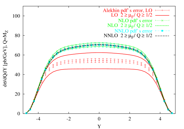
(a) Alekhin’s model

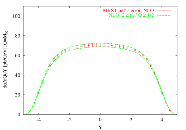
(b) MRST model

Figure 5.26: Plot of the rapidity distributions at LO, NLO and NNLO for Alekhin’s model and MRST. Shown are also the bands due to the variation of the $\mu_{F}$ scale, and the errors on the cross sections at the corresponding orders.

We have set the scales to be equal, $\mu_{F}=\mu_{R}$ and varied $\mu_{F}$ in the interval $1/2Q\leq\mu_{F}\leq 2Q$, obtaining results which differ from those obtained in [3] by $2\%$ due to the different implementation of the evolution. Using Candia and as initial condition the MRST grid input with $\mu_{0}^{2}=1.25$ GeV² the NNLO band and the NLO one are resolved separately. We have also found that with the inclusion of the $\mu_{R}^{2}/\mu_{F}^{2}$ effects in the pdf’s evolution, the dependence on $\mu_{R}$ is quite sizeable at NLO, but is reduced at NNLO [9]. We show in Fig. (5.26) the plots of the variations of the rapidity distributions at the three orders and the corresponding errors on the pdf’s for Alekhin’s model and for MRST for $Q=M_{Z}$. In both cases the reduction of the variation of the cross sections as we move toward higher orders is quite evident. We report also the errors on these distributions obtained in both models, which get systematically smaller as the accuracy of the calculation increases.

5.31 Conclusions

In the search for extra neutral currents precise theoretical determinations of lepton pair production via the Drell-Yan mechanism are going to play a very relevant role (see Ref. [14, 15, 16, 17, 18, 19]).

In our determination, the change in the value of the cross section from NLO to NNLO is around $4\%$ on the Z peak, while the MRST and the Alekhin determinations are $2.6\%$ and about $1.5\%$ respectively. While these variations appear to be more modest compared to the analogous ones at a lower order (which are of the order of $20\%$ or so), they are nevertheless important for the discovery of extra neutral currents at large invariant mass of the lepton pair in DY, given the fast falling cross section at those large values. The errors on the pdf’s induce percentile variations of the cross section as we move from NLO to NNLO of the order of $4\%$ around the best-fit result, reducing the NNLO cross section compared to the NLO prediction and rendering these results compatible.

Combination of QCD and electroweak corrections to Drell-Yan processes

G. Balossini, C.M. Carloni Calame, G. Montagna, M. Moretti, O. Nicrosini, F. Piccinini, M. Treccani and A. Vicini

Introduction

Precision measurements of electroweak (EW) gauge boson production and properties will be a crucial goal of the physics program of proton-proton collisions at the LHC. $W$ and $Z$ bosons will be produced copiously and careful measurements of their observables will be important in testing the Standard Model (SM) and uncovering signs of new physics [1, 2].

Thanks to the high luminosity achievable at the LHC, the systematic errors will play a dominant role in determining the accuracy of the measurements, implying, in particular, that the theoretical predictions will have to be of the highest standard as possible. For Drell-Yan (D-Y) processes, this amounts to make available calculations of $W$ and $Z$ production processes including simultaneously higher-order corrections coming from the EW and QCD sector of the SM. Actually, in spite of a detailed knowledge of EW and QCD corrections separately, the combination of their effects have been addressed only recently [3, 4, 5] and need to be deeply scrutinized in view of the anticipated experimental accuracy.

In this contribution, after a review of existing calculations and codes, we present the results of a study aiming at combining EW and QCD radiative corrections to D-Y processes consistently. We do not include in our analysis uncertainties due to factorization/renormalization scale variations, as well as uncertainties in the Parton Distribution Functions arising from diverse experimental and theoretical sources, which are left to a future publication. Some results already available in this direction can be found in [6].

Status of theoretical predictions and codes

Concerning QCD calculations and tools, the present situation reveals quite a rich structure, that includes next-to-leading-order (NLO) and next-to-next-to-leading-order (NNLO) corrections to $W/Z$ total production rate [7, 8], NLO calculations for $W,Z+1,2\,\,{\rm jets}$ signatures [9, 10] (available in the codes DYRAD and MCFM), resummation of leading and next-to-leading logarithms due to soft gluon radiation [11, 12] (implemented in the Monte Carlo ResBos), NLO corrections merged with QCD Parton Shower (PS) evolution (in the event generators MC@NLO [13] and POWHEG [14]), NNLO corrections to $W/Z$ production in fully differential form [15, 16] (available in the Monte Carlo program FEWZ), as well as leading-order multi-parton matrix elements generators matched with vetoed PS, such as, for instance, ALPGEN [17], MADEVENT [18], HELAC [19] and SHERPA [20].

As far as complete ${\cal O}(\alpha)$ EW corrections to D-Y processes are concerned, they have been computed independently by various authors in [21, 22, 23, 24, 25] for $W$ production and in [26, 27, 28, 29] for $Z$ production. Electroweak tools implementing exact NLO corrections to $W$ production are DK [21], WGRAD2 [22], SANC [24] and HORACE [25], while ZGRAD2 [26], HORACE [28] and SANC [29] include the full set of ${\cal O}(\alpha)$ EW corrections to $Z$ production. The predictions of a subset of such calculations have been compared, at the level of same input parameters and cuts, in the proceedings of the Les Houches 2005 [30] and TEV4LHC [31] workshops for $W$ production, finding a very satisfactory agreement between the various, independent calculations. A first set of tuned comparisons for the $Z$ production process has been recently performed and is available in [32].

From the calculations above, it turns out that NLO EW corrections are dominated, in the resonant region, by final-state QED radiation containing large collinear logarithms of the form $\log(\hat{s}/m_{l}^{2})$, where $\hat{s}$ is the squared partonic centre-of-mass (c.m.) energy and $m_{l}$ is the lepton mass. Since these corrections amount to several per cents around the jacobian peak of the $W$ transverse mass and lepton transverse momentum distributions and cause a significant shift (of the order of 100-200 MeV) in the extraction of the $W$ mass $M_{W}$ at the Tevatron, the contribution of higher-order corrections due to multiple photon radiation from the final-state leptons must be taken into account in the theoretical predictions, in view of the expected precision (at the level of 15-20 MeV) in the $M_{W}$ measurement at the LHC. The contribution due to multiple photon radiation has been computed, by means of a QED PS approach, in [33] for $W$ production and in [34] for $Z$ production, and implemented in the event generator HORACE. Higher-order QED contributions to $W$ production have been calculated independently in [35] using the YFS exponentiation, and are available in the generator WINHAC. They have been also computed in the collinear approximation, within the structure functions approach, in [36].

A further important phenomenological feature of EW corrections is that, in the region important for new physics searches (i.e. where the $W$ transverse mass is much larger than the $W$ mass or the invariant mass of the final state leptons is much larger than the $Z$ mass), the NLO EW effects become large (of the order of 20-30%) and negative, due to the appearance of EW Sudakov logarithms $\propto-(\alpha/\pi)\log^{2}({\hat{s}}/M_{V}^{2})$, $V=W,Z$ [21, 22, 25, 26, 27, 28]. Furthermore, in this region, weak boson emission processes (e.g. $pp\to e^{+}\nu_{e}V+X$), that contribute at the same order in perturbation theory, can partially cancel the large Sudakov corrections, when the weak boson $V$ decays into unobserved $\nu\bar{\nu}$ or jet pairs, as recently shown in [37].

Theoretical approach

A first strategy for the combination of EW and QCD corrections consists in the following formula

$$\left[\frac{d\sigma}{d\cal O}\right]_{{\rm QCD}\&{\rm EW}}=\left\{\frac{d\sigma}{d\cal O}\right\}_{{\rm MC@NLO}}+\left\{\left[\frac{d\sigma}{d\cal O}\right]_{{\rm EW}}-\left[\frac{d\sigma}{d\cal O}\right]_{{\rm Born}}\right\}_{{\rm HERWIG\,\,PS}}$$ (6.7)

where ${d\sigma/d\cal O}_{{\rm MC@NLO}}$ stands for the prediction of the observable ${d\sigma/d\cal O}$ as obtained by means of MC@NLO, ${d\sigma/d\cal O}_{{\rm EW}}$ is the HORACE prediction for the EW corrections to the ${d\sigma/d\cal O}$ observable, and ${d\sigma/d\cal O}_{{\rm Born}}$ is the lowest-order result for the observable of interest. The label HERWIG PS in the second term in r.h.s. of eq. (6.7) means that EW corrections are convoluted with QCD PS evolution through the HERWIG event generator, in order to (approximately) include mixed ${\cal O}(\alpha\alpha_{s})$ corrections and to obtain a more realistic description of the observables under study. However, it is worth noting that the convolution of NLO EW corrections with QCD PS implies that the contributions of the order of $\alpha\alpha_{s}$ are not reliable when hard non-collinear QCD radiation turns out to be relevant, e.g. for the lepton and vector boson transverse momentum distributions in the absence of severe cuts able to exclude resonant $W/Z$ production. In this case, a full ${\cal O}(\alpha\alpha_{s})$ calculation would be needed for a sound evaluation of mixed EW and QCD corrections. Full ${\cal O}(\alpha)$ EW corrections to the exclusive process $pp\to W+j$ (where $j$ stands for jet) have been recently computed, in the approximation of real $W$ bosons, in [38, 39], while one-loop weak corrections to $Z$ hadro-production have been computed, for on-shell $Z$ bosons, in [40]. It is also worth stressing that in eq. (6.7) the infrared part of QCD corrections is factorized, whereas the infrared-safe matrix element residue is included in an additive form. It is otherwise possible to implement a fully factorized combination (valid for infra-red safe observables) as follows:

$$\left[\frac{d\sigma}{d\cal O}\right]_{{\rm QCD}\otimes{\rm EW}}= \left(1+\frac{\left[{d\sigma}/{d\cal O}\right]_{\rm MC@NLO}-\left[{d\sigma}/{d\cal O}\right]_{\rm HERWIG\,\,PS}}{\left[{d\sigma}/{d\cal O}\right]_{\rm Born}}\right)\times$$ (6.8)

$$\times\left\{\frac{d\sigma}{{d\cal O}_{\rm EW}}\right\}_{{\rm HERWIG\,\,PS}},$$

where the ingredients are the same as in eq. (6.7) but also the QCD matrix element residue in now factorized. Eqs. (6.7) and  (6.8) have the very same ${\cal O}(\alpha)$ and ${\cal O}(\alpha_{s})$ content, differing by terms of the order of $\alpha\alpha_{s}$. Their relative difference has been checked to be of the order of a few per cent in the resonance region around the $W$/$Z$ mass, and can be taken as an estimate of the uncertainty of QCD and EW combination.

Numerical results: $W$ and $Z$ production

In order to assess the phenomenological relevance of the combination of QCD and EW corrections, we study, for definiteness, the charged-current process $pp\to W^{\pm}\to\mu^{\pm}+X$ at the LHC, imposing the following selection criteria

$${\rm a.}\quad p_{\perp}^{\mu}\geq~{}25~{}{\rm GeV},~{}~{}~{}~{}\hbox to0.0pt{/\hss}{\!E_{T}}\geq~{}25~{}{\rm GeV},~{}~{}~{}~{}|\eta_{\mu}|<2.5,$$

$${\rm b.}\quad{\rm the\,\,cuts\,\,as\,\,above}\,\,\oplus\,\,M_{\perp}^{W}\geq 1~{}{\rm TeV},$$ (6.9)

where $p_{\perp}^{\mu}$ and $\eta_{\mu}$ are the transverse momentum and the pseudorapidity of the muon, $\hbox to0.0pt{/\hss}{\!E_{T}}$ is the missing transverse energy, which we identify with the transverse momentum of the neutrino, as typically done in several phenomenological studies. For set up b., a severe cut on the $W$ transverse mass $M_{\perp}^{W}$ is superimposed to the cuts of set up a., in order to isolate the region of the high tail of $M_{T}^{W}$, which is interesting for new physics searches. We also consider the neutral-current reaction $pp\to\gamma,Z\to e^{+}e^{-}+X$, selecting the events according to the cuts

$$p_{\perp}^{e^{\pm}}\geq 25~{}{\rm GeV},~{}~{}~{}~{}|\eta^{e^{\pm}}|<2.5,~{}~{}~{}~{}M_{e^{+}e^{-}}\geq 200~{}{\rm GeV}.$$ (6.10)

The granularity of the detectors and the size of the electromagnetic showers in the calorimeter make it difficult to discriminate between electrons and photons with a small opening angle. We adopt the following procedure to select the event: we recombine the four-momentum vectors of the electron and photon into an effective electron four-momentum vector if, defining

$$\Delta R(e,\gamma)=\sqrt{\Delta\eta(e,\gamma)^{2}+\Delta\phi(e,\gamma)^{2}},$$ (6.11)

$\Delta R(e,\gamma)<0.1$ (with $\Delta\eta,\Delta\phi$ the distances of electrons and photons along the longitudinal and azimuthal directions). We do not recombine electrons and photons if $\eta_{\gamma}>2.5$ (with $\eta_{\gamma}$ the photon pseudo-rapidity). We apply the event selection cuts as in Eq. (6.10) only after the recombination procedure.

The parton distribution function (PDF) set MRST2004QED [41] has been used to describe the proton partonic content. The QCD factorization/renormalization scale and the analogous QED scale (present in the PDF set MRST2004QED) are chosen to be equal, as usually done in the literature [21, 22, 25, 26, 28], and fixed at $\mu_{R}=\mu_{F}=\sqrt{\left(p_{\perp}^{W}\right)^{2}+M_{\mu\nu_{\mu}}^{2}}$ (for the charged-current case), where $M_{\mu\nu_{\mu}}$ is the $\mu\nu_{\mu}$ invariant mass, and at $\mu_{R}=\mu_{F}=\sqrt{\left(p_{\perp}^{Z}\right)^{2}+M^{2}_{e^{+}e^{-}}}$ (for the neutral-current case), where $M_{e^{+}e^{-}}$ is the invariant mass of the lepton pair.

In order to avoid systematics theoretical effects, all the generators used in our study have been properly tuned at the level of input parameters, PDF set and scale to give the same LO/NLO results. The tuning procedure validates the interpretation of the various relative effects as due to the radiative corrections and not to a mismatch in the setups of the codes under consideration.

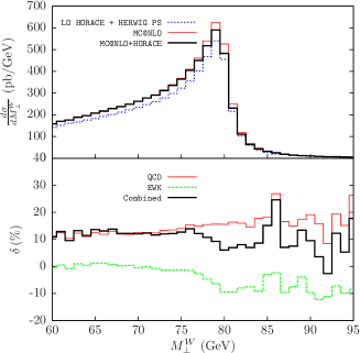
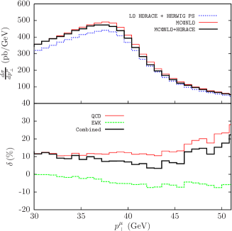
Figure 6.27: Upper panel: predictions of MC@NLO, MC@NLO+HORACE and leading-order HORACE+HERWIG PS for the $M_{\perp}^{W}$ (left) and $p_{\perp}^{\mu}$ (right) distributions at the LHC, according to the cuts of set up a. of Eq. (6.9). Lower panel: relative effect of QCD and EW corrections, and their sum, for the corresponding observables in the upper panel.

A sample of our numerical results is shown in Fig. 6.27 for the $W$ transverse mass $M_{\perp}^{W}$ and muon transverse momentum $p_{\perp}^{\mu}$ distributions according to set up a. of Eq. (6.9), and in Fig. 6.28 for the same distributions according to set up b. In Fig. 6.27 and Fig. 6.28, the upper panels show the predictions of the generators MC@NLO and MC@NLO + HORACE interfaced to HERWIG PS (according to eq. (6.7)), in comparison with the leading-order result by HORACE convoluted with HERWIG shower evolution. The lower panels illustrate the relative effects of the matrix element residue of NLO QCD and of full EW corrections, as well as their sum, that can be obtained by appropriate combinations of the results shown in the upper panels. More precisely, the percentage corrections shown have been defined as $\delta=\left(\sigma_{\rm NLO}-\sigma_{\rm Born+HERWIG\,PS}\right)/\sigma_{\rm Born+HERWIG\,PS}$, where $\sigma_{\rm NLO}$ stands for the predictions of the generators including exact NLO corrections matched with QCD PS.

From Fig. 6.27 it can be seen that the QCD corrections are positive around the $W$ jacobian peak, of about 10-20%, and tend to compensate the negative effect due to EW corrections. Therefore, their interplay is crucial for a precise $M_{W}$ extraction at the LHC and their combined contribution can not be accounted for in terms of a pure QCD PS approach, as it can be inferred from the comparison of the predictions of MC@NLO versus the leading-order result by HORACE convoluted with HERWIG PS. It is also worth noting that the convolution of NLO corrections with the QCD PS broadens the sharply peaked shape of the fixed-order NLO QCD and EW effects.

The interplay between QCD and EW corrections to $W$ production in the region interesting for new physics searches, i.e. in the high tail of $M_{\perp}^{W}$ and $p_{\perp}^{\mu}$ distributions, is shown in Fig. 6.28. For both $M_{\perp}^{W}$ and $p_{\perp}^{\mu}$, the QCD corrections are positive and largely cancel the negative EW Sudakov logarithms. Therefore, a precise normalization of the SM background to new physics searches necessarily requires the simultaneous control of QCD and EW corrections.

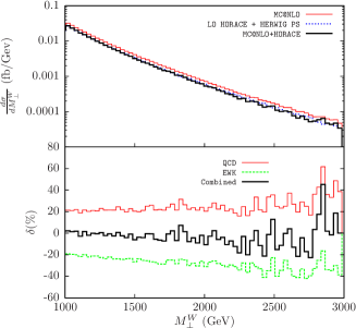
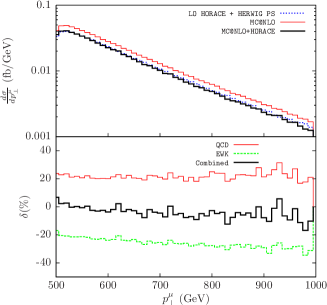
Figure 6.28: The same as Fig. 6.27 according to the cuts of set up b. of Eq. (6.9).

Figure 6.29 shows the combination of QCD and EW corrections for the di-lepton invariant mass in the neutral-current D-Y process $pp\to\gamma,Z\to e^{+}e^{-}+X$, according to the cuts of Eq. (6.10) [42]. The QCD corrections are quite flat and positive with a value of about $15\%$ over the mass range 200–1500 GeV. The EW corrections are negative and vary from about $-5\%$ to $-10\%$ and thus partially cancel the QCD contribution. Therefore, as for the charged-current channel, the search for new physics in di-lepton final states needs a careful combination of EW and QCD effects.

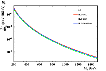
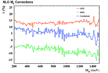
Figure 6.29: Left panel: the di-electron invariant mass distribution according to the leading-order and NLO EW predictions of HORACE, of MC@NLO and of MC@NLO+HORACE at the LHC, using the cuts of Eq. (6.10). Right panel: relative effect of QCD and EW corrections, and their combination.

Conclusions

During the last few years, there has been a big effort towards high-precision predictions for D-Y-like processes, addressing the calculation of higher-order QCD and EW corrections. Correspondingly, precision computational tools have been developed to keep under control theoretical systematics in view of the future measurements at the LHC.

We presented some original results about the combination of EW and QCD corrections to a sample of observables of $W$ and $Z$ production processes at the LHC. Our investigation shows that a high-precision knowledge of QCD and a careful combination of EW and strong contributions is mandatory in view of the anticipated experimental accuracy. We plan, however, to perform a more complete and detailed phenomenological study, including the predictions of other QCD generators and considering further observables of interest for the many facets of the $W/Z$ physics program at the LHC.

Acknowledgements

C.M. Carloni Calame is supported by a INFN postdoc Fellowship and thanks the School of Physics&Astronomy, University of Southampton, for hospitality. We acknowledge useful discussions with P. Nason and other participants of the workshop. We are also grateful to the colleagues of the common paper [42] for precious collaboration.

Subtraction at NNLO and Higgs boson production at hadron colliders

M. Grazzini

7.32 Introduction

The dynamics of hard scattering processes involving hadrons is nowadays remarkably well described by perturbative QCD predictions. Thanks to asymptotic freedom, the cross section for sufficiently inclusive reactions can be computed as a series expansion in the QCD coupling $\alpha_{\mathrm{S}}$. Until few years ago, the standard for such calculations was next-to-leading order (NLO) accuracy. Next-to-next-to-leading order (NNLO) results were known only for few highly-inclusive reactions (see e.g. Refs. [1, 2, 3]).

The extension from NLO to NNLO accuracy is important to improve QCD predictions and to better assess their uncertainties. In particular, this extension is essential in two cases: in those processes whose NLO corrections are comparable to the leading order (LO) contribution; in those ‘benchmark’ processes that are measured with high experimental precision. Such a task, however, implies finding methods and techniques to cancel the infrared (IR) divergences that appear at intermediate steps of the calculations.

Recently, a new general method [4], based on sector decomposition [5], has been proposed and applied to the NNLO QCD calculations of $e^{+}e^{-}\to 2~{}{\rm jets}$ [6], Higgs [7] and vector [8] boson production in hadron collisions, and to the NNLO QED calculation of the electron energy spectrum in muon decay [9]. The calculations of Refs. [7, 8] allow us to compute the corresponding cross sections with arbitrary cuts on the momenta of the partons produced in the final state.

The traditional approach to perform NLO computations is based on the introduction of auxiliary cross sections that are obtained by approximating the QCD scattering amplitudes in the relevant IR (soft and collinear) limits. This strategy led to the proposal of the subtraction [10] and slicing [11] methods. Exploiting the universality properties of soft and collinear emission, these methods were later developed in the form of general algorithms [12, 13, 14]. that make possible to perform NLO calculations in a (relatively) straightforward manner, once the corresponding QCD amplitudes are available. In recent years, several research groups have been working on general NNLO extensions of the subtraction method [15, 16, 17, 18, 19]. Results have been obtained in some specific processes: $e^{+}e^{-}\to 2~{}{\rm jets}$ [20, 21] and, more recently, $e^{+}e^{-}\to 3~{}{\rm jets}$ [22, 23].

In Ref. [24] we proposed an extension of the subtraction method to NNLO for a specific, though important, class of processes: the production of colourless high-mass systems in hadron collisions. We presented a formulation of the subtraction method for this class of processes, and we applied it to the NNLO calculation of Higgs boson production via the gluon fusion subprocess $gg\to H$. The calculation has now been implemented in the numerical program HNNLO, which includes all the relevant decay modes of the Higgs boson for this production subprocess, namely, $H\to\gamma\gamma$ [24], $H\to WW\to l\nu l\nu$ and $H\to ZZ\to 4l$ [25].

This contribution is organized as follows. In Sect. 7.33 we discuss the version of the subtraction formalism we use. In Sect. 7.34 we present a selection of numerical results that can be obtained by our program. In Sect. 7.35 we summarize our results.

7.33 The method

We consider the inclusive hard-scattering reaction

$$h_{1}+h_{2}\to F(Q)+X,$$ (7.12)

where the collision of the two hadrons $h_{1}$ and $h_{2}$ produces the triggered final state $F$. The final state $F$ consists of one or more colourless particles (leptons, photons, vector bosons, Higgs bosons, $\dots$) with momenta $q_{i}$ and total invariant mass $Q$ . Note that, since $F$ is colourless, the LO partonic subprocess is either $q{\bar{q}}$ annihilation, as in the case of the Drell–Yan process, or $gg$ fusion, as in the case of Higgs boson production.

At NLO, two kinds of corrections contribute: i) real corrections, where one parton recoils against $F$; ii) one-loop virtual corrections to the LO subprocess. Both contributions are separately IR divergent, but the divergences cancel in the sum. At NNLO, three kinds of corrections must be considered: i) double real contributions, where two partons recoil against $F$; ii) real-virtual corrections, where one parton recoils against $F$ at one-loop order; iii) two-loop virtual corrections to the LO subprocess. The three contributions are still separately divergent, and the calculation has to be organized so as to explicitly achieve the cancellation of the IR divergences.

Our method is based on a generalization of the procedure used in the specific NNLO calculation of Ref. [26]. We first note that, at LO, the transverse momentum ${\bf q}_{\,T}$ of the triggered final state $F$ is exactly zero. As a consequence, as long as $q_{T}\neq 0$, the (N)NLO contributions are actually given by the (N)LO contributions to the triggered final state $F+{\rm jet(s)}$. Thus, we can write the cross section as

$$d{\sigma}^{F}_{(N)NLO}|_{q_{T}\neq 0}=d{\sigma}^{F+{\rm jets}}_{(N)LO}\;\;.$$ (7.13)

This means that, when $q_{T}\neq 0$, the IR divergences in our NNLO calculation are those in $d{\sigma}^{F+{\rm jets}}_{NLO}$: they can be handled and cancelled by using available NLO formulations of the subtraction method. The only remaining singularities of NNLO type are associated to the limit $q_{T}\to 0$, and we treat them by an additional subtraction. Our key point is that the singular behaviour of $d{\sigma}^{F+{\rm jets}}_{(N)LO}$ when $q_{T}\to 0$ is well known: it appears in the resummation program [27, 28, 29] of logarithmically-enhanced contributions to transverse-momentum distributions. Then, to perform the additional subtraction, we follow the formalism used in Ref. [30, 31] to combine resummed and fixed-order calculations.

We use a shorthand notation that mimics the notation of Ref. [30]. We define the subtraction counterterm

$$d{\sigma}^{CT}=d{\sigma}_{LO}^{F}\otimes\Sigma^{F}(q_{T}/Q)\,d^{2}{\bf q}_{\,T}.$$ (7.14)

The function $\Sigma^{F}(q_{T}/Q)$ embodies the singular behaviour of $d{\sigma}^{F+{\rm jets}}$ when $q_{T}\to 0$. In this limit it can be expressed as follows in terms of $q_{T}$-independent coefficients $\Sigma^{F(n;k)}$:

$$\Sigma^{F}(q_{T}/Q)\xrightarrow[q_{T}\to 0]{}\sum_{n=1}^{\infty}\left(\frac{\alpha_{\mathrm{S}}}{\pi}\right)^{n}\sum_{k=1}^{2n}\Sigma^{F(n;k)}\;\frac{Q^{2}}{q_{T}^{2}}\ln^{k-1}\frac{Q^{2}}{q_{T}^{2}}\;\;.$$ (7.15)

The extension of Eq. (7.13) to include the contribution at $q_{T}=0$ is finally:

$$d{\sigma}^{F}_{(N)NLO}={\cal H}^{F}_{(N)NLO}\otimes d{\sigma}^{F}_{LO}+\left[d{\sigma}^{F+{\rm jets}}_{(N)LO}-d{\sigma}^{CT}_{(N)LO}\right]\;\;.$$ (7.16)

Comparing with the right-hand side of Eq. (7.13), we have subtracted the truncation of Eq. (7.14) at (N)LO and added a contribution at $q_{T}=0$ needed to obtain the correct total cross section. The coefficient ${\cal H}^{F}_{(N)NLO}$ does not depend on $q_{T}$ and is obtained by the (N)NLO truncation of the perturbative function

$${\cal H}^{F}=1+\frac{\alpha_{\mathrm{S}}}{\pi}\,{\cal H}^{F(1)}+\left(\frac{\alpha_{\mathrm{S}}}{\pi}\right)^{2}{\cal H}^{F(2)}+\dots\;\;.$$ (7.17)

The counterterm of Eq. (7.14) regularizes the singularity of $d{\sigma}^{F+{\rm jets}}$ when $q_{T}\to 0$: the term in the square bracket on the right-hand side of Eq. (7.16) is thus IR finite (or, better, integrable over $q_{T}$). Note that, at NNLO, $d{\sigma}^{CT}_{(N)LO}$ acts as a counterterm for the sum of the two contributions to $d{\sigma}^{F+{\rm jets}}$: the double real plus real-virtual contributions. We also note that the counterterm function $\Sigma^{F}(q_{T}/Q)$ can be defined in different ways: the only property we require is that in the small $q_{T}$ limit it must take the form given in Eq. (7.15), so as to match the singular behaviour of $d{\sigma}^{F+{\rm jets}}$. Note that the perturbative coefficients $\Sigma^{F(n;k)}$ are universal: more precisely, the NNLO coefficients $\Sigma^{F(2;1)}$ and $\Sigma^{F(2;2)}$ have a non-universal contribution that, nonetheless, is proportional to the NLO coefficient ${\cal H}^{F(1)}$. The above coefficients only depend on the type of partons (quarks or gluon) involved in the LO partonic subprocess ($q{\bar{q}}$ annihilation or $gg$ fusion). We finally note that the simplicity of the LO subprocess is such that final-state partons actually appear only in the term $d{\sigma}^{F+{\rm jets}}$ on the right-hand side of Eq. (7.16). Therefore, arbitrary IR-safe cuts on the jets at (N)NLO can effectively be accounted for through a (N)LO computation. Owing to this feature, our NNLO extension of the subtraction formalism is observable-independent.

At NLO (NNLO), the physical information of the one-loop (two-loop) virtual correction to the LO subprocess is contained in the coefficients ${\cal H}^{(1)}$ (${\cal H}^{(2)}$). Once an explicit form of Eq. (7.14) is chosen, the hard coefficients ${\cal H}^{F(n)}$ are uniquely identified (a different choice would correspond to different ${\cal H}^{F(n)}$). According to Eq. (7.16), the NLO calculation of $d{\sigma}^{F}$ requires the knowledge of ${\cal H}^{F(1)}$ and the LO calculation of $d{\sigma}^{F+{\rm jets}}$. The general (process-independent) form of the coefficient ${\cal H}^{F(1)}$ is basically known: the precise relation between ${\cal H}^{F(1)}$ and the IR finite part of the one-loop correction to a generic LO subprocess is explicitly derived in Ref. [32].

At NNLO, the coefficient ${\cal H}^{F(2)}$ is also needed, together with the NLO calculation of $d{\sigma}^{F+{\rm jets}}$. The coefficients ${\cal H}^{H(2)}$ for Higgs boson production in the large-$M_{top}$ limit have been computed [33]. Since the NLO corrections to $gg\to H+{\rm jet(s)}$ are available [34] in the same limit, we are able to apply Eq. (7.16) at NNLO. We have encoded our computation in a parton level Monte Carlo program, in which we can implement arbitrary IR-safe cuts on the final state.

7.34 Results

In the following we present numerical results for Higgs boson production at the LHC. We use the MRST2004 parton distributions [35], with densities and $\alpha_{\mathrm{S}}$ evaluated at each corresponding order (i.e., we use $(n+1)$-loop $\alpha_{\mathrm{S}}$ at NⁿLO, with $n=0,1,2$). The renormalization and factorization scales are fixed to the value $\mu_{R}=\mu_{F}=M_{H}$, where $M_{H}$ is the mass of the Higgs boson.

7.34.1 $H\to\gamma\gamma$

We consider the Higgs boson decay in the $H\to\gamma\gamma$ channel and follow Ref. [36] to apply cuts on the photons. For each event, we classify the photon transverse momenta according to their minimum and maximum value, $p_{T{\rm min}}$ and $p_{T{\rm max}}$. The photons are required to be in the central rapidity region, $|\eta|<2.5$, with $p_{T{\rm min}}>35$ GeV and $p_{T{\rm max}}>40$ GeV. We also require the photons to be isolated: the hadronic (partonic) transverse energy in a cone of radius $R=0.3$ along the photon direction has to be smaller than 6 GeV. When $M_{H}=125$ GeV, by applying these cuts the impact of the NNLO corrections on the NLO total cross section is reduced from 19% to 11%.

Figure 7.30: Distributions in $p_{T{\rm min}}$ and $p_{T{\rm max}}$ for the diphoton signal at the LHC. The cross section is divided by the branching ratio in two photons.

In Fig. 7.30 we plot the distributions in $p_{T{\rm min}}$ and $p_{T{\rm max}}$ for the $gg\to H\to\gamma\gamma$ signal. We note that the shape of these distributions sizeably differs when going from LO to NLO and to NNLO. The origin of these perturbative instabilities is well known [37]. Since the LO spectra are kinematically bounded by $p_{T}\leq M_{H}/2$, each higher-order perturbative contribution produces (integrable) logarithmic singularities in the vicinity of that boundary. More detailed studies are necessary to assess the theoretical uncertainties of these fixed-order results and the relevance of all-order resummed calculations.

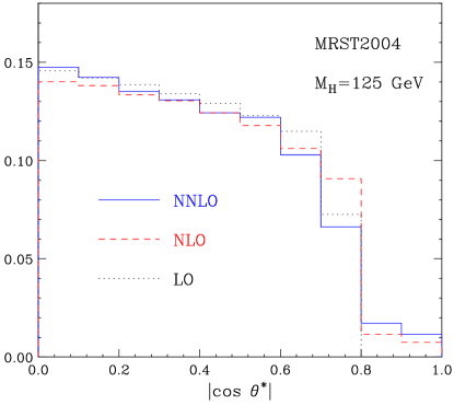
Figure 7.31: Normalized distribution in the variable $\cos\theta^{*}$.

In Fig. 7.31 we consider the (normalized) distribution in the variable $\cos\theta^{*}$, where $\theta^{*}$ is the polar angle of one of the photons in the rest frame of the Higgs boson. At small values of $\cos\theta^{*}$ the distribution is quite stable with respect to higher order QCD corrections. We also note that the LO distribution vanishes beyond the value $\cos\theta^{*}_{\rm max}<1$. The upper bound $\cos\theta^{*}_{\rm max}$ is due to the fact that the photons are required to have a minimum $p_{T}$ of $35$ GeV. As in the case of Fig. 7.30, in the vicinity of this LO kinematical boundary there is an instability of the perturbative results beyond LO.

7.34.2 $H\to WW\to l\nu l\nu$

We now consider the production of a Higgs boson with mass $M_{H}=165$ GeV in the decay mode $H\to WW\to l\nu l\nu$ [25]. We apply a set of selection cuts taken from the study of Ref. [38]. The charged leptons are classified according to their minimum and maximum $p_{T}$. The $p_{T{\rm min}}$ should be larger than 25 GeV, and $p_{T{\rm max}}$ should be between 35 and 50 GeV. The charged lepton rapidity should fullfil $|\eta|<2$. The missing $p_{T}$ of the event is required to be larger than $20$ GeV and the invariant mass of the charged leptons is smaller than $35$ GeV. The azimuthal separation of the charged leptons in the transverse plane ($\Delta\phi$) is smaller than $45^{o}$. Finally, there should be no jet with $p_{T}^{\rm jet}$ larger than $p_{T}^{\rm veto}$ .

In Table 7.9 we report the corresponding cross sections in the case of $p_{T}^{\rm veto}=30$ GeV.

$\sigma$ (fb)	LO	NLO	NNLO
$\mu_{F}=\mu_{R}=M_{H}/2$	$17.36\pm 0.02$	$18.11\pm 0.08$	$15.70\pm 0.32$
$\mu_{F}=\mu_{R}=M_{H}$	$14.39\pm 0.02$	$17.07\pm 0.06$	$15.99\pm 0.23$
$\mu_{F}=\mu_{R}=2M_{H}$	$12.00\pm 0.02$	$15.94\pm 0.05$	$15.68\pm 0.20$

Table 7.9: Cross sections for $pp\to H+X\to WW+X\to l\nu l\nu+X$ at the LHC when selection cuts are applied and $p_{T}^{\rm veto}=30$ GeV.

The cuts are quite hard, the efficiency being $8\%$ at NLO and $6\%$ at NNLO. The scale dependence of the result is strongly reduced at NNLO, being of the order of the error from the numerical integration. The impact of higher order corrections is also drastically changed. The $K$-factor is now 1.19 at NLO and 1.11 at NNLO. As expected, the jet veto tends to stabilize the perturbative expansion, and the NNLO cross section turns out to be smaller than the NLO one.

7.34.3 $H\to ZZ\to e^{+}e^{-}e^{+}e^{-}$

We now consider the production of a Higgs boson with mass $M_{H}=200$ GeV [25]. In this mass region the dominant decay mode is $H\to ZZ\to 4$ leptons, providing a clean four lepton signature. In the following we consider the decay of the Higgs boson in two identical lepton pairs. When no cuts are applied, the NLO $K$-factor is $K=1.87$ whereas at NNLO we have $K=2.26$. We find that the interference contribution is smaller than $1\%$ in this region of Higgs boson masses.

We consider the following cuts [36]:

1. For each event, we order the transverse momenta of the leptons from the largest ($p_{T1}$) to the smallest ($p_{T4}$). They are required to fulfil the following thresholds:
   $p_{T1}>30~{}{\rm GeV}~{}~{}~{}~{}p_{T2}>25~{}{\rm GeV}~{}~{}~{}~{}p_{T3}>15~{}{\rm GeV}~{}~{}~{}~{}p_{T4}>7~{}{\rm GeV}$ ;

2. Leptons should be central: $|y|<2.5$;

3. Leptons should be isolated: the total transverse energy $E_{T}$ in a cone of radius 0.2 around each lepton should fulfil $E_{T}<0.05~{}p_{T}$;

4. For each possible $e^{+}e^{-}$ pair, the closest ($m_{1}$) and next-to-closest ($m_{2}$) to $M_{Z}$ are found. Then $m_{1}$ and $m_{2}$ are required to be $81$ GeV $<m_{1}<101$ GeV and $40$ GeV $<m_{2}<110$ GeV.

These cuts are designed to maximize the statistical significance for an early discovery, but to keep the possibility for a more detailed analysis of the properties of the Higgs boson. The corresponding cross sections are reported in Table 7.10.

$\sigma$ (fb)	LO	NLO	NNLO
$\mu_{F}=\mu_{R}=M_{H}/2$	$1.541\pm 0.002$	$2.764\pm 0.005$	$3.013\pm 0.023$
$\mu_{F}=\mu_{R}=M_{H}$	$1.264\pm 0.001$	$2.360\pm 0.003$	$2.805\pm 0.015$
$\mu_{F}=\mu_{R}=2M_{H}$	$1.047\pm 0.001$	$2.044\pm 0.003$	$2.585\pm 0.010$

Table 7.10: Cross sections for $pp\to H+X\to ZZ+X\to e^{+}e^{-}e^{+}e^{-}+X$ at the LHC when cuts are applied.

Contrary to what happens in the $H\to WW\to l\nu l\nu$ decay mode, the cuts are quite mild, the efficiency being $63\%$ at NLO and $62\%$ at NNLO. The NLO and NNLO $K$-factors are $1.87$ and $2.22$, respectively. Comparing with the inclusive case, we conclude that these cuts do not change significantly the impact of QCD radiative corrections. We also find that the effect of lepton isolation is mild: at NNLO it reduces the accepted cross section by about $4\%$.

Figure 7.32: Tranverse momentum spectra of the final state leptons for $pp\to H+X\to ZZ+X\to e^{+}e^{-}e^{+}e^{-}+X$, ordered according to decreasing $p_{T}$, at LO (dotted), NLO (dashed), NNLO (solid).

In Fig. 7.32 we report the $p_{T}$ spectra of the charged leptons. We note that at LO, without cuts, the $p_{T1}$ and $p_{T2}$ are kinematically bounded by $M_{H}/2$, whereas $p_{T3}<M_{H}/3$ and $p_{T4}<M_{H}/4$. Contrary to what happens in the $H\to\gamma\gamma$ decay mode (see Sect. 7.34.1) the distributions smoothly reach the kinematical boundary, and no perturbative instability is observed beyond LO.

7.35 Summary

We have illustrated an extension of the subtraction formalism to compute NNLO QCD corrections to the production of high-mass systems in hadron collisions. We have considered an explicit application of our method to the NNLO computation of $gg\to H$ at the LHC, including the decay of the Higgs boson in all the relevant decay modes, namely, $H\to\gamma\gamma$, $H\to WW\to l\nu l\nu$ and $H\to ZZ\to 4$ leptons. We have presented few selected results, including kinematical cuts on the final state. In the case of the $H\to\gamma\gamma$ and $H\to WW\to l\nu l\nu$ decay modes, our computation parallels the one of Refs. [7, 40], but it is performed with a completely independent method. In the quantitative studies that we have carried out, the two computations give results in numerical agreement. In our approach the calculation is directly implemented in a parton level event generator. This feature makes it particularly suitable for practical applications to the computation of distributions in the form of bin histograms. The calculation is implemented in the numerical program HNNLO, which can be downloaded from [41].

QCD final states: resummation and Monte Carlo simulations

A. Banfi

8.36 Introduction

Any short distance dominated cross section $d\sigma$ in QCD can be written as a formal series in the QCD coupling $\alpha_{s}$:

$$d\sigma=d\sigma_{0}+\alpha_{s}\cdot d\sigma_{1}+\alpha_{s}^{2}\cdot d\sigma_{2}+\dots$$ (8.18)

where $d\sigma_{0}$ is the leading order (LO) or Born contribution, $d\sigma_{1}$ the next-to-leading order (NLO) contribution, $d\sigma_{2}$ the next-to-next-to-leading order (NNLO) and so on. In spite of the smallness of $\alpha_{s}$, the coefficients of the expansion may be large. This happens typically when a process is characterised by two widely separated scales $Q$ and $Q_{0}$, where $Q$ represents the hard scale of the process and $Q_{0}$ an energy resolution. In this case large logarithms $L=\ln Q/Q_{0}$ arise at any order in the perturbative (PT) series eq. (8.18), and only after an all-order resummation can one give meaning to the PT expansion. In many cases resummation makes it possible to rewrite $d\sigma$ as an exponent

$$d\sigma=C(\alpha_{s})\exp\left(Lg_{1}(\alpha_{s}L)+g_{2}(\alpha_{s}L)+\alpha_{s}g_{3}(\alpha_{s}L)\right)+\mbox{suppressed terms}\>,$$ (8.19)

where $g_{1}$ resums the leading logarithms (LL, $\alpha_{s}^{n}L^{n+1}$), $g_{2}$ the next-to-leading logarithms (NLL, $\alpha_{s}^{n}L^{n}$), $g_{3}$ the next-to-next-to-leading logarithms (NNLL, $\alpha_{s}^{n}L^{n-1}$), and so on.

The physical origin of large logarithms is the incomplete cancellation of soft and collinear (SC) singularities between real and virtual contributions. In particular we distinguish between double logarithms $\alpha_{s}L^{2}$ arising from soft and collinear emissions, and single logarithms $\alpha_{s}L$ from hard collinear or soft large-angle emissions. SC singularities factorise [1] from hard matrix elements and build up the exponent in eq. (8.19). Finite virtual corrections and the exact treatment of the phase space in the SC limit give the multiplicative constant $C(\alpha_{s})$, while hard emission contributions are suppressed by powers of $Q_{0}/Q$.

The above discussion can be visualised with the help of Lund diagrams. Consider for instance the well-known example of vector or Higgs boson production in hadron-hadron collisions. A generic contribution to the total cross section for this process in the SC limit is illustrated in fig. 8.33. Each dot represents an emitted parton, identified via its rapidity ($\eta$, on the $x$ axis) and transverse momentum ($\ln k_{t}/Q$, on the $y$ axis) with respect to the beam. The hard vertex is the origin of the axes. The yellow bands represent the collinear limit $\eta<\ln(2E_{\ell}/k_{t})$, where $E_{\ell}$ is the energy of emitting hard parton (leg) $\ell=1,2$. Hard collinear emissions (blue) are kinks on the two bands, since they reduce the emitting parton energy by a significant fraction. Soft large-angle emissions (red) are along the line $\eta=0$, while all remaining black dots are soft and collinear emissions. Since for fixed $\alpha_{s}$ emissions are distributed uniformly in $\ln k_{t}/Q$ and $\eta$, an area in the picture corresponds to a double logarithmic contribution, a line to a single logarithm, while points represent ${\cal O}(\alpha_{s})$ corrections.

Virtual corrections are universal and can be shown to exponentiate [2]. The contribution of real emissions is instead observable dependent and can be represented as a vetoed region, where real emissions are forbidden, and only virtual contributions survive. According to the way the veto condition is imposed one can distinguish between

1. inclusive observables: no hadrons are directly observed, QCD radiation is restricted via energy-momentum conservation. In this case, after an integral transform, real contributions exponentiate to all (logarithmic) orders. An example of an inclusive observable is the cross section for the production of a non-QCD particle, for instance a Higgs boson [3];

2. final-state observables: one measures final-state hadron momenta, a typical example being event shape distributions and jet rates. In this case there is no general statement concerning the level of accuracy at which exponentiation holds.

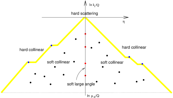
Figure 8.33: The Lund diagram for a generic contribution to the total cross section for the production of a vector or Higgs boson at hadronic colliders. Here $\mu_{0}$ is an infrared cut-off and the hard scale $Q$ is the boson mass.

Inclusive observables have been discussed during the workshop by Massimiliano Grazzini. Here I will concentrate on final-state observables, introducing specific classes of observables and discussing to what extent a resummation for those observables is feasible.

8.37 Global observables

Let us consider a global variable that measures hadrons everywhere, for instance the thrust in $e^{+}e^{-}$ annihilation, defined as

$$T=\max_{\vec{n}}\frac{\sum_{i}|\vec{p}_{i}\cdot\vec{n}|}{\sum_{i}|\vec{p}_{i}|}\>.$$ (8.20)

The thrust, as all other event shapes, is a measure of the geometrical properties of hadron energy-momentum flow. For instance, for pencil-like events we have $T\!\simeq\!1$, for planar events $T\!\simeq\!2/3$, while for spherical events $T\!\simeq\!1/2$. This variable has the property of infrared and collinear (IRC) safety, i.e. its value does not change after emission of extremely soft particles and/or quasi-collinear splittings. IRC safety is precisely the condition that ensures that observables related to the thrust, i.e. distributions and mean values, can be computed using the quark-gluon language, in spite of the fact that the variable definition involves hadrons, and the difference between parton and hadron level predictions is suppressed by powers of the hard scale $Q$.

The basic quantity we are interested in is $\Sigma(\tau)$, the probability that $1\!-\!T\!<\!\tau$, the differential distribution $\sigma^{-1}d\sigma/d\tau$ being the derivative of $\Sigma(\tau)$. Fixed order QCD predictions are reliable as long as $\tau$ is large, but fail as soon as events approach the Born limit $\tau\!=\!0$. In the small $\tau$ region one needs to resum logarithmic enhanced contributions to all orders, and the resulting resummed distribution has the same shape as the data. However, to get on top of the data, one needs to add a further correction that can be interpreted as the difference between parton and hadron level. This hadronisation correction can be estimated using Monte Carlo (MC) event generators like herwig [4], pythia [5, 6] or ariadne [7], taking the ratio of the distributions obtained with MC’s before and after hadronisation, and estimating hadronisation uncertainties using different event generators. This has lead to a successful description of IRC safe event shape distributions and jet rates in $e^{+}e^{-}$ annihilation, giving one of the most accurate measurements of $\alpha_{s}$ (see [8] for a recent review). The validity of this procedure relies strongly on the fact that MC event generators contain the physics that is needed to describe the main features of final-state observables. This statement is in general true for variables whose LL exponentiate, as we shall see in the following.

Consider then a generic final-state variable $V(\{k_{i}\})$, a function of final-state momenta $\{k_{i}\}$, and its rate $\Sigma(v)$, the probability that $V(\{k_{i}\})\!<\!v$. A generic contribution to $\Sigma(v)$ can be represented by the Lund diagram on the left hand side of fig. 8.34. The grey area corresponds to the vetoed region where no real emissions are allowed, and only virtual corrections survive, and one can write in general:

$$\Sigma(v)=e^{-R(v)}{\cal F}(v)\>,$$ (8.21)

where $R(v)$ is the exponent representing virtual corrections up to the scale $vQ$, while real emission outside the vetoed region and the remaining virtual corrections build up the function ${\cal F}(v)$. The variable $V$ is said to exponentiate if all leading (double) logarithms are contained in the exponent $R(v)$ and ${\cal F}(v)$ is a pure NLL function, usually denoted by ${\cal F}(R^{\prime})$, with $R^{\prime}(v)=-vdR/dv$. There are two basic conditions for this to happen, which go under the name of recursive infrared and collinear (rIRC) safety conditions [9]:

1. the variable must scale in the same fashion with multiple emissions as with a single emission. Formally, parametrising the momentum $k_{i}$ of each emission in terms of $V(k_{i})$, the value the variable $V$ would have if only emission $k_{i}$ were present, and defining $V(k_{i})=\bar{v}\zeta_{i}$, the first rIRC safety condition states that the following limit:

   $$\lim_{\bar{v}\to 0}\frac{V(k_{1}(\bar{v}\zeta_{1}),\dots,k_{n}(\bar{v}\zeta_{n}))}{\bar{v}}$$ (8.22)

   has to be finite and non-zero. This ensures that the boundary of the vetoed region in fig. 8.34 does not change substantially whatever is the number of emissions;

2. the variable’s scaling property (8.22) must not be altered by the addition of extra-soft particles or by quasi-collinear splittings, formally:

   $$[\lim_{\zeta_{n+1}\to 0},\lim_{\bar{v}\to 0}]\frac{V(k_{1}(\bar{v}\zeta_{1}),\dots,k_{n}(\bar{v}\zeta_{n}),k_{n+1}(\bar{v}\zeta_{n+1}))}{\bar{v}}=0\>,$$ (8.23)

   where the only non-trivial part of the commutator is the one where one takes the limit $\zeta_{n+1}\!\to\!0$ after the limit $\bar{v}\!\to\!0$, the other part being equal to the limit in eq. (8.22) due to IRC safety. An analogous condition should hold also for collinear splittings. This implies that in fig. 8.34 one can eliminate all emissions in grey, far from the boundary of the vetoed region, without altering the value of $V$, and for all emissions with $V(k_{i})\sim V(k_{1},\ldots,k_{n})$ one can replace clusters of emissions close in rapidity with a single emission having the total momentum of the cluster.

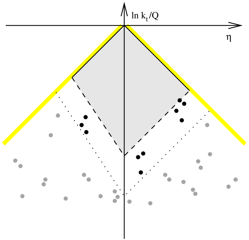
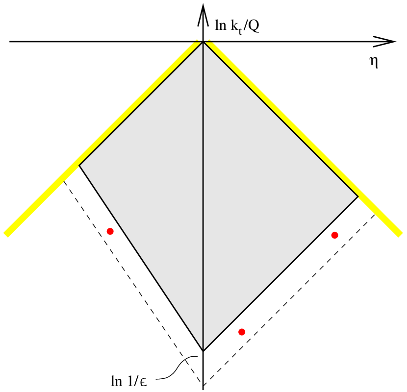
Figure 8.34: The Lund diagram for emissions contributing to a generic final-state observable (left) and its simplified version in case of a rIRC safe observable (right).

In the end, for a rIRC safe variable, a generic contribution to $\Sigma(v)$ can be represented by a Lund diagram like the one on the right hand side of fig. 8.34, where one has a vetoed area, giving rise to the LL exponent $R(v)$, and real emissions contributing to ${\cal F}(R^{\prime})$ at NLL accuracy are both soft and collinear, well separated in rapidity and confined in a narrow region of width $\ln 1/\epsilon\ll\ln 1/v$ close to the boundary of the vetoed area. The fact that emissions are well separated in rapidity makes it possible to exploit QCD coherence, and consider soft gluons as radiated independently (like in QED) from the hard legs. This simplification of multi-gluon soft matrix elements makes it possible to compute ${\cal F}(R^{\prime})$ with a MC procedure, where emissions are ordered in $V(k_{i})=\bar{v}\zeta_{i}$, with $\zeta_{i}<\zeta_{i-1}$, $V(k_{1})$ is fixed at $\bar{v}$, and the probability of emission of gluon $k_{i}$ collinear to leg $\ell$ with rapidity $\eta_{i}$ and azimuth $\phi_{i}$ (with respect to leg $\ell$) is

$$dP(k_{i}(\zeta_{i},\eta_{i},\phi_{i},\ell))=R^{\prime}_{\ell}\>\frac{d\eta_{i}}{\Delta\eta_{i}}\>\frac{d\phi_{i}}{2\pi}\>\frac{d\zeta_{i}}{\zeta_{i}}\left(\frac{\zeta_{i}}{\zeta_{i-1}}\right)^{R^{\prime}}\,,\qquad\sum_{\ell}R^{\prime}_{\ell}=R^{\prime}.$$ (8.24)

The function ${\cal F}(R^{\prime})$ can then be computed as the following average:

$${\cal F}(R^{\prime})=\left\langle\lim_{\bar{v}\to 0}\left(\frac{V(k_{1},\ldots,k_{n})}{V(k_{1})}\right)^{-R^{\prime}}\right\rangle\>,$$ (8.25)

where the limit $\bar{v}\to 0$ ensures that the result contains no NNLL contributions. Eq. (8.25) is an example of application of MC techniques used in parton shower event generators to obtain exact QCD results, and is one of the building blocks of the automated resummation program caesar [9].

We can now discuss what level of accuracy can be achieved by parton shower event generators. MC parton showers produce emissions in the whole of the phase space (for instance all emissions in the diagram on the left hand side of fig. 8.34), with approximated matrix elements that are exact in the collinear limit but mistreat the soft large-angle region, both because they do not have full interference terms, and because they are correct only in the large-$N_{c}$ limit. However, for rIRC safe observables, LL and NLL contributions are determined only by emissions that are well separated in rapidity and close to the boundary of the vetoed region. MC event generators correctly describe such emissions, so that one expects that they reproduce not only LL, but most NLL contributions to rIRC safe observables.

8.38 Non-global observables

Non-global variables measure hadrons in a restricted part of the phase space. The most relevant example is the hadron transverse energy flow in a region $\Omega$ away from the hard jets, defined as [10]

$$E_{t}=\sum_{i\in\Omega}E_{ti}\>,\qquad\Sigma(Q_{\Omega})=\int_{0}^{Q_{\Omega}}\!\!\!dE_{t}\frac{1}{\sigma}\frac{d\sigma}{dE_{t}}\>.$$ (8.26)

The distribution $\Sigma(Q_{\Omega})$ is sensitive only to soft emissions at large angles, so that LL are single logarithms $\alpha_{s}^{n}L^{n}$, with $L=\ln Q/Q_{\Omega}$. To achieve a LL resummation for $\Sigma(Q_{\Omega})$ one cannot rely on an independent emission picture of QCD radiation, because configurations like the one in fig. 8.35, where one has two emissions close in rapidity and the $k_{t}$ of the harder emission can take any value from $Q$ to $Q_{\Omega}$, give a single logarithm [10].

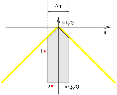
Figure 8.35: A configuration giving rise to non-global logarithms. The region $\Omega$ corresponds to a rapidity gap of width $\Delta\eta$ between the jets.

These non-global logarithms are ruled by the correlated part of soft gluon emission matrix elements, and can be resummed only in the large-$N_{c}$ limit. Furthermore, due to the fact that one needs to take into account the exact form of $\Omega$ for an arbitrary number of emissions, resummation can be performed only numerically. In the MC procedure of ref. [10], emissions are ordered in the variable $t=\int_{k_{t}}^{Q}\frac{dk}{k}\frac{\alpha_{s}(k)}{2\pi}\sim\alpha_{s}\ln Q/k_{t}$, with $t_{i}>t_{i-1}$, and, given an ensemble of $n\!-\!1$ colour connected soft gluons forming $n$ dipoles, a softer gluon $k_{i}$ is emitted from dipole $j$ with probability:

$$dP(k_{i}(t_{i},\eta_{i},\phi_{i},j))=2C_{A}d\eta_{i}\>\Theta\left(\frac{\Delta\eta_{j}}{2}-|\eta_{i}|\right)\>\frac{d\phi_{i}}{2\pi}\>dt_{i}\>e^{-2C_{A}\Delta\eta_{\mathrm{tot}}(t_{i}-t_{i-1})}\>,$$ (8.27)

where $\eta_{i}$ and $\phi_{i}$ are the rapidity and azimuth of emission $k_{i}$ in the frame in which partons forming dipole $j$ are back-to-back, $\Delta\eta_{j}$ represents a collinear cutoff and $\Delta\eta_{\mathrm{tot}}\!=\!\sum_{j}\Delta\eta_{j}$. The MC starts from a quark-antiquark dipole, and continues emitting gluons as long as one emission falls into $\Omega$. If one bins the value of $t$ corresponding to this last emission, when the MC stops one has reconstructed $d\Sigma(t)/dt$ at LL accuracy, with $t\!\sim\!\alpha_{s}\ln Q/Q_{\Omega}$.

Given the fact that the away-from-jet $E_{t}$ flow is used to tune MC models of the underlying event in hadron-hadron collisions, it is crucial to understand whether MC parton shower generators are able to describe $\Sigma(Q_{\Omega})$. If this is not the case, missing PT contributions, which are non-universal, will be included by tuning hadronisation and underlying event parameters, which are supposed to be universal. In ref. [11] it was first investigated the difference between a full treatment of soft radiation as in eq. (8.27), and an angular ordering (AO) approximation resulting from a free azimuthal average of $dP(k_{i})$ (see  [11] for details). The difference between the full and the AO distributions was found to be less than 10% in the whole range of values of $t$ relevant for phenomenology ($t\!<\!0.15$, corresponding to $Q_{\Omega}\!>\!1$GeV at the LEP1 energy), thus supporting the idea that MC generators implementing angular ordering should be able to give a reasonable description of $\Sigma(Q_{\Omega})$. Then a direct comparison of a LL resummation for $\sigma^{-1}d\sigma/dE_{t}$ in $e^{+}e^{-}$ annihilation and the corresponding predictions obtained with herwig and pythia at parton level was performed, the away-from-jet region $\Omega$ being a rapidity gap of width $\Delta\eta$ between the two jets. The comparison showed that herwig, whose evolution variable is the angle of each branching, is in good agreement with the LL resummation, discrepancies being less than 10%, both for large and small gaps. On the contrary, the old pythia shower [5], which uses the virtuality as an evolution variable and rejects a posteriori configurations not respecting AO, lies below the resummation, about 50% less at $t=0.15$. The new pythia shower [6] is in agreement with the resummation for small gaps, $\Delta\eta=1$, while for large gaps, $\Delta\eta=3$, the two distributions have different shapes, and the point where they start to deviate seems to be exponentially related to the gap size. While it is known that the AO requirement in the old pythia shower places too strong a veto on soft emissions, this problem should be overcome with the new pythia shower. Therefore the origin of the disagreement is unclear and needs further investigation.

Unlike rIRC safe global observables, resummation of non-global observables cannot rely on general approximations for soft radiation. For instance, the distribution for the away-from-jet hadron energy flow in eq. (8.26) has the form $\Sigma(t)=\exp[-R(t)]S(t)$, where $S(t)$ contains non-global logarithms. Real emissions from the hard legs cancel with virtual corrections at scales larger than $t$, leaving only the exponent $R(t)$. Therefore within LL accuracy there is no analogous of the function ${\cal F}(R^{\prime})$ of eq. (8.25). This might be argued from the fact that for global observables ${\cal F}(R^{\prime})$ is sensitive only to soft and collinear emissions, while here all relevant emissions are soft and at large angles. This however is not the case if one considers the away-from-jet energy flow of mini-jets, defined by replacing the sum over hadron with the sum over jets. This observable was introduced to reduce the impact of non-global logarithms, because emissions close in rapidity tend to be clustered together by jet algorithms [12]. Unfortunately, recombination spoils the complete real-virtual cancellation of primary emissions, so that one needs to introduce a new correction factor $C(t)$ [13]. Also the statement that inter-jet energy flows are sensitive only to soft large-angle emissions might not be completely true. In ref. [14] it has been shown that, in hadron-hadron collisions, if one assumes that $k_{t}$ is the ordering variable for virtual corrections, a gluon outside the gap collinear to one of the incoming legs and emitting a softer gluon inside the gap gives a double-logarithmic contribution if it is accompanied by two-loop non-cancelling Coulomb phases. This higher order contribution to $\Sigma(t)$ is $\alpha_{s}^{4}\pi^{2}\Delta\eta L^{5}$, representing thus a super-leading logarithm. The presence of super-leading logarithms depends on the ordering variable used for virtual corrections, so that at the moment one cannot clearly state whether these logarithms are actually present, and in case they are how they can be resummed to all orders.

8.39 Conclusions and outlook

Final-state observables are very sensitive to QCD radiation. They are therefore extremely valuable tools to test our understanding of QCD dynamics. In particular, comparison of data, resummed analytical calculations and MC simulations can be used to improve our description of multi-soft gluon radiation. We hope that such a study, which was very successful at LEP, will continue at hadron colliders.

One research direction could be then trying to use global rIRC safe observables for the tuning of models of the underlying event. The advantage of this class of observables is that they are correctly described by MC event generators at LL accuracy. This is not the case for the variable that is traditionally used for this purpose, the away-from-jet energy flow, which is instead non-global. However, globalness may be a problem at hadron colliders, since one cannot measure hadrons too close to the beam pipe. This problem has been addressed in ref. [15], where one can find a list of global rIRC safe event-shapes and jet resolution parameters in hadronic dijet production. We look forward to experimental investigations in this direction.

Concerning non-global logarithms, in hadronic collisions they appear in a variety of contexts. First of all, they contribute significantly to the distribution of the $E_{t}$ flow away from the hard jets, for which even a LL calculation is missing. Furthermore, non-global logarithms give NLL effects in distributions of non-global event shapes such as the ones defined in [16], which measure emissions only in a central rapidity region. These variables are preferred from an experimental point of view, since hadron momenta can be measured by combining central tracker and calorimeter information, thus considerably reducing systematic uncertainties. Non-global logarithms will appear also in more inclusive distributions, like jet transverse momentum spectra or dijet azimuthal correlations. Theoretical studies in these directions are in progress.

Bottom-quark fragmentation: resummations and Monte Carlo simulations

G. Corcella

Heavy-quark phenomenology is currently one of the main fields of investigation in theoretical and experimental particle physics. In the following, we shall study $B$-hadron production in $e^{+}e^{-}\to b\bar{b}$ annihilation, top ($t\to bW$) and Higgs ($H\to b\bar{b}$) decays. We will describe $b$-quark production using resummed calculations as well as Monte Carlo generators, and get non-perturbative information by tuning hadronization models to experimental data from SLD [1] and LEP [2, 3, 4]. We shall also use a recently proposed non-perturbative model [5, 6, 7], which includes power corrections in an effective strong coupling constant and does not introduce any further tunable parameter. We first consider $b\bar{b}$ pair production at the $Z^{0}$ pole in the next-to-leading order (NLO) approximation,

$$e^{+}e^{-}\to Z^{0}(q)\to b(p_{b})\bar{b}(p_{\bar{b}})\left(g(p_{g})\right),$$ (9.28)

and define the $b$-quark energy fraction

$$x_{b}={{2p_{b}\cdot q}\over{q^{2}}}.$$ (9.29)

The energy spectrum of a massive $b$ quark is given by:

$${1\over{\sigma_{0}}}{{d\sigma}\over{dx_{b}}}=\delta(1-x_{b})+{{\alpha_{S}}\over{2\pi}}\left[P_{qq}(x_{b})\ln{{m_{Z}^{2}}\over{m_{b}^{2}}}+A(x_{b})\right]+{\cal O}\left({{m_{b}^{2}}\over{m_{Z}^{2}}}\right)^{p},$$ (9.30)

where $\sigma_{0}$ is the cross section of the Born process $e^{+}e^{-}\to q\bar{q}$, $p\geq 1$, $A(x_{b})$ is a function independent of the $b$ mass, $P_{qq}(x_{b})$ is the Altarelli–Parisi (AP) splitting function. The large logarithm $\sim\alpha_{S}\ln(m_{Z}^{2}/m_{b}^{2})$ can be resummed by the use of the perturbative fragmentation formalism.

Following [8], the $b$ spectrum is expressed as the convolution of a coefficient function, corresponding to the emission from a massless parton, and a perturbative fragmentation function $D(m_{b},\mu_{F})$, associated with the transition of a massless parton into a heavy $b$:

$${1\over{\sigma_{0}}}{{d\sigma_{b}}\over{dx_{b}}}(x_{b},m_{Z},m_{b}) = \sum_{i}\int_{x_{b}}^{1}{{{dz}\over z}\left[{1\over{\sigma_{0}}}{{d\hat{\sigma}_{i}}\over{dz}}(z,Q,\mu,\mu_{F})\right]^{\overline{\mathrm{MS}}}D_{i}^{\overline{\mathrm{MS}}}\left({x_{b}\over z},\mu_{F},m_{b}\right)}$$ (9.31)

$$+ {\cal O}\left((m_{b}/m_{Z})^{p}\right)\;.$$

In Eq. (9.31), $d\hat{\sigma}_{i}/dz$ is the coefficient function for the production of a massless parton $i$, after subtracting the collinear singularity in the $\overline{\mbox{MS}}$ factorization scheme. Neglecting $g\to b\bar{b}$ splitting, $i=b$ and $D_{b}^{\overline{\mathrm{MS}}}$ expresses the fragmentation of a massless $b$ into a massive $b$.

The perturbative fragmentation function follows the DGLAP evolution equations [9, 10] and its value at a scale $\mu_{F}$ can be obtained once an initial condition at $\mu_{0F}$ is given. In [8] the NLO initial condition $D_{b}^{\rm ini}(x_{b},\mu_{0F},m_{b})$ was calculated and its process-independence was established in [11]. Solving the DGLAP equations for an evolution from $\mu_{0F}$ to $\mu_{F}$, with a NLO kernel, allows one to resum leading (LL) $\alpha_{S}^{n}\ln^{n}(\mu_{F}^{2}/\mu_{0F}^{2})$ and next-to-leading (NLL) $\alpha_{S}^{n}\ln^{n-1}(\mu_{F}^{2}/\mu_{0F}^{2})$ logarithms (collinear resummation). Setting $\mu_{0F}\simeq m_{b}$ and $\mu_{F}\simeq m_{Z}$, one succeeds in resumming the logarithms $\ln(m_{Z}^{2}/m_{b}^{2})$ appearing in the massive spectrum (9.30).

Furthermore, both initial condition and coefficient function [8] present terms, $\sim 1/(1-x_{b})_{+}$ and $\sim[\ln(1-x_{b})/(1-x_{b})]_{+}$, which become large for $x_{b}\to 1$. The large-$x_{b}$ limit corresponds to soft- or collinear-gluon radiation. Such contributions are usually resummed in Mellin moment space, where they correspond, at ${\cal O}(\alpha_{S})$, to single ($\sim\alpha_{S}\ln N$) and double ($\sim\alpha_{S}\ln^{2}N$) logarithms of the Mellin variable $N$ (soft or threshold resummation). In [11] threshold resummation was implemented in the NLL approximation; in [6] even large-$N$ NNLL contributions were resummed. To NNLL accuracy, terms $\sim\alpha_{S}^{n}\ln^{n+1}N$ (LL), $\sim\alpha_{S}^{n}\ln^{n}N$ (NLL) and $\sim\alpha_{S}^{n}\ln^{n-1}N$ are kept in the resummed exponent.

As for Monte Carlo parton shower algorithms, implemented in event generators such as HERWIG [12] and PYTHIA [13], they rely on the universality of the elementary branching probability for soft or collinear radiation. Referring, e.g., to parton cascades in $e^{+}e^{-}\to q\bar{q}$ processes, the probability of soft or collinear emission reads:

$$dP={{\alpha_{S}}\over{2\pi}}{{dQ^{2}}\over{Q^{2}}}\ P(z)\ dz\ {{\Delta_{S}(Q^{2}_{\mathrm{max}},Q^{2})}\over{\Delta_{S}(Q^{2},Q_{0}^{2})}}.$$ (9.32)

In (9.32) $P(z)$ is still the AP splitting function, $z$ is the energy fraction of the emitted parton, $Q^{2}$ is the shower ordering variable.

In HERWIG, $Q^{2}$ is an energy-weighted angle, equivalent to angular ordering in soft limit [14]. In PYTHIA [13], $Q^{2}$ is the momentum squared of the radiating parton, with an option to veto branchings that do not fulfil angular ordering. Moreover, the latest PYTHIA version offers, as an alternative, the possibility to order final-state showers according to the transverse momentum of the emitted parton with respect to the emitter [18]. It was found out [19] that the PYTHIA transverse-momentum-ordered showers yield a better treatment of angular ordering, although its implementation is still not as accurate as it is in HERWIG. Hereafter, we shall use PYTHIA 6.220, whose cascades are ordered in virtuality with the option to reject non-angular-ordered showers turned on, and the version 6.506 of HERWIG. In (9.32) $\Delta_{S}(Q_{1}^{2},Q_{2}^{2})$ is the Sudakov form factor, expressing the probability of evolution from $Q_{1}^{2}$ to $Q_{2}^{2}$ with no resolvable emission.

For multiple emissions, iterating the branching probability (9.32) allows one to resum soft- and collinear-enhanced radiation: as discussed in [20], parton shower algorithms resum leading logarithms in the Sudakov exponent, and include a class of subleading NLLs as well.

Calculations based on the perturbative fragmentation formalism are supplemented by non-perturbative fragmentation functions to yield hadron spectra. Up to power corrections, the $B$-hadron spectrum reads:

$${1\over{\sigma}}{{d\sigma_{B}}\over{dx_{B}}}(x_{B},Q,m_{b})={1\over{\sigma}}\int_{x_{B}}^{1}{{{dz}\over z}{{d\sigma_{b}}\over{dz}}(z,Q,m_{b})D^{\mathrm{np}}\left({x_{B}\over z}\right)},$$ (9.33)

where $x_{B}$ is the $B$ energy fraction and $D^{\rm np}$ the non-perturbative fragmentation function. In the following, we shall use the the NLO/NLL perturbative calculation in Ref. [11] along with Kartvelishvili model [15]:

$$D^{\mathrm{np}}(x;\gamma)=(1+\gamma)(2+\gamma)(1-x)x^{\gamma},$$ (9.34)

and fit $\gamma$ to experimental data.

We shall also use a non-perturbative model, based on an extension of [5], consisting in including power corrections in an effective coupling constant. Such a model was presented in detail in Refs. [6, 7]; here we just point out that it employs the following effective coupling constant:

$$\tilde{\alpha}_{S}(k^{2})=\frac{i}{2\pi}\,\int_{0}^{k^{2}}ds\ {\rm Disc}_{s}\ \frac{\bar{\alpha}_{S}(-s)}{s},$$ (9.35)

where in the integrand function one sets:

$$\bar{\alpha}_{S}(k^{2})=\frac{1}{2\pi i}\int_{0}^{\infty}\,\frac{ds}{s+k^{2}}\,{\rm Disc}_{s}\,\alpha_{S}(-s),$$ (9.36)

with $\alpha_{S}$ being the standard coupling constant. $\tilde{\alpha}_{S}(k^{2})$ and $\bar{\alpha}_{S}(k^{2})$ are usually called [6] time-like and space-like effective coupling constants, respectively. As discussed in [6, 7], one can prove that the effective coupling $\tilde{\alpha}_{S}(k^{2})$ is free from the Landau pole and that at small momenta it includes power-suppressed effects. Also, it is remarkable that the model based on Eq. (9.35) does not introduce any extra tunable parameter. As in [6], the effective coupling will be implemented in the NNLO approximation, and used along with a calculation based on the perturbative fragmentation formalism, with NLO coefficient function and initial condition, NLL DGLAP evolution and NNLL threshold resummation.

As far as HERWIG and PYTHIA are concerned, their parton showers terminate when a scale $Q_{0}$, of the order of 1 GeV, is reached. The hadronization is simulated according to the cluster [16] and string [17] models, respectively.

We shall now consider data on $B$-hadron spectra at the $Z^{0}$ pole, collected by the SLD [1], OPAL [3] and ALEPH [2] collaborations. The ALEPH data contain only $b$-flavoured mesons, the OPAL and SLD ones a small fraction of baryons as well. As in [6, 21], when using resummed calculations, we limit the comparison to $x_{B}\leq 0.92$, in order to avoid very large-$x_{B}$ data, where our computation is still not completely reliable and the spectra become negative or oscillate. We convolute the NLO/NLL calculation of [11] with the Kartvelishvili model (9.34) and find that, in the considered range, the best fit is obtained for $\gamma=17.178\pm 0.303$, with $\chi^{2}/\mathrm{dof}=46.2/53$.

The effective-coupling model does not have any free parameter, but nonetheless in [6] all quantities entering in the perturbative computation were varied within conventional ranges, in order to gauge the theoretical uncertainty on the prediction. For the sake of brevity, we do not present here all the plots shown in [6]; we just point out that the best comparison with the data is obtained for $\mu_{0F}=m_{b}/2$, where $\mu_{0F}$ is the factorization scale in the initial condition of the perturbative fragmentation function. We obtain $\chi^{2}/\mathrm{dof}=103.0/54$, which is a quite reasonable value, since we are not tuning any parameter. It was also shown in Ref. [6] that setting $\mu_{0F}=m_{b}$ and $m_{b}=5.3$ GeV, a mass value characteristic of a $B$ meson, leads to an excellent description of the ALEPH data, with $\chi^{2}/\mathrm{dof}=11.9/16$.

For the purpose of HERWIG and PYTHIA, as in [21], we fit only the non-perturbative parameters of the cluster and string models; in fact, the default parametrizations yield rather poor fits of the $b$-fragmentation data, as we obtain $\chi^{2}/\mathrm{dof}=739.4/61$ for HERWIG and $\chi^{2}/\mathrm{dof}=467.9/61$ for PYTHIA. In HERWIG, we change CLSMR(1) and CLSMR(2), ruling the Gaussian smearing of the hadron direction with respect to the original constituent quarks; PLSPLT(2), which determines the mass distribution of $b$-flavoured cluster decays; DECWT, affecting the relative weight of decuplet and octet baryons; and CLPOW, to which the heavy-cluster yield and the baryon/meson ratio are sensitive. The fitted values are: CLSMR(1) = 0.4 (default 0), CLSMR(2) = 0.3 (0), PSPLT(2) = 0.33 (1), DECWT = 0.7 (1), CLPOW = 2.1 (2). After the tuning, the agreement with the data is still not very good, but it is much better than with the default parametrization: $\chi^{2}/\mathrm{dof}=222.4/61$. In PYTHIA, we modify the values of the fragmentation parameters PARJ(41) and PARJ(42), which control the $a$ and $b$ parameters of the Lund symmetric fragmentation function, and PARJ(46), which modifies the endpoint of the Lund function according to the Bowler hadronization model [22]. Our tuning gives: PARJ(41) = 0.85 (default value 0.3), PARJ(42) = 1.03 (0.58), PARJ(46) = 0.85 (1). After our tuning, PYTHIA matches the $e^{+}e^{-}$ data very well, and we obtain $\chi^{2}/\mathrm{dof}$ = 45.7/61 from the fit. We have checked that our tuning works well also for the new model implemented in PYTHIA 6.3, which orders parton showers in transverse momentum; we found $\chi^{2}/\mathrm{dof}=46.0/61$ from the comparison with the $x_{B}$ data. In Fig. 9.36 we compare LEP and SLD data with HERWIG and PYTHIA; in Fig. 9.37 we present the experimental spectra along with the NLO/NLL calculation using the Kartvelishvili model and the NLO/NNLL one with the analytic coupling constant. All approaches use the best-fit parametrizations.

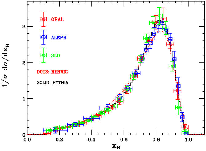
Figure 9.36: $B$-hadron spectrum measured by ALEPH, OPAL and SLD experiments, along with the HERWIG and PYTHIA predictions, after fitting the hadronization parameters to the data.

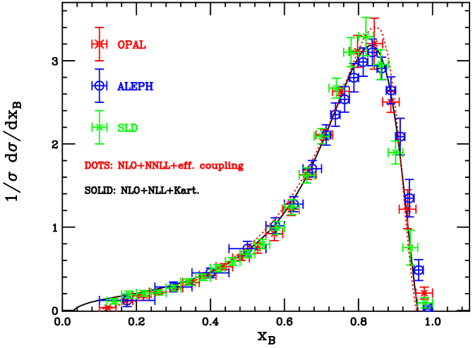
Figure 9.37: As in Fig. 9.36, but comparing the data with the NLO/NLL calculation using the Kartvelishvili hadronization model and the NLO/NNLL computation with the effective strong coupling constant.

We note in Fig. 9.36 that PYTHIA, after the tuning, gives a good description of the experimental spectra, while HERWIG’s distribution is broader, below the data around the peak and above them at small $x_{B}$. From Fig. 9.37, we learn that the NLO/NLL calculation using the Kartvelishvili model reproduces the data quite well, but it becomes negative at large $x_{B}$. The plot relying on the effective-coupling model lies above the data around the peak and approaches zero more rapidly at large $x_{B}$. In any case, even this result is acceptable, considering that, when modelling power corrections by means of the effective coupling constant, we are not tuning any free parameter to the data.

Using the fits to LEP and SLD data, we can predict the $B$-hadron spectrum in other processes, such as top-quark decay ($t\to bW$) and the decay of the Standard Model Higgs boson $H\to b\bar{b}$. In Figs. 9.38 and 9.39 we show the predictions yielded by HERWIG, PYTHIA and the resummed calculation based on the perturbative fragmentation approach for $B$-hadron production in top ($t\to bW$) and Higgs ($H\to b\bar{b}$) decays. We parametrize cluster, string and Kartvelishvili models using the best fits to LEP and SLD data. As for the resummation, we use the NLO/NLL calculations in Refs. [23, 24] for top decay and in Ref. [25] for $H\to b\bar{b}$ processes. In our plots we have set the top and Higgs masses to the values $m_{t}=175$ GeV and $m_{H}=120$ GeV. The results in Figs. 9.38 and 9.39 exhibit similar features to the comparison presented in Figs. 9.36 and 9.37: PYTHIA and the NLO/NLL calculation using the Kartvelishvili model are in good agreement, while the spectra yielded by HERWIG show some discrepancy, as they are broader than the other two predictions and lie below them at small $x_{B}$ and above at large $x_{B}$.

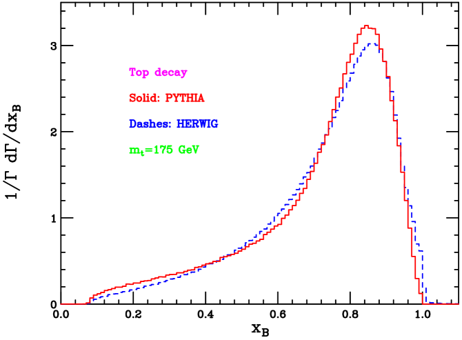
Figure 9.38: $B$-hadron spectrum in top quark decay according to HERWIG, PYTHIA and the NLO/NLL calculation which includes non-perturbative corrections via the Kartvelishvili hadronization model.

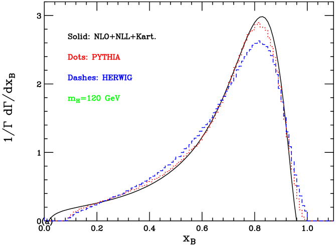
Figure 9.39: As in Fig. 9.38, but for $b$-flavoured hadron production in the decay of the Standard Model Higgs $H\to b\bar{b}$.

Finally, we present the same comparison in moment space, where the moments of the differential cross section are defined as follows:

$$\sigma_{N}=\int_{0}^{1}{dz\ z^{N-1}{1\over{\sigma}}{{d\sigma}\over{dz}}(z)}.$$ (9.37)

In Ref. [4], the DELPHI collaboration presented the first five moments for $B$ production in $e^{+}e^{-}$ annihilation. From the point of view of resummed calculations, working in moment space [26] presents several advantages. In $N$-space, convolutions become ordinary products, and the relation between parton- and hadron-level cross sections becomes: $\sigma_{N}^{B}=\sigma_{N}^{b}D_{N}^{\mathrm{np}}$, where $\sigma_{N}^{b}$ and $\sigma_{N}^{B}$ are the moments of the $b$ and $B$ cross sections, and $D_{N}^{\mathrm{np}}$ is the $N$-space counterpart of the non-perturbative fragmentation function. Therefore, there is no need to assume any functional form for the non-perturbative fragmentation function in $x_{B}$-space.

Table 9.11: Moments $\sigma^{B}_{N}$ from DELPHI [4], and $N$-space results in $e^{+}e^{-}$ annihilation, Higgs ($H$) and top ($t$) decay, according to NLO/NLL calculations, HERWIG (HW) and PYTHIA (PY). Also presented are the $N$-space $e^{+}e^{-}$ results obtained using the effective coupling constant $\tilde{\alpha}_{S}$ along with the theoretical errors [6].

	$\langle x\rangle$	$\langle x^{2}\rangle$	$\langle x^{3}\rangle$	$\langle x^{4}\rangle$
$e^{+}e^{-}$ data $\sigma_{N}^{B}$	0.715$\pm$0.005	0.540$\pm$0.006	0.424$\pm$0.007	0.341$\pm$0.006
$e^{+}e^{-}$ NLL $\sigma_{N}^{b}$	0.780	0.644	0.548	0.476
$D^{\mathrm{np}}_{N}$	0.917	0.839	0.773	0.716
$e^{+}e^{-}$ HW	0.711	0.535	0.418	0.335
$e^{+}e^{-}$ PY	0.716	0.541	0.424	0.340
$e^{+}e^{-}$ NNLL+$\tilde{\alpha}_{S}$	$0.687\pm 0.040$	$0.5019\pm 0.047$	$0.381\pm 0.046$	$0.298\pm 0.046$
$t$-dec. NLL	0.723	0.556	0.443	0.363
$t$-dec. HW	0.733	0.570	0.461	0.381
$t$-dec. PY	0.722	0.559	0.449	0.369
$H$-dec. NLL	0.695	0.517	0.402	0.321
$H$-dec. HW	0.684	0.504	0.388	0.308
$H$-dec. PY	0.688	0.508	0.391	0.310

The results of our $N$-space analysis are summarized in Table 9.11. We note that, after the fits to LEP and SLD data, HERWIG and PYTHIA agree with the DELPHI moments, within the experimental uncertainties. As for the calculation based on the effective coupling constant, it is able to reproduce the experimental moments within the theoretical errors which were calculated in [6] and quoted in Table 9.11. As done for the $x_{B}$-space analysis, we also present in Table 9.11 the moments of the differential width for the production of $B$ hadron in top or Higgs decays, using the moments $D_{N}^{\mathrm{np}}$ taken from the fits to the DELPHI data.

In summary, we studied bottom-quark fragmentation in $e^{+}e^{-}$ annihilation, top and Higgs decays using resummed calculations and the HERWIG and PYTHIA parton shower models. We fitted the Kartvelishvili, cluster and string models to $B$-hadron spectra measured at LEP and SLD, and then predicted the $B$-energy distribution in other processes. We also presented the results yielded by a model which incorporates non-perturbative power corrections via an effective strong coupling constant. The analysis was finally extended to Mellin moment space. We believe that the study here presented can be a useful starting point to address $b$-quark fragmentation at present and future colliders, as it sets some benchmarks for the hadronization models which are typically used along with Monte Carlo generators and resummed computations.

Monte Carlo simulations of top-quark pair production in hadronic collisions

M.Treccani

10.40 Introduction

In view of the starting of the LHC and the accumulated statistics at Tevatron, there appears the need for further improvement in the accuracy of theoretical predictions. One of the most interesting fields refer to the class of events with multiple final states, giving rise to multiple jets with complicated topologies. There exists different strategies to tackle this problem, with distinct features and points of strength. The main problem is how to consistently compose the contributions due to Matrix Element (ME) calculations with the contributions of the Monte Carlo showering codes (MC), in order to exploit their complementariety and avoid at the same time the so-called double counting phenomenon [1].
One of these strategies, known as MC@NLO, put the emphasis on achieving the next-to-leading-order (NLO) accuracy in the description of the inclusive rates for a given final state $F$, accompanied by the exact leading-order (LO) description of the emission of one extra jet ($F+$jet). For a detailed explanation of this approach and its implementation in several cases, see [2, 3, 4].
One alternative approach relies on a consistent leading-logarithmic (LL) accuracy in the prediction of a final state $F$ accompanied by a varying number of extra jets. The removal of double counting of jet is achieved by the so-called matching algorithm for matrix elements and parton shower. It is understood that the matching algorithm approach cannot improve the intrinsic LL accuracy of the predictions; however it will give a better accuracy in the prediction of the observables more sensible to the production of two or more jets in addition to $F$.
In this note, we study in detail the so-called MLM matching [5, 6] embedded in the the ME generator ALPGEN [7] in the $t\bar{t}$ pair production at hadron colliders. First we will address its stability w.r.t its internal parameters, and after we will perform detailed numerical comparison between MLM matching and the MC@NLO code.
In particular, in Section 2 we will perform some robusteness test on the ALPGEN calculations, comparing predictions obtained with different parameters and discussing the related uncertainties. Section 3 covers the detailed comparison between ALPGEN and MC@NLOpredictions, and in Section 4 we will present our conclusions.

10.41 Consistency studies of the matching algorithm

In this section we study the overall consistency of the matching algorithm applied to the case of $t\bar{t}$ final states. We shall consider $t\bar{t}$ production at the Tevatron ($p\bar{p}$ collisions at $\sqrt{S}=1.96$ TeV) and at the LHC ($pp$ collisions at $\sqrt{S}=14$ TeV).
The generation parameters for the light partons are defined by the following kinematical cuts: the default values for the event samples at the Tevatron (LHC) are given by:  $p_{\scriptscriptstyle T}^{\scriptscriptstyle{min}}$=20 (30) $\mathrm{GeV}$and $R_{\scriptscriptstyle{min}}$=0.7 (0.7), while they are considered only in the geometrical region defined by $\eta\leq 4(5)$.
The top particle is assumed to be stable, and therefore all jets coming from the decay of top quarks are neglected. For the shower evolution we use HERWIG, version 6.510 [8]. We stopped the evolution after the perturbative phase, in order to drop down all the common systematics that could smooth out any possible discrepancy between the various simulations. For all generations we chose the parton distribution function set MRST2001J[9], with renormalization and factorization scales squared set equal to: $\mbox{$\mu^{2}_{\rm R}$}=\mbox{$\mu^{2}_{\rm F}$}=\sum_{i=t,\bar{t},\mathrm{jets}}\;[m_{i}^{2}+(p_{\scriptscriptstyle T}^{i})^{2}]$. Jet observables are built out of the partons emerging form the shower in the rapidity range $|\eta|\leq 6$ and adopting the cone algorithm GETJET[10]. The jet cone size is set to $\mbox{$R_{\scriptscriptstyle{cone}}$}=0.7$ and the minimum transverse momentum to define a jet at the Tevatron(LHC) is 15(20) $\mathrm{GeV}$ .
Having defined the environmental parameters of these studies, we then explore the systematic uncertainties due to the variation of the internal parameters. These uncertainties reflect the underlying fact that this approach relies on the LO evaluation of the hard ME and on the LL accuracy in the removal of double counting and in the description of the shower evolution. In this section we shall show that the size of the resulting uncertainties is consistent with what can be expected in such a LL approach in the case of $t\bar{t}$ production.

To our analysis, the important feature of the whole procedure is the presence of two set of parameters: the generation cuts and the matching cuts (see [5, 6]). The first set is necessary to avoid the Infra-Red (IR) and collinear singularities:$p_{\scriptscriptstyle T}^{\scriptscriptstyle{min}}$ , the minimum transverse momentum of the extra-parton(s) to be generated, and $R_{\scriptscriptstyle{min}}$, the minimum separation between extra-partons in the $(\eta,\phi)$ plane. Along with these parameters, there exist an analogous set, but with slightly different meaninings : the matching cuts $E^{\scriptscriptstyle{clus}}_{\scriptscriptstyle T}$ and $R_{\scriptscriptstyle{match}}$. It’s worth to stress that the latter parameters are necessary to effectively separate the phase space, but the prediction should be stable against (slight) modifications of them, together with the choice of the particular cone jet algorithm adopted in the matching procedure.

In our examples here we consider two independent variations of the generation and of two of the matching cuts, as in table 10.12, keeping fixed our definition of the physical objects (the jets) and of the observables.

Then we proceed to study some distributions for the Tevatron, showing the observables dominated by contributions with up to 1 hard parton in fig. 10.40, and those relative to multijet final states in fig. 10.41. We find that these distribution are stable against reasonable variations of the internal parameters, with relative differencies confined well below few percents, both in matching and generation parameter variations. Angular observables, such as $\Delta R$, are more sensible, since they are directly related to the matching variables, and their agreement is within 10%.

	Generation parameters		Matching parameters
Param set	$p_{\scriptscriptstyle T}^{\scriptscriptstyle{min}}$	$R_{\scriptscriptstyle{min}}$	min $E^{\scriptscriptstyle{clus}}_{\scriptscriptstyle T}$	$R_{\scriptscriptstyle{match}}$
Tevatron, default	20	0.7	25	1.5 $\times$ 0.7
Tevatron, Set G1	15	0.7	20	1.5 $\times$ 0.7
Tevatron, Set G2	30	0.7	36	1.5 $\times$ 0.7
Tevatron, Set M1	20	0.7	20	1.5 $\times$ 0.7
Tevatron, Set M2	20	0.7	25	1.5 $\times$ 1.0
LHC, default	30	0.7	36	1.5 $\times$ 0.7
LHC, Set G1	25	0.7	30	1.5 $\times$ 0.7
LHC, Set G2	40	0.7	48	1.5 $\times$ 0.7
LHC, Set M1	30	0.7	30	1.5 $\times$ 0.7
LHC, Set M2	30	0.7	36	1.5 $\times$ 1.0

Table 10.12: Variations of the generation and matching parameters used for the study of the systematics.

Figure 10.40: Comparison between the three alternative sets of generation (left) and matching (right) parameters given in table 10.12, at the Tevatron.

Figure 10.41: Comparison between the three alternative sets of generation and matching parameters given in table 10.12, for multijet distributions at the Tevatron.

The analysis at the LHC, which will not be shown here, leads to qualitatively and quantitatively similar results.

10.42 Comparisons with MC@NLO

We shall now compare in detail the description of $t\bar{t}$ events as provided by ALPGEN  and MC@NLO. For consistency with the MC@NLO approach, where only the ${\cal O}(\alpha_{s}^{3})$ ME effects are included, we use ALPGEN  samples obtained by stopping the ME contributions only to 1 extra-parton besides the $t\bar{t}$ pair. This strategy allow to highlight the different features of the two alternative approaches applied to same set of contributions. It is understood that a homogeneous comparison can only be done through the introduction of a proper K factor, determined by the ratio of the total rates of the two predictions. We adopt the same simulation setup, modifying only the same factorization and renormalization scale in order to match MC@NLO’s default:
$\mbox{$\mu^{2}_{\rm R}$}=\mbox{$\mu^{2}_{\rm F}$}=\sum_{i=t,\bar{t}}\;{1\over 2}[m_{i}^{2}+(p_{\scriptscriptstyle T}^{i})^{2}].$

Figure 10.42: Comparison of ALPGEN (histogram) and MC@NLO (plot) distributions, at the Tevatron. The ALPGEN results are rescaled to MC@NLO, using the K factor of 1.36. The relative difference (MC@NLO-ALPGEN)/ALPGEN) is shown at the bottom of each plot.

The upper two rows of plots in figs. 10.42 refer to inclusive properties of the $t\bar{t}$ system, namely the transverse momentum and rapidity of the top and anti-top quark, the transverse momentum of the $t\bar{t}$ pair, and the azimuthal angle $\Delta\phi^{\scriptscriptstyle t\overline{\scriptscriptstyle t}}$ between the top and anti-top quark. The overall agreement is good, once ALPGEN  is corrected with the proper K-factor (1.36 for the Tevatron, and 1.51 for the LHC), and no large discrepancy is seen between the two descriptions of the chosen distributions. The most significant differencies (10 to 20%) are seen in the $p^{\scriptscriptstyle{top}}_{\scriptscriptstyle T}$ distribution, ALPGEN’s one being slightly softer.

The study of jet quantities reveals instead one important difference: the rapidity of the leading jet, $y_{{\scriptscriptstyle 1}}$, is different in the two descriptions, where MC@NLO  exhibits a dip at $\mbox{$y_{{\scriptscriptstyle 1}}$}=0$. This difference is particularly marked at the Tevatron, but is very visible also at the LHC. This is shown in the right figure of the third row in fig. 10.42 Visible differences are also present in the distribution of the 1st and 2nd jet separation in $(\eta,\phi)$ space, $\Delta R_{1,2}$.

Figure 10.43: Contributions to the transverse momentum of the leading jet in MC@NLO. Tevatron (left) and LHC (right).

Figure 10.44: Rapidity of the leading jet $y_{{\scriptscriptstyle 1}}$ at Tevatron for for various jet $p_{\scriptscriptstyle T}$ thresholds. Upper set: MC@NLO, with partial contributions. Central set: HERWIG. Lower set: comparison between ALPGEN, MC@NLO, and the parton level predictions

To understand the difference in the rapidity distribution, we look in more detail in fig. 10.43 at some features in the MC@NLO description of the leading jet. For the $p_{\scriptscriptstyle T}$ of the leading jet, $p_{\scriptscriptstyle T,1}$, we plot separately the contribution from the various components of the MC@NLO generation: events in which the shower is initiated by the LO $t\bar{t}$ hard process, and events in which the shower is initiated by a $t\bar{t}+q(g)$ hard process. In this last case, we separate the contribution of positive- and negative-weight events, where the distribution of negative events is shown in absolute value. The plots show that for MC@NLO  the contribution of the $t\bar{t}+q(g)$ hard process is almost negligible over most of the relevant range and becomes appreciable only for very large values of $p_{\scriptscriptstyle T,1}$. This hierarchy is stronger at the LHC than at the Tevatron.

Upper set of fig. 10.44 shows the various contributions to the rapidity distribution $y_{{\scriptscriptstyle 1}}$ for different jet $p_{\scriptscriptstyle T}$ thresholds. It appears that the $y_{{\scriptscriptstyle 1}}$ distribution resulting from the shower evolution of the $t\bar{t}$ events in MC@NLO has a strong dip at $y_{{\scriptscriptstyle 1}}$=0, a dip that cannot be compensated by the more central distributions of the jet from the $t\bar{t}+q(g)$ hard process, given its marginal role in the overall jet rate.

That the dip at $y_{{\scriptscriptstyle 1}}$=0 is a feature typical of jet emission from the $t\bar{t}$ state in HERWIG is shown in central set of fig. 10.44, obtained from the standard HERWIG code rather than from MC@NLO. We speculate that this feature is a consequence of the dead-cone description of hard emission from heavy quarks implemented in the HERWIG shower algorithm. To complete our analysis, we show in lower set of fig. 10.44 the comparison between the ALPGEN, MC@NLO and the parton-level $y_{{\scriptscriptstyle 1}}$ spectra, for different jet $p_{\scriptscriptstyle T}$ thresholds. We notice that at large $p_{\scriptscriptstyle T}$, where the Sudakov effects that induce potential differences between the shower and the PL results have vanished, the ALPGEN result reproduces well the PL result, while still differing significantly from the MC@NLO distributions.

10.43 Conclusions

The study presented in this paper examines the predictions of ALPGEN and its matching algorithm for the description of $t\bar{t}$+jets events. Several checks of the algorithm have shown its internal consistency, and indicate a rather mild dependence of the results on the parameters that define it. The consistency of the approach is confirmed by the comparison with MC@NLO. In particular, inclusive variables show excellent agreement, once the NLO/LO $K$ factor is included.
Instead we found a rather surprising difference between the predictions of two codes for the rapidity distribution of the leading jet accompanying the $t\bar{t}$ pair. In view of the relevance of this variable for the study at the LHC of new physics signals, it is important to further pursue the origin of this discrepancy, with independent calculations, and with a direct comparison with data. Preliminary results obtained with the new positive-weight NLO shower MC introduced in [11, 12] and presented in this Meeting [13], appear to support the distributions predicted by ALPGEN.

———————————————————————-

Phenomenology of the Standard Model Higgs boson at the LHC

G. Corcella and D. Rebuzzi

The Higgs boson plays a crucial role in the Standard Model (SM) of electroweak interactions, as it is responsible of the mechanism of mass generation. However, this particle has not yet been experimentally discovered. Searches for the Higgs boson will be one of the main goals of the Large Hadron Collider, which will be capable of exploring the Higgs mass spectrum from 100 GeV to about 1 TeV. In order to accurately perform such searches, the use of precise QCD calculations and reliable Monte Carlo event generators will be mandatory.

We study several observables related to the phenomenology of the SM Higgs boson and compare the predictions yielded by HERWIG [1] and PYTHIA [2], the two most popular event generators, as well as QCD computations resumming the large logarithms appearing in the Higgs transverse momentum spectrum [3]. In fact, some differences between HERWIG and PYTHIA are to be expected, since they implement parton showers [4, 5], matrix-element matching [6, 7] and hadronization [8, 9] in a different fashion (see [10] for some discussions and comparison between the two Monte Carlo codes). Hereafter we shall use the HERWIG 6.510 and PYTHIA 6.403 versions. As parton distribution functions (PDFs), the leading-order (LO) CTEQ6L1 set [11] will be employed.

We shall consider Higgs production via gluon-gluon fusion (GGF), which is the dominant channel at the LHC, and through vector-boson fusion (VBF). In HERWIG, the same user-defined process simulates both $gg\to H$ and $q\bar{q}\to H$, while in PYTHIA the two subprocesses can be run separately. In the following, for the sake of comparison, we shall use a modified version of HERWIG, with the $q\bar{q}\to H$ subprocess turned off. We checked that, with the PDF set [11], HERWIG simulates about 6–7% of events according to $q\bar{q}\to H$.

Indeed, if we compare the HERWIG and PYTHIA total cross sections for $gg\to H$, using the default parametrizations, we find meaningful discrepancies, about 15–20% for a Higgs mass $110~{}\mathrm{GeV}<m_{H}<190~{}\mathrm{GeV}$. We investigated the possible causes determining such differences and understood that they are mostly due to the value of the strong coupling constant $\alpha_{S}(m_{H})$ implemented in the two programs. Both codes tuned the QCD parameter $\Lambda$ to LEP data, along with other quantities, such as the shower cutoff, quark and gluon effective masses and the hadronization non-perturbative parameters. However, such fits led to pretty different results for the strong coupling constant at the $Z$ mass: $\alpha_{S}(m_{Z})\simeq 0.116$ in HERWIG and $\alpha_{S}(m_{Z})\simeq 0.127$ in PYTHIA. While the value of HERWIG is consistent with the world average, i.e. $\alpha_{S}(m_{Z})=0.118\pm 0.002$ [12], PYTHIA uses a somewhat higher value. Different values of $\alpha_{S}(m_{Z})$ clearly do not affect the total LO $e^{+}e^{-}\to q\bar{q}$ cross section, but do have an impact on the LO $gg\to H$ one, which is ${\cal O}(\alpha_{S}^{2}(m_{H}))$. Another difference between the two codes is the implementation of the QCD beta function, which is at two loops in HERWIG and at one loop in PYTHIA. At hadron colliders, while HERWIG still uses its own value of $\alpha_{S}(m_{Z})$, PYTHIA employs, for the hard process and the initial-state parton cascade, the same value of $\alpha_{S}(m_{Z})$ as the one in the chosen PDF. The LO CTEQ6L1 set uses $\alpha_{S}(m_{Z})=0.130$, even larger than the PYTHIA default, and much above the world average. In any case, we point out that, since HERWIG and PYTHIA yield only LO rates, they should not be used to calculate the Higgs production total cross section, which is currently available up to next-to-next-to-leading order (NNLO) [13]. Parton showers predict instead more reliably differential distributions, which exhibit milder dependence on $\alpha_{S}(m_{Z})$, since they are equivalent to resummations (see [14] for some comparison between Monte Carlo algorithms and resummed computations). Throughout our analysis we shall nonetheless use the same value of $\alpha_{S}(m_{H})$ in both HERWIG and PYTHIA. For example, we can employ, as a reference point, the value $\alpha_{S}(m_{Z})=0.130$, as in the parton density [11], leading to $\alpha_{S}(m_{H})\simeq 0.123$ using one-loop evolution from $m_{Z}$ to $m_{H}$. In HERWIG, in order to increase $\alpha_{S}(m_{Z})$, we shall have to increase the parameter QCDLAM (default value 0.18 GeV), which roughly corresponds to QCD quantity $\Lambda$ in the $\overline{\mathrm{MS}}$ renormalization scheme at high momentum fractions [14]. However, QCDLAM cannot be made arbitrarily large without modifying other HERWIG non-perturbative parameters, such as the shower cutoffs for gluons and quarks, namely VGCUT (default 0.10 GeV) and VQCUT (default 0.48 GeV). We found that a possible combination yielding $\alpha_{S}(m_{H})=0.123$ in HERWIG is the following:

$$\rm{QCDLAM}=0.378\ \rm{GeV}\ ;\ VGCUT=1.00\ \rm{GeV}\ ;\ VGCUT=1.50\ \rm{GeV}.$$ (11.38)

It can be seen that using the parametrization (11.38) in HERWIG the two programs give approximately the same rates, as shown in Table 11.13, where we quote the total cross section given by default PYTHIA (PY) and HERWIG (HW), and by HERWIG tuned according to Eq. (11.38) (HW^∗). Of course, one can also modify the PYTHIA parameters in order to have the same $\alpha_{S}(m_{H})$ as in HERWIG. Before moving on, we point out that we are aware that changing the default parameters of a Monte Carlo program can be dangerous, as this may likely spoil the agreement with the data taken into account in the fits. In fact, we are not recommending that one should use a different parametrization, such as Eq. (11.38), but just trying to understand the reason of the discrepancy and whether it is possible to improve the agreement between HERWIG and PYTHIA.

Table 11.13: Cross sections for Higgs production in the gluon-fusion channel, according to PYTHIA (PY) and HERWIG (HW), using their default parametrization, and according to HERWIG, tuned as in Eq. (11.38) (HW^∗).

$m_{H}$	$\sigma$ (PY)	$\sigma$ (HW)	$\sigma$ (HW∗)
110 GeV	20.7 pb	16.6 pb	20.2 pb
130 GeV	15.5 pb	13.2 pb	15.5 pb
150 GeV	12.2 pb	10.2 pb	12.2 pb
170 GeV	10.3 pb	7.9 pb	10.7 pb
190 GeV	7.9 pb	6.6 pb	8.1 pb

Table 11.14: Total Higgs decay width according to PYTHIA and HERWIG, using its default parameters and the tuning (11.38).

$m_{H}$	$\Gamma$ (PY)	$\Gamma$ (HW)	$\Gamma$ (HW∗)
110 GeV	2.5 MeV	3.5 MeV	3.0 MeV
130 GeV	4.4 MeV	5.4 MeV	4.8 MeV
150 GeV	15.8 MeV	16.4 GeV	15.6 GeV
170 GeV	355.2 MeV	328.6 MeV	337.3 MeV
190 GeV	981.6 MeV	919.3 MeV	919.6 MeV

As far as the decays of the Higgs boson are concerned, we investigated both the total width as well as the partial rates into a few given channels.. The total rates yielded by HERWIG and PYTHIA, even after tuning HERWIG as in Eq. (11.38), are a bit different, as quoted in Table 11.14. Several issues contribute to the discrepancy exhibited by Table 11.14. For example, the treatment of the decay $H\to ZZ$, on which our study will be later on mostly concentrated, is quite different in the two codes. While PYTHIA implements the general case, where both $Z$ bosons are allowed to be off-shell, in HERWIG at least one $Z$ is forced to be on-shell. We checked that if we selected events where both $Z$’s are on the mass shell, e.g. within five widths, HERWIG and PYTHIA rates would agree up to a good accuracy level.

We present in Table 11.15 the $H\to ZZ$ rates according to PYTHIA, HERWIG and HDECAY, a code, based on Ref. [15], computing the total and partial Higgs decay rates, possibly including higher-order radiative corrections. We note reasonable agreement between PYTHIA and HDECAY, which also permits that both $Z$’s are off-shell, while HERWIG yields slightly lower widths.

Among the other Higgs decay modes, major differences between HERWIG and PYTHIA are present especially in the channels into heavy quarks, such as $H\to c\bar{c}$ or $H\to b\bar{b}$, where the discrepancies between the two default codes can be up to $\sim 50\%$. Considering, e.g., the decay $H\to b\bar{b}$, both HERWIG and PYTHIA implement the $b$-quark $\overline{\mathrm{MS}}$ mass $\bar{m}_{b}(m_{H})$, which is an appropriate mass definition for $b\bar{b}$ production at the Higgs mass scale. However HERWIG, unlike PYTHIA, also includes the leading-logarithmic (LL) resummation of the large contributions $\sim\alpha_{S}^{n}(m_{H})\ln^{n}(m_{H}/m_{b})$ and NLO corrections to $\bar{m}_{b}(m_{H})$. Removing such higher-order corrections, and still using the tuning (11.38), we expect that HERWIG and PYTHIA should agree. The partial rates of the two Monte Carlo generators can again be compared with the results of the HDECAY code. In the $H\to b\bar{b}$ mode, HDECAY includes the NNLO corrections to the $\overline{\mathrm{MS}}$ $b$-quark mass, the NLO ones to the massive rate $\Gamma(H\to b\bar{b})$ near threshold, and even the NNNLO ones, in the massless approximation $m_{b}\ll m_{H}$, far above threshold. We present in Table 11.16 the widths for $H\to b\bar{b}$ according to HERWIG, PYTHIA and HDECAY for few values of $m_{H}$ and using $\alpha_{S}(m_{H})=0.123$ everywhere. HERWIG yields the largest rate, even above the HDECAY result; hence, we may conclude that some of the higher-order corrections that HDECAY implements, whereas HERWIG does not, have negative sign. We finally remark that, unlike HERWIG, PYTHIA includes the modes $H\to gg$ and $H\to\gamma Z^{*}$.

Table 11.15: Width $\Gamma(H\to Z^{(*)}Z^{(*)})$ for different values of $m_{H}$ according to PYTHIA, HERWIG with the parametrization (11.38) and HDECAY, for several values of the Higgs boson mass

$m_{H}$	$\Gamma$ (PY)	$\Gamma$ (HW∗)	$\Gamma$ (HDECAY)
110 GeV	0.012 MeV	0.011 MeV	0.012 MeV
120 GeV	0.053 MeV	0.051 MeV	0.054 MeV
130 GeV	0.186 MeV	0.173 MeV	0.189 MeV
140 GeV	0.530 MeV	0.503 MeV	0.541 MeV
150 GeV	1.357 MeV	1.311 MeV	1.374 MeV

Table 11.16: As in Table 11.15, but for the decay $H\to b\bar{b}$.

$m_{H}$	$\Gamma$ (PY)	$\Gamma$ (HW∗)	$\Gamma$ (HDECAY)
110 GeV	1.88 MeV	2.46 MeV	2.23 MeV
130 GeV	2.17 MeV	2.82 MeV	2.55 MeV
150 GeV	2.46 MeV	3.18 MeV	2.85 MeV
170 GeV	2.74 MeV	3.51 MeV	3.15 MeV
190 GeV	3.02 MeV	3.84 MeV	3.44 MeV

As anticipated, in our phenomenological analysis we shall consider SM Higgs production in GGF and VBF and concentrate ourselves mostly on the decay channel $H\to ZZ\to 4\ell$. We shall study the following distributions: the $Z$- and $H$-boson mass spectrum, the Higgs and $Z$ transverse momentum ($q_{T,H}$ and $q_{T,Z}$) and pseudorapidity ($\eta_{H}$ and $\eta_{Z}$). Such spectra are presented in Figs. 11.45–11.49, for a Higgs mass $m_{H}=130$ GeV.

The $m_{H}$ distributions of HERWIG and PYTHIA (Fig. 11.45) look compatible. On the contrary, the fact that PYTHIA allows both $Z$’s to be off-shell has an evident impact on Fig. 11.46: in the intermediate $Z$-mass range, say 40–80 GeV, where both $Z$’s are off-shell, and PYTHIA yields more events. Once again, if we set a filter allowing only $Z$’s near the mass shell, the discrepancies in the intermediate $m_{Z}$ range will disappear. In Fig. 11.47 we instead compare the $Z$ transverse momentum distributions: in GGF PYTHIA predicts more events than HERWIG at large $q_{T}$, while in VBF the two codes roughly agree. As we shall discuss later in more detail, for the time being, the default version of PYTHIA includes matrix-element corrections to Higgs production in GGF, while HERWIG does not. Such corrections are responsible of the simulation of a few events with a Higgs of large transverse momentum, whose decays still yield $Z$’s at large $q_{T}$. In Fig. 11.48 we instead present the Higgs pseudorapidity distributions: we clearly note an asymmetry, about 5%, for VBF in HERWIG, with more events simulated at positive rather than negative $\eta_{H}$. PYTHIA yields instead a symmetric spectrum. This asymmetry exhibited by HERWIG is currently under investigation [16] and should be clarified in a forthcoming publication [17]. As for the $\eta_{H}$ distribution in GGF, both HERWIG and PYTHIA spectra are symmetric, although some discrepancy is still present, with PYTHIA leading to more events around $\eta_{H}=0$. The HERWIG and PYTHIA $Z$-pseudorapidity spectra, presented in Fig. 11.49, are instead rather similar.

Figure 11.45: Higgs invariant-mass distribution for $H\to ZZ$ decays and Higgs production in gluon-gluon (left) and vector-boson (right) fusion, according to HERWIG (solid line) and PYTHIA (dashes).

Figure 11.46: As in Fig. 11.45, but showing the $Z$-mass distribution.

Figure 11.47: $Z$ transverse momentum spectrum in GGF (left) and VBF (right).

Figure 11.48: Higgs pseudorapidity distribution in GGF (left) and VBF (right).

Figure 11.49: As in Fig. 11.48, but presenting the $Z$ pseudorapidity.

We finally wish to present results on the Higgs transverse momentum distribution, which has been thoroughly investigated using Monte Carlo generators as well as resummed calculations. In fact, the NLO Higgs $q_{T}$ spectrum exhibits contributions, $\sim\alpha_{S}^{n}\ln^{k}(m_{H}^{2}/q_{T}^{2})$, with $k\leq n+1$, which are large for small values of the Higgs transverse momentum. Small values of $q_{T}$ correspond to initial-state soft or collinear parton radiation. Such logarithms have been resummed in [3] up to next-to-next-to-next-to-leading logarithmic accuracy (NNLL) in a Sudakov-like exponential factor. The authors of Ref. [3] also released a computing code, named HqT, implementing numerically their resummation.

In detail, the LLs are $\sim\alpha_{S}^{n}\ln^{n+1}(m_{H}^{2}/q_{T}^{2})$, the NLLs $\sim\alpha_{S}^{n}\ln^{n}(m_{H}^{2}/q_{T}^{2})$, the NNLLs $\sim\alpha_{S}^{n}\ln^{n-1}(m_{H}^{2}/q_{T}^{2})$ and so forth. While at small $q_{T}$ the resummation works fine, at large $q_{T}$ one should rely on fixed-order calculations. The HqT code allows one to match the resummation with the fixed-order spectrum up to NNLO accuracy . As for HERWIG and PYTHIA, their standard algorithms [4, 5] are reliable for soft or collinear parton radiation, i.e. for Higgs production at small $q_{T}$. In fact, it can be shown [14] that parton showers include all soft/collinear leading logarithms, plus some NLLs as well. Higgs production at large $q_{T}$ corresponds instead to hard or large-angle initial-state radiation: therefore, it cannot be simulated by standard parton shower algorithms, but must be described by the use of the exact tree-level NLO matrix-element [18, 19].

In order to allow hard and large-angle radiation, HERWIG and PYTHIA have been provided with matrix-element corrections [6, 7], although their actual implementation is indeed somewhat different. HERWIG splits the phase space into two regions: a region corresponding to soft/collinear emission, where one uses the parton shower approximation, and a region associated with hard or wide-angle radiation, the so-called ‘dead zone’ of the standard algorithm, where the exact tree-level amplitude is used. Moreover, the exact matrix element is also employed to correct the radiation in the HERWIG parton-shower region any time an emission is capable of being the hardest so far, i.e. it has the largest $q_{T}$ with respect to the radiating parton. Unlike HERWIG, PYTHIA uses instead the parton-shower approximation in all physical phase space and corrects with the exact amplitude only the first branching [7]. As discussed in [6], correcting only the first emission will however lead to an unphysical dependence of the hard-emission probability on the infrared cutoff, appearing in the Sudakov form factor.

The latest version of PYTHIA [2] does include matrix-element corrections to Higgs production in gluon-gluon fusion, though treating the top quark in the loop in the infinite-mass limit. The official version of HERWIG [1] does not include yet the corrections to Higgs production, although a preliminary code is available, based on the paper [20], which extends the earlier work for Drell–Yan processes [21]. With respect to PYTHIA, Ref. [20] fully includes top-quark mass effects and possibly corrects even to $q\bar{q}\to H$, whenever this subprocess is turned on. We also compare the Monte Carlo spectra with the HqT code, which we run in the NLL approximation, matched to the NLO total cross section in the point $q_{T}=m_{H}$. The results are presented in Fig 11.50, where we also show the result yielded by the HERWIG ‘Higgs+jet’ process, where the hard-scattering process is always generated according to one of the tree-level corrections to $gg\to H$, i.e. $gg\to Hg$, $qg\to Hq$, etc. We set in all codes $\alpha_{S}(m_{H})$ to the same value, however, at large $q_{T}$ still different scales $\mu$ for the strong coupling are used. In fact, by default, HERWIG uses the Higgs transverse mass $\mu=\sqrt{q_{T}^{2}+m_{H}^{2}}$, which is a reasonable scale since the dead zone corresponds to $q_{T}\geq m_{H}$; PYTHIA uses instead $\mu=q_{T}$; HqT sets $\mu=m_{H}$. For the sake of comparison, we set $\mu=q_{T}$ in all codes for $q_{T}\geq m_{H}$: this way, all spectra should roughly agree at large transverse momentum. From Fig. 11.50 we learn that the Higgs+jet spectrum roughly agrees with HqT at large $q_{T}$. The small discrepancy can be due to the fact that HqT also includes bottom quarks in the loop and to different choices of the PDF factorization scale, which is set to $\mu_{F}=m_{H}$ in HqT and $\mu_{F}=q_{T}$ in HERWIG and PYTHIA. The HERWIG and PYTHIA $q_{T}$ spectra, though in agreement with each other, are a bit below the other two curves, even though the same tree-level NLO matrix element has been used. Such a discrepancy obviously needs further investigation [17].

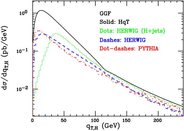
Figure 11.50: Transverse momentum distribution of the Higgs boson, produced in gluon fusion, according to HqT (solid line), HERWIG (dashed), PYTHIA (dot-dashed) and the HERWIG ‘Higgs+jet’ process (dotted).

In summary, we performed a study on SM Higgs boson production and decay at the LHC, mainly using PYTHIA and HERWIG, the two most popular Monte Carlo generators. We found several differences between the two codes: we understood the causes of most discrepancies, whereas a few are still under investigation. In a forthcoming work [17] we shall present an even more detailed analysis of Higgs boson phenomenology, where we shall also study the impact of the NLO corrections to Higgs production in GGF, implemented in the MC@NLO code [22].

MSSM Higgs Searches with CMS

G. Masetti

12.44 Introduction

According to the Minimal Supersymmetric Standard Model (MSSM), two isospin Higgs doublets have to be introduced. After electroweak symmetry breaking, five Higgs scalar mass eigenstates remain: one CP-odd neutral scalar boson A, two charged scalars $H^{\pm}$, and two CP-even neutral scalars h and H. At the tree level, the Higgs sector is completely defined by only two parameters: they are usually chosen as the ratio of the vacuum expectation values ($\tan\beta=v_{2}/v_{1}$) and the Higgs boson A mass ($M_{A}$). The tree level hierarchies ($M_{h}<M_{Z}$, $M_{A}<M_{H}$ and $M_{W}<M_{H}$) are modified by large radiative corrections: the leading one-loop correction is proportional to $m_{t}^{4}$ and the upper bound of $M_{h}$ is shifted to $M_{h}\leq 135~{}{\rm GeV/}c^{\rm 2}~{}$.

Varying $M_{A}$ in the range $91~{}{\rm GeV/}c^{\rm 2}~{}<M_{A}<1~{}{\rm TeV/}c^{\rm 2}~{}$ we can distinguish three different regimes:

• Decoupling regime. If $M_{A}\gg M^{max}_{h}$ then the Higgs bosons H, A and $H^{\pm}$ are very heavy and almost degenerate in mass, while h has a mass very close to $M^{max}_{h}$ and becomes SM-like. H and A, besides their masses, are degenerate also in width and cross section.

• Low $M_{A}$ regime. If $M_{A}<M^{max}_{h}$ the behavior of the two CP-even neutral Higgs bosons h and H is swapped with respect to the decoupling regime: h is almost degenerate in mass, width and cross section with A, and H is the SM-like Higgs, with a mass close to $M^{max}_{h}$.

• Intense coupling regime. This occurs for $M_{A}\sim M^{max}_{h}$ and high $\tan\beta$ [1, 2] and it leads to similar, but not degenerate, masses for the three neutral Higgs bosons. This property, in principle, allows to detect the three neutral Higgs separately.

Figure 12.51: Neutral MSSM Higgs production cross sections at the LHC.

The LEP experiments have excluded the Higgs masses $M_{A}<91.9~{}{\rm GeV/}c^{\rm 2}~{}$, $M_{h,H}<91~{}{\rm GeV/}c^{\rm 2}~{}$ [3] and $M_{H^{\pm}}<78.6~{}{\rm GeV/}c^{\rm 2}~{}$ [4].

In this report the discovery potential of the MSSM neutral Higgs boson with the CMS detector at LHC is presented. These analysis are also described in [5].

12.45 Neutral Higgs bosons searches

The production cross-section for the MSSM neutral Higgs bosons is strongly dependent on the value of the $\tan\beta$ parameter. All neutral MSSM Higgs production cross sections including NLO QCD corrections are shown in Fig.12.51.

12.45.1 Large $\tan\beta$

In the region with large $\tan\beta$ values ($>$ 15) the neutral Higgs bosons are mainly produced in association with b-quarks: $pp\rightarrow q\bar{q}/gg\rightarrow h/A/H+b\bar{b}$. The presence of a $b\bar{b}$ pair is important to suppress the very large background from Drell-Yan processes. The Higgs bosons mainly decay in a $b\bar{b}$ pair (90$\%$) and in a $\tau\bar{\tau}$ pair (10$\%$). In CMS six channels have been studied:

• $A/H\rightarrow\mu\mu$

• $A/H\rightarrow\tau\tau\rightarrow e+jet+X$

• $A/H\rightarrow\tau\tau\rightarrow\mu+jet+X$

• $A/H\rightarrow\tau\tau\rightarrow jet+jet+X$

• $A/H\rightarrow\tau\tau\rightarrow e+\mu+X$

• $A/H\rightarrow bb$

The muon final state, with respect to the other channels, has a much lower branching ratio ($\approx 3\times 10^{-4}$), but the event is very clean and Higgs masses and widths can be reconstructed precisely. Moreover it is possible to exploit the theoretical relation between the Higgs decay width and $\tan\beta$ ($\Gamma_{H}\propto\tan^{2}\beta$) to perform a direct measurement of this latter quantity.

The rejection strategy is mainly based on identification of isolated muons and on b-tagging. This latter selection is particular important: b jets from signal events are mainly produced in the forward region with lower $p_{T}$ with respect to the b jets coming from $t\bar{t}$ background. Figure 12.52 (left) shows the reconstructed dimuon invariant mass for signal and background.

The tau channels, on the other hands, have a better signal to background ratio and can reach larger discovery region in the plane ($M_{A},\tan\beta$), as can be seen in Fig. 12.54 (left). Fig. 12.52 (right) shows the reconstructed invariant mass for signal and background that can be obtained with the $A/H\rightarrow\tau\tau\rightarrow e+jet$ channel. Indeed, despite the escaping neutrino, the Higgs boson mass can be reconstructed also for these channels, exploiting the collinearity approximation: the neutrino is assumed to be emitted along the $\tau$ direction.

Finally, the bb channel must take into account the huge QCD background and, to perform a discovery, one needs to know in advance masses and widths of the Higgs bosons. Thus this channel can be considered mainly as a cross-check for the discovery.

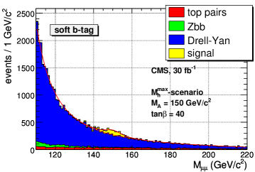
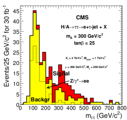
Figure 12.52: Reconstructed dimuon mass for the main background and for the signal sample with $M_{A}$ = 150$~{}{\rm GeV/}c^{\rm 2}~{}$ and $\tan\beta$ = 40 for the $A/H\rightarrow\mu\mu$ channel (left) and with $M_{A}$ = 300$~{}{\rm GeV/}c^{\rm 2}~{}$ and $\tan\beta$ = 25 for the $A/H\rightarrow\tau\tau\rightarrow e+jet$ channel (right).

12.45.2 Small $\tan\beta$

Concerning low $\tan\beta$ values, the dominant neutral MSSM Higgs production mechanism is the gluon fusion $gg\rightarrow h/A/H$, which can be mediated by top and botton loops (as in the SM case), but also by stop and sbottom (Fig.12.51).

In CMS two channels have been investigated:

• $A\rightarrow Zh\rightarrow\ell^{+}\ell^{-}b\bar{b}$

• $A/H\rightarrow\tilde{\chi}^{0}_{2}\tilde{\chi}^{0}_{2}\rightarrow 4\ell+E^{miss}_{T}$

The first channel provides an interesting way to detect A and h simultaneously. The cross section increases with decreasing of $\tan\beta$, while the mass range is $m_{Z}+m_{h}\leq m_{A}\leq 2m_{top}$. However results are strongly dependent on the MSSM parameters $\mu$ and $M_{2}$, because the Higgs boson decay $A\rightarrow\tilde{\chi}^{0}_{1}\tilde{\chi}^{0}_{1}$ may become dominant (the best results being obtained for large values of $\mu$ and $M_{2}$). Fig. 12.53 (left) shows the discovery region for this channel for 30 and 60$~{}\rm fb^{-1}~{}$ of integrated luminosity.

To increase the discovery region in the low and intermediate region of $\tan\beta$, the second channel has been studied which takes into account the decay modes of the neutral Higgs bosons to supersymmetric particles. The final state studied by this channel is particular clean (four leptons plus missing transverse energy). The analysis is performed in three benchmark points of the minimal Super Gravity constrained version of the MSSM (mSUGRA): these points are obtained varying the parameters $m_{0}$ and $m_{{1\over 2}}$ for $\tan\beta$ = 5, 10, $sign(\mu)$ = + and $A_{0}$ = 0. Fig.12.53(right) shows the discovery region in the ($m_{0},m_{{1\over 2}}$) plane, for an integrated luminosity of 30$~{}\rm fb^{-1}~{}$.

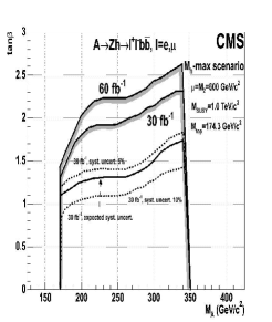
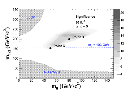
Figure 12.53: (left) The $5\sigma$ discovery region contours for 30 and 60 $~{}\rm fb^{-1}~{}$ integrated luminosity for the $A\rightarrow Zh$ channel. The effect of underestimation or overestimation of the background systematic uncertainty can be seen in the courve of 30 $~{}\rm fb^{-1}~{}$. (right)The $5\sigma$ discovery region contours for 30 $~{}\rm fb^{-1}~{}$ integrated luminosity for the $A/H\rightarrow\tilde{\chi}^{0}_{2}\tilde{\chi}^{0}_{2}$ channel.

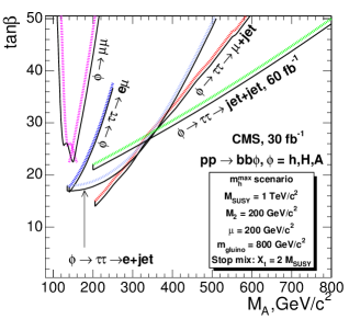
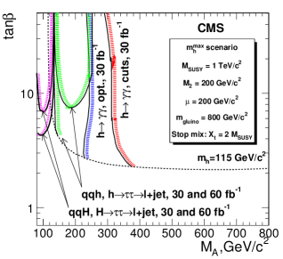
Figure 12.54: The 5$\sigma$ discovery regions for the neutral Higgs bosons $\phi$ ($\phi$=h, H, A) produced in the association with b quarks $\rm p\rm p\rightarrow\rm b\bar{\rm b}\phi$ with the $\phi\rightarrow\mu\mu$ and $\phi\rightarrow\tau\tau$ decay modes (left plot) and for the light, neutral Higgs boson h from the inclusive $\rm p\rm p\rightarrow\rm h$+X production with the $\rm h\rightarrow\gamma\gamma$ decay and for the light and heavy scalar Higgs bosons, h and H, produced in the vector boson fusion $\rm q\rm q\rightarrow\rm q\rm q\rm h(\rm H)$ with the $\rm h(\rm H)\rightarrow\tau\tau\rightarrow\ell$+jet decay (right plot). The $\rm m_{\rm h}^{\rm max}$ scenario is used.

Fig.12.54 summarize the $5\sigma$ discovery region that can be obtained with 30$~{}\rm fb^{-1}~{}$ of integrated luminosity.

12.46 Charged Higgs bosons searches

Three channels, depending on the final state and on the Higgs boson mass, have been investigated for charged Higgs bosons:

• $H^{\pm}\rightarrow\tau\nu_{\tau}$, with $M_{H}<M_{top}$

• $H^{\pm}\rightarrow\tau\nu_{\tau}$, with $M_{H}>M_{top}$

• $H^{\pm}\rightarrow tb$, with $M_{H}>M_{top}$

For Higgs boson masses below $M_{top}$, the main production mechanism is through top decay, $t\rightarrow H^{+}b$, and the branching ratio of the $\tau\nu$ channel is about 98% (Fig.12.55(left)). The study is performed considering the leptonic decay of the W: $t\bar{t}\rightarrow H^{\pm}W^{\mp}b\bar{b}\rightarrow\tau\nu_{\tau}\ell\nu_{\ell}b\bar{b}$, $\tau\rightarrow$ hadrons. The discovery region, as can be seen in figure 12.55(right), covers almost the entire allowed region in the ($M_{A},\tan\beta$) plane.

If $M_{H}>M_{top}$, the charged Higgs bosons are mainly produced in association with a top-bottom pair, $gg\rightarrow tbH^{\pm}$. The final state for this channel is very clean ($H^{\pm}\rightarrow\tau^{\pm}\nu$, $r\rightarrow hadrons+\nu$ and $W^{\mp}\rightarrow jj$) and, after the selection cuts, almost background free. The characteristics for this channel is the presence of large missing transverse energy and the $\tau$ helicity correlations favouring the $H^{\pm}\rightarrow\tau^{\pm}\nu$ decay over the $W^{\pm}\rightarrow\tau^{\pm}\nu$ decay. A large sector of the ($M_{A},\tan\beta$) plane can be covered (Fig.  12.55(right)).

Finally, for masses above $M_{top}+M_{bottom}$, the channel $H^{\pm}\rightarrow tb$ opens up. Two production mechanism are considered:

• $gb\rightarrow tH^{\pm}\rightarrow ttb\rightarrow W^{+}W^{-}bbb\rightarrow qq^{\prime}\mu\nu_{\mu}bbb$

• $gg\rightarrow tH^{\pm}b\rightarrow ttbb\rightarrow W^{+}W^{-}bbbb\rightarrow qq^{\prime}\mu\nu_{\mu}bbbb$

Unfortunately no sensitivity is obtained in the MSSM parameter space with this analysis, due to the large background and the resulting large effects of systematic uncertainties on its knowledge.

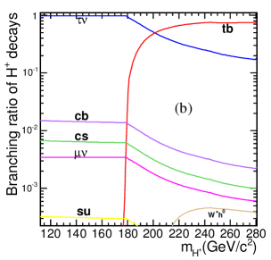
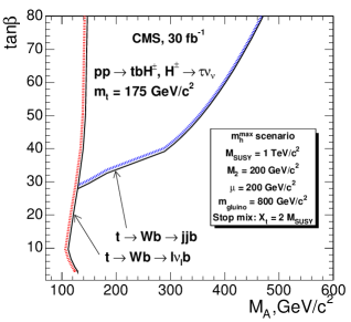
Figure 12.55: Branching ratios for charged Higgs boson decaying to different final states for $\tan\beta$ = 20 (left). The $5\sigma$-discovery regions for the charged Higgs boson with the $\tau\nu$ decay mode with 30$~{}\rm fb^{-1}~{}$ of integrated luminosity (right).

Fig.12.55(right) summarize the $5\sigma$ discovery region that can be obtained with 30$~{}\rm fb^{-1}~{}$ of integrated luminosity.

12.47 Conclusions

Many channels have been studied to estimate the discovery potential of MSSM Higgs bosons at CMS. A large area in the ($M_{A},\tan\beta$) plane will be explored: the most promising channels are $\phi\rightarrow\tau\tau$ ($\phi$ = h,A,H) and $H^{\pm}\rightarrow\tau\nu$.

Physics studies at the LHC with PHANTOM

G. Bevilacqua

13.48 Introduction

To shed light on the nature of Electroweak Symmetry Breaking (EWSB) is one among the main purposes of the LHC experiments. The Standard Model provides the most economical explanation in terms of the Higgs mechanism. The remarkable agreement between its predictions and precision electroweak data is consistent with a light Higgs boson with a mass lower than 200 GeV[1], while direct searches have established a lower bound of 114.4 GeV[2] at 95% CL.

The Higgs mechanism is essential to ensure the renormalizability of the Standard Model. Moreover, without a Higgs the theory is not self-consistent and violates perturbative unitarity at high energies, which implies that for several processes the amplitude grows indefinitely with energy. This unphysical behaviour is particularly manifest in the scattering of longitudinally polarized vector bosons, whose cross section goes over the unitarity limit at about one TeV. If the Higgs hypothesis is not realized, effects of new physics are expected to restore unitarity at this scale.

On the other side, if a massive Higgs boson exists, a resonance will be observed in the $VV$ invariant mass spectrum in correspondence of the Higgs mass. Vector Boson Fusion represents the second most important contribution to the cross section for Higgs production at LHC, moreover $H\rightarrow VV$ is the preferred decay channel above about 150 GeV. Final states in which the vector bosons decay into four leptons or two leptons plus two jets provide one of the cleanest signatures for Higgs detection.

It should be mentioned that even if a light Higgs will be discovered, the gauge boson scattering could nonetheless deviate from the Standard Model predictions in the high energy domain. Several models have been proposed, whereby the Higgs is a composite Goldstone boson associated to some new strong dynamics active at the TeV scale[3, 4]. The $VV$-scattering cross section is expected to be enhanced at high $M_{VV}$ as a consequence of the new strongly interacting sector.

In brief, Boson-Boson Scattering has a great potential for probing the mechanism of EWSB at LHC, independently of its particular realization. Unfortunately, no beam of on-shell bosons will be available. The only consistent way to extract some information from data is to rely upon a complete calculation of final states with six fermions.

A Monte Carlo event generator, PHANTOM[5], has been recently developed to provide a complete description at $\mathcal{O}(\alpha_{\scriptscriptstyle EM}^{6})+\mathcal{O}(\alpha_{\scriptscriptstyle EM}^{4}\alpha_{\scriptscriptstyle S}^{2})$ of all six-parton final states in the Standard Model, including for the first time all EW and mixed EW+QCD contributions at this perturbative order. Exact matrix elements at tree level are evaluated efficiently. A good coverage of phase space is achieved thanks to a new approach[6] which combines the best features of multichannel with the adaptivity of the VEGAS algorithm[7]. Apart from Boson-Boson Scattering and Higgs search, the program gives access to the full tree-level description of $t\bar{t}$ production which is important both in itself and as a background in connection with the previous topics.

In this note we present the first parton-level studies based on PHANTOM. The analysis is focused on Boson-Boson Scattering and Higgs search via Vector Boson Fusion in the semi-leptonic channels, that is final states characterized by four quarks and two charged leptons or one charged lepton plus one neutrino. A light Higgs scenario is compared with no-Higgs ($M_{H}\rightarrow\infty$) results, to be intended at this stage as a minimal benchmark in the search for new physics beyond the Standard Model.

13.49 Boson-Boson Scattering signature and its irreducible background

The problem of how to define a signal for Boson-Boson Scattering has been debated since a long time. Ideally, one should isolate the contribution of diagrams like the one depicted in Fig.13.56(a), in which the incoming partons emit two space-like vector bosons which scatter among themselves and finally decay into fermions. The resulting amplitude should then be deconvoluted from the PDF’s and finally projected to on-shell bosons. In practice, this procedure turns out to be problematic due to gauge invariance and cancellation effects. In fact the subset of boson-boson fusion diagrams is not separately gauge invariant and there are relevant negative interferences[8] with the rest of the diagrams, some of which are illustrated in Fig.13.56(b,c,d). Previous studies have evidentiated substantial differences among results based on this approximation and exact tree-level predictions on the $VV$ mass spectrum[9, 10], showing that a complete evaluation of all contributions at $\mathcal{O}(\alpha_{\scriptscriptstyle EM}^{6})$ is necessary.

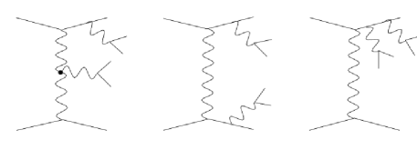
Figure 13.56: The Boson-Boson Scattering topology (a) and other typical contributions to the amplitude of a six-fermion final state (b,c,d).

In the two-step approach we follow, we first study the characteristics of Boson-Boson Scattering from a six-fermion point of view. As no contribution to $VV$ scattering can be found outside $\mathcal{O}(\alpha_{\scriptscriptstyle EM}^{6})$, it is convenient to start with a complete study of all processes at this perturbative order. In our intention, this represents a benchmark for physics analyses and does not claim to be fully realistic. With the help of appropriate selection cuts, we isolate a sample of events which best exemplifies the signature of the physical process under investigation. This means that candidates for top or three-boson production are subtracted to the advantage of events characterized by two tag jets widely separated in pseudorapidity and two couples of jets and leptons resonant at $W$ or $Z$ mass. Subsequently, further procedures are examined to enhance the contribution of longitudinally polarized vector bosons, which are most sensitive to effects of EWSB. The inclusion of the relevant QCD background represents the step forward which is essential to get meaningful results at parton level and completes our analysis.

Some examples of contributions to the QCD irreducible background are illustrated in Fig.13.57. Top production, either from single $t$ or $t\bar{t}$, is a huge source of background for this kind of studies. In particular $t\bar{t}$ is dominated by $\mathcal{O}(\alpha_{\scriptscriptstyle EM}^{4}\alpha_{\scriptscriptstyle S}^{2})$ contributions due to diagrams shown in Fig.13.57(a,b). $VV+2\,jets$ at $\mathcal{O}(\alpha_{\scriptscriptstyle EM}^{4}\alpha_{\scriptscriptstyle S}^{2})$ is another important background with a signature characterized by two outgoing vector bosons, quite similar to the scattering one and therefore particularly challenging to subract.

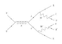
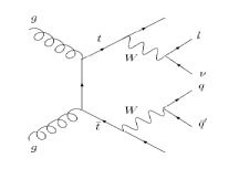
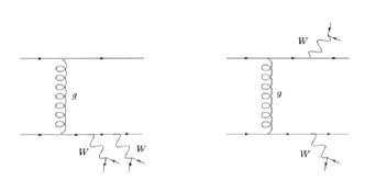
Figure 13.57: Examples of contributions to the QCD irreducible background: $t\bar{t}$ production (a,b) and $VV+2\,jets$ (c,d)

In the case of totally leptonic channels, i.e. final states with four leptons, $\mathcal{O}(\alpha_{\scriptscriptstyle EM}^{4}\alpha_{\scriptscriptstyle S}^{2})$ encompasses the full QCD background at tree level for six-fermion analyses. On the contrary, semileptonic channels get additional contributions from $\mathcal{O}(\alpha_{\scriptscriptstyle EM}^{2}\alpha_{\scriptscriptstyle S}^{4})$ diagrams which are responsible for the $V+4\,jets$ background. The latter must be included as well in a complete analysis and can be covered by other Monte Carlo event generators, such as AlpGen[11] or MadEvent[12]. It should be noticed nevertheless that these contributions have quite different kinematical features with respect to the scattering signature, therefore they are expected to be easily suppressed by means of appropriate selection cuts. Of course, the final word is left to the results of a complete study.

13.50 $\mathcal{O}(\alpha_{\scriptscriptstyle EM}^{6})$ results in the semileptonic $\mu^{+}\mu^{-}$ channel

This section is devoted to the analysis at $\mathcal{O}(\alpha_{\scriptscriptstyle EM}^{6})$ of all the processes of type $qq\rightarrow qqqq\mu^{+}\mu^{-}$. All our results have been obtained using the CTEQ5L[13] PDF set with scale

$$Q^{2}=M_{W}^{2}+{1\over 6}\,\sum_{i=1}^{6}p_{Ti}^{2},$$ (13.39)

where $p_{Ti}$ denotes the transverse momentum of the $i$-th final state particle.

As already mentioned, the choice to start from pure EW results is motivated by the fact that no QCD diagram contributes to the scattering topology. At this stage we are mainly concerned with isolating as much as possible the $VV$ scattering signature in the spirit of the discussion of the previous section. Following this approach, the selection procedure we adopt in this section makes use of flavour information and is not fully realistic. Results are found anyway to be not too sensitive to the details of the selection cuts, as shown in Fig.13.58. We compare different methods of reconstructing the $VZ$ invariant mass. Results based on flavour selection and predictions obtained using cuts on the invariant mass only are shown. The two distributions differ by about 20% at small invariant masses but agree quite nicely above 800 GeV, showing that results based on flavour information are not seriously degraded when selection procedures closer to the actual experimental practice are adopted.

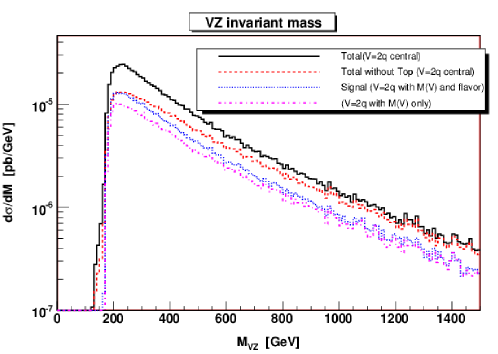
Figure 13.58: Invariant mass distribution of the lepton pair and the two jets from boson decay for the no-Higgs case. The solid(dashed) line is obtained identifying the two most central jets as the vector boson decay products before(after) top vetoing. The dotted line is obtained requiring the correct flavour content for the jets identified as decay products of both the vector boson and the top. The dot–dashed lines is produced using solely invariant mass informations to identify the vector boson and the top decay products.

It is not possible to separate the contribution of the various subprocesses ($ZW\rightarrow ZW$, $WW\rightarrow ZZ$, $ZZ\rightarrow ZZ$, $t\bar{t}$, single $t$) to a given six-fermion final state. Still, it is possible to isolate different subgroups of reactions including different subsets of diagrams. For example, only the subprocess $ZZ\rightarrow ZZ$ can be identified inside the scattering set of the diagrams describing the reaction $uu\rightarrow uus\bar{s}\mu^{+}\mu^{-}$, hence the latter will be unambigously assigned to the $ZZ\rightarrow ZZ$ subgroup. If more than one subprocess contributes to a given reaction, the same will appear in different subgroups. This is the case, for instance, with $ud\rightarrow uds\bar{s}\mu^{+}\mu^{-}$ ($ZZ\rightarrow ZZ$, $WW\rightarrow ZZ$). The plot on the left in Fig.13.59 shows the invariant mass distribution of the two most central quarks and of the two leptons for all reactions which contain the different subprocesses as well as the distribution for the complete set of processes. A light Higgs with $M_{H}=150$ GeV has been assumed. In order to comply with typical acceptance and trigger requirements, the standard acceptance cuts in Tab.13.17 have been applied. It should be clear that the total cross section in Fig.13.59 is smaller than the sum of the cross sections for the various groups as a consequence of double counting.

Acceptance cuts	Selection cuts
$p_{T}(\ell^{\pm})>20$ GeV	$|M(bW)-M_{top}|>15$ GeV
$|\eta(\ell^{\pm})|<3$	$|M(\ell^{+}\ell^{-})-M_{Z}|<10$ GeV
$E(q)>30$ GeV	$|M(q_{1}q_{2}\mbox{ from W})-M_{W}|<10$ GeV
$p_{T}(q)>20$ GeV	$|M(q_{1}q_{2}\mbox{ from Z})-M_{Z}|<10$ GeV
$|\eta(q)|<5$	$|M(q_{3}q_{4})-M_{W}|>10$ GeV
$M(\ell^{+}\ell^{-})>20$ GeV	$|M(q_{3}q_{4})-M_{Z}|>10$ GeV
$M(qq)>60$ GeV
$|\Delta\eta(\mbox{tag-quarks})|>3.8$

Table 13.17: Standard acceptance and selection cuts applied in results on the $\mu^{+}\mu^{-}$ channel. $M(q_{1}q_{2}\mbox{ from W(Z)})$ is the invariant mass of the two quarks with the correct flavour content to be produced in a $W(Z)$ decay. If more than one combination of two quarks satisfies this requirement, the one closest to the corresponding central mass value is selected. $M(q_{3}q_{4})$ denotes the invariant mass of the two remaining quarks.

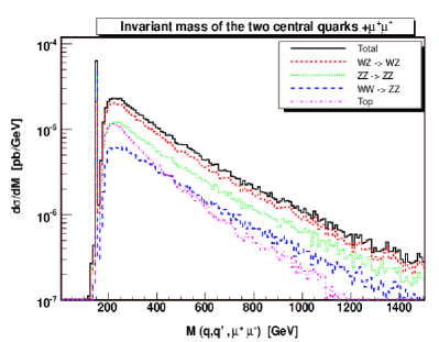
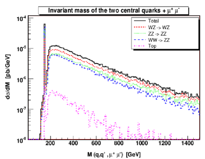
Figure 13.59: Invariant mass distribution of the two charged leptons and the two most central quarks, for different sets of processes. The plot on the left includes the set of acceptance cuts described in the left part of Tab.13.17. In the plot on the right a further cut for vetoing top production is applied.

For the selected type of final states, top background enters only through single $t$ production. Top candidates are rejected requiring a $b\>(\bar{b})$ quark in the final state together with two other quarks of the right flavour combination to be associated to a $W^{+}\>(W^{-})$ decay, with an invariant mass $M(bW)$ between 160 and 190 GeV. The plot on the right in Fig.13.59 shows the results after top subtraction. The subprocess $ZW\rightarrow ZW$ provides the most relevant contribution.

We intend to investigate the differences between the Standard Model and alternative scenarios in the high invariant mass region. In this analysis we have considered the Standard Model without Higgs sector, hereafter denoted no-Higgs scenario, which acts as an upper limit for new physics effects in models like those mentioned in Ref.[4]. Despite longitudinally polarized gauge bosons become strongly interacting in absence of the Higgs particle, detecting any deviation still remains a challenge at LHC because the rise of the cross section is masked by the decrease of parton luminosities at high energies. An analysis of selection cuts capable to enhance the difference between the no-Higgs and light-Higgs case could provide some guidance in the search for signals of new physics. As shown in Fig.13.60, simple requirements of centrality of the final-state bosons achieve this result at $\mathcal{O}(\alpha_{\scriptscriptstyle EM}^{6})$.

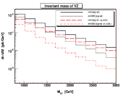
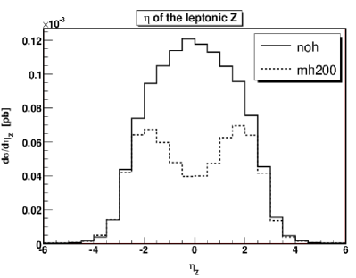
Figure 13.60: On the left: invariant mass distribution for $M(VZ)>800$ GeV. The full and long–dashed line refer to the no-Higgs case, the short–dashed and dot–dashed ones to $M_{H}=200$ GeV. All results satisfy the standard acceptance and selection cuts reported in Tab.13.17. For the long–dashed and dot–dashed histograms we have further required $|\eta(\ell^{+}\ell^{-})|<\$2 and $|\eta(qq\mbox{ from }V)|<\$2. On the right: pseudorapidity distribution of the $Z$ reconstructed from leptons.

The procedure we adopted for separating jets imposes a minimum invariant mass of 60 GeV for each pair of quarks. An alternative approach consists in requiring a minimum $\Delta R$ separation among coloured particles and is discussed in Tab.13.18. We find out that the no-Higgs case is more sensitive than light-Higgs to cuts based on $\Delta R$. Indeed, in the model without Higgs the outgoing vector bosons are favoured to be more central and they have a larger $p_{T}$. As a consequence of Lorentz boost they decay producing two quarks with small relative angle which are most likely to merge into one jet unless a sufficiently small $\Delta R$ is selected. The larger is the minimum separation required, the smaller the number of expected events. This is an indication that low $\Delta R$ cuts should be studied to evidentiate new physics.

On the other hand, alternative procedures for jet reconstruction based on the $K_{\perp}$ algorithm have been recently proposed[14], which may prove useful in connection with this kind of studies as they lead to encouraging results in identifying hadronic decays of heavy bosons via a cut on the sub-jet separation scale.

$M_{cut}$	no Higgs		$M_{H}=200$ GeV		Ratio
800 GeV	31	(14,17)	12	(7,5)	2.59
900 GeV	25	(12,13)	8	(5,3)	3.12
1.0 TeV	19	(9,10)	6	(4,2)	3.16
$\Delta R=0.4$
$M_{cut}$	no Higgs		$M_{H}=200$ GeV		Ratio
800 GeV	18	(8,10)	10	(6,4)	1.80
900 GeV	12	(5,7)	6	(4,2)	2.00
1.0 TeV	8	(4,4)	4	(2,2)	2.00
$\Delta R=0.5$
$M_{cut}$	no Higgs		$M_{H}=200$ GeV		Ratio
800 GeV	12	(5,7)	8	(5,3)	1.50
900 GeV	8	(4,4)	5	(4,2)	1.60
1.0 TeV	5	(2,3)	3	(2,1)	1.60

Table 13.18: Number of events as a function of the minimum invariant mass of the $ZV\rightarrow\mu^{+}\mu^{-}jj$ pair for $\mathcal{L}=100\;\mbox{fb}^{-1}$, having applied the cuts in Tab.13.17[15]. All events satisfy $|\eta(\ell^{+}\ell^{-})|<2$ and $|\eta(qq\mbox{ from }V)|<2$. In brackets we show the contribution of the ($ZW$, $ZZ$) final states.

13.51 $\mathcal{O}(\alpha_{\scriptscriptstyle EM}^{6})+\mathcal{O}(\alpha_{\scriptscriptstyle EM}^{4}\alpha_{\scriptscriptstyle S}^{2})$ results in the semileptonic $\mu\nu_{\mu}$ channel

We will now investigate how much the sensitivity to the $VV$ scattering signal is affected by the QCD irreducible background, which is expected to considerably dilute the differences between the light-Higgs and no-Higgs scenarios evidentiated in the previous section. To this purpose, we consider the full set of parton-level processes involved at $\mathcal{O}(\alpha_{\scriptscriptstyle EM}^{6})+\mathcal{O}(\alpha_{\scriptscriptstyle EM}^{4}\alpha_{\scriptscriptstyle S}^{2})$,

$$qq\rightarrow qqqq\mu\bar{\nu}_{\mu}\hskip 22.76228ptgg\rightarrow qqqq\mu\bar{\nu}_{\mu}$$

$$gq\rightarrow gqqq\mu\bar{\nu}_{\mu}\hskip 22.76228ptqq\rightarrow ggqq\mu\bar{\nu}_{\mu}$$ ,

together with a selection procedure as close as possible to the actual experimental practice, without resorting to any flavour information other than the one which a typical $b$-tagging algorithm is able to provide. The $p_{Z}$ of the neutrino is approximately reconstructed by imposing the invariant mass of the two leptons equal to the $W$ boson nominal mass:

$$(p^{\mu}+p^{\nu})^{2}=M_{W}^{2}.$$ (13.40)

This equation has two solutions,

$$p_{z}^{\nu}={\alpha p_{z}^{\mu}\pm\sqrt{\alpha^{2}p_{z}^{\mu 2}-(E^{\mu 2}-p_{z}^{\mu 2})(E^{\mu 2}p_{T}^{\nu 2}-\alpha^{2})}\over E^{\mu 2}-p_{z}^{\mu 2}}\;,$$ (13.41)

where

$$\alpha={M_{W}^{2}\over 2}+p_{x}^{\mu}p_{x}^{\nu}+p_{y}^{\mu}p_{y}^{\nu}\;.$$ (13.42)

The event is rejected if the discriminant of Eq.(13.41) is negative, otherwise both the solutions are required to pass the selection cuts.

All the results presented in this section have been obtained using the CTEQ5L PDF set and the QCD coupling constant running at the scale

$$Q^{2}=M_{top}^{2}+p_{T}(top)^{2},$$ (13.43)

where $p_{T}(top)$ is the transverse momentum of the reconstructed top, for all processes in which a $t$ or $\bar{t}$ can be produced. For all the other processes the scale has been evaluated as in Eq.(13.39).

$M_{H}=200$ GeV	$\sigma_{\scriptscriptstyle{{EW}}}$	$\sigma_{\scriptscriptstyle{EW+QCD}}$
all events	0.89 pb	80.8 pb
top events	0.52 pb	71.6 pb
ratio top/all	0.58	0.89

Table 13.19: Contribution of $t\bar{t}$/single $t$ to the total cross section with standard acceptance cuts only (see the left part of Tab.13.20). Comparison between results at $\mathcal{O}(\alpha_{\scriptscriptstyle EM}^{6})$ (EW) and $\mathcal{O}(\alpha_{\scriptscriptstyle EM}^{6})+\mathcal{O}(\alpha_{\scriptscriptstyle EM}^{4}\alpha_{\scriptscriptstyle S}^{2})$ (EW+QCD). Interferences between the two perturbative orders are neglected.

It should be clear from the results shown in Tab.13.19 that suppressing the top background is the primary objective to achieve. In this analysis we assume the possibility to tag $b$-jets in the central region with 0.8 efficiency for $|\eta|<1.5$, which allows to discard part of the events containing $b$ quarks in the final state. We impose additional cuts against top on the invariant mass of triplets of type $\{jjj\}$ and $\{j\mu\nu\}$, where $j$ denotes any final-state quark or gluon. In order to isolate two vector boson production, kinematical cuts are applied on the invariant mass of the two most central jets, which are associated in our analysis to a $W$ or $Z$ decaying hadronically. The $VV$ fusion signature is further isolated by requiring a minimum $\Delta\eta$ separation between the two forward/backward jets.

At this stage, however, any attempt to appreciate differences between Higgs and no-Higgs scenarios at high invariant masses would still be vain. This is essentially due to the fact that the contribution of the QCD diagrams depicted in Fig.13.57(c,d) is not substantially affected by the above-mentioned selection criteria. Investigating the differences between the kinematics of $VV$ scattering and $VV+2\,jets$, we have identified additional cuts that serve our purpose. As the background dominates in the phase space regions characterized by one vector boson and the forward/backward jet produced with small invariant mass, a viable method of taming $VV+2\,jets$ consists in applying cuts on the $p_{T}$ and $\eta$ of the $W$ reconstructed from leptons as well as on the invariant mass of the $W$ plus one of the two tag jets. All details about the selection cuts applied are reported in Tab.13.20.

Acceptance cuts	Selection cuts
$p_{T}(\ell^{\pm},j)>10$ GeV	$b$-tagging for $|\eta|<1.5$ (80% efficiency)
$E(\ell^{\pm},j)>20$ GeV	$|M(jjj;j\ell^{\pm}\nu_{rec})-M_{top}|>15$ GeV
$|\eta(\ell^{\pm})|<3$	$70\mbox{GeV}<M(j_{c}j_{c})<100$ GeV
$|\eta(j)|<6.5$	$M(j_{f}j_{b})<70$ GeV ; $M(j_{f}j_{b})>100$ GeV
	$M(jj)>60$ GeV
	$\Delta\eta(j_{f}j_{b})>4$
	$p_{T}(\ell^{\pm}\nu_{rec})>100$ GeV
	$\eta(\ell^{\pm}\nu_{rec})<2$
	$M(j_{f/b}\ell^{\pm}\nu_{rec})>250$ GeV

Table 13.20: List of kinematical cuts applied in all results on the $\mu\nu_{\mu}$ channel. $j$ denotes any final-state quark or gluon, while $\ell^{\pm}$ is the charged lepton. The subfixes $c$,$f$,$b$ mean central, forward, backward respectively. $\nu_{rec}$ is the neutrino reconstructed following the prescription of Eq.(13.40)

$\mathcal{O}(\alpha_{\scriptscriptstyle EM}^{6})$	no Higgs		$M_{H}=200$ GeV
	$\sigma$	$\mathcal{L}$=$100\,\mbox{fb}^{-1}$	$\sigma$	$\mathcal{L}$=$100\,\mbox{fb}^{-1}$	ratio
all events	12.46 fb	1246 $\pm$ 35	13.57 fb	1357 $\pm$ 37	0.918
$M_{cut}=0.8$ TeV	3.19 fb	319 $\pm$ 18	1.45 fb	145 $\pm$ 12	2.200
$M_{cut}=1.2$ TeV	1.28 fb	128 $\pm$ 11	0.41 fb	41 $\pm$ 6	3.122
$M_{cut}=1.6$ TeV	0.60 fb	60 $\pm$ 8	0.14 fb	14 $\pm$ 4	4.286

Table 13.21: Integrated $\mathcal{O}(\alpha_{\scriptscriptstyle EM}^{6})$ cross section for $M(j_{c}j_{c}l\nu)>M_{cut}$ and number of expected events after one year at high luminosity having applied the cuts listed in Tab.13.20.

$\mathcal{O}(\alpha_{\scriptscriptstyle EM}^{6})\;+$	no Higgs		$M_{H}=200$ GeV
$\mathcal{O}(\alpha_{\scriptscriptstyle EM}^{4}\alpha_{\scriptscriptstyle S}^{2})$	$\sigma$	$\mathcal{L}$=$100\,\mbox{ fb}^{-1}$	$\sigma$	$\mathcal{L}$=$100\,\mbox{ fb}^{-1}$	ratio
all events	40.70 fb	4070 $\pm$ 64	40.73 fb	4073 $\pm$ 64	0.999
$M_{cut}=0.8$ TeV	7.61 fb	761 $\pm$ 28	5.14 fb	514 $\pm$ 23	1.481
$M_{cut}=1.2$ TeV	2.53 fb	253 $\pm$ 16	1.73 fb	173 $\pm$ 13	1.462
$M_{cut}=1.6$ TeV	1.00 fb	100 $\pm$ 10	0.55 fb	55 $\pm$ 7	1.818

Table 13.22: Integrated $\mathcal{O}(\alpha_{\scriptscriptstyle EM}^{6})+\mathcal{O}(\alpha_{\scriptscriptstyle EM}^{4}\alpha_{\scriptscriptstyle S}^{2})$ cross section for $M(j_{c}j_{c}l\nu)>M_{cut}$ and number of expected events after one year at high luminosity having applied the cuts listed in Tab.13.20. Interferences between the two perturbative orders are neglected.

Fig.13.61,13.62 illustrate the final results of our analysis, showing that the top background is basically under control. $VV+2\,jets$ still provides a non-negligible contribution over the whole invariant mass spectrum, nevertheless differences between light-Higgs and no-Higgs can be appreciated. In Tab.13.21,13.22 we show the integrated cross section at high energies as a function of the minimum invariant mass, comparing results of the pure EW and EW+QCD cases. Despite reducing the ratio between no-Higgs and light-Higgs cross sections, the inclusion of QCD background seems not to compromise the possibility of finding signals of EWSB at LHC. We find that about 500 events are expected above 800 GeV after one year of high luminosity running ($\mathcal{L}=100\mbox{ fb}^{-1}$) in case of a Higgs boson with mass 200 GeV. The Higgsless model predicts about 250 more events in accordance with the enhancement of the $VV$ differential cross section at high energies. These numbers refer to the muon channel only, and are obviously improved by summing up the muon and electron channels. It should nevertheless be noticed that imposing a minimum $\Delta R$ separation among coloured particles could degrade these preliminary results and requires further investigations.

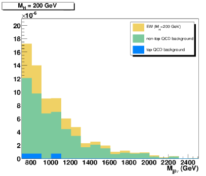
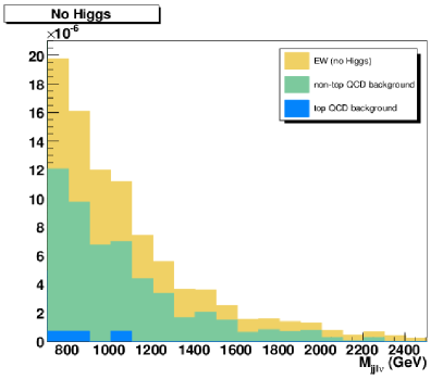
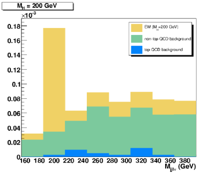
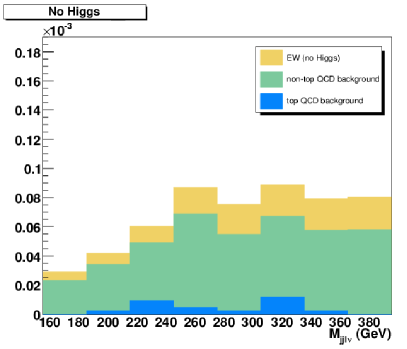
Figure 13.61: Invariant mass distribution of the two leptons and the two most central jets in the Standard Model with a light Higgs (on the left) and in the no-Higgs scenario (on the right). The cuts applied are listed in Tab.13.20. $\mathcal{O}(\alpha_{\scriptscriptstyle EM}^{6})$ (EW) and $\mathcal{O}(\alpha_{\scriptscriptstyle EM}^{4}\alpha_{\scriptscriptstyle S}^{2})$ (QCD) contributions to the differential cross section have been isolated and are shown separately. The QCD contributions are further split into top background (in blue) and $VV+2\,jets$ (in green).

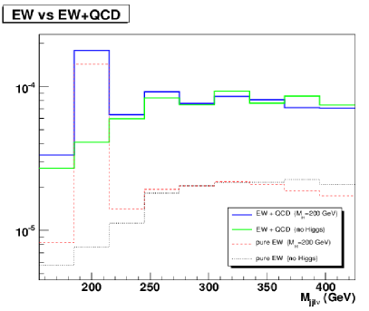
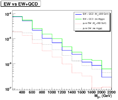
Figure 13.62: Invariant-mass distribution of the two leptons plus the two most central jets in the pure EW ($\mathcal{O}(\alpha_{\scriptscriptstyle EM}^{6})$) and EW+QCD ($\mathcal{O}(\alpha_{\scriptscriptstyle EM}^{6})+\mathcal{O}(\alpha_{\scriptscriptstyle EM}^{4}\alpha_{\scriptscriptstyle S}^{2})$) case. Comparison between light-Higgs ($M_{H}=200$ GeV) and no-Higgs results. Interferences between the two different perturbative orders are neglected. The cuts applied are listed in Tab.13.20

13.52 Conclusions

The results presented in this note should be intended as the starting point of a larger complete study which aims at providing an up-to-date and hopefully more reliable answer on the sensitivity of Boson-Boson Scattering as a probe of the symmetry breaking mechanism at LHC. In spite of theoretical uncertaintes tipically estimated of $\mathcal{O}(10)$%, these results put a benchmark at parton level to the possibility of extracting the $VV$ scattering signal from its irreducible background. There are clear indications that, with a complete calculation and appropriate kinematical cuts, the Higgs and no-Higgs cases show appreciable differences even after including the most relevant QCD contributions. We find in our analysis that the number of events expected in the Higgsless scenario is about 50% larger than the one predicted by the Standard Model with a 200 GeV Higgs boson. More refined selection criteria are under study in order to enhance further the Higgs signal as well as any possible deviation from the Standard Model expectations in the high invariant mass region. As an evolution for the near future, the analysis will be extended to cover $V+4\,jets$ contributions so that a full estimate of the QCD background in the semileptonic channel will be available.

Searching for Extra Neutral Interactions at the LHC

Roberta Armillis, Claudio Corianò, Alon E. Faraggi, Marco Guzzi, Nikos Irges

Abstract

We present a brief overview of some aspects of the theory and phenomenology of models containing extra neutral currents in abelian extensions of the Standard Model. We illustrate the mechanism of anomaly cancellation as a way to infer the charge assignments of the fermion spectrum and then briefly discuss a variant of this approach where an effective action is rendered anomaly-free by a mechanism involving an axion via a Wess-Zumino term. Measurements at the LHC on the Z resonance in leptoproduction will be able to exclude a class of these models for variations of the cross section at the level of $4\%$, which is obtained at larger values of the anomalous coupling $(g_{z}\approx 1)$. The anomalous nature is unlikely to be resolved with an inclusive NNLO analysis.

14.53 Introduction

The search for extra abelian gauge interactions will surely be an important component of the experimental program at the LHC. In fact, extra neutral interactions, or “extra $Z^{\prime}$”, as they are commonly known, are predicted by several theoretical constructions such as Grand Unified Theories, Superstring Theory, and, more recently, by a class of models characterized by intersecting branes, just to mention a few (see [1], [2],[3]). One of the most relevant channels useful for the search of extra neutral currents is lepton pair production, at an invariant mass of the lepton pair not too large compared to the Z mass, since the invariant mass distribution $d\sigma/dM^{2}$ is rapidly falling, so to allow to gather enough statistics and separate the signal from the Standard Model background. Being the mass of the extra gauge boson (or bosons) undetermined, as is the coupling constant of the extra neutral current, a scan of the entire high energy tail of the Drell-Yan distribution is required. The width of these resonances is also undetermined by the theoretical models and may change considerably depending on the underlying assumptions of each theoretical construction. We will summarize below some of the main motivations of these searches discussing both anomaly-free models and a class of models where the anomaly is cancelled via the inclusion of a pseudoscalar, the Axi-Higgs [5], which is part of the Higgs sector. In models of this type the phenomenology of the extra $Z^{\prime}$ shows some very distinctive features at the level of trilinear gauge interactions. A more detailed analysis of the topics addressed in this contribution can be found in [6, 7, 8, 9, 10, 11, 12]. The numerical study that we present is performed on the abelian extension of [13], whose analysis is extended here, in part, to next-to-next-to-leading order in QCD. Other recent analysis addressing a general family-blind $U(1)$ is in [14] and briefly highlighted in the next section. A more detailed analysis of some of the issues addressed here are presented in [10].

14.54 Non Anomalous $U(1)$’s

The interaction of an extra neutral gauge boson $U(1)$ with the fermions of the Standard Model requires a suitable definition of their charges with respect to the new additional neutral interactions. Some of the most useful and powerful constraints in fixing the charges of these models is the requirement that they are free of anomalies. We will bring in a simple example to illustrate how the cancellation works for the case of one extra gauge factor, $U(1)_{z}$, assuming a chiral spectrum that includes also a set of extra fermions $\nu_{k}$, with $k=1,2,...,n$ indicating a certain number of right-handed neutrinos. For simplicity we will assume that the interaction is family universal, which means that the cancellations take place generation by generation. We consider a model with the gauge symmetry $SU(3)\times SU(2)\times U(1)\times U(1)_{z}$. Breaking the gauge symmetry down to $SU(3)\times U(1)_{em}$ requires an extra scalar sector compared to the SM. This can be achieved in different ways, for instance by including, beside the Higgs doublet, a $SU(2)_{W}$ singlet $\phi$, whose vacuum expectation value is $v_{\phi}$. In a more general framework, the constraints on the interactions of the $U(1)_{z}$ gauge boson with the fermions of the SM are relaxed if two Higgs doublets, $H_{1}$ and $H_{2}$, together with an extra scalar $\phi$, are introduced (see [13]).

14.55 Phenomenological Models: An Example

Following [14] we consider three generations of quarks, $q_{L}^{i},u_{R}^{i},d_{R}^{i}$, and leptons, $l_{L}^{i},e_{R}^{i}$, $i=1,2,3$, and a number $n$ of right-handed neutrinos, $\nu_{R}^{k}$, $k=1,...,n$, which are singlets under $SU(3)_{C}\times SU(2)_{W}$. We label the $U(1)_{z}$ charges as $z_{q},z_{u},z_{d},z_{l},z_{e}$, for the standard model fermions, and $z_{k}$ are the charges of the right-handed neutrinos. The Higgs sector of the Standard Model is enlarged with an extra singlet $\phi$, as shown in Table 1. $H$ is the electroweak Higgs. The cancellation of the anomalous interactions, for instance those involving the $[SU(2)_{W}]^{2}U(1)_{z}$ and $[SU(3)_{C}]^{2}U(1)_{z}$ gauge currents requires that

$$z_{l}=-3z_{q}$$

$$z_{d}=2z_{q}-z_{u}.$$ (14.44)

Similarly, the $[U(1)_{Y}]^{2}U(1)_{z}$ anomaly cancellation then implies that

$$z_{e}=-2z_{q}-z_{u}.$$ (14.45)

Eqs. (14.44) and (14.45) together lead to the conclusion that only two independent real parameters, $z_{q}$ and $z_{u}$, describe the allowed $U(1)_{z}$ charges of the quarks and $U(1)_{Y}$-charged leptons. Equivalently, the $U(1)_{z}$ charges may be expressed as a linear combination of $Y$ and $B-L$: $(z_{u}-z_{q})Y+(4z_{q}-z_{u})(B-L)$.

	$SU(3)_{C}$	$SU(2)_{W}$	$U(1)_{Y}$	$U(1)_{z}$
$q_{L}^{i}$	3	2	$1/3$	$z_{q}$
$u_{R}^{i}$	3	1	$4/3$	$z_{u}$
$d_{R}^{i}$	3	1	$-2/3$	$2z_{q}-z_{u}$
$l_{L}^{i}$	1	2	$-1$	$-3z_{q}$
$e_{R}^{i}$	1	1	$-2$	$-2z_{q}-z_{u}$
$\nu_{R}^{k}$ , $k=1,...,n$	1	1	0	$z_{k}$
$H$	1	2	$+1$	$-z_{q}+z_{u}$
$\varphi$	1	1	$0$	$1$

Table 14.23: Charge assignement for the Appelquist model

Additional restrictions on the $U(1)_{z}$ charges are imposed by the mixed gravitational-$U(1)_{z}$ and $[U(1)_{z}]^{3}$ anomaly cancellation conditions

$${1\over 3}\sum_{k=1}^{n}z_{k}=-4z_{q}+z_{u}~{},$$ (14.46)

$$\left(\sum_{k=1}^{n}z_{k}\right)^{\!3}=9\sum_{k=1}^{n}z_{k}^{3}~{}.$$ (14.47)

For $n=1$ or $2$, the charge assignments compatible with these equations constrain $U(1)_{z}$ to be proportional to the hypercharge, giving a solution termed “sequential”, while more general solutions can be found already for $n=3$, which can be expressed in terms of a free parameter. The analysis of the possible neutrino mass terms compatible with a given charge assignment can also be used as a way to select the most interesting solutions of these equations. For instance, in the case $n=3$ both Dirac and Majorana mass terms are possible in this minimal model (see [14] for more details). It is understood that a modification of the Higgs sector renders the study more involved [13].

14.56 Heterotic–string inspired $Z^{\prime}$

The heterotic–string gives rise to effective field theories that descend from the $E_{8}\times E_{8}$ or $SO(32)$ groups of the ten dimensional theories. The first case gives rise to additional $Z^{\prime}$s that arise in the $SO(10)$ and $E_{6}$ extensions of the Standard Model. A basis for the extra $Z^{\prime}$ arising in these models is formed by the two groups $U(1)_{\chi}$ and $U(1)_{\psi}$ via the decomposition $E_{6}\rightarrow SO(10)\times U(1)_{\psi}$ and $SO(10)\rightarrow SU(5)\times U(1)_{\chi}$ [2]. Additional, flavor non–universal $U(1)$’s, may arise in heterotic $E_{8}\times E_{8}$ string models from the $U(1)$ currents in the Cartan subalgebra of the four dimensional gauge group, that are external to $E_{6}$. Non–universal $Z^{\prime}$s typically must be beyond the LHC reach, to avoid conflict with Flavor Changing Neutral Currents (FCNC) constraints. Recently [6] a novel $Z^{\prime}$ in quasi–realistic string models that do not descend from the $E_{8}\times E_{8}$ has been identified. Under the new $U(1)$ symmetry left–handed components and right–handed components in the 16 spinorial $SO(10)$ representation, of each Standard Model generation, have charge $-1/2$ and $+1/2$, respectively. As a consequence, the extra $U(1)$ is family universal and anomaly free. It arises in left-right symmetric string models, in which the $SO(10)$ symmetry is broken directly at the string level to $SU(3)\times U(1)_{B-L}\times SU(2)_{L}\times SU(2)_{R}\times U(1)_{Z^{\prime}}\times U(1)^{n}\times{\rm hidden}$ [15]. The $U(1)^{n}$ are flavor dependent $U(1)$s that are broken near the string scale. The Standard Model matter states are neutral under the hidden sector gauge group, which in these string models is typically a rank eight group. It is important to note that the fact that the spectrum is derived from a string vacuum that satisfies the modular invariance constraints, establishes that the model is free from gauge and gravitational anomalies. The pattern of $U(1)_{Z^{\prime}}$ charges in the quasi–realistic string models of ref. [15] does not arise in related string models in which the $SO(10)$ symmetry is broken to a different subgroup.

The important function of this $Z^{\prime}$ is that it forbids dimension four, five and six proton decay mediating operators [16]. The extra $U(1)$ is anomaly free and family universal. It allows the fermions Yukawa couplings to the Higgs field and the generation of small neutrino masses via a seesaw mechanism. The existence of an extra $Z^{\prime}$ at low energies is motivated by proton longevity, and the suppression of the proton decay mediating operators. String models contain several $U(1)$ symmetries that suppress the proton decay mediating operators. However, these are typically non–family universal. They constrain the fermion mass terms and hence must be broken at a high scale. Thus, the existence of a $U(1)$ symmetry that can remain unbroken down to low energies is highly nontrivial. The $U(1)$ symmetry in ref. [15, 6] satisfies all of these requirements. Furthermore, as the generation of small neutrino masses in the string models arises from the breaking of the $B-L$ current, the extra $U(1)$ allows lepton number violating terms, but forbids the baryon number violating terms. Hence, it predicts that $R$–parity is violated and its phenomenological implications for SUSY collider searches differ substantially from models in which $R$–parity is preserved.

14.57 Anomalous $U(1)^{\prime}s$: Cancelling the anomalies via higher dimensional operators

The simplest effective theory that allows a cancellation of the gauge anomalies includes a Wess-Zumino term with a shifting axion. The role of the axion has been a matter of debate in the past [17], since with a suitable gauge choice one can set the axion to vanish. Undoubtly, the axion can also be interpreted as the phase of an additional (second) Higgs when either large Yukawa couplings or a large vev of this additional Higgs is responsible for the decoupling of one or more chiral fermions [7]. According to this picture, an effective anomalous theory is then the result of the partial decoupling of part of the fermion spectrum, leaving the left-over fermions in a reducible representation. The induced Wess-Zumino term is of the form $b/M_{1}F\wedge F$, a dimension-5 operator, where $b$ is an axion and $F$ is the field strength of a gauge interaction. The $1/M_{1}$ suppression of the axion-gauge interaction is directly related to the vev of the Higgs and $b$ is its pseudoscalar phase [7]. The scale $M_{1}$ is completely unrelated to the mechanism held responsible for the generation of a mass for the axion and remains a free parameter (see [18]). The mechanism of partial decoupling is a generic feature of effective anomalous theories that brings into the effective action a gauged axion.

In general, models based on intersecting branes predict similar structures, though the axion of the effective theory is not a consequence of partial decoupling. The Standard Model, in this case, is enlarged with several extra anomalous $U(1)$’s, one combination of which is anomaly free and is identified with the hypercharge, while the remaining U(1)’s are accompanied by axions. These models predict a single physical axion (the Axi-Higgs) [5] and contain generalized Chern-Simons terms in the effective action [5], [19], [7]. These terms are necessary in order to render the abelian interactions anomaly-free. On the contrary of non-anomalous $U(1)$ models, which have similar properties and difficult to discern at the LHC, anomalous U(1)’s show some interesting features both in Drell-Yan at NNLO [12], due to non-cancelling anomalous contribution and to the possibility of an axion exchange. We refer to [7, 8] for a discussion of the detection of modified trilinear interaction in the neutral sector ( $Z\,\gamma\,\gamma$ vertex).

14.58 The detection of extra $Z$-primes at the LHC

We quantify below the rates for the invariant mass distributions in the case of the model of [13]. The approach follows closely [20, 21, 22]. Our convention for the couplings of the ${\cal Z}=Z,Z^{\prime}$ to the quarks and leptons are written below

$${g_{V}}^{Z,j}=2\left[c_{w}^{2}(T_{3}^{L,j}+T_{3}^{R,j})-s_{w}^{2}({\hat{Y}^{j}_{L}\over 2}+{\hat{Y}^{j}_{R}\over 2})+\varepsilon{g_{z}\over g}c_{w}({\hat{z}_{L,j}\over 2}+{\hat{z}_{R,j}\over 2})\right]$$

$${g_{A}}^{Z,j}=2\left[c_{w}^{2}(T_{3}^{R,j}-T_{3}^{L,j})-s_{w}^{2}({\hat{Y}^{j}_{R}\over 2}-{\hat{Y}^{j}_{L}\over 2})+\varepsilon{g_{z}\over g}c_{w}({\hat{z}_{R,j}\over 2}-{\hat{z}_{L,j}\over 2})\right]$$

$${g_{V}}^{Z^{\prime},j}=2\left[-\varepsilon c_{w}^{2}(T_{3}^{L,j}+T_{3}^{R,j})+\varepsilon s_{w}^{2}({\hat{Y}^{j}_{L}\over 2}+{\hat{Y}^{j}_{R}\over 2})+{g_{z}\over g}c_{w}({\hat{z}_{L,j}\over 2}+{\hat{z}_{R,j}\over 2})\right]$$

$${g_{A}}^{Z^{\prime},j}=2\left[-\varepsilon c_{w}^{2}(T_{3}^{R,j}-T_{3}^{L,j})+\varepsilon s_{w}^{2}({\hat{Y}^{j}_{R}\over 2}-{\hat{Y}^{j}_{L}\over 2})+{g_{z}\over g}c_{w}({\hat{z}_{R,j}\over 2}-{\hat{z}_{L,j}\over 2})\right]$$

where $j$ is an index that runs over the quarks and the lepton, and $\sin\theta_{W}=s_{w},\cos\theta_{W}=c_{w}$ for brevity. The mixing in the neutral sector appears through the parameter $\varepsilon$, defined as

$$\varepsilon={\delta M^{2}_{ZZ^{\prime}}\over M^{2}_{Z^{\prime}}-M^{2}_{Z}}$$

$$M_{Z}^{2}={g^{2}\over 4\cos^{2}\theta_{W}}(v_{H_{1}}^{2}+v_{H_{2}}^{2})\left[1+O(\varepsilon^{2})\right]$$

$$M_{Z^{\prime}}^{2}={g_{z}^{2}\over 4}(z_{H_{1}}^{2}v_{H_{1}}^{2}+z_{H_{2}}^{2}v_{H_{2}}^{2}+z_{\phi}^{2}v_{\phi}^{2})\left[1+O(\varepsilon^{2})\right]$$

$$\delta M^{2}_{ZZ^{\prime}}=-{gg_{z}\over 4\cos\theta_{W}}(z_{H_{1}}^{2}v_{H_{1}}^{2}+z_{H_{2}}^{2}v_{H_{2}}^{2}),\,$$ (14.49)

where we have chosen [13] $z_{H_{1}}=z_{H_{2}}=0$, $v_{H_{2}}=246$ GeV and $\tan{\beta}=1$ and have defined $g={e}/{\sin\theta_{W}},g_{Y}={e}/{\cos\theta_{W}}$. Precision studies at LEP constrain $\varepsilon$ to be smaller than $10^{-3}$.

The decay rates into leptons for the $Z$ and the $Z^{\prime}$ are universal and are given by

$$\Gamma({\cal Z}\rightarrow l\bar{l})={g^{2}\over 192\pi c_{w}^{2}}M_{{\cal Z}}\left[(g_{V}^{{\cal Z},l})^{2}+(g_{A}^{{\cal Z},l})^{2}\right]={\alpha_{em}\over 48s_{w}^{2}c_{w}^{2}}M_{{\cal Z}}\left[(g_{V}^{{\cal Z},l})^{2}+(g_{A}^{{\cal Z},l})^{2}\right]\,,$$

$$\Gamma({\cal Z}\rightarrow\psi_{i}\bar{\psi_{i}})={N_{c}\alpha_{em}\over 48s_{w}^{2}c_{w}^{2}}M_{{\cal Z}}\left[(g_{V}^{{\cal Z},\psi_{i}})^{2}+(g_{A}^{{\cal Z},\psi_{i}})^{2}\right]\times$$

$$\hskip 85.35826pt\left[1+{\alpha_{s}(M_{{\cal Z}})\over\pi}+1.409{\alpha_{s}^{2}(M_{{\cal Z}})\over\pi^{2}}-12.77{\alpha_{s}^{3}(M_{\cal Z})\over\pi^{3}}\right],\,$$ (14.50)

where $i=u,d,c,s$ and ${\cal Z}=Z,Z^{\prime}$. For the $Z^{\prime}$ and $Z$ decays into heavy quarks we have used (see Ref.[23, 24])

$$\Gamma({\cal Z}\rightarrow b\bar{b})={N_{c}\alpha_{em}\over 48s_{w}^{2}c_{w}^{2}}M_{{\cal Z}}\left\{(g_{V}^{{\cal Z},b})^{2}\left[c_{0}+c_{1}{\alpha_{s}(M_{\cal Z})\over\pi}+\dots\right]+(g_{A}^{{\cal Z},b})^{2}\left[d_{0}+d_{1}{\alpha_{s}(M_{\cal Z})\over\pi}+\dots\right]\right\},$$

$$\Gamma({\cal Z}\rightarrow t\bar{t})={N_{c}\alpha_{em}\over 48s_{w}^{2}c_{w}^{2}}M_{{\cal Z}}\beta\left\{(g_{V}^{{\cal Z},t})^{2}{(3-\beta^{2})\over 2}A_{1}+(g_{A}^{{\cal Z},t})^{2}A_{2}\right\},$$ (14.51)

where the coefficients $c_{0},c_{1},d_{0},d_{1}$ are defined in Eq. (4.1) of [24] and where as in [23] we have defined

$$\beta=\sqrt{1-4{m_{t}^{2}\over M_{{\cal Z}}^{2}}},\hskip 28.45274ptA_{1}=\left\{1+{4\over 3}\alpha_{s}(M_{\cal Z})\left[{\pi\over 2\beta}-{3+\beta\over 4}\left({\pi\over 2}-{3\over 4\pi}\right)\right]\right\},$$

$$A_{2}=\left\{1+{4\over 3}\alpha_{s}(M_{\cal Z})\left[{\pi\over 2\beta}-\left({19\over 10}-{22\beta\over 5}+{7\beta^{2}\over 2}\right)\left({\pi\over 2}-{3\over 4\pi}\right)\right]\right\}.$$ (14.52)

Then, the total decay rate for the $Z$ and $Z^{\prime}$ is obtained by summing over each fermionic contribution, for instance

$$\Gamma_{Z^{\prime}}=\sum_{i=u,d,c,s}\Gamma(Z^{\prime}\rightarrow\psi_{i}\bar{\psi_{i}})+\Gamma(Z^{\prime}\rightarrow b\bar{b})+\Gamma(Z^{\prime}\rightarrow t\bar{t})+3\Gamma(Z^{\prime}\rightarrow l\bar{l})+3\Gamma(Z^{\prime}\rightarrow\nu_{l}\bar{\nu_{l}}).$$

14.58.1 Calculation of the point-like cross section in the $Z^{\prime}$ case

We come now briefly to discuss the quantification of the invariant mass distributions around the resonances in leptoproduction.

The colour-averaged inclusive differential cross section for the reaction $H_{1}+H_{2}\rightarrow l_{1}+l_{2}+X$, is given by [25]

$${d\sigma\over dQ^{2}}=\tau\sigma_{V}(Q^{2},M_{V}^{2})W_{V}(\tau,Q^{2})\hskip 28.45274pt\tau={Q^{2}\over S},$$ (14.54)

where $V$ refers to the generic vector bosons $Z,\gamma,Z^{\prime}$ and where all the hadronic initial state information is contained in the hadronic structure function which is defined as

$$W_{V}(\tau,Q^{2})=\sum_{i,j}\int_{0}^{1}dx_{1}\int_{0}^{1}dx_{2}\int_{0}^{1}dx\delta(\tau-xx_{1}x_{2})PD_{i,j}(x_{1},x_{2},\mu_{F}^{2})\Delta_{i,j}(x,Q^{2},\mu_{F}^{2})\,,$$

where the quantity $PD_{i,j}(x_{1},x_{2},\mu_{F}^{2})$ contains all the information about the parton distribution functions and their evolution to the $\mu_{F}^{2}$ scale and the $\Delta$’s are the flavour-dependent $(i,j)$ hard scatterings.

The point-like cross sections for the case of the $Z^{\prime}$ boson are given by

$$\sigma_{{Z^{\prime}}}(Q^{2})={\pi\alpha_{em}\over 4M_{{Z^{\prime}}}\sin^{2}\theta_{W}\cos^{2}\theta_{W}N_{c}}{\Gamma_{{Z^{\prime}}\rightarrow\bar{l}l}\over(Q^{2}-M_{Z^{\prime}}^{2})^{2}+M_{Z^{\prime}}^{2}\Gamma_{Z^{\prime}}^{2}}$$

$$\sigma_{{Z^{\prime}},\gamma}(Q^{2})={\pi\alpha_{em}^{2}\over 6N_{c}}{g_{V}^{Z^{\prime},l}g_{V}^{\gamma,l}\over\sin^{2}{\theta_{W}}\cos^{2}{\theta_{W}}}{(Q^{2}-M_{Z^{\prime}}^{2})\over Q^{2}(Q^{2}-M_{Z^{\prime}}^{2})^{2}+M_{Z^{\prime}}^{2}\Gamma_{Z^{\prime}}^{2}},$$

$$\sigma_{{Z^{\prime}},Z}(Q^{2})={\pi\alpha_{em}^{2}\over 96}{\left[g_{V}^{Z^{\prime},l}g_{V}^{Z,l}+g_{A}^{Z^{\prime},l}g_{A}^{Z,l}\right]\over\sin^{4}{\theta_{W}}\cos^{4}{\theta_{W}}N_{c}}$$

$$\qquad\qquad\qquad\times{(Q^{2}-M_{Z}^{2})(Q^{2}-M^{2}_{Z^{\prime}})+M_{Z}\Gamma_{Z}M_{Z^{\prime}}\Gamma_{Z^{\prime}}\over\left[(Q^{2}-M_{Z^{\prime}}^{2})^{2}+M_{Z^{\prime}}^{2}\Gamma_{Z^{\prime}}^{2}\right]\left[(Q^{2}-M_{Z}^{2})^{2}+M_{Z}^{2}\Gamma_{Z}^{2}\right]}.$$

In Table 14.24 we have shown the numerical results for the total cross sections on the $Z$ peak in the different models considered in our analysis. In the first line of each column we show the results for the total cross section in [fb], in the second line the total width $\Gamma_{Z^{\prime}}$, expressed in GeV, and in the third line the observable $\sigma_{tot}\times BR(Z^{\prime}\rightarrow l\bar{l})$, where $BR(Z^{\prime}\rightarrow l\bar{l})=\Gamma_{Z^{\prime}\rightarrow l\bar{l}}/\Gamma_{Z^{\prime}}$. All these quantities refer to the value of the coupling constant $g_{z}$ listed in the first column.

In Table 14.25 we have shown a comparison between the Drell-Yan NNLO invariant mass distribution [21] for the Free fermionic model (anomaly free) in the TeV region and the SM background for different values of the coupling $g_{z}$ (see Ref. [10]). We have performed the PDF evolution with CANDIA [22], and we have chosen the MRST [26] set as input distributions. The mass of the extra Z-prime has been taken $M_{Z^{\prime}}=2.5$ TeV, while $\tan{\beta}=40$. We observe that in correspondence of the peak value of the extra resonance, the cross section is enhanced of about 2 order of magnitude with respect to the SM, while moving away from the peak, the value of the Free fermionic cross section decreases rapidly and the difference with respect to the background is around 1-2%.

14.58.2 Results for anomaly-free and anomalous models

An analysis of the anomalous effects in Drell-Yan and in double prompt photon can be found in [11], where several comparisons between anomaly-free and anomalous models (the MLSOM) are reported. In Fig. 14.63 we show a comparison between the MLSOM and the anomaly-free extensions. We have included the $\mu_{R}/\mu_{F}$ scale dependence, which appears as a band, and the variations with respect to $g_{z}$. As shown in this figure, the red lines correspond to the MLSOM, the green ones to the free fermionic model, the blue ones to the $U(1)_{B-L}$ model and the purple ones to the $U(1)_{q+u}$ model. The first peak corresponds to $g_{z}=0.1$, the second to $g_{z}=g_{Y}$, the third to $g_{z}=g_{2}$ and the fourth to $g_{z}=1$. The width of each peak gets larger as $g_{z}$ grows, but the peak-value of the cross section decreases. Different choices of $g_{z}$ correspond to slightly different values of the mass of the extra $Z^{\prime}$ because of the relation between the Stückelberg mass $M_{1}$ and $M_{Z^{\prime}}$ given in [7]. For a fixed value of the coupling, the effects due to the variations of the scales $\mu_{R}$ and $\mu_{F}$ become visible only for $g_{z}=1$ and in this case they are around 2-3%. In the case $g_{z}=1$ (red line), the uppermost lines correspond to the choice $\mu_{F}=2Q$, $\mu_{R}=1/2\mu_{F}$ and $\mu_{R}=2\mu_{F}$, while the lowermost lines correspond to the choice $\mu_{F}=Q$, $\mu_{R}=1/2\mu_{F}$ and $\mu_{R}=2\mu_{F}$. The peak-value obtained for the anomalous model is the largest one, with a cross section which is around $0.022$ [pb/GeV], while the free fermionic model appears to be the smallest with a value around $0.006$ [pb/GeV]. A sizeable coupling of the extra $Z$ prime affects also the width and the height of the $Z$ resonance. We show in Fig. 14.64 that there is an overlap (red band) between the theoretical uncertainty for the invariant mass distribution in Drell-Yan on the $Z$ resonance, due to the change of the perturbative order in the SM (green band) and in the MLSOM (blue band). From this figure it is evident that for larger values of the anomalous coupling ($g_{z}>1$) a class of anomalous models based on intersecting branes can be excluded, due to the small overlap for $g_{z}\approx 1$ [11].

14.59 Conclusions

$\sigma_{tot}^{nnlo}$ [fb], $\sqrt{S}=14$ TeV, $M_{1}=1$ TeV, $\tan\beta=40$
$g_{z}$	MLSOM	$U(1)_{B-L}$	$U(1)_{q+u}$	$FreeFerm.$
$0.1$	$5.982$	$3.575$	$2.701$	$1.274$
	$0.173$	$0.133$	$0.177$	$0.122$
	$0.277$	$0.445$	$0.252$	$0.017$
$0.36$	$106.674$	$105.567$	$53.410$	$42.872$
	$2.248$	$1.733$	$2.308$	$1.583$
	$4.937$	$13.138$	$4.991$	$0.586$
$0.65$	$240.484$	$143.455$	$108.344$	$51.155$
	$7.396$	$5.700$	$7.592$	$5.205$
	$11.127$	$17.853$	$10.124$	$0.699$
$1$	$532.719$	$317.328$	$239.401$	$113.453$
	$17.810$	$13.720$	$18.274$	$12.530$
	$24.639$	$39.491$	$22.370$	$1.550$

Table 14.24: Total cross sections, widths and $\sigma_{tot}\times BR(Z^{\prime}\rightarrow l\bar{l})$, where $BR(Z^{\prime}\rightarrow l\bar{l})=\Gamma_{Z^{\prime}\rightarrow l\bar{l}}/\Gamma_{Z^{\prime}}$, for the MLSOM and three anomaly-free extensions of the SM.

We have presented a brief discussion of the search of extra neutral interactions at the LHC. While the anomaly-free construction are generated quite automatically in the context of GUT’s and low energy string models, the possibility of detecting an anomalous gauge interaction can not be excluded. In this second case the anomaly cancellation procedure of the theory requires the introduction of a Wess-Zumino counterterm and the effective action contains a physical axion as a fingerprint of partial decoupling of part of the fermion spectrum.

We have presented some numerical predictions for the NNLO invariant mass distributions in leptoproduction using different anomaly free models as a case study, and shown that the cross sections are rather sensitive to the masses of the extra neutral gauge bosons and to the coupling $g_{z}$. In this first analysis, the masses of the extra gauge bosons and the extra coupling can be considered in general, free parameters of the theory. In the anomalous case, anomaly effects in Drell-Yan have been found to be small. However, while the nature (whether anomalous or not) of the extra $Z^{\prime}$ will be difficult to resolve at the LHC in Drell-Yan or in double photon, precision study on the $Z$ resonance can be used to set exclusion limits on many of these models especially at larger values of the anomalous coupling ($g_{z}\approx 1$).

$d\sigma^{nnlo}/dQ$ [pb/GeV] for the FF model with $M_{Z^{\prime}}=2.5$ TeV, $\tan\beta=40$, Candia evol.
$Q~{}[\textrm{TeV}]$	$g_{z}=0.1$	$g_{z}=0.4$	$g_{z}=0.6$	$g_{z}=0.8$	$g_{z}=1$	$\sigma_{nnlo}^{SM}(Q)$
$2.400$	$2.6475\cdot 10^{-7}$	$3.3941\cdot 10^{-7}$	$5.0947\cdot 10^{-7}$	$8.7995\cdot 10^{-7}$	$1.5720\cdot 10^{-6}$	$2.6141\cdot 10^{-7}$
$2.423$	$2.4961\cdot 10^{-7}$	$3.5212\cdot 10^{-7}$	$6.0291\cdot 10^{-7}$	$1.1654\cdot 10^{-6}$	$2.2223\cdot 10^{-6}$	$2.4543\cdot 10^{-7}$
$2.446$	$2.3629\cdot 10^{-7}$	$4.0068\cdot 10^{-7}$	$8.4077\cdot 10^{-7}$	$1.8529\cdot 10^{-6}$	$3.7317\cdot 10^{-6}$	$2.3050\cdot 10^{-7}$
$2.469$	$2.2656\cdot 10^{-7}$	$6.0047\cdot 10^{-7}$	$1.7162\cdot 10^{-6}$	$4.2536\cdot 10^{-6}$	$8.5322\cdot 10^{-6}$	$2.1654\cdot 10^{-7}$
$2.492$	$2.4932\cdot 10^{-7}$	$3.7446\cdot 10^{-6}$	$1.2697\cdot 10^{-5}$	$2.3281\cdot 10^{-5}$	$3.0409\cdot 10^{-5}$	$2.0349\cdot 10^{-7}$
$2.5000$	$3.7947\cdot 10^{-5}$	$3.7947\cdot 10^{-5}$	$3.7947\cdot 10^{-5}$	$3.7947\cdot 10^{-5}$	$3.7947\cdot 10^{-5}$	$1.9900\cdot 10^{-7}$
$2.5003$	$8.5271\cdot 10^{-6}$	$3.7283\cdot 10^{-5}$	$3.7757\cdot 10^{-5}$	$3.7858\cdot 10^{-5}$	$3.7892\cdot 10^{-5}$	$1.9886\cdot 10^{-7}$
$2.5005$	$2.7949\cdot 10^{-6}$	$3.5983\cdot 10^{-5}$	$3.7438\cdot 10^{-5}$	$3.7730\cdot 10^{-5}$	$3.7824\cdot 10^{-5}$	$1.9873\cdot 10^{-7}$
$2.5770$	$1.5907\cdot 10^{-7}$	$1.4769\cdot 10^{-7}$	$2.2368\cdot 10^{-7}$	$5.0120\cdot 10^{-7}$	$1.1340\cdot 10^{-6}$	$1.6192\cdot 10^{-7}$
$2.636$	$1.3692\cdot 10^{-7}$	$1.2412\cdot 10^{-7}$	$1.3364\cdot 10^{-7}$	$1.9772\cdot 10^{-7}$	$3.6561\cdot 10^{-7}$	$1.3839\cdot 10^{-7}$
$2.700$	$1.1628\cdot 10^{-7}$	$1.0680\cdot 10^{-7}$	$1.0536\cdot 10^{-7}$	$1.2481\cdot 10^{-7}$	$1.8637\cdot 10^{-7}$	$1.1718\cdot 10^{-7}$

Table 14.25: NNLO cross sections for the Free Fermionic model with a $M_{Z^{\prime}}=2.5$ TeV for values of the coupling constant $g_{z}$ larger than $g_{z}=0.1$

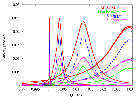
Figure 14.63: Comparisons among anomalous Drell-Yan in the MLSOM versus several anomaly-free models.

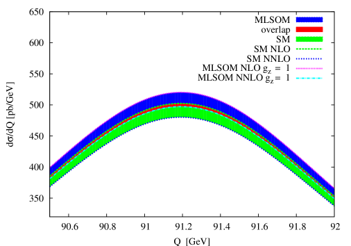
(a) Overlaps at NLO/NNLO

Figure 14.64: Zoom on the $Z$ resonance for anomalous Drell-Yan in the $\mu_{F}=\mu_{R}=Q$ at NLO/NNLO for all the models.

Bibliography

- [1] ALICE Collaboration, ALICE Physics Performance Report Volume I, J. Phys. G: Nucl. Part. Phys. 30 (2004) 1517-1763; CERN/LHCC 2003-049.
- [2] ALICE Collaboration, ALICE Physics Performance Report Volume II, J. Phys. G: Nucl. Part. Phys. 32 (2006) 1295-2040; CERN/LHCC 2005-030.
- [3] P. Giubellino et al, “Day-one proton–proton physics with the ALICE central detector”, ALICE Internal Note, ALICE-PHY-2000-28.
- [4] A. Dainese, “Measurement of heavy-flavour production with ALICE”, in these proceedings.
- [5] D. Stocco, “Quarkonia detection with the ALICE Muon Spectrometer in pp collisions at 14 TeV and PDF sensitivity in the low x region”, in these proceedings.
- [6] ALICE Collaboration, Addendum to the Technical Proposal: Electromagnetic Calorimeter, CERN/LHCC/2006-014.
- [7] ALICE Collaboration, Electromagnetic Calorimeter Technical Design Report, ALICE-TDR-014, CERN/LHCC/2008-014, 1 September 2008.
- [8] R. Caliandro, R. A. Fini and T. Virgili, 2002, ALICE Internal Note, ALICE-INT-2002-43.
- [9] T. Virgili, 2006, ALICE Internal Note, ALICE-INT-2006-013.
- [10] J. Conrad, J. G. Contreras and C. E. Jorgensen, 2005, ALICE Internal Note, ALICE-INT-2005-30.
- [11] R. Feynman, Phys. Rev. Lett. 23, 1415 (1969).
- [12] K. Alpgård et al. (UA5 Collaboration), Phys. Lett. B107, 310 (1981); G. J. Alner et al. (UA5 Collaboration), Z. Phys. C33, 1 (1986).
- [13] G. Arnison et al. (UA1 Collaboration), Phys. Lett. B123, 108 (1982).
- [14] F. Abe et al. (CDF Collaboration), Phys. Rev. D41, 2300 (1990).
- [15] A.B. Kaidalov, Phys. Lett. B116 (1982) 459; A.B. Kaidalov and K.A. Ter-Martirosyan, Phys. Lett. B117 (1982) 247; A. B. Kaidalov and O. I. Piskunova, Z. Phys. C 30 145 (1986); A. B. Kaidalov, Nucl. Phys. A 525, 39c (1991).
- [16] K.A. Ter-Martirosyan, Yad. Fiz. 44 (1986) 1257; Sov. J. Nucl. Phys. 44 (1986) 817.
- [17] A. B. Kaidalov, Physics-Uspekhi, 46 (11) 1121-1136 (2003).
- [18] R. Field (for the CDF Collaboration), “Min-bias and the underlying event in Run 2 at CDF”, Acta Phys. Polon. B 36 (2005) 167.
- [19] C.M.Buttar, D.Clements, I. Dawson and A.Moraes, “Simulations of minimum bias events and the underlying event, MC tuning and predictions for the LHC”, Acta Phys. Polon. B 35 (2004) 433; ATLAS Note ATLAS-PHYS-PUB-2005-007.
- [20] D.Acosta et al., “The underlying event at the LHC”, CMS Note 2006-067.
- [21] T. Sjostrand, P. Eden, C. Friberg, L.Lonnblad, G. Miu, S. Mrenna and E. Norrbin, Comput. Phys. Commun. 135 (2001) 238; arXiv:hep-ph/0010017.
- [22] J. M. Butterworth, J.R. Forshaw and M.H.Seymour, Z.Phys.C72 (1996) 637; arXiv:hep-ph/9601371.
- [23] T. Gleisberg, S. Hoche, F. Krauss, A. Schalicke. S. Schumann and J. C. Winter, JHEP 0402 (2004) 056; arXiv:hep-ph/0311263.
- [24] M. Bahr, S. Gieseke and M.H. Seymour, arXiv:hep-ph/0806.4250
- [25] R. Engel, Z.Phys.C66 (1995) 203.
- [26] J.F. Grosse-Oetringhaus and C. E. Jorgensen, 2007, ALICE Internal Note, ALICE-INT-2007-05.
- [27] W. Thome et al., Nucl. Phys. B 125, 365 (1977).
- [28] Z. Koba, H. B. Nielsen and P. Olesen, Nucl. Phys. B 40, 317 (1972).
- [29] G. J. Alner et al. (UA5 Collaboration), Phys. Lett. B138, 304 (1984).
- [30] A. Giovannini and R. Ugoccioni, Phys. Rev. D59 094020 (1999).
- [31] A. Giovannini and R. Ugoccioni, Phys. Rev. D60 074027 (1999).
- [32] J. Dias de Deus and R. Ugoccioni, Phys. Lett. B469 243 (1999).
- [33] W. D. Walker, Phys. Rev. D69 034007 (2004).
- [34] S. G. Matinyan and W. D. Walker, Phys. Rev. D59 034022 (1999).
- [35] T. Alexopoulos et al [E735 Collaboration], Phys. Lett. B435, 453 (1998).
- [36] V. Anykeev et al, Nucl. Instr. Meth. A303 350 (1991).
- [37] G.D’Agostini, DESY 94-099, June 1994.
- [38] R .E. Ansorge et al (UA5 Collaboration), Z. Phys. C43 357 (1989).
- [39] J.F. Grosse-Oetringhaus, 2008, ALICE Internal Note, ALICE-INT-2008-022.
- [40] L. Van Hove, Phys. Lett. B118 138 (1982).
- [41] B.Alper et al, Nucl. Phys. B 100 237 (1975); C. Albajar et al, Nucl. Phys. B 335 261 (1990); C. Abe et al, Phys. Rev. Lett. 61 1818 (1998).
- [42] P. Billoir, Nucl. Instr. Meth. A225 352 (1984).
- [43] G. Arnison et al (UA1 Collaboration) Phys. Lett B 118 173 (1982); G. Bocquet et al (UA1 Collaboration) Phys. Lett. B 366 434 (1996).
- [44] A. Breakstone et al Phys. Lett.B 132 458 (1983); A. Breakstone et al Phys. Lett.B 132 463 (1983); A. Breakstone et al Phys. Lett.B 183 227 (1987).
- [45] T. Alexopoulos T et al (E735 Collaboration) Phys. Rev. Lett. 64 991 (1990); T. Alexopoulos et al (E735 Collaboration) Phys. Rev. D 48 984 (1993).
- [46] D. Acosta et al (CDF Collaboration) Phys. Rev D 65 072005 (2002).
- [47] C. M.G. Lattes et al, Phys. Rep. 65 151 (1980).
- [48] X. N. Wang and R. C. Hwa, Phys.Rev. D 39 187 (1987); X. N. Wang and M. Gyulassy, Phys. Lett. B 282 466 (1992).
- [49] G. Corcella et al, JHEP 0101 (2001) 010; arXiv:hep-ph/0011363.
- [50] T. Affolder et al (CDF Collaboration], Phys. Rev. D 65 092002 (2002); D. Acosta et al (CDF Collaboration], Phys. Rev. D 70 072002 (2004).
- [51] A. Wroblewski, Acta. Phys. Polon. B16 (1985) 379.
- [52] V. V. Anisovich and M. N. Kobrinski, Phys. Lett. B52 (1974) 217; V. M. Shekhter and L. M. Scheglova, Sov. J. Nucl. Phys. 27 (1978) 567.
- [53] F. Becattini et al., Phys. Rev. C64 (2001) 024901.
- [54] F. Becattini, U. Heinz, Z. Phys. C76 (1997) 269; F. Becattini, M. Gazdzicki, J. Sollfrank, Eur. Phys. J. C5 (1998) 143; F. Becattini and G. Passaleva, Eur. Phys. J. C23 (2002) 551.
- [55] T. Alexopoulos et al. (E735 Collab.) Phys. Lett. B528 (2002) 43.
- [56] B.I. Abelev et al (STAR Collaboration) Phys. Rev. C75 (2007) 064901.
- [57] B. A. Kniehl, G. Kramer and B. Potter, Nucl. Phys. B597 (2001) 337.
- [58] D. DeFlorian, M. Stratmann and W. Vogelsang, Phys. Rev. D57 (1998) 5811.
- [59] S. Albino, B. A. Kniehl and G. Kramer, Phys. Lett. B725 (2005) 181.
- [60] G. Abbiendi et al. (OPAL Collab.), Eur. Phys.J. C16 (2000) 407.
- [61] Alexopoulos, T. et al. (E735 Collaboration), Phys. Rev. D48 (1993) 984.
- [62] L. Van Hove, Phys. Lett. B118 (1982) 138.
- [63] R. Vernet, “Prospects for strangeness measurements in ALICE”, Proceedings of the Workshop on Relativistic Nuclear Physics (WRNP07), June 2007, Kiev (Ukraine), Phys. Atom. Nucl. 71 (2008) 1523-1534; arXiv:nucl-ex/0802.0095v1.
- [64] A. Capella, U. Sukhatme, C.I. Tan and J. Tran Thanh Van, Phys. Rep. 236 (1994) 225.
- [65] B. Alper et al., Nucl. Phys. B100 (1975) 237; T. Akesson et al., Nucl. Phys. B228 (1983) 409; L. Camilleri et al., Phys. Rep. 53 (1987) 144.
- [66] G.C. Rossi, G. Veneziano, Nucl. Phys. B123 (1977) 507; Phys. Rep. 63 (1980) 149.
- [67] B.Z. Kopeliovich and B.G. Zakharov, Z. Phys. C43 (1989) 241.
- [68] D. Kharzeev, Phys. Lett. B378 (1996) 238.
- [69] B.Z. Kopeliovich and B. Povh, Z. Phys. C75 (1997) 693.
- [70] H1 Collaboration, C. Adloff et al., “Measurement of the baryon-antibaryon asymmetry in photoproduction at HERA”, Proceedings of 29th Int.Conference on High Energy Physics ICHEP98, Vancouver, Canada, July 1998.
- [71] B.Z. Kopeliovich and B. Povh, Phys. Lett. B446 (1999) 321.
- [72] I.G. Bearden et al. (BRAHMS Collaboration), Phys. Lett. B607 (2005) 42; arXiv:nucl-ex/0409002.
- [73] P. Christakoglou and M.Oldenburg, Private Communication, to be published as an ALICE Internal Note.
- [74] B. Buschbeck and H.C.Eggers, Nucl.Phys. (Proc.Suppl.) B92 (2001) 235; B. Buschbeck, H.C.Eggers and P.Lipa, Phys. Lett. B481 (2000) 187.
- [75] C. Lindsey (for the E735 Collaboration), FERMILAB-Conf-91/336
- [76] Z. Chajecki (for the STAR Collaboration), Proceedings of the conference Quark Matter 2005, Budapest, Hungary, August 4-9 2005, Nucl. Phys. A774 (2006) 599-602; arXiv:nucl-ex/0510014.
- [77] N.M.Agababyan et al (NA22 COLLAB.), Z.Phys.C59 (1993) 195.
- [78] T.Csörgö. M.Csanád, B.Lörstad and A.Ster, arXiv:hep-ph/0406042.
- [79] T. Humanic, Phys. Rev. C76 (2007) 025205.
- [80] I. Kawrakow, Phys. Rev. D49 (1994) 2275.
- [81] E. Berger, Nucl. Phys. B85 (1975) 61.
- [82] J. Ranft, Fortschr. Phys. 23 (1975) 467.
- [83] A. Giovannini and L. Van Hove, Z.Phys.C30 (1986) 391.
- [84] T.T. Chou and C.N.Yang, Phys. Lett. B135 (1984) 175.
- [85] S.L. Lim et al, Z.Phys.C43 (1989) 621; Z.Phys.C54 (1992) 107.
- [86] A. Giovannini and R. Ugoccioni, Phys. Lett. B558 (2003) 59.
- [87] X.N. Wang, Phys. Rev. D47 (1993) 2754.
- [88] J. Adams et al (STAR Collaboration) Nucl. Phys. A757 (2005) 102.
- [89] R.J. Porter and A.T. Trainor (for the STAR Collaboration), J.Phys.Conf.Ser. 27 (2005) 98; Acta Phys. Polonica B36 (2005) 353.
- [90] T.H. Burnett et al (JACEE COLLAB.), Phys. Rev. Lett. 50 (1983) 2062.
- [91] M. Adamus et al (NA22 COLLAB.), Phys. Lett. B185 (1987) 200.
- [92] R. Schicker, “Diffractive physics in ALICE”, Proceedings of 2th International Conference on Elastic and Diffractive Scattering “Forward Physics and QCD”, (DESY, Hamburg, 21 - 25 May 2007), DESY-PROC-2007-02; R. Schicker, “Low-mass diffractive systems at LHC”, Proc. of the conference “New Trends in high energy physics”, (Yalta, 15-22 Sep. 2007).
- [93] A. Bzdak, L. Motyka, L. Szymanowski,J. R. Cudell, Phys. Rev. D 75 (2007) 094023.
- [94] V. P. Goncalves, M. V. Machado, Phys. Rev. D 71 (2005) 014025.
- [95] V. P. Goncalves, M. V. Machado, Phys. Rev. D 75 (2007) 031502.
- [96] M. Gyulassy, I. Vitev, X. N. Wang and B. W. Zhang, Quark Gluon Plasma 3, edited by R. C. Hwa and X. N. Wang (World Scientific, Singapore, 2003), p.123; nucl-th/0302077.
- [97] R. Baier, Yu. L. Dokshitzer, A. J. Mueller and D. Schiff, Phys. Rev. C58, 1706 (1998).
- [98] R. Baier, D. Schiff and B. G. Zakharov, Ann. Rev. Nucl. Part. Sci.50, 37 (2000).
- [99] A. Kovner and U. A. Wiedemann in Ref.[96], p.192; hep-ph/0304151.
- [100] J. D. Bjorken, preprint FERMILAB-PUB-82-059-THY.
- [101] M. G. Mustafa, Phys. Rev. C 72, 014905 (2005).
- [102] A. K. Dutt-Mazumder, J. Alam, P. Roy and B. Sinha, Phys. Rev. D 71, 094016 (2005).
- [103] M. Djordjevic, Phys. Rev. C 74, 064907 (2006).
- [104] M. Djordjevic, M. Gyulassy, R. Vogt and S. Wicks, Phys. Lett. B 632, 81 (2006).
- [105] A. Morsch, J. Phys. G31 (2005) S597.
- [106] M. Heinz (for the STAR Collaboration), “Systematic studies of fragmentation functions in inclusive jets from p+p collisions at 200 GeV by STAR”, Hard Probes Conference 2008 (HP08), Illa de Toxa, Galicia, Spain, 8-14 June 2008.
- [107] N. Armesto, “Jet rates in p+A collisions at the LHC”, Workshop on Proton-Nucleus Collisions at the LHC (CERN, 25-27 May 2005), A. Accardi et al., PDFs, shadowing and pA collisions, “Hard Probes in heavy-ion collisions at the LHC”, CERN Yellow Report 2004-009, hep-ph/0308248.
- [108] C. A. Loizides. Ph. D. Thesis, Univ. of Frankfurt am Main, Germany, arXiv:nucl-ex/0501017.
- [109] R. M. Tornbull, J. Phys. G14, 135 (1988).
- [110] P. Aurenche, M. Fontannaz, J.-Ph. Guillet, B. Kniehl, E. Pilon and M. Werlen, Eur. Phys. J. C9, 107 (1999).
- [111] P. Aurenche, M. Fontannaz, J.-Ph. Guillet, B. Kniehl, E. Pilon and M. Werlen, Eur. Phys. J. C13, 347 (2000); hep-ph/9910252.
- [112] T. Binoth et al., Eur. Phys. J. C16, 311 (2000).
- [113] S. Catani et al., J. High Energy Phys. 05, 028 (2002).
- [114] V. M. Abazov et al., (D0 Collaboration), Phys. Lett. B639, 151 (2006).
- [115] S. S. Adler et al. (PHENIX Collaboration), Phys. Rev. D71, 071102 (2005).
- [116] P. Aurenche, M. Fontannaz, J.-Ph. Guillet, E. Pilon and M. Werlen, Phys. Rev. D73, 094007 (2006).
- [117] L. Apanasievich et al., (E706 Collaboration), Phys. Rev.D70, 092009 (2004).
- [118] E. Laenen, G. Sterman and W. Vogelsang, Phys. Rev. Lett. 84, 4296 (2000); Phys. Rev. D63 114018 (2001).
- [119] H.-L. Lai and H.-N. Li, Phys. Rev. D58, 114020 (1998).
- [120] L.E. Gordon and W. Vogelsang, Phys. Rev. D 48 3136 (1993).
- [121] F. Arleo et al., J. High Energy Phys. 11, 009 (2004).
- [122] F. Arleo et al., Photon Physics in heavy-ion collisions at the LHC, CERN Yellow Report 2004-009; hep-ph/0311131.
- [123] J. Ranft, Phys. Rev. D51, 64 (1995); R. Engel, Z. Phys. C66, 203 (1995); R. Engel and J. Ranft, Phys. Rev. D54, 4244 (1996); S. Roesler, R. Engel and J. Ranft, hep-ph/0012252.
- [124] L. Bourhis, M. Fontannaz and J.-Ph. Guillet, Eur. Phys. J. C2, 529 (1998) 529.
- [125] G. Conesa et al., Nucl. Inst. Meth.A 537 363 (2005).
- [126] G. Conesa et al., ALICE-INT-2005-014, (2005).
- [127] B.A. Kniehl, G. Kramer and B. Potter, Nucl. Phys. B582, 514 (2000).
- [128] J. Jalilian-Marian, K. Orginos and I. Sarcevic, Phys. Rev. C 63 041901 (2001); hep-ph/0010230.
- [129] C. Wong and H. Wang, Phys. Rev. C 58 376 (1998).
- [130] G. Papp, P. Lévai, and G. Fai, Phys. Rev. C 61, 0219021 (1999).
- [131] B.G. Zakharov, JETP Lett. 80, 1 (2004).
- [132] C. A. Salgado and U. A. Wiedemann, Phys. Rev. Lett. 93 042301 (2004).
- [133] T. Humanic, ALICE Internal Report, ALICE-INT-2005-017;
- [134] T. J. Humanic, B. Koch and H. Stocker, arXiv:hep-ph/0607097.
- [135] C. M. Harris, P. Richardson and B. R. Webber, arXiv:hep-ph/0409309.

Bibliography

- [1] ALICE Collaboration, Physics Performance Report Vol. I, CERN/LHCC 2003-049 and J. Phys. G 30, 1517 (2003).
- [2] N. Carrer and A. Dainese, ALICE Internal Note, ALICE-INT-2003-019 (2003), arXiv:hep-ph/0311225.
- [3] M.L. Mangano, P. Nason and G. Ridolfi, Nucl. Phys. B 373, 295 (1992).
- [4] K.J. Eskola, V.J. Kolhinen, C.A. Salgado, Eur. Phys. J. C 9, 61 (1999).
- [5] M. Monteno, these proceedings.
- [6] D. Stocco, these proceedings.
- [7] ALICE Collaboration, Physics Performance Report Vol. II, CERN/LHCC 2005-030 and J. Phys. G 32 1295, (2006).
- [8] M. Cacciari, S. Frixione, M.L. Mangano, P. Nason and G. Ridolfi, JHEP 0407, 033 (2004).
- [9] M. Cacciari, private communication.
- [10] C. Albajar et al., UA1 Collaboration, Phys. Lett. B 213, 405 (1988); Phys. Lett. B 256, 121 (1991).
- [11] A. Dainese, arXiv:nucl-ex/0608005.
- [12] J. Baines et al., arXiv:hep-ph/0601164, in CERN-2005-014 / DESY-PROC-2005-01.

Bibliography

- [1] ALICE Collaboration, LHCC 99-22 / ALICE TDR 5.
- [2] V. D. Barger and W. Y. Keung and R. J. Phillips, Phys. Lett. B91 (1980) 253.
- [3] M. Bedjidian et al., CERN YellowReport, CERN-2004-009, [arXiv:hep-ph/0311048].
- [4] A. D. Martin, R. G. Roberts, W. J. Stirling and R. S. Thorne, Eur. Phys. J. C 4 (1998) 463 [arXiv:hep-ph/9803445].
- [5] D. Acosta et al. [CDF Collaboration], Phys. Rev. D 71 (2005) 032001 [arXiv:hep-ex/0412071].
- [6] D. Acosta et al. [CDF Collaboration], Phys. Rev. Lett. 88, 161802 (2002).
- [7] N. Carrer and A. Dainese, ALICE Internal Note 2003–019, [arXiv:hep-ph/0311225].
- [8] ALICE Collaboration, ALICE Physics Performance Report Volume II, J. Phys. G: Nucl. Part. Phys. 32 1295-2040.
- [9] ALICE Collaboration, ALICE Physics Performance Report Volume I, J. Phys. G: Nucl. Part. Phys. 30 1517-1763.
- [10] A. D. Martin, R. G. Roberts, W. J. Stirling and R. S. Thorne, Phys. Lett. B 531 (2002) 216 [arXiv:hep-ph/0201127].
- [11] H. L. Lai et al. [CTEQ Collaboration], Eur. Phys. J. C 12, 375 (2000) [arXiv:hep-ph/9903282].
- [12] J. Pumplin, D. R. Stump, J. Huston, H. L. Lai, P. Nadolsky and W. K. Tung, JHEP 0207 (2002) 012 [arXiv:hep-ph/0201195].

Bibliography

- [1] J.M. Campbell, J.W. Huston, W.J. Stirling, Hard Interactions of Quarks and Gluons: A Primer for LHC Physics. Rept. Prog. Phys. 70:89 (2007).
- [2] R. Devenish, A. Cooper-Sarkar Deep Inelastic Scattering. Oxford University Press, Oxford (2004).
- [3] S. Ferrag, Proton structure impact on sensitivity to extra-dimensions at LHC. hep-ph/0407303 (2004).
- [4] A. Djouadi, S. Ferrag, PDF uncertainties in Higgs production at hadron colliders. Phys. Lett. B 586 345-352 (2004).
- [5] D.Phil. thesis by F. Heinemann (Oxford) 2007.
- [6] A. Tricoli for the ATLAS Coll. Structure function measurements at the LHC. Acta Phys. Polon. B 37 711-714 (2006).
- [7] Ph.D. thesis by I. Hollins (Birmingham) 2006.
- [8] S. Diglio, A. Tonazzo and M. Verducci (RomaTre) 2005.
- [9] ATLAS CSC Note Electroweak boson cross-section measurements with ATLAS (2008).
- [10] C. Anastasiou, L. Dixon, K. Melnikov, F. Petriello, High precision QCD at hadron colliders: Electroweak gauge boson rapidity distributions at NNLO. Phys. Rev. D 69 094008 (2004).
- [11] Thanks to C. Carloni and G. Polesello.
- [12] A. Cooper-Sarkar (Oxford) and A. Tricoli (RAL) 2006.
- [13] D.Phil. thesis by A. Tricoli (Oxford) 2006.
- [14] A. Tricoli, A. Cooper-Sarkar, C. Gwenlan, Uncertainties on W and Z production at the LHC. CERN-2005-014, FERMILAB-CONF-05-586-E, IFUM-853-FT, hep-ex/0509002 (2005).
- [15] A. Cooper-Sarkar (Oxford) private communication, 2005.
- [16] T. Carli, G. P. Salam, F. Siegert, A posteriori inclusion of PDFs in NLO QCD final-state calculations. hep-ph/0510324 (2005).
- [17] T. Carli, D. Clements, Cooper-Sarkar, C. Gwenlan, A. G. P. Salam, P. Starovoitov, M Sutton, “PDF4LHC” meeting (2008).

Bibliography

- [1] R. Hamberg, W.L. van Neerven, T. Matsuura, Nucl.Phys. B 359 343, (1991), Erratum-ibid.B 644 403, (2002). W. Van Neerven and A. Vogt, Nucl.Phys. B 603, 42, (2001); Nucl.Phys. B 588, 345, (2000).
- [2] S. Catani, D. de Florian, M. Grazzini, P. Nason, JHEP 0307 028, (2003); G. Corcella and L. Magnea, Phys.Rev.72,074017, (2005); V. Ravindran, J. Smith, W.L. van Neerven,hep-ph/0608308.
- [3] C. Anastasiou, L. J. Dixon, K. Melnikov and F. Petriello Phys.Rev. D 69, 094008, (2004).
- [4] K. Melnikov and F. Petriello, Phys.Rev.D74114017, (2006).
- [5] S. Moch, J. Vermaseren and A. Vogt, Nucl. Phys. B 688, 101, (2004); Nucl. Phys. B 691, 129, (2004).
- [6] The QCD / SM working group: Summary report. W. Giele et al, hep-ph/0204316, (2002)
- [7] Working Group I: Parton distributions: Summary report for the HERA LHC Workshop Proceedings. M. Dittmar et. al., hep-ph/0511119, (2005)
- [8] A. Cafarella,C. Corianò and M. Guzzi Comput.Phys.Commun. 179, 665 (2008), arXiv:0803.0462 [hep-ph]
- [9] A. Cafarella, C. Corianò, M. Guzzi, JHEP 0708, 030 (2007), hep-ph/0702244.
- [10] A. Cafarella, C. Corianò, M. Guzzi Nucl.Phys. B 748, 253 (2006), hep-ph/0512358; A. Cafarella and C. Corianò, Comput.Phys.Commun. 160, 213 (2004), hep-ph/0311313.
- [11] A. Vogt, Comput.Phys.Commun. 170 65, (2005).
- [12] S.I. Alekhin, Phys.Rev.D 68, 014002, (2003); S.I. Alekhin, Eur.Phys.J. C 10, 395, (1999);
- [13] A.D. Martin, R.G. Roberts, W.J. Stirling and R.S. Thorne, Eur.Phys.J. C 23, 73 (2002); Phys.Lett.B 531, 216 (2002).
- [14] C. Corianò, A. E. Faraggi and M. Guzzi, Eur.Phys.J.C53, 421 (2008), arXiv:0704.1256 [hep-ph].
- [15] R. Armillis, C. Corianò and M. Guzzi, JHEP 0805, 015 (2008), arXiv:0711.3424 [hep-ph]
- [16] C. Corianò, M. Guzzi and S. Morelli, Eur.Phys.J.C 55, 629 (2008), arXiv:0801.2949 [hep-ph]
- [17] C. Corianò, A.E. Faraggi and M. Guzzi, Phys.Rev.D 78, 015012 (2008), arXiv:0802.1792 [hep-ph]
- [18] R. Armillis, C. Corianò, M. Guzzi and S. Morelli, JHEP 0810, 034 (2008), arXiv:0808.1882 [hep-ph]
- [19] R. Armillis, C. Corianò, M. Guzzi and S. Morelli, arXiv:0809.3772 [hep-ph]

Bibliography

- [1] U. Baur, Electroweak physics at the Tevatron and LHC: Theoretical status and perspectives, arXiv:hep-ph/0511064
- [2] R. Armilis, C. Corianò, A. E. Faraggi, M. Guzzi, N. Irges, Extra neutral interactions at the LHC, these proceedings
- [3] Q.-H. Cao and C.-P. Yuan, Phys. Rev. Lett. 93 (2004) 042001; arXiv:hep-ph/0401171
- [4] B.F.L. Ward and S.A. Yost, Acta Phys. Polon. B38 (2007) 2395
- [5] S. Jadach, W. Placzek, M. Skrzypek, P. Stephens and Z. Was, Acta Phys. Polon. B38 (2007) 2305
-
[6]
A. Tricoli, Parton densities at the LHC, these proceedings;
A. Cafarella, C. Corianò and M. Guzzi, NNLO evolution of Pdf’s, these proceedings;
N.E. Adam, V. Halyo and S.A. Yost, arXiv:0802.3251 [hep-ph];
S. Frixione and M.L. Mangano, JHEP 0405 (2004) 056 - [7] G. Altarelli, R. K. Ellis and G. Martinelli, Nucl. Phys. B157 (1979) 461
- [8] R. Hamberg, W. L. van Neerven and T. Matsuura, Nucl. Phys. B359 (1991) 343 [Erratum Nucl. Phys. B644 (2002) 403]
- [9] W.T. Giele, E.W.N. Glover and D.A. Kosower, Nucl. Phys. B403 (1993) 633
- [10] J.M. Campbell and R.K. Ellis, Phys. Rev. D65 (2002) 113007
- [11] C. Balazs and C. P. Yuan, Phys. Rev. D56 (1997) 5558
- [12] F. Landry, R. Brock, P.M. Nadolsky and C.-P. Yuan, Phys. Rev. D67 (2003) 073016
- [13] S. Frixione and B. R. Webber, JHEP 0206 (2002) 029
- [14] S. Frixione, P. Nason and C. Oleari, JHEP 0711 (2007) 070
- [15] K. Melnikov and F. Petriello, Phys. Rev. Lett. 96 (2006) 231803
- [16] K. Melnikov and F. Petriello, Phys. Rev. D74 (2006) 114017
- [17] M.L. Mangano, M. Moretti, F. Piccinini, R. Pittau and A.D. Polosa, JHEP 0307 (2003) 001
- [18] T. Stelzer and W.F. Long, Comp. Phys. Commun. 81 (1994) 357; F. Maltoni and T. Stelzer, JHEP 02 (2003) 027
- [19] A. Kanaki and C.G. Papadopoulos, Comput. Phys. Commun. 132 (2000) 306; C.G. Papadopoulos and M. Worek, Eur. Phys. J. C50 (2007) 843; A. Cafarella, C.G. Papadopoulos and M. Worek, arXiv:0710.2427 [hep-ph].
- [20] T. Gleisberg, S. Höche, F. Krauss, A. Schälicke, S. Schumann and J. Winter, JHEP 0402 (2004) 056
- [21] S. Dittmaier and M. Krämer, Phys. Rev. D65 (2002) 0703007
- [22] U. Baur and D. Wackeroth, Phys. Rev. D70 (2004) 073015
- [23] V. A. Zykunov, Eur. Phys. J. Direct C3 (2001) 9; Phys. Atom. Nucl. 69 (2006) 1522
- [24] A. Arbuzov, D. Bardin, S. Bondarenko, P. Christova, L. Kalinovskaya, G. Nanava and R. Sadykov, Eur. Phys. J. C46 (2006) 407
- [25] C.M. Carloni Calame, G. Montagna, O. Nicrosini and A. Vicini, JHEP 12 (2006) 016
- [26] U. Baur, O. Brein, W. Hollik, C. Schappacher and D. Wackeroth, Phys. Rev. D65 (2002) 033007
- [27] V.A. Zykunov, Phys. Rev. D75 (2007) 073019
- [28] C.M. Carloni Calame, G. Montagna, O. Nicrosini and A. Vicini, JHEP 10 (2007) 109
- [29] A. Arbuzov, D. Bardin, S. Bondarenko, P. Christova, L. Kalinovskaya, G. Nanava and R. Sadykov, arXiv:0711.0625 [hep-ph]
- [30] C. Buttar et al., arXiv:hep-ph/0604120
- [31] C.E. Gerber et al., FERMILAB-CONF-07-052, arXiv:0705.3251 [hep-ph]
- [32] C. Buttar et al., arXiv:0803.0678 [hep-ph]
- [33] C.M. Carloni Calame, G. Montagna, O. Nicrosini and M. Treccani, Phys. Rev. D69 (2004) 037301
- [34] C.M. Carloni Calame G. Montagna, O. Nicrosini and M. Treccani, JHEP 05 (2005) 019
- [35] S. Jadach and W. Płaczek, Eur. Phys. J. C29 (2003) 325
- [36] S. Brensing, S. Dittmaier, M. Krämer and A. Muck, arXiv:0710.3309 [hep-ph]
- [37] U. Baur, Phys. Rev. D75 (2007) 013005
- [38] W. Hollik, T. Kasprzik and B.A. Kniehl, Nucl. Phys. B790 (2008) 138
- [39] J.H. Kühn, A. Kulesza and S. Pozzorini, Nucl. Phys. B797 (2008) 27
- [40] E. Maina, S. Moretti and D.A. Ross, Phys. Lett. 593 (2004) 143, Erratum ibid. 614 (2005) 216.
- [41] A.D. Martin, R.G. Roberts, W.J. Stirling and R.S. Thorne, Eur. Phys. J. C39 (2005) 155
- [42] U. Baur et al., The neutral-current Drell-Yan process in the high invariant mass region, in [32]

Bibliography

- [1] S. G. Gorishnii, A. L. Kataev and S. A. Larin, Phys. Lett. B 259 (1991) 144; L. R. Surguladze and M. A. Samuel, Phys. Rev. Lett. 66 (1991) 560 [Erratum-ibid. 66 (1991) 2416]; K. G. Chetyrkin, Phys. Lett. B 391 (1997) 402.
- [2] R. Hamberg, W. L. van Neerven and T. Matsuura, Nucl. Phys. B 359 (1991) 343 [Erratum-ibid. B 644 (2002) 403]; E. B. Zijlstra and W. L. van Neerven, Nucl. Phys. B 383 (1992) 525; E. B. Zijlstra and W. L. van Neerven, Phys. Lett. B 297 (1992) 377.
- [3] R. V. Harlander and W. B. Kilgore, Phys. Rev. Lett. 88 (2002) 201801; C. Anastasiou and K. Melnikov, Nucl. Phys. B 646 (2002) 220; V. Ravindran, J. Smith and W. L. van Neerven, Nucl. Phys. B 665 (2003) 325.
- [4] C. Anastasiou, K. Melnikov and F. Petriello, Phys. Rev. D 69 (2004) 076010.
- [5] T. Binoth and G. Heinrich, Nucl. Phys. B 585 (2000) 741, Nucl. Phys. B 693 (2004) 134; K. Hepp, Commun. Math. Phys. 2 (1966) 301.
- [6] C. Anastasiou, K. Melnikov and F. Petriello, Phys. Rev. Lett. 93 (2004) 032002.
- [7] C. Anastasiou, K. Melnikov and F. Petriello, Phys. Rev. Lett. 93 (2004) 262002, Nucl. Phys. B 724 (2005) 197.
- [8] K. Melnikov and F. Petriello, Phys. Rev. Lett. 96 (2006) 231803, Phys. Rev. D 74 (2006) 114017.
- [9] C. Anastasiou, K. Melnikov and F. Petriello, arXiv:hep-ph/0505069.
- [10] R. K. Ellis, D. A. Ross and A. E. Terrano, Nucl. Phys. B 178 (1981) 421.
- [11] K. Fabricius, I. Schmitt, G. Kramer and G. Schierholz, Z. Phys. C 11 (1981) 315.
- [12] W. T. Giele and E. W. N. Glover, Phys. Rev. D 46 (1992) 1980; W. T. Giele, E. W. N. Glover and D. A. Kosower, Nucl. Phys. B 403 (1993) 633.
- [13] S. Frixione, Z. Kunszt and A. Signer, Nucl. Phys. B 467 (1996) 399; S. Frixione, Nucl. Phys. B 507 (1997) 295.
- [14] S. Catani and M. H. Seymour, Nucl. Phys. B 485 (1997) 291 [Erratum-ibid. B 510 (1997) 503].
- [15] D. A. Kosower, Phys. Rev. D 57 (1998) 5410, Phys. Rev. D 67 (2003) 116003, Phys. Rev. D 71 (2005) 045016.
- [16] S. Weinzierl, JHEP 0303 (2003) 062, JHEP 0307 (2003) 052.
- [17] S. Frixione and M. Grazzini, JHEP 0506 (2005) 010.
- [18] A. Gehrmann-De Ridder, T. Gehrmann and E. W. N. Glover, Phys. Lett. B 612 (2005) 36, Phys. Lett. B 612 (2005) 49, JHEP 0509 (2005) 056; A. Daleo, T. Gehrmann and D. Maitre, hep-ph/0612257.
- [19] G. Somogyi, Z. Trocsanyi and V. Del Duca, JHEP 0506 (2005) 024, JHEP 0701 (2007) 070; G. Somogyi and Z. Trocsanyi, JHEP 0701 (2007) 052.
- [20] A. Gehrmann-De Ridder, T. Gehrmann and E. W. N. Glover, Nucl. Phys. B 691 (2004) 195.
- [21] S. Weinzierl, Phys. Rev. D 74 (2006) 014020.
- [22] A. Gehrmann-De Ridder, T. Gehrmann, E. W. N. Glover and G. Heinrich, Nucl. Phys. Proc. Suppl. 160 (2006) 190.
- [23] A. Gehrmann-De Ridder, T. Gehrmann, E. W. N. Glover and G. Heinrich, JHEP 0712 (2007) 094 [arXiv:0711.4711 [hep-ph]].
- [24] S. Catani and M. Grazzini, Phys. Rev. Lett. 98 (2007) 222002 [arXiv:hep-ph/0703012].
- [25] M. Grazzini, JHEP 0802 (2008) 043 [arXiv:0801.3232 [hep-ph]].
- [26] S. Catani, D. de Florian and M. Grazzini, JHEP 0201 (2002) 015.
- [27] G. Parisi and R. Petronzio, Nucl. Phys. B 154 (1979) 427.
- [28] J. C. Collins, D. E. Soper and G. Sterman, Nucl. Phys. B 250 (1985) 199.
- [29] S. Catani, D. de Florian and M. Grazzini, Nucl. Phys. B 596 (2001) 299.
- [30] G. Bozzi, S. Catani, D. de Florian and M. Grazzini, Phys. Lett. B 564 (2003) 65, Nucl. Phys. B 737 (2006) 73, Nucl. Phys. B 791 (2008) 1.
- [31] M. Grazzini, JHEP 0601 (2006) 095.
- [32] D. de Florian and M. Grazzini, Phys. Rev. Lett. 85 (2000) 4678, Nucl. Phys. B 616 (2001) 247.
- [33] S. Catani, M. Grazzini, to appear.
- [34] D. de Florian, M. Grazzini and Z. Kunszt, Phys. Rev. Lett. 82 (1999) 5209; see also J. Campbell and R.K. Ellis, MCFM - Monte Carlo for FeMtobarn processes, http://mcfm.fnal.gov.
- [35] A. D. Martin, R. G. Roberts, W. J. Stirling and R. S. Thorne, Phys. Lett. B 604 (2004) 61.
- [36] CMS collaboration, CMS Physics, Technical Design Report, Vol. II Physics Performance, report CERN/LHCC 2006-021.
- [37] S. Catani and B. R. Webber, JHEP 9710 (1997) 005.
- [38] G. Davatz, G. Dissertori, M. Dittmar, M. Grazzini and F. Pauss, JHEP 0405 (2004) 009.
- [39] S. Catani, Y. L. Dokshitzer, M. H. Seymour and B. R. Webber, Nucl. Phys. B 406 (1993) 187; S. D. Ellis and D. E. Soper, Phys. Rev. D 48 (1993) 3160.
- [40] C. Anastasiou, G. Dissertori and F. Stockli, JHEP 0709 (2007) 018.
- [41] http://theory.fi.infn.it/grazzini/codes.html

Bibliography

- [1] J. C. Collins, D. E. Soper and G. Sterman, Adv. Ser. Direct. High Energy Phys. 5 (1988) 1.
- [2] Y. L. Dokshitzer, D. Diakonov and S. I. Troyan, Phys. Rept. 58 (1980) 269; J. G. M. Gatheral, Phys. Lett. B 133 (1983) 90; A. Bassetto, M. Ciafaloni and G. Marchesini, Phys. Rept. 100 (1983) 201.
- [3] S. Catani, D. de Florian, M. Grazzini and P. Nason, JHEP 0307 (2003) 028; G. Bozzi, S. Catani, D. de Florian and M. Grazzini, Nucl. Phys. B 737(2006)73.
- [4] G. Corcella et al., JHEP 0101 (2001) 010.
- [5] T. Sjostrand, S. Mrenna and P. Skands, JHEP 0605 (2006) 026.
- [6] T. Sjostrand and P. Z. Skands, Eur. Phys. J. C 39 (2005) 129.
- [7] L. Lonnblad, Comput. Phys. Commun. 71 (1992) 15.
- [8] M. Dasgupta and G. P. Salam, J. Phys. G 30 (2004) R143.
- [9] A. Banfi, G. P. Salam and G. Zanderighi, JHEP 0503 (2005) 073.
-
[10]
M. Dasgupta and G. P. Salam,
Phys. Lett. B 512 (2001) 323;
JHEP 0203 (2002) 017. - [11] A. Banfi, G. Corcella and M. Dasgupta, JHEP 0703 (2007) 050.
- [12] R. B. Appleby and M. H. Seymour, JHEP 0212 (2002) 063.
- [13] A. Banfi and M. Dasgupta, Phys. Lett. B 628 (2005) 49.
- [14] J. R. Forshaw, A. Kyrieleis and M. H. Seymour, JHEP 0608 (2006) 059.
- [15] A. Banfi, G. P. Salam and G. Zanderighi, JHEP 0408 (2004) 062.
- [16] Z. Nagy, Phys. Rev. D 68 (2003) 094002.

Bibliography

- [1] SLD Collaboration, K. Abe et al., Phys. Rev. Lett. 84 (2000) 4300.
- [2] ALEPH Collaboration, A. Heister et al., Phys. Lett. B512 (2001) 30.
- [3] OPAL Collaboration, G. Abbiendi et al., Eur. Phys. J. C29 (2003) 463.
- [4] DELPHI Collaboration, G. Barker et al., DELPHI 2002-069, CONF 603.
- [5] D. Shirkov, Nucl. Phys. Proc. Suppl. 152 (2006) 51.
- [6] U. Aglietti, G. Corcella and G. Ferrera, Nucl. Phys. B775 (2007) 162.
- [7] G. Corcella and G. Ferrera, JHEP 0712 (2007) 029.
- [8] B. Mele and P. Nason, Nucl. Phys. B 361 (1991) 626.
- [9] G. Altarelli and G. Parisi, Nucl. Phys. B126 (1977) 298.
-
[10]
V.N. Gribov and L.N. Lipatov, Sov. J. Nucl. Phys. 15 (1972) 438;
L.N. Lipatov, Sov. J. Nucl. Phys. 20 (1975) 95;
Yu.L. Dokshitzer, Sov. Phys. 46 (1977) 641. - [11] M. Cacciari and S. Catani, Nucl. Phys. B617 (2001) 253.
- [12] G. Corcella, I.G. Knowles, G. Marchesini, S. Moretti, K. Odagiri, P. Richardson, M.H. Seymour, B.R. Webber, JHEP 0101 (2001) 010.
- [13] T. Sjostrand, S. Mrenna and P. Skands, JHEP 0605 (2006) 026.
- [14] G. Marchesini and B.R. Webber, Nucl. Phys. B238 (1984) 1; ibid. B310 (1988) 461.
- [15] V.G. Kartvelishvili, A.K. Likehoded and V.A. Petrov, Phys. Lett. B78 (1978) 615.
- [16] B.R. Webber, Nucl. Phys. B238 (1984) 492.
- [17] B. Andersson, G. Gustafson, G. Ingelman, T. Sjöstrand, Phys. Rept. 97 (1983) 31.
- [18] T. Sjöstrand and P.Z. Skands, Eur. Phys. J. C39 (2005) 129.
- [19] A. Banfi, G. Corcella and M. Dasgupta, JHEP 0703 (2007) 050.
- [20] S. Catani, G. Marchesini and B.R. Webber, Nucl. Phys. B349 (1991) 635.
- [21] G. Corcella and V. Drollinger, Nucl. Phys. B730 (2005) 82.
- [22] M.G. Bowler, Z. Phys. C11 (1981) 169.
- [23] G. Corcella and A.D. Mitov, Nucl. Phys. B623 (2002) 247.
- [24] M. Cacciari, G. Corcella and A.D. Mitov, JHEP 0212 (2002) 015.
- [25] G. Corcella, Nucl. Phys. B 705 (2005) 363 [Erratum-ibid. B 715 (2005) 609].
- [26] M. Cacciari and P. Nason, Phys. Rev. Lett. 89 (2002) 122003.

Bibliography

- [1] S. Hoche, F. Krauss, N. Lavesson, L. Lonnblad, M. Mangano, A. Schalicke and S. Schumann, arXiv:hep-ph/0602031.
- [2] S. Frixione and B. R. Webber, arXiv:hep-ph/0601192.
- [3] S. Frixione and B. R. Webber, JHEP 0206 (2002) 029 [arXiv:hep-ph/0204244].
- [4] S. Frixione, P. Nason and B. R. Webber, JHEP 0308 (2003) 007 [arXiv:hep-ph/0305252].
- [5] M.L. Mangano, presentation at the FNAL Matrix Element/Monte Carlo Tuning Working Group, 15 Nov 2002, http://www-cpd.fnal.gov/personal/mrenna/tuning/nov2002/mlm.pdf .
- [6] M. L. Mangano, M. Moretti, F. Piccinini and M. Treccani, JHEP 0701, 013 (2007) [arXiv:hep-ph/0611129].
-
[7]
M. L. Mangano, M. Moretti, F. Piccinini, R. Pittau and A. D. Polosa,
JHEP 0307 (2003) 001
[arXiv:hep-ph/0206293];
F. Caravaglios, M. L. Mangano, M. Moretti and R. Pittau, Nucl. Phys. B 539 (1999) 215 [hep-ph/9807570]. - [8] G. Marchesini and B. R. Webber, Nucl. Phys. B 310 (1988) 461. G. Marchesini, B. R. Webber, G. Abbiendi, I. G. Knowles, M. H. Seymour and L. Stanco, Comput. Phys. Commun. 67 (1992) 465. G. Corcella et al., JHEP 0101 (2001) 010 [hep-ph/0011363]. G. Corcella et al., “HERWIG 6.5 release note,” arXiv:hep-ph/0210213.
- [9] A. D. Martin, R. G. Roberts, W. J. Stirling and R. S. Thorne, Eur. Phys. J. C 23 (2002) 73 [arXiv:hep-ph/0110215].
- [10] F.E. Paige and S.D. Protopopescu, in Physics of the SSC, Snowmass, 1986, Colorado, edited by R. Donaldson and J. Marx.
- [11] P. Nason, JHEP 0411 (2004) 040 [arXiv:hep-ph/0409146].
- [12] P. Nason and G. Ridolfi, JHEP 0608 (2006) 077 [arXiv:hep-ph/0606275].
- [13] P. Nason, presented in this Meeting
———————————————————————-

Bibliography

- [1] G. Corcella, I.G. Knowles, G. Marchesini, S. Moretti, K. Odagiri, P. Richardson, M.H. Seymour, B.R. Webber, JHEP 0101 (2001) 010.
- [2] T. Sjostrand, S. Mrenna and P. Skands, JHEP 0605 (2006) 026.
- [3] G. Bozzi, S. Catani, D. de Florian and M. Grazzini, Phys. Lett. B564 (2003) 65; Nucl. Phys. B 737 (2006) 73.
- [4] G. Marchesini and B.R. Webber, Nucl. Phys. B238 (1984) 1; Nucl. Phys. B310 (1988) 461.
- [5] H.U. Bengtsson and G. Ingelman, Comput. Phys. Commun. 34 (1985) 251.
- [6] M.H. Seymour, Comput. Phys. Commun. 90 (1995) 95.
- [7] G. Miu and T. Sjostrand, Phys. Lett. B449 (1999) 313.
- [8] B.R. Webber, Nucl. Phys. B238 (1984) 492.
- [9] B. Andersson, G. Gustafson, G. Ingelman, T. Sjöstrand, Phys. Rept. 97 (1983) 31
- [10] G. Corcella, Bottom-quark fragmentation: resummations and Monte Carlo simulations, these proceedings.
- [11] J. Pumplin, D.R. Stump, J. Huston, H.L. Lai and P. Nadolsky, JHEP 0207 (2002) 012.
- [12] W.M. Yao et al., J. Phys. G33, (2006) 1.
-
[13]
C. Anastasiou and K. Melnikov, Nucl. Phys. B646 (2002) 220;
V. Ravindran, J. Smith and W.L. van Neerven, Nucl. Phys. B634 (2002) 247. - [14] S. Catani, G. Marchesini and B.R. Webber, Nucl. Phys. B349 (1991) 635.
- [15] A. Djouadi, J. Kalinowski and M. Spira, Comput. Phys. Commun. 108 (1998) 56.
- [16] M.H. Seymour, private communication.
- [17] G. Corcella and D. Rebuzzi, work in progress.
- [18] U. Baur and E.W.N. Glover, Nucl. Phys. B339 (1990) 38.
- [19] M. Spira, A. Djouadi, D. Graudenz and P.M. Zerwas, Nucl. Phys. B453 (1995) 17..
- [20] G. Corcella and S. Moretti, Phys. Lett. B590 (2004) 249.
- [21] G. Corcella and M.H. Seymour, Nucl. Phys. B565 (2000) 227.
- [22] S. Frixione and B.R. Webber, JHEP 0206 (2002) 029.

Bibliography

- [1] E.Boos, A.Djouadi, M.Muhlleitner, and A.Vologdin, “The MSSM Higgs bosons in the intense-coupling regime,” Phys.Rev. D66(2002) 055004, arXiv:hep-ph/0205160.
- [2] E.Boos, A.Djouadi, and A.Nikitenko, “Detection of the MSSM Higgs bosons in the intense-coupling regime at the LHC,” Phys.Lett. B578(2004) 384-393, arXiv:hep-ph/0307079.
- [3] ALEPH, DELPHI, L3, OPAL Collaboration, LEP Working Group for Higgs Boson Searches, “Search for neutral MSSM Higgs bosons at LEP,” arXiv:hep-ex/0602042.
- [4] LEP Working Group for Higgs Boson Searches, “Search for Charged Higgs bosons: Preliminary combined results using LEP data collected at energies up to 209 GeV,” arXiv:hep-ex/0107031.
- [5] D.Acosta et al. [CMS Collaboration], “CMS Coll. Physics TDR Vol.II, Chapter 11,” CERN/LHCC 2006-021 (2006).

Bibliography

-
[1]
ALEPH, DELPHI, L3 and OPAL Collaborations and the LEP Electroweak Working
Group, A combination of preliminary Electroweak measurements and
constraints on the Standard Model, [hep-ex/0612034]
http://lepewwg.web.cern.ch/LEPEWWG - [2] ALEPH, DELPHI, L3 and OPAL Collaborations and the LEP Electroweak Working Group for Higgs Boson Searches, Phys. Lett. B565 (2003) 61.
- [3] R. Rattazzi, PoS HEP2005 (2006) 399, [hep-ph/0607058].
- [4] G. F. Giudice, C. Grojean, A. Pomarol and R. Rattazzi, hep-ph/0703164.
- [5] A. Ballestrero, A. Belhouari, G. Bevilacqua and E. Maina, in preparation.
- [6] E. Accomando, A. Ballestrero and E. Maina, JHEP 0507 (2005) 016, [hep-ph/0504009].
- [7] G.P. Lepage, Jour. Comp. Phys. 27 (1978) 192.
- [8] R. Kleiss and W. J. Stirling, Phys. Lett. B 182 (1986) 75.
- [9] E. Accomando, A. Ballestrero, A. Belhouari and E. Maina, Phys. Rev. D 74 (2006) 073010, [hep-ph/0608019].
- [10] E. Accomando, A. Ballestrero, S. Bolognesi, E. Maina and C. Mariotti, JHEP 0603 (2006) 093, [hep-ph/0512219].
- [11] M. L. Mangano, M. Moretti, F. Piccinini, R. Pittau and A. D. Polosa, JHEP 0307 (2003) 001, [hep-ph/0206293].
- [12] F. Maltoni and T. Stelzer, JHEP 0302 (2003) 027, [hep-ph/0208156].
- [13] CTEQ Coll.(H.L. Lai et al.) Eur. Phys. J. C12 2000 375 .
- [14] J. M. Butterworth, J. R. Ellis and A. R. Raklev, hep-ph/0702150.
- [15] E. Accomando, A. Ballestrero, A. Belhouari and E. Maina, hep-ph/0603167.

Bibliography

- [1] P. Langacker, arXiv:0801.1345.
- [2] See e.g.: A. Leike, Phys.Rep.317, 143 (1999).
- [3] E. Kiritsis, Phys.Rept.421, 105 (2005).
- [4] G. Leontaris and J. Rizos, Nucl.Phys.B 567, 32 (2000).
- [5] C. Corianò N. Irges and E. Kiritsis, Nucl.Phys.B 746, 77 (2006).
- [6] C. Corianò, A. E. Faraggi and M. Guzzi, Eur.Phys.J.C53, 421 (2008), arXiv:0704.1256 [hep-ph].
- [7] C. Corianò N. Irges and S. Morelli, Nucl.Phys.B 789, 133 (2008), hep-ph/0703127; C. Corianò N. Irges and S. Morelli, JHEP 0707, 008 (2007), hep-ph/0701010; C. Corianò and N. Irges, Phys.Lett.B 651, 298 (2007) hep-ph/0612140.
- [8] R. Armillis, C. Corianò and M. Guzzi, JHEP 0805, 015 (2008), arXiv:0711.3424 [hep-ph]
- [9] C. Corianò, M. Guzzi and S. Morelli, Eur.Phys.J.C 55, 629 (2008), arXiv:0801.2949 [hep-ph]
- [10] C. Corianò, A.E. Faraggi and M. Guzzi, Phys.Rev.D 78, 015012 (2008), arXiv:0802.1792 [hep-ph]
- [11] R. Armillis, C. Corianò, M. Guzzi and S. Morelli, JHEP 0810, 034 (2008), arXiv:0808.1882 [hep-ph]
- [12] R. Armillis, C. Corianò, M. Guzzi and S. Morelli, arXiv:0809.3772 [hep-ph]
- [13] M. Carena, A. Daleo, B. A. Dobrescu, T. M. P. Tait, Phys.Rev.D70 093009, (2004).
- [14] T. Appelquist, B.A. Dobrescu, A.R. Hopper. Phys.Rev.D 68 035012, (2003).
-
[15]
G.B. Cleaver, A.E. Faraggi and C. Savage, Phys.Rev.D 63 066001,(2001);
G.B. Cleaver, D.J. Clements and A.E. Faraggi, Phys.Rev.D 65 106003, (2002). -
[16]
A.E. Faraggi and D.V. Nanopoulos, Mod.Phys.Lett A 6, 61 (1991);
J.C. Pati, Phys.Lett.B 388 532, (1996);
A.E. Faraggi, Phys.Lett.B 499 147, (2001). - [17] J. Preskill, Ann. of Phys. 210, 323 (1991).
- [18] A. Dupays and M. Roncadelli, astro-ph/0612227; E. Masso and J. Redondo, Phys.Rev.Lett. 97, 151802 (2006).
- [19] P. Anastasopoulos, M. Bianchi, E. Dudas and E. Kiritsis, JHEP 0611, 057 (2006), hep-th/0605225.
- [20] A. Cafarella, C. Corianò and M. Guzzi, Nucl.Phys.B 748, 253 (2006), hep-ph/0512358.
- [21] A. Cafarella, C. Corianò and M. Guzzi, JHEP 0708, 030 (2007), hep-ph/0702244.
- [22] A. Cafarella, C. Corianò and M. Guzzi, Comput.Phys.Commun. 179, 665 (2008), arXiv:0803.0462 [hep-ph]
- [23] J.H. Kuhn, A. Reiter and P. M. Zerwas, Nucl.Phys.B 272, 560 (1986).
- [24] B. A. Kniehl, J. H. Kuhn, Nucl.Phys.B 329, 547 (1990).
- [25] R. Hamberg, W.L. van Neerven and T. Matsuura, Nucl.Phys.B 359, 343 (1991).
- [26] A.D. Martin, R.G. Roberts, W.J. Sterling and R.S. Thorne, Eur.Phys.J.C 23, 73 (2002); Phys.Lett.B 531, 216 (2002).