The Bound State S-Matrix for ${\rm AdS}_{5}\times{\rm S}^{5}$ Superstring

Abstract:

We determine the S-matrix that describes scattering of arbitrary bound states in the light-cone string theory in ${\rm AdS}_{5}\times{\rm S}^{5}$. The corresponding construction relies on the Yangian symmetry and the superspace formalism for the bound state representations. The basic analytic structure supporting the S-matrix entries turns out to be the hypergeometric function ${}_{4}F_{3}$. We show that for particular bound state numbers it reproduces all the scattering matrices previously obtained in the literature. Our findings should be relevant for the TBA and Lüscher approaches to the finite-size spectral problem. They also shed some light on the construction of the universal R-matrix for the centrally-extended $\mathfrak{psu}(2|2)$ superalgebra.

1 Introduction

The S-matrix approach has been recently recognized as an indispensable tool to study the spectral problem of both the ${\rm AdS}_{5}\times{\rm S}^{5}$ superstring and the dual gauge theory [1, 2, 3, 4, 5, 6, 7, 8, 9, 10]. In the uniform light-cone gauge [11, 12] the corresponding string sigma model describes a two-dimensional massive quantum field theory of eight bosons and eight fermions. The light-cone momentum $P_{+}$, which is a gauge fixing parameter, plays the role of the string length. In the limit when $P_{+}$ tends to infinity, the sigma model is defined on a plane, which calls for the application of scattering theory.

For a scattering process, the statement of integrability implies absence of particle production and factorization of multi-particle scattering into a sequence of two-body events. Since the sigma model does not have two-dimensional Lorentz invariance, the two-body S-matrix for scattering of fundamental particles (giant magnons [13]) has a rather intricate structure. It is invariant w.r.t. the superalgebra $\mathfrak{psu}(2|2)\oplus\mathfrak{psu}(2|2)$ enhanced by three central charges depending on particle momenta [6]. The latter algebra is a symmetry of the light-cone gauge fixed Hamiltonian in the off-shell theory where the level-matching condition, i.e. the requirement of vanishing of the total world-sheet momentum, is suspended [14]. The matrix structure of the two-body S-matrix appears to be uniquely fixed by the centrally-extended $\mathfrak{psu}(2|2)\oplus\mathfrak{psu}(2|2)$ algebra, the Yang-Baxter equation and the generalized physical unitarity condition [6, 15, 16], while the overall scaling factor is severely constrained by crossing symmetry [17].

In the limit of infinite light-cone momentum, in addition to the fundamental particles, the spectrum of the string sigma model contains an infinite tower of bound states [18]. More explicitly, $\ell$-particle bound states comprise into the tensor product of two $4\ell$-dim atypical totally symmetric multiplets of the centrally-extended $\mathfrak{psu}(2|2)$ algebra [19].

Concerning the finite $P_{+}$ spectrum, any power-like $1/P_{+}$ corrections to the energy of a multi-particle state can be obtained by means of the Bethe-Yang equations [5, 20, 21] representing the quantization condition for the particle momenta. A complete handle on the string asymptotic spectrum and the associated Bethe-Yang equations requires, in principle, the knowledge of the $\mathfrak{psu}(2|2)$-invariant S-matrices $\mathbb{S}^{\ell_{1}\ell_{2}}$ which describe the scattering of $\ell_{1}$- and $\ell_{2}$-particle bound states.

In addition to the power-like corrections to the spectrum, there are also exponentially small corrections which are not captured by the Bethe-Yang equations. The leading exponential corrections [22, 23, 24] to the dispersion relation for the fundamental particles and the bound states can be derived by applying the perturbative Lüscher’s approach [25], which is also based on the knowledge of the world-sheet S-matrix [26, 27, 28, 29, 30]. It appears that Lüscher’s approach could also be applied to find perturbative scaling dimensions of gauge theory operators up to the first order where the Bethe-Yang description breaks down [31, 32] (see also [33]). The energy of the two-particle state corresponding to the Konishi operator receives contribution from the whole tower of $\ell$-particle bound states which travel around a cylinder of finite circumference $P_{+}$. The corresponding computation thus exploits the scattering matrices of fundamental particles with bound states, $\mathbb{S}^{1\ell}$. A more general treatment of the scaling dimension of a gauge theory operator corresponding to an on-shell bound state particle will thus require the knowledge of a generic scattering matrix $\mathbb{S}^{\ell_{1}\ell_{2}}$.

To find the exact, i.e. non-perturbative string theory spectrum, one could try to adapt the Thermodynamic Bethe Ansatz (TBA) approach, originally developed for relativistic integrable models [34]. To this end, one has to find the scattering matrices for bound states of the accompanying mirror theory [16]. The bound states of this theory are “mirror reflections” of those of the original string model. Furthermore, the scattering matrix of the mirror particles is obtained from ${\mathbb{S}}^{\ell_{1}\ell_{2}}$ by double Wick rotation and the transfer to the anti-symmetric representations. Although the Bethe-Yang equations for bound states of the original and the mirror model can be obtained by fusing the Bethe equations for the corresponding fundamental particles, the knowledge of $\mathbb{S}^{\ell_{1}\ell_{2}}$ might be relevant for an alternative approach based on functional relations between eigenvalues of the transfer matrices. In particular, it would be interesting to check various conjectures about such eigenvalues in higher rank representations. For an interesting recent development in this direction we refer to [39, 40, 41, 42].

The aim of this paper is to complete the program of [43] by finding the S-matrix $\mathbb{S}^{\ell_{1}\ell_{2}}$ which corresponds to scattering of bound states with arbitrary bound state numbers. This will be done by using the Yangian symmetry [44] in conjunction with the superspace formalism [43].

According to [43], the $\ell$-particle bound state representation ${\mathscr{V}}_{\ell}$ of the centrally extended $\mathfrak{su}(2|2)$ algebra can be realized on the space of homogeneous (super)symmetric polynomials of degree $\ell$ depending on two bosonic and two fermionic variables, $w_{a}$ and $\theta_{\alpha}$, respectively. Thus, the representation space is spanned by an irreducible short superfield $\Phi_{\ell}(w,\theta)$. In this realization the algebra generators are represented by differential operators linear in ${\mathbb{J}}$ in $w_{a}$ and $\theta_{\alpha}$ with coefficients depending on the representation parameters (the particle momenta). The S-matrix $\mathbb{S}^{\ell_{1}\ell_{2}}$ acts on the product of two superfields $\Phi_{\ell_{1}}(w,\theta)\Phi_{\ell_{2}}(v,\vartheta)$ as a differential operator of degree $\ell_{1}+\ell_{2}$. We require this operator to obey the following intertwining property

$${\mathbb{S}}^{\ell_{1}\ell_{2}}\cdot{\mathbb{J}}_{12}={\mathbb{J}}_{21}\cdot{\mathbb{S}}^{\ell_{1}\ell_{2}}\,,$$

where ${\mathbb{J}}_{12}$ and ${\mathbb{J}}_{21}$ are the generators of the centrally extended $\mathfrak{psu}(2|2)$ in the corresponding two-particle representation. For $\mathfrak{su}(2)$ subalgebras of $\mathfrak{psu}(2|2)$ this condition literally means the invariance of the S-matrix, while for the supersymmetry generators it involves the braiding (non-local) factors [45, 46, 15] to be discussed later. In [43] the lower-dimensional examples ${\mathbb{S}}^{11}$, ${\mathbb{S}}^{12}$ and ${\mathbb{S}}^{22}$ have been found by solving the above invariance condition together with the Yang-Baxter equation. The fundamental S-matrix ${\mathbb{S}}^{11}$ has been shown [44] to commute with the Yangian for the centrally extended $\mathfrak{psu}(2|2)$ algebra. It appears that the new examples ${\mathbb{S}}^{12}$ and ${\mathbb{S}}^{22}$ also respect Yangian symmetry which provides an alternative to solving the Yang-Baxter equation [47]. Denoting by $\hat{\mathbb{J}}$ a Yangian generator acting in the finite-dimensional evaluation representation corresponding to a bound state, we thus require

$${\mathbb{S}}^{\ell_{1}\ell_{2}}\cdot\hat{{\mathbb{J}}}_{12}=\hat{{\mathbb{J}}}_{21}\cdot{\mathbb{S}}^{\ell_{1}\ell_{2}}\,,$$

for any ${\mathbb{S}}^{\ell_{1}\ell_{2}}$. The Yangian carries a natural Hopf algebra structure [44], so that $\hat{{\mathbb{J}}}_{12}$ and $\hat{{\mathbb{J}}}_{21}$ can be regarded as the coproducts $\Delta(\hat{{\mathbb{J}}})$ and $\Delta^{op}(\hat{{\mathbb{J}}})$, respectively, evaluated on bound state representations. Here $\Delta^{op}$ stands for the opposite coproduct.

Our construction of ${\mathbb{S}}^{\ell_{1}\ell_{2}}$ will involve three two-particle bases: the first is the standard one corresponding to the product $\Phi_{\ell_{1}}(w,\theta)\Phi_{\ell_{2}}(v,\vartheta)$, the second is given by certain products $\Delta(\mathbb{J}^{a_{1}})\cdots\Delta(\hat{\mathbb{J}}^{a_{k}})$ and the third by $\Delta^{op}(\mathbb{J}^{a_{1}})\cdots\Delta^{op}(\hat{\mathbb{J}}^{a_{k}})$. Denoting by $\Lambda$ and $\Lambda^{op}$ the transition matrices from the second and the third basis to the standard one, we will show that the matrix representation of the ${\mathbb{S}}$-operator in the standard basis is nothing else but

$${\mathbb{S}}^{\ell_{1}\ell_{2}}=\Lambda^{op}\cdot\Lambda^{-1}\,.$$

Finding $\Lambda$ and $\Lambda^{op}$, we will thus establish the matrix form of ${\mathbb{S}}^{\ell_{1}\ell_{2}}$. As we will see, the basic analytic structure supporting the expressions for the corresponding matrix elements is given by the hypergeometric function ${}_{4}F_{3}$. We point out that our construction of ${\mathbb{S}}$ involves linear algebra only and it can be easily implemented in the Mathematica program. It is interesting to point out that the above matrix factorization of the S-matrix reminds of the Borel decomposition of the double of the Yangian.

Taking the tensor product of two $\mathfrak{psu}(2|2)$-invariant S-matrices, one obtains $\mathfrak{psu}(2|2)\oplus\mathfrak{psu}(2|2)$-invariant world-sheet S-matrices which describe the scattering of bound states in the light-cone string theory on ${\rm AdS}_{5}\times{\rm S}^{5}$. Of course, the resulting S-matrix should be multiplied with the proper overall scalar factor obeying crossing symmetry. This factor has been already obtained in [48, 49, 43].

Having found the general bound state scattering matrix ${\mathbb{S}}^{\ell_{1}\ell_{2}}$, we then verify that it reproduces all the previously obtained special cases and satisfies the necessary physicality requirements. In particular, we investigated its analytic structure and confirmed that it only exhibits the expected physical pole corresponding to the formation of a bound state of rank $\ell_{1}+\ell_{2}$ . This completes the bound state S-matrix program.

It is worth stressing that, besides the uses in the TBA or Lüscher’s approaches , which are physically the most relevant ones, there is also a mathematical interest in deriving the universal R/S-matrix for the centrally-extended $\mathfrak{psu}(2|2)$ algebra. The solution to this problem has been so far elusive, in spite of the progress nevertheless achieved [50, 51, 52, 53, 54, 55]. The present work provides an important step towards finding the universal R-matrix. In fact, our formulae present the explicit R-matrix entries for arbitrary evaluation representations of the relevant Yangian, namely, all (finite-dimensional) bound-state representations. On one hand, this exhausts a large class of representations. On the other hand, it may now become easier to establish a universal form of the R-matrix which could reproduce all these expressions, as started in [36].

The paper is organized as follows. In the next section we introduce our notations and formulate our main result – the S-matrix ${\mathbb{S}}^{\ell_{1}\ell_{2}}$ of arbitrary bound states in the standard basis. The rest of the paper contains details of the derivation and verifications of various properties. Discussion of certain analytic aspects is relegated to the appendices.

2 Kinematical Structure of the S-Matrix

In this section, we will discuss the kinematical structure of the S-matrix. In particular, we will use $\mathfrak{su}(2|2)$ invariance to show that the S-matrix is of block diagonal form.

2.1 Centrally extended $\mathfrak{su}(2|2)$

We will first discuss centrally extended $\mathfrak{su}(2|2)$. This algebra has bosonic generators $\mathbb{R},\mathbb{L}$, supersymmetry generators $\mathbb{Q},\mathbb{G}$ and central charges $\mathbb{H},\mathbb{C},\mathbb{C}^{{\dagger}}$. The non-trivial commutation relations between the generators are given by

$$\begin{array}[]{lll}\ [\mathbb{L}_{a}^{\ b},\mathbb{J}_{c}]=\delta_{c}^{b}\mathbb{J}_{a}-\frac{1}{2}\delta_{a}^{b}\mathbb{J}_{c},&&\ [\mathbb{R}_{\alpha}^{\ \beta},\mathbb{J}_{\gamma}]=\delta_{\gamma}^{\beta}\mathbb{J}_{\alpha}-\frac{1}{2}\delta_{\alpha}^{\beta}\mathbb{J}_{\gamma},\\ \ [\mathbb{L}_{a}^{\ b},\mathbb{J}^{c}]=-\delta_{a}^{c}\mathbb{J}^{b}+\frac{1}{2}\delta_{a}^{b}\mathbb{J}^{c},&&\ [\mathbb{R}_{\alpha}^{\ \beta},\mathbb{J}^{\gamma}]=-\delta^{\gamma}_{\alpha}\mathbb{J}^{\beta}+\frac{1}{2}\delta_{\alpha}^{\beta}\mathbb{J}^{\gamma},\\ \ \{\mathbb{Q}_{\alpha}^{\ a},\mathbb{Q}_{\beta}^{\ b}\}=\epsilon_{\alpha\beta}\epsilon^{ab}\mathbb{C},&&\ \{\mathbb{G}^{\ \alpha}_{a},\mathbb{G}^{\ \beta}_{b}\}=\epsilon^{\alpha\beta}\epsilon_{ab}\mathbb{C}^{{\dagger}},\\ \ \{\mathbb{Q}_{\alpha}^{a},\mathbb{G}^{\beta}_{b}\}=\delta_{b}^{a}\mathbb{R}_{\alpha}^{\ \beta}+\delta_{\alpha}^{\beta}\mathbb{L}_{b}^{\ a}+\frac{1}{2}\delta_{b}^{a}\delta_{\alpha}^{\beta}\mathbb{H}.&&\end{array}$$ (5)

The eigenvalues of the central charges are denoted by $H,C,C^{{\dagger}}$. The charge $\mathbb{H}$ is Hermitian and the charges $\mathbb{C},\mathbb{C}^{{\dagger}}$ and the generators $\mathbb{Q},\mathbb{G}$ are conjugate to each other.

For computational purposes, it proves worthwhile to consider representations of the algebra in the superspace formalism. Consider the vector space of analytic functions of two bosonic variables $w_{1,2}$ and two fermionic variables $\theta_{3,4}$. Since we are dealing with analytic functions we can expand any such function $\Phi(w,\theta)$:

$$\Phi(w,\theta) = \sum_{\ell=0}^{\infty}\Phi_{\ell}(w,\theta),$$

$$\Phi_{\ell} = \phi^{a_{1}\ldots a_{\ell}}w_{a_{1}}\ldots w_{a_{\ell}}+\phi^{a_{1}\ldots a_{\ell-1}\alpha}w_{a_{1}}\ldots w_{a_{\ell-1}}\theta_{\alpha}+$$ (6)

$$\phi^{a_{1}\ldots a_{\ell-2}\alpha\beta}w_{a_{1}}\ldots w_{a_{\ell-2}}\theta_{\alpha}\theta_{\beta}.$$

The representation that describes $\ell$-particle bound states is $4\ell$ dimensional. It is realized on a graded vector space with basis $|e_{a_{1}\ldots a_{\ell}}\rangle,|e_{a_{1}\ldots a_{\ell-1}\alpha}\rangle,|e_{a_{1}\ldots a_{\ell-2}\alpha\beta}\rangle$, where $a_{i}$ are bosonic indices and $\alpha,\beta$ are fermionic indices, and each of the basis vectors is totally symmetric in the bosonic indices and anti-symmetric in the fermionic indices [43, 19, 18]. In terms of the above analytic functions, the basis vectors of the totally symmetric representation can evidently be identified as $|e_{a_{1}\ldots a_{\ell}}\rangle\leftrightarrow w_{a_{1}}\ldots w_{a_{\ell}},|e_{a_{1}\ldots a_{\ell-1}\alpha}\rangle\leftrightarrow w_{a_{1}}\ldots w_{a_{\ell-1}}\theta_{\alpha}$ and $|e_{a_{1}\ldots a_{\ell-1}\alpha\beta}\rangle\leftrightarrow w_{a_{1}}\ldots w_{a_{\ell-2}}\theta_{\alpha}\theta_{\beta}$, respectively. In other words, we find the atypical totally symmetric representation describing $\ell$-particle bound states when we restrict to terms $\Phi_{\ell}$.

In this representation the algebra generators can be written in differential operator form as

$$\begin{array}[]{lll}\mathbb{L}_{a}^{\ b}=w_{a}\frac{\partial}{\partial w_{b}}-\frac{1}{2}\delta_{a}^{b}w_{c}\frac{\partial}{\partial w_{c}},&&\mathbb{R}_{\alpha}^{\ \beta}=\theta_{\alpha}\frac{\partial}{\partial\theta_{\beta}}-\frac{1}{2}\delta_{\alpha}^{\beta}\theta_{\gamma}\frac{\partial}{\partial\theta_{\gamma}},\\ \mathbb{Q}_{\alpha}^{\ a}=a\theta_{\alpha}\frac{\partial}{\partial w_{a}}+b\epsilon^{ab}\epsilon_{\alpha\beta}w_{b}\frac{\partial}{\partial\theta_{\beta}},&&\mathbb{G}_{a}^{\ \alpha}=dw_{a}\frac{\partial}{\partial\theta_{\alpha}}+c\epsilon_{ab}\epsilon^{\alpha\beta}\theta_{\beta}\frac{\partial}{\partial w_{b}},\end{array}$$ (9)

and the central charges are

$$\begin{array}[]{ll}\mathbb{C}=ab\left(w_{a}\frac{\partial}{\partial w_{a}}+\theta_{\alpha}\frac{\partial}{\partial\theta_{\alpha}}\right),&\mathbb{C}^{{\dagger}}=cd\left(w_{a}\frac{\partial}{\partial w_{a}}+\theta_{\alpha}\frac{\partial}{\partial\theta_{\alpha}}\right),\\ \mathbb{H}=(ad+bc)\left(w_{a}\frac{\partial}{\partial w_{a}}+\theta_{\alpha}\frac{\partial}{\partial\theta_{\alpha}}\right).\end{array}$$ (12)

To form a representation, the parameters $a,b,c,d$ must satisfy the condition $ad-bc=1$. The central charges become $\ell$ dependent:

$$H=\ell(ad+bc),\qquad C=\ell ab,\qquad C^{{\dagger}}=\ell cd.$$ (13)

The parameters $a,b,c,d$ can be expressed in terms of the particle momentum $p$ and the coupling $g$:

$$\begin{array}[]{lll}a=\sqrt{\frac{g}{2\ell}}\eta,&&b=\sqrt{\frac{g}{2\ell}}\frac{i\zeta}{\eta}\left(\frac{x^{+}}{x^{-}}-1\right),\\ c=-\sqrt{\frac{g}{2\ell}}\frac{\eta}{\zeta x^{+}},&&d=\sqrt{\frac{g}{2\ell}}\frac{x^{+}}{i\eta}\left(1-\frac{x^{-}}{x^{+}}\right),\end{array}$$ (16)

where the parameters $x^{\pm}$ satisfy

$$x^{+}+\frac{1}{x^{+}}-x^{-}-\frac{1}{x^{-}}=\frac{2i\ell}{g},\qquad\frac{x^{+}}{x^{-}}=e^{ip}$$ (17)

and the parameters $\eta$ are given by

$$\eta=e^{i\xi}\eta(p),\qquad\eta(p)=e^{i\frac{p}{4}}\sqrt{ix^{-}-ix^{+}},\qquad\zeta=e^{2i\xi}.$$ (18)

The fundamental representation, which is used in the derivation of the S-matrix scattering two fundamental multiplets [6, 15], is obtained by taking $\ell=1$.

The bound state S-matrices should respect the $\mathfrak{su}(2|2)$ symmetry, by requiring invariance under the coproducts of the generators

$${\mathbb{S}}~{}\Delta(\mathbb{J}^{A}) = \Delta^{op}(\mathbb{J}^{A})~{}{\mathbb{S}},$$ (19)

where $\Delta^{op}=P\Delta$, with $P$ the graded permutation.

2.2 Invariant subspaces

Consider two bound states with bound state numbers $\ell_{1},\ell_{2}$ respectively. The tensor product of the corresponding bound state representations in superspace is given by:

$$\Phi(w,\theta)\Phi(v,\vartheta),$$ (20)

where $w,\theta$ denote the superspace variables of the first particle and $v,\vartheta$ describe the representation of the second particle.

The S-matrix acts on this tensor space and should, according to (19), commute with $\Delta(\mathbb{L})^{1}_{1}$ and $\Delta(\mathbb{R})^{3}_{3}$. From this, it is easily deduced that the numbers

$$K^{\rm{II}} = \#\theta_{3}+\#\theta_{4}+\#\vartheta_{3}+\#\vartheta_{4}+2\#w_{2}+2\#v_{2},$$

$$K^{\rm{III}} = \#\theta_{3}+\#\vartheta_{3}+\#w_{2}+\#v_{2}$$ (21)

are conserved. The variables $w_{2},v_{2}$ can be interpreted as being a combined state of two fermions of different type [6]. Hence, the number $K^{\rm{II}}$ corresponds to the total number of fermions, and the number $K^{\rm{III}}$ counts the number of fermions of one species, say, of type 3. The fact that these numbers are conserved allows us to define invariant subspaces, for each of which we will derive the corresponding S-matrix.

Let us write out the tensor product more explicitly. Since we are considering bound states with bound state number $\ell_{1},\ell_{2}$ we restrict to

$$(w_{1}^{\ell_{1}-k}w_{2}^{k}+\theta_{3}w_{1}^{\ell_{1}-k-1}w_{2}^{k}+\theta_{4}w_{1}^{\ell_{1}-k-1}w_{2}^{k}+\theta_{3}\theta_{4}w_{1}^{\ell_{1}-k-1}w_{2}^{k-1})\times$$

$$\times~{}(v_{1}^{\ell_{2}-l}v_{2}^{l}+\vartheta_{3}v_{1}^{\ell_{2}-l-1}v_{2}^{l}+\vartheta_{4}v_{1}^{\ell_{2}-l-1}v_{2}^{l}+\vartheta_{3}\vartheta_{4}v_{1}^{\ell_{2}-l-1}v_{2}^{l-1}).$$ (22)

The ranges over which the labels $k,l$ are allowed to vary can be straightforwardly read off for each term. By multiplying everything out, we reproduce all the basis vectors. One can compute the quantum numbers $K^{\rm{II}},K^{\rm{III}}$ for any of these basis vectors. The results are listed in Table 1.

Space 1	Space 2	$K^{\rm{II}}$	$K^{\rm{III}}$	$N$	Case
$\theta_{3}w_{1}^{\ell_{1}-k-1}w_{2}^{k}$	$\vartheta_{3}v_{1}^{\ell_{2}-l-1}v_{2}^{l}$	$2(k+l)+2$	$k+l+2$	$k+l$	Ia
$\theta_{4}w_{1}^{\ell_{1}-k-1}w_{2}^{k}$	$\vartheta_{4}v_{1}^{\ell_{2}-l-1}v_{2}^{l}$	$2(k+l)+2$	$k+l$	$k+l$	Ib
$\theta_{3}w_{1}^{\ell_{1}-k-1}w_{2}^{k}$	$v_{2}^{\ell_{2}-l}v_{2}^{l}$	$2(k+l)+1$	$k+l+1$	$k+l$	IIa
$w_{1}^{\ell_{1}-k}w_{2}^{k}$	$\vartheta_{3}v_{1}^{\ell_{2}-l-1}v_{2}^{l}$	$2(k+l)+1$	$k+l+1$	$k+l$	IIa
$\theta_{3}w_{1}^{\ell_{1}-k-1}w_{2}^{k}$	$\vartheta_{3}\vartheta_{4}v_{1}^{\ell_{2}-l-1}v_{2}^{l-1}$	$2(k+l)+1$	$k+l+1$	$k+l$	IIa
$\theta_{3}\theta_{4}w_{1}^{\ell_{1}-k-1}w_{2}^{k-1}$	$\vartheta_{3}v_{1}^{\ell_{2}-l-1}v_{2}^{l}$	$2(k+l)+1$	$k+l+1$	$k+l$	IIa
$\theta_{4}w_{1}^{\ell_{1}-k-1}w_{2}^{k}$	$v_{2}^{\ell_{2}-l}v_{2}^{l}$	$2(k+l)+1$	$k+l$	$k+l$	IIb
$w_{1}^{\ell_{1}-k}w_{2}^{k}$	$\vartheta_{4}v_{1}^{\ell_{2}-l-1}v_{2}^{l}$	$2(k+l)+1$	$k+l$	$k+l$	IIb
$\theta_{4}w_{1}^{\ell_{1}-k-1}w_{2}^{k}$	$\vartheta_{3}\vartheta_{4}v_{1}^{\ell_{2}-l-1}v_{2}^{l-1}$	$2(k+l)+1$	$k+l$	$k+l$	IIb
$\theta_{3}\theta_{4}w_{1}^{\ell_{1}-k-1}w_{2}^{k-1}$	$\vartheta_{4}v_{1}^{\ell_{2}-l-1}v_{2}^{l}$	$2(k+l)+1$	$k+l$	$k+l$	IIb
$w_{1}^{\ell_{1}-k}w_{2}^{k}$	$v_{2}^{\ell_{2}-l}v_{2}^{l}$	$2(k+l)$	$k+l$	$k+l$	III
$w_{1}^{\ell_{1}-k}w_{2}^{k}$	$\vartheta_{3}\vartheta_{4}v_{1}^{\ell_{2}-l-1}v_{2}^{l-1}$	$2(k+l)$	$k+l$	$k+l$	III
$\theta_{3}\theta_{4}w_{1}^{\ell_{1}-k-1}w_{2}^{k-1}$	$v_{2}^{\ell_{2}-l}v_{2}^{l}$	$2(k+l)$	$k+l$	$k+l$	III
$\theta_{3}\theta_{4}w_{1}^{\ell_{1}-k-1}w_{2}^{k-1}$	$\vartheta_{3}\vartheta_{4}v_{1}^{\ell_{2}-l-1}v_{2}^{l-1}$	$2(k+l)$	$k+l$	$k+l$	III
$\theta_{3}w_{1}^{\ell_{1}-k-1}w_{2}^{k}$	$\vartheta_{4}v_{1}^{\ell_{2}-l-1}v_{2}^{l}$	$2(k+l+1)$	$k+l+1$	$k+l+1$	III
$\theta_{4}w_{1}^{\ell_{1}-k-1}w_{2}^{k}$	$\vartheta_{3}v_{1}^{\ell_{2}-l-1}v_{2}^{l}$	$2(k+l+1)$	$k+l+1$	$k+l+1$	III

Table 1: The $16\ell_{1}\ell_{2}$ vectors from the tensor product and their $\mathfrak{su}(2)\times\mathfrak{su}(2)$ quantum numbers.

When we take a closer look at the result, we see that when we order the states by the quantum numbers $K^{\rm{II}},K^{\rm{III}}$, there are exactly five different types of states:

Case Ia:

$K^{\mathrm{II}}=2N+2,K^{\mathrm{III}}=N+2$,

Case Ib:

$K^{\mathrm{II}}=2N+2,K^{\mathrm{III}}=N$,

Case IIa:

$K^{\mathrm{II}}=2N+1,K^{\mathrm{III}}=N+1$,

Case IIb:

$K^{\mathrm{II}}=2N+1,K^{\mathrm{III}}=N$,

Case III:

$K^{\mathrm{II}}=2N,K^{\mathrm{III}}=N$,

for some integer $N$. Each of these states have different quantum numbers $K^{\rm{II}},K^{\rm{III}}$, hence the states belonging to each of these cases form a subspace which is left invariant by the S-matrix.

Clearly, vectors from Case Ia and Case Ib only differ by the exchange $3\leftrightarrow 4$, which is easily realized in terms of the (fermionic) $\mathfrak{su}(2)$ symmetry generators of type $\mathbb{R}$. Hence, the subspaces spanned by the two types of states are isomorphic, and scatter via the same S-matrix. An analogous relationship connects Case IIa and IIb. Thus, there are only three non-equivalent cases:

Case I:

$K^{\mathrm{II}}=2N+2,K^{\mathrm{III}}=N+2$,

Case II:

$K^{\mathrm{II}}=2N+1,K^{\mathrm{III}}=N+1$,

Case III:

$K^{\mathrm{II}}=2N,K^{\mathrm{III}}=N$.

For fixed $N$ (i.e. for fixed $K^{\rm{II}},K^{\rm{III}}$) we denote the vector spaces, spanned by vectors from each of the inequivalent cases, by $V^{\rm{I}},V^{\rm{II}},V^{\rm{III}}$ respectively.

2.3 Basis and relations

Later on we will introduce different bases for the different cases, but in this section we will discuss the basis as obtained by multiplying out the tensor product as seen from Table 1. We will call this basis the standard basis.

Case I, $K^{\mathrm{II}}=2N+2,K^{\mathrm{III}}=N+2$.

For fixed $N$, the vector space of states $V^{\rm{I}}$ is $N+1$-dimensional. The standard basis for this vector space is

$$|k,l\rangle^{\rm{I}}\equiv\underbrace{\theta_{3}w_{1}^{\ell_{1}-k-1}w_{2}^{k}}_{\rm{Space1}}~{}\underbrace{\vartheta_{3}v_{1}^{\ell_{2}-l-1}v_{2}^{l}}_{\rm{Space2}},$$ (23)

for all $k+l=N$. These indeed give $N+1$ different vectors.

Case II, $K^{\mathrm{II}}=2N+1,K^{\mathrm{III}}=N+1$.

For fixed $N$, the dimension of this vector space is $4N+2$. The standard basis is

$$|k,l\rangle^{\rm{II}}_{1} \equiv \underbrace{\theta_{3}w_{1}^{\ell_{1}-k-1}w_{2}^{k}}~{}\underbrace{v_{1}^{\ell_{2}-l}v_{2}^{l}},$$

$$|k,l\rangle^{\rm{II}}_{2} \equiv \underbrace{w_{1}^{\ell_{1}-k}w_{2}^{k}}~{}\underbrace{\vartheta_{3}v_{1}^{\ell_{2}-l-1}v_{2}^{l}},$$ (24)

$$|k,l\rangle^{\rm{II}}_{3} \equiv \underbrace{\theta_{3}w_{1}^{\ell_{1}-k-1}w_{2}^{k}}~{}\underbrace{\vartheta_{3}\vartheta_{4}v_{1}^{\ell_{2}-l-1}v_{2}^{l-1}},$$

$$|k,l\rangle^{\rm{II}}_{4} \equiv \underbrace{\theta_{3}\theta_{4}w_{1}^{\ell_{1}-k-1}w_{2}^{k-1}}~{}\underbrace{\vartheta_{3}v_{1}^{\ell_{2}-l-1}v_{2}^{l}},$$

where $k+l=N$. As a lighter notation, we will from now on, with no risk of confusion, omit indicating “Space 1” and “Space 2” under the curly brackets. The ranges of $k,l$ are clear from the explicit expressions and it is easily seen that we get $4N+2$ states.

Case III: $K^{\rm{II}}=2N,K^{\rm{III}}=N$

For fixed $N=k+l$, the dimension of this vector space is $6N$. The standard basis is

$$|k,l\rangle^{\rm{III}}_{1} \equiv \underbrace{w_{1}^{\ell_{1}-k}w_{2}^{k}}~{}\underbrace{v_{1}^{\ell_{2}-l}v_{2}^{l}},$$

$$|k,l\rangle^{\rm{III}}_{2} \equiv \underbrace{w_{1}^{\ell_{1}-k}w_{2}^{k}}~{}\underbrace{\vartheta_{3}\vartheta_{4}v_{1}^{\ell_{2}-l-1}v_{2}^{l-1}},$$

$$|k,l\rangle^{\rm{III}}_{3} \equiv \underbrace{\theta_{3}\theta_{4}w_{1}^{\ell_{1}-k-1}w_{2}^{k-1}}~{}\underbrace{v_{1}^{\ell_{2}-l}v_{2}^{l}},$$

$$|k,l\rangle^{\rm{III}}_{4} \equiv \underbrace{\theta_{3}\theta_{4}w_{1}^{\ell_{1}-k-1}w_{2}^{k-1}}~{}\underbrace{\vartheta_{3}\vartheta_{4}v_{1}^{\ell_{2}-l-1}v_{2}^{l-1}},$$ (25)

$$|k,l\rangle^{\rm{III}}_{5} \equiv \underbrace{\theta_{3}w_{1}^{\ell_{1}-k-1}w_{2}^{k}}~{}\underbrace{\vartheta_{4}v_{1}^{\ell_{2}-l}v_{2}^{l-1}},$$

$$|k,l\rangle^{\rm{III}}_{6} \equiv \underbrace{\theta_{4}w_{1}^{\ell_{1}-k}w_{2}^{k-1}}~{}\underbrace{\vartheta_{3}v_{1}^{\ell_{2}-l-1}v_{2}^{l}}.$$

Note that our numbering slightly differs from the one used in Table 1, in the sense that $|k,l\rangle^{\rm{III}}_{5,6}$ are rescaled in such a way that they also have $N=k+l$, instead of $k+l+1$ as in Table 1.

It is convenient to supply all these spaces with the usual inner product

$$~{}^{\rm{A}}_{j}\langle k,l|m,n\rangle^{\rm{A}}_{i}=\delta_{ij}\delta_{km}\delta_{ln}.$$ (26)

We also introduce the vector spaces $V^{\rm{A}}_{k,l}={\rm span}\{|k,l\rangle^{\rm{A}}_{i}\}$, for $\rm{A}=\rm{I,II,III}$. Note that for $k,l\neq 0$ we have $\dim V^{\rm{I}}_{kl}=1,\dim V^{\rm{II}}_{kl}=4,\dim V^{\rm{II}}_{k0}=3,\dim V^{\rm{II}}_{00}=2$ etc.

The different cases are not unrelated. One can use the (opposite) coproducts of the symmetry generators to move between the different subspaces. In particular, the cases are distinguished by their quantum numbers $K^{\rm{II}},K^{\rm{III}}$. Acting with supersymmetry generators will change these numbers. Hence, these generators provide maps between the cases. How this works is schematically depicted in Figure 1.

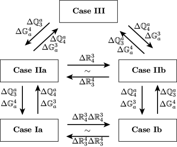
Figure 1: Schematic representation of the relations between the invariant subspaces. The opposite coproducts also respect the above diagram, as well as all their Yangian counterparts.

These relations between the different cases will play an important role in the derivation of the full S-matrix. In the next section we will introduce two different sets of bases which allow for a natural interpretation of the S-matrix. These bases will make use of the full Yangian symmetry rather than just the $\mathfrak{su}(2|2)$ as we did in this section. In this framework we can solve Case I. Then we employ the different arrows in Figure 1 (and their Yangian counterparts) to relate the different S-matrices to the Case I S-matrix.

Summarizing, we find that the S-matrix is of block-diagonal form

$${\mathbb{S}}=\begin{pmatrix}\framebox{\small{$\mathscr{X}$}}&~{}&~{}&~{}&~{}\\ ~{}&\framebox{\LARGE{$\mathscr{Y}$}}&~{}&\mbox{\Huge{$0$}}&~{}\\ ~{}&~{}&\framebox{\Huge{$\mathscr{Z}$}}&~{}&~{}\\ ~{}&\mbox{\Huge{$0$}}&~{}&\framebox{\LARGE{$\mathscr{Y}$}}&~{}\\ ~{}&~{}&~{}&~{}&\framebox{\small{$\mathscr{X}$}}\end{pmatrix}.$$ (27)

The outer blocks scatter states from $V^{\rm{I}}$

$$\mathscr{X}:V^{\rm{I}}\longrightarrow V^{\rm{I}}$$ (28)

$$|k,l\rangle^{\rm{I}}\mapsto\sum_{m=0}^{k+l}\mathscr{X}^{k,l}_{m}|m,k+l-m\rangle^{\rm{I}},$$ (29)

where $\mathscr{X}^{k,l}_{m}$ will be given by (4.1). The blocks $\mathscr{Y}$ describe the scattering of states from $V^{\rm{II}}$

$$\mathscr{Y}:V^{\rm{II}}\longrightarrow V^{\rm{II}}$$ (30)

$$|k,l\rangle^{\rm{II}}_{j}\mapsto\sum_{m=0}^{k+l}\sum_{j=1}^{4}\mathscr{Y}^{k,l;j}_{m;i}|m,k+l-m\rangle^{\rm{II}}_{j}.$$ (31)

These S-matrix elements are given in (111). Finally, the middle block deals with the third case

$$\mathscr{Z}:V^{\rm{III}}\longrightarrow V^{\rm{III}}$$ (32)

$$|k,l\rangle^{\rm{III}}_{j}\mapsto\sum_{m=0}^{k+l}\sum_{j=1}^{6}\mathscr{Z}^{k,l;j}_{m;i}|m,k+l-m\rangle^{\rm{III}}_{j},$$ (33)

with $\mathscr{Z}^{k,l;j}_{m;i}$ from (149).

We recall that the full ${\rm AdS}_{5}\times{\rm S}^{5}$ string bound state S-matrix is then obtained by taking two copies and multiplying each one of them with the phase factor [43]

$$S_{0}(p_{1},p_{2}) = \left(\frac{x_{1}^{-}}{x_{1}^{+}}\right)^{\frac{\ell_{2}}{2}}\left(\frac{x_{2}^{+}}{x_{2}^{-}}\right)^{\frac{\ell_{1}}{2}}\sigma(x_{1},x_{2})\times$$ (34)

$$\times\sqrt{G(\ell_{2}-\ell_{1})G(\ell_{2}+\ell_{1})}\prod_{q=1}^{\ell_{1}-1}G(\ell_{2}-\ell_{1}+2q),$$

where, in our conventions,

$$G(Q)=\frac{u_{1}-u_{2}+\frac{Q}{2}}{u_{1}-u_{2}-\frac{Q}{2}}$$ (35)

gives the standard pole at bound-state number $Q$ (see Section 4.2 later on for a discussion on the physical poles of the S-matrix). Here $u$ is given by

$$u \equiv \frac{g}{4i}\left(x^{+}+\frac{1}{x^{+}}+x^{-}+\frac{1}{x^{-}}\right).$$ (36)

3 Yangian Symmetry and Coproducts

So far we have only used $\mathfrak{su}(2|2)$ symmetry to study the bound state S-matrix. This, however, is not enough to fix the S-matrix (up to an overall phase). In particular, it was found that one needs to impose the Yang-Baxter equation by hand to attain this [43]. An alternative to this method was shown to come from Yangian symmetry [47].

The Yangian of $\mathfrak{su}(2|2)$ has a Hopf-algebra structure. In this language the invariance of the S-matrix can be formulated as

$${\mathbb{S}}~{}\Delta(\mathbb{J}^{A}) = \Delta^{op}(\mathbb{J}^{A})~{}{\mathbb{S}},$$

$${\mathbb{S}}~{}\Delta(\hat{\mathbb{J}}^{A}) = \Delta^{op}(\hat{\mathbb{J}}^{A})~{}{\mathbb{S}},$$ (37)

where $\hat{\mathbb{J}}$ stands for any generator of the Yangian. For explicit formulae and more details we refer to Appendix A. All this seems to indicate that the full Yangian of $\mathfrak{su}(2|2)$ should be viewed as the underlying symmetry algebra of scattering processes. Indeed, as we will see later on, we are able to construct any bound state S-matrix from this algebra.

3.1 (Opposite) coproduct basis

Let us turn back to the invariant subspaces. In this section, we define different bases for each case apart from the standard basis, which is commonly used in the literature. We call them the coproduct basis and the opposite coproduct basis. The basis transformation between the coproduct (opposite coproduct) basis and the standard one will be denoted by $\Lambda$ ($\Lambda^{op}$, respectively).

These bases will be constructed by using Yangian generators to create states out of a chosen vacuum. This is similar to [35] where it was used to study the Bethe Ansatz. We define our vacuum to be

$$|0\rangle\equiv w_{1}^{\ell_{1}}\ v_{1}^{\ell_{2}},$$ (38)

just as it is used in the coordinate Bethe Ansatz. We normalize our S-matrix in such a way that $\mathbb{S}|0\rangle=|0\rangle$. The (opposite) coproduct basis will consist of states created by the (opposite) coproducts of various symmetry generators acting on this vacuum. Clearly, the S-matrix has a natural interpretation in these bases, and can be formulated in terms of $\Lambda$ and $\Lambda^{op}$, as will be explained in section 3.2. We will now list the explicit formulae for the different bases.

Case I, $K^{\mathrm{II}}=2N+2,K^{\mathrm{III}}=N+2$.

The coproduct basis is given by

$$\Delta(\mathbb{Q}^{1}_{3})\Delta(\mathbb{G}_{2}^{4})\prod_{i=q+1}^{N}\Delta(\mathbb{L}^{1}_{2})\prod_{j=1}^{q}\Delta(\hat{\mathbb{L}}^{1}_{2})|0\rangle,\qquad q=0,1,\ldots N,$$ (39)

and the opposite coproduct basis is given by

$$\Delta^{op}(\mathbb{Q}^{1}_{3})\Delta^{op}(\mathbb{G}_{2}^{4})\prod_{i=k+1}^{N}\Delta^{op}(\mathbb{L}^{1}_{2})\prod_{j=1}^{k}\Delta^{op}(\hat{\mathbb{L}}^{1}_{2})|0\rangle,\qquad k=0,1,\ldots N.$$ (40)

Each of these two bases is indeed composed of $N+1$ different vectors. By explicitly working out the coproducts one can see that these vectors form a basis for Case I. One could also consider an alternative choice, like for instance

$$\Delta(\mathbb{Q}^{1}_{3})\Delta(\hat{\mathbb{Q}}^{1}_{3})\prod_{i=k+1}^{N}\Delta(\mathbb{L}^{1}_{2})\prod_{j=1}^{k}\Delta(\hat{\mathbb{L}}^{1}_{2})|0\rangle,$$ (41)

but these vectors are readily seen to be proportional to (39).

It is also straightforwardly seen why (39) actually describes Case I from the point of view of the quantum numbers $K^{\rm{II}},K^{\rm{III}}$. The operators $\Delta\mathbb{L}^{1}_{2},\Delta\hat{\mathbb{L}}^{1}_{2}$ create a boson of type $2$ out of the vacuum and the supersymmetry generators $\Delta\mathbb{Q}^{1}_{3},\Delta\hat{\mathbb{Q}}^{1}_{3}$ create a fermion of type $3$. Hence we find that $K^{\rm{II}}=2\#\mathbb{L}^{1}_{2}+2\#\Delta\hat{\mathbb{L}}^{1}_{2}+\#\Delta\mathbb{Q}^{1}_{3}+\#\Delta\hat{\mathbb{Q}}^{1}_{3}$ and $K^{\rm{III}}=\#\mathbb{L}^{1}_{2}+\#\Delta\hat{\mathbb{L}}^{1}_{2}+\#\Delta\mathbb{Q}^{1}_{3}+\#\Delta\hat{\mathbb{Q}}^{1}_{3}$. This indeed coincides with $K^{\mathrm{II}}=2N+2,K^{\mathrm{III}}=N+2$.

Case II, $K^{\mathrm{II}}=2N+1,K^{\mathrm{III}}=N+1$.

The coproduct basis is given by

$$\Delta(\mathbb{Q}^{1}_{3})\prod_{i=q+1}^{N}\Delta(\mathbb{L}^{1}_{2})\prod_{j=1}^{q}\Delta(\hat{\mathbb{L}}^{1}_{2})|0\rangle,$$

$$\Delta(\hat{\mathbb{Q}}^{1}_{3})\prod_{i=q+1}^{N}\Delta(\mathbb{L}^{1}_{2})\prod_{j=1}^{q}\Delta(\hat{\mathbb{L}}^{1}_{2})|0\rangle,$$

$$\Delta(\mathbb{Q}^{1}_{3})\Delta(\hat{\mathbb{Q}}^{1}_{3})\Delta(\mathbb{Q}^{1}_{4})\prod_{i=q+1}^{N-1}\Delta(\mathbb{L}^{1}_{2})\prod_{j=1}^{q}\Delta(\hat{\mathbb{L}}^{1}_{2})|0\rangle,$$

$$\Delta(\mathbb{Q}^{1}_{3})\Delta(\hat{\mathbb{Q}}^{1}_{3})\Delta(\hat{\mathbb{Q}}^{1}_{4})\prod_{i=q+1}^{N-1}\Delta(\mathbb{L}^{1}_{2})\prod_{j=1}^{q}\Delta(\hat{\mathbb{L}}^{1}_{2})|0\rangle,$$ (42)

and similar expressions hold for the opposite coproduct basis. One can again compute $K^{\rm{II}},K^{\rm{III}}$ for these states and see explicitly that they describe Case II.

Case III, $K^{\mathrm{II}}=2N,K^{\mathrm{III}}=N$.

The coproduct basis is

$$\prod_{i=q+1}^{N}\Delta(\mathbb{L}^{1}_{2})\prod_{j=1}^{q}\Delta(\hat{\mathbb{L}}^{1}_{2})|0\rangle,$$

$$\Delta(\mathbb{Q}^{1}_{3})\Delta(\mathbb{Q}^{1}_{4})\prod_{i=q+1}^{N-1}\Delta(\mathbb{L}^{1}_{2})\prod_{j=1}^{q}\Delta(\hat{\mathbb{L}}^{1}_{2})|0\rangle,$$

$$\Delta(\mathbb{Q}^{1}_{3})\Delta(\hat{\mathbb{Q}}^{1}_{4})\prod_{i=q+1}^{N-1}\Delta(\mathbb{L}^{1}_{2})\prod_{j=1}^{q}\Delta(\hat{\mathbb{L}}^{1}_{2})|0\rangle,$$

$$\Delta(\hat{\mathbb{Q}}^{1}_{3})\Delta(\mathbb{Q}^{1}_{4})\prod_{i=q+1}^{N-1}\Delta(\mathbb{L}^{1}_{2})\prod_{j=1}^{q}\Delta(\hat{\mathbb{L}}^{1}_{2})|0\rangle,$$

$$\Delta(\hat{\mathbb{Q}}^{1}_{3})\Delta(\hat{\mathbb{Q}}^{1}_{4})\prod_{i=q+1}^{N-1}\Delta(\mathbb{L}^{1}_{2})\prod_{j=1}^{q}\Delta(\hat{\mathbb{L}}^{1}_{2})|0\rangle,$$

$$\Delta(\mathbb{Q}^{1}_{3})\Delta(\mathbb{Q}^{1}_{4})\Delta(\hat{\mathbb{Q}}^{1}_{3})\Delta(\hat{\mathbb{Q}}^{1}_{4})\prod_{i=q+1}^{N-2}\Delta(\mathbb{L}^{1}_{2})\prod_{j=1}^{q}\Delta(\hat{\mathbb{L}}^{1}_{2})|0\rangle.$$

These are readily seen to be $6N$ states and their quantum numbers are of the form $K^{\mathrm{II}}=2N,K^{\mathrm{III}}=N$.

The Yangian generators also provide maps between the different cases. In particular, one finds that Figure 1 also holds for Yangian generators. One important thing to notice is the following. Even though, for example, $\Delta\mathbb{Q}^{2}_{3}$ maps Case II onto Case I, this does not automatically give a straightforward map between the vector spaces $V_{k,l}^{\rm{A}}$. For instance, one has

$$\Delta\mathbb{Q}^{2}_{3}:V_{k,l}^{\rm{II}}\longrightarrow V_{k,l-1}^{\rm{I}}\oplus V_{k-1,l}^{\rm{I}},$$ (43)

$$\Delta\hat{\mathbb{Q}}^{2}_{3}:V_{k,l}^{\rm{II}}\longrightarrow V_{k+1,l-1}^{\rm{I}}\oplus V_{k,l}^{\rm{I}}\oplus V_{k-1,l+1}^{\rm{I}}.$$ (44)

These relations between the different cases will be used later on.

3.2 S-matrix in coproduct basis

The fact that the coproduct basis is well suited for computing the S-matrix can be seen from (3). One sees that the S-matrix directly maps the coproduct basis onto the opposite coproduct basis. In particular, since we normalize the S-matrix in such a way that $\mathbb{S}|0\rangle=|0\rangle$, we see that the S-matrix, when written as a map between these two bases, is just the identity matrix.

In other words, one can now get the general formula for the S-matrix in the standard basis just by applying the appropriate basis transformations. Let us denote the S-matrix written in the standard basis as $\mathbb{S}$. One then finds:

$$\mathbb{S}=\Lambda^{op}\Lambda^{-1}.$$ (45)

Note that the explicit matrices $\Lambda$ and $\Lambda^{op}$ respectively, just consist of the coproduct vectors written in the standard basis. The above discussion can be summarized in the following commutative diagram:

$$\begin{CD}\{\rm{coproduct\ basis}\}@>{\mathbbm{1}}>{}>\{\rm{opposite\ coproduct\ basis}\}\\ @V{\Lambda}V{}V@V{\Lambda^{op}}V{}V\\ \{\rm{standard\ basis}\}@>{\mathbb{S}}>{}>\{\rm{standard\ basis}\}.\end{CD}$$ (46)

The computationally hard part is finding the explicit inverse of $\Lambda$. For any explicit case at hand this can be done by simple linear algebra, but the expressions become rather involved. However, we will be able to carry out this procedure in full generality for the S-matrix of Case I, and use this result to find the S-matrix for all the other states. To illustrate the above discussion, we conclude this section with an explicit example.

One of the easiest examples is that of $K^{\mathrm{II}}=1$, which can be considered as a warm-up for Case II. The vector space consisting of these states is only two dimensional. The standard basis vectors are

$$\theta_{3}w_{1}^{\ell_{1}-1}v_{1}^{\ell_{2}},\qquad w_{1}^{\ell_{1}}\vartheta_{3}v_{1}^{\ell_{2}-1}.$$ (47)

The coproduct basis is given by

$$\Delta(\mathbb{Q}^{1}_{3})|0\rangle,\qquad\Delta(\hat{\mathbb{Q}}^{1}_{3})|0\rangle.$$ (48)

Explicitly, when written down in terms of the standard basis, this gives:

$$\Delta(\mathbb{Q}^{1}_{3})|0\rangle = a_{1}\ell_{1}\theta_{3}w_{1}^{\ell_{1}-1}v_{1}^{\ell_{2}}+a_{2}\ell_{2}w_{1}^{\ell_{1}}\vartheta_{3}v_{1}^{\ell_{2}-1}$$

$$\Delta(\hat{\mathbb{Q}}^{1}_{3})|0\rangle = \frac{\ell_{1}\{\zeta a_{2}(a_{1}d_{2}-b_{2}c_{1})\ell_{2}-ia_{1}u_{1}\}}{2\zeta}\theta_{3}w_{1}^{\ell_{1}-1}v_{1}^{\ell_{2}}+$$

$$+\frac{\ell_{2}\{\zeta a_{1}(b_{1}c_{2}-a_{2}d_{1})\ell_{1}-ia_{2}u_{2}\}}{2\zeta}w_{1}^{\ell_{1}}\vartheta_{3}v_{1}^{\ell_{2}-1},$$

or, more conveniently written in matrix form,

$$\Lambda=\begin{pmatrix}a_{1}\ell_{1}~{}&~{}\frac{\ell_{1}\{\zeta a_{2}(a_{1}d_{2}-b_{2}c_{1})\ell_{2}-ia_{1}u_{1}\}}{2\zeta}\\ a_{2}\ell_{2}~{}&~{}\frac{\ell_{2}\{\zeta a_{1}(-a_{2}d_{1}+b_{1}c_{2})\ell_{1}-ia_{2}u_{2}\}}{2\zeta}\end{pmatrix}.$$ (50)

One obtains a similar expression for the basis transformation concerning $\Lambda^{op}$.

It is now an easy exercise to compute $\mathbb{S}$ for this case via (45). Doing the algebra gives the following result:

$$\mathbb{S}=\begin{pmatrix}e^{-i\frac{p_{2}}{2}}\frac{x^{+}_{1}-x^{+}_{2}}{x^{+}_{1}-x^{-}_{2}}~{}&~{}\frac{\sqrt{\ell_{1}}\eta(p_{1})}{\sqrt{\ell_{2}}\eta(p_{2})}\frac{x^{+}_{2}-x^{-}_{2}}{x^{+}_{1}-x^{-}_{2}}\\ \frac{e^{i\frac{p_{1}}{2}}}{e^{i\frac{p_{2}}{2}}}\frac{\sqrt{\ell_{2}}\eta(p_{2})}{\sqrt{\ell_{1}}\eta(p_{1})}\frac{x^{+}_{1}-x^{-}_{1}}{x^{+}_{1}-x^{-}_{2}}~{}&~{}e^{i\frac{p_{1}}{2}}\frac{x^{-}_{1}-x^{-}_{2}}{x^{+}_{1}-x^{-}_{2}}\end{pmatrix},$$ (51)

which indeed coincides with the known S-matrices [6, 15, 43, 31], and also with the coefficients recently found in [35].

4 Complete Solution of Case I

In this section, we will discuss the S-matrix of Case I . We will use Yangian symmetry to derive its explicit form. This S-matrix proves to be the building block out of which the S-matrices for both Case II and Case III can be constructed. Because of this, we will study it in detail before moving on to the other cases. We will analyze its pole structure and also compare this S-matrix in the semi-classical limit to the classical $r$-matrix proposed in [52].

4.1 Explicit solution

Our starting point is the coproduct basis (39). It is convenient to reorder the products in the following way:

$$\left\{\prod_{i=q+1}^{N}\Delta(\mathbb{L}^{1}_{2})\prod_{j=1}^{q}\Delta(\hat{\mathbb{L}}^{1}_{2})\right\}\Delta(\mathbb{Q}^{1}_{3})\Delta(\mathbb{G}^{4}_{2})|0\rangle.$$ (52)

The action of the susy generators on the vacuum is of the form

$$\Delta(\mathbb{Q}^{1}_{3})\Delta(\mathbb{G}^{4}_{2})|0\rangle=(a_{2}c_{1}-a_{1}c_{2})\ell_{1}\ell_{2}|0,0\rangle^{\rm{I}},$$ (53)

with a similar expression for the opposite version. As a matter of fact, from this one can straightforwardly read off the action of the S-matrix on $|0,0\rangle^{\rm{I}}$:

$$\mathbb{S}|0,0\rangle^{\rm{I}} = \frac{\mathbb{S}\Delta(\mathbb{Q}^{1}_{3})\Delta(\mathbb{G}^{4}_{2})|0\rangle}{(a_{2}c_{1}-a_{1}c_{2})\ell_{1}\ell_{2}}$$ (54)

$$= \frac{\Delta^{op}(\mathbb{Q}^{1}_{3})\Delta^{op}(\mathbb{G}^{4}_{2})\mathbb{S}|0\rangle}{(a_{2}c_{1}-a_{1}c_{2})\ell_{1}\ell_{2}}$$

$$= \frac{a_{4}c_{3}-a_{3}c_{4}}{a_{2}c_{1}-a_{1}c_{2}}|0,0\rangle^{\rm{I}}.$$

In other words, the S-matrix multiplies $|0,0\rangle^{\rm{I}}$ by a scalar. We will denote this scalar by $D$. In terms of $x^{\pm}$, it is given by

$$D\equiv\frac{a_{4}c_{3}-a_{3}c_{4}}{a_{2}c_{1}-a_{1}c_{2}}=\frac{x_{1}^{-}-x_{2}^{+}}{x_{1}^{+}-x_{2}^{-}}\frac{e^{i\frac{p_{1}}{2}}}{e^{i\frac{p_{2}}{2}}}.$$ (55)

It is readily seen that this coefficient is indeed consistent with the action of the S-matrices previously found in [6, 15, 43, 31].

One can now use the generators $\mathbb{L}^{1}_{2},\hat{\mathbb{L}}^{1}_{2}$ to construct a generic Case I state $|k,l\rangle^{\rm{I}}$ from $|0,0\rangle^{\rm{I}}$, for arbitrary $k,l$. This can be seen by considering the following identities:

$$(\mathbb{L}^{1}_{2}\otimes\mathbbm{1})(\delta u+\Delta(\mathbb{L}^{1}_{1}))|k,l\rangle^{\rm{I}} = \left\{\Delta(\hat{\mathbb{L}}^{1}_{2})-u_{2}\Delta(\mathbb{L}^{1}_{2})+\Delta(\mathbb{L}^{1}_{2})\circ(\mathbb{L}^{1}_{1}\otimes\mathbbm{1})\right\}|k,l\rangle^{\rm{I}},$$ (56)

$$(\mathbbm{1}\otimes\mathbb{L}^{1}_{2})(\delta u+\Delta(\mathbb{L}^{1}_{1}))|k,l\rangle^{\rm{I}} = -\left\{\Delta(\hat{\mathbb{L}}^{1}_{2})-u_{1}\Delta(\mathbb{L}^{1}_{2})-\Delta(\mathbb{L}^{1}_{2})\circ(\mathbbm{1}\otimes\mathbb{L}^{1}_{1})\right\}|k,l\rangle^{\rm{I}},$$

where

$$\delta u=u_{1}-u_{2}.$$ (57)

Since $\Delta(\mathbb{L}^{1}_{1})|k,l\rangle^{\rm{I}}=\frac{\ell_{1}+\ell_{2}-2(k+l+1)}{2}|k,l\rangle^{\rm{I}}$, it is obvious that the left hand side is proportional to $|k+1,l\rangle$ and $|k,l+1\rangle$ respectively. By applying these operators inductively to $|0,0\rangle$, one finds

$$\left\{\prod_{m=1}^{k}(\ell_{1}-m)\prod_{n=1}^{l}(\ell_{2}-n)\prod_{q=1}^{k+l}\left(\delta u+\frac{\ell_{1}+\ell_{2}}{2}-q\right)\right\}|k,l\rangle=$$

$$\qquad\left[(\mathbb{L}^{1}_{2}\otimes\mathbbm{1})(\delta u+\Delta(\mathbb{L}^{1}_{1}))\right]^{k}\left[(\mathbbm{1}\otimes\mathbb{L}^{1}_{2})(\delta u+\Delta(\mathbb{L}^{1}_{1}))\right]^{l}|0,0\rangle.$$ (58)

Then, by (56),

$$|k,l\rangle^{\rm{I}}=$$ (59)

$$\quad\ \ \ \frac{\prod_{i=1}^{k}\left[\Delta(\hat{\mathbb{L}}^{1}_{2})+\frac{\ell_{1}-2u_{2}-2i+1}{2}\Delta(\mathbb{L}^{1}_{2})\right]\prod_{j=1}^{l}\left[-\Delta(\hat{\mathbb{L}}^{1}_{2})-\frac{1+2j-2u_{1}-\ell_{2}}{2}\Delta(\mathbb{L}^{1}_{2})\right]}{\prod_{m=1}^{k}(\ell_{1}-m)\prod_{n=1}^{l}(\ell_{2}-n)\prod_{q=1}^{k+l}\left(\delta u+\frac{\ell_{1}+\ell_{2}}{2}-q\right)}|0,0\rangle^{\rm{I}}.$$

This exactly tells us how to write a state in the standard basis as a combination of coproducts. In other words, this explicitly indicates how to construct $\Lambda^{-1}$. It is now straightforward to obtain the action of the S-matrix on Case I states from this. The symmetry properties of the S-matrix, together with (54), now imply

$$\mathbb{S}|k,l\rangle^{\rm{I}}=$$ (60)

$$\ \ D\frac{\prod_{i=1}^{k}\left[\Delta^{op}(\hat{\mathbb{L}}^{1}_{2})-\frac{2u_{2}-\ell_{1}+2i-1}{2}\Delta^{op}(\mathbb{L}^{1}_{2})\right]\prod_{j=1}^{l}\left[\frac{2u_{1}+\ell_{2}-1-2j}{2}\Delta^{op}(\mathbb{L}^{1}_{2})-\Delta^{op}(\hat{\mathbb{L}}^{1}_{2})\right]}{\prod_{m=1}^{k}(\ell_{1}-m)\prod_{n=1}^{l}(\ell_{2}-n)\prod_{q=1}^{k+l}\left(\delta u+\frac{\ell_{1}+\ell_{2}}{2}-q\right)}|0,0\rangle^{\rm{I}}.$$

The right hand side can be computed straightforwardly. One finds that $\mathbb{S}|k,l\rangle^{\rm{I}}$ is of the form

$$\mathbb{S}|k,l\rangle^{\rm{I}}=\sum_{n=0}^{k+l}\mathscr{X}^{k,l}_{n}|n,k+l-n\rangle^{\rm{I}},$$ (61)

with

$$\mathscr{X}^{k,l}_{n} = D\frac{\prod_{i=1}^{n}(\ell_{1}-i)\prod_{i=1}^{k+l-n}(\ell_{2}-i)}{\prod_{p=1}^{k}(\ell_{1}-p)\prod_{p=1}^{l}(\ell_{2}-p)\prod_{p=1}^{k+l}(\delta u+\frac{\ell_{1}+\ell_{2}}{2}-p)}\times$$

$$\times\sum_{m=0}^{k}\left\{{k\choose k-m}{l\choose n-m}\prod_{p=1}^{m}\mathfrak{c}^{+}_{p}\prod_{p=1-m}^{l-n}\mathfrak{c}^{-}_{p}\prod_{p=1}^{k-m}\mathfrak{d}_{\frac{k-p+2}{2}}\prod_{p=1}^{n-m}\tilde{\mathfrak{d}}_{\frac{k+l-m-p+2}{2}}\right\}.$$

The coefficients are given by

$$\mathfrak{c}^{\pm}_{m} = \delta u\pm\frac{\ell_{1}-\ell_{2}}{2}-m+1,$$

$$\tilde{\mathfrak{c}}^{\pm}_{m} = \delta u\pm\frac{\ell_{1}+\ell_{2}}{2}-m+1,$$ (63)

$$\mathfrak{d}_{i} = \ell_{1}+1-2i,$$

$$\tilde{\mathfrak{d}}_{i} = \ell_{2}+1-2i.$$

It is worthwhile to note that in the special case $l=0$ (and similarly for $k=0$) this expression reduces considerably. For later use, we can write it in the following way:

$$\mathscr{X}^{k,0}_{k-n}=D{k\choose n}\frac{\prod_{p=1}^{n}(\ell_{2}-p)\prod_{p=1}^{k-n}(\delta u+\frac{\ell_{1}-\ell_{2}}{2}-p+1)}{\prod_{p=1}^{k}(\delta u+\frac{\ell_{1}+\ell_{2}}{2}-p)}.$$ (64)

In all of the above expressions it is understood that products are set to 1 whenever they run over negative integers, i.e. $\prod_{a}^{b}=1$ if $b<a$, and the binomial ${x\choose y}$ is taken to be zero if $y>x$ and if $y<0$.

We can notice how the formula we have found bears a rational dependence on the difference of the spectral parameters, as typical of Yangian universal R-matrices in evaluation representations. The following function, meromorphic in all the parameters, coincides with (4.1) in the appropriate domain of integer values:

$$\mathscr{X}^{k,l}_{n} = (-1)^{k+n}\,\pi D\frac{\sin[(k-\ell_{1})\pi]\,\Gamma(l+1)}{\sin[\ell_{1}\pi]\sin[(k+l-\ell_{2}-n)\pi]\,\Gamma(l-\ell_{2}+1)\Gamma(n+1)}\times$$

$$\frac{\Gamma(n+1-\ell_{1})\Gamma\left(l+\frac{\ell_{1}-\ell_{2}}{2}-n-\delta u\right)\Gamma\left(1-\frac{\ell_{1}+\ell_{2}}{2}-\delta u\right)}{\Gamma\left(k+l-\frac{\ell_{1}+\ell_{2}}{2}-\delta u+1\right)\Gamma\left(\frac{\ell_{1}-\ell_{2}}{2}-\delta u\right)}\times$$

$${}_{4}\tilde{F}_{3}\left(-k,-n,\delta u+1-\frac{\ell_{1}-\ell_{2}}{2},\frac{\ell_{2}-\ell_{1}}{2}-\delta u;1-\ell_{1},\ell_{2}-k-l,l-n+1;1\right),$$

where one has defined ${}_{4}\tilde{F}_{3}(x,y,z,t;r,v,w;\tau)={{}_{4}F_{3}}(x,y,z,t;r,v,w;\tau)/[\Gamma(r)\Gamma(v)\Gamma(w)]$.

Moreover, we can easily see that we are in a special situation, since the parameters entering the hypergeometric function ${}_{4}F_{3}(a_{1},a_{2},a_{3},a_{4};b_{1},b_{2},b_{3};1)$ satisfy $\sum_{i=1}^{4}a_{i}-\sum_{j=1}^{3}b_{j}=-1$. When this happens, the hypergeometric function reduces to a $6j$-symbol, according to the following formula (see for example [56]):

$${}_{4}F_{3}\left(a_{1},a_{2},a_{3},a_{4};b_{1},b_{2},b_{3};1\right)=\frac{(-1)^{b_{1}+1}\Gamma\left(b_{2}\right)\Gamma\left(b_{3}\right)\sqrt{\Gamma\left(1-a_{1}\right)\Gamma\left(1-a_{2}\right)\Gamma\left(1-a_{3}\right)}}{\Gamma\left(1-b_{1}\right)\sqrt{\Gamma\left(b_{2}-a_{1}\right)\Gamma\left(b_{2}-a_{2}\right)}}\times$$ (68)

$$\qquad\frac{\sqrt{\Gamma\left(1-a_{4}\right)\Gamma\left(a_{1}-b_{1}+1\right)\Gamma\left(a_{2}-b_{1}+1\right)\Gamma\left(a_{3}-b_{1}+1\right)\Gamma\left(a_{4}-b_{1}+1\right)}}{\sqrt{\Gamma\left(b_{2}-a_{3}\right)\Gamma\left(b_{2}-a_{4}\right)\Gamma\left(b_{3}-a_{1}\right)\Gamma\left(b_{3}-a_{2}\right)\Gamma\left(b_{3}-a_{3}\right)\Gamma\left(b_{3}-a_{4}\right)}}\times$$

$$\qquad\,\,\left\{\begin{array}[]{ccc}\frac{1}{2}\left(-a_{1}-a_{4}+b_{3}-1\right)&\frac{1}{2}\left(-a_{1}-a_{3}+b_{2}-1\right)&\frac{1}{2}\left(a_{1}+a_{2}-b_{1}-1\right)\\ \frac{1}{2}\left(-a_{2}-a_{3}+b_{3}-1\right)&\frac{1}{2}\left(-a_{2}-a_{4}+b_{2}-1\right)&\frac{1}{2}\left(a_{3}+a_{4}-b_{1}-1\right)\end{array}\right\}.$$

By identifying the parameters we see that the relevant $6j$-symbol

$$\left\{\begin{array}[]{ccc}j_{1}&j_{2}&j_{3}\\ j_{4}&j_{5}&j_{6}\end{array}\right\}$$ (71)

has coefficients

$$j_{1}=\frac{1}{2}\left(k+l-n+\frac{\ell_{1}-\ell_{2}}{2}+\delta u\right),$$

$$j_{2}=\frac{1}{2}\left(\frac{\ell_{1}+\ell_{2}}{2}-2-l-\delta u\right),$$

$$j_{3}=\frac{1}{2}\left(\ell_{1}-2-k-n\right),$$

$$j_{4}=\frac{1}{2}\left(\frac{\ell_{1}-\ell_{2}}{2}-1+l-\delta u\right),$$

$$j_{5}=\frac{1}{2}\left(\frac{\ell_{1}+\ell_{2}}{2}-1-k-l+n+\delta u\right),$$

$$j_{6}=\frac{1}{2}\left(\ell_{2}-1\right).$$ (72)

For generic values of $\delta u$, the $6j$-symbol is understood in the same sense as in the comment above formula (4.1). However, one can prove that, for values of $\delta u$ corresponding to the physical poles (see also the discussion below), the entries of the $6j$-symbol are indeed half-integer, as one may expect from the fusion rules of $\mathfrak{su}(2)$ representations.

In the special case $l=0$ (a similar argument would hold for $k=0$), we can go back to expression (4.1), and see that it can be casted in the following form:

$$\mathscr{X}^{k,0}_{k-n}=D\frac{\Gamma(k+1)\Gamma(1+n-\ell_{2})\Gamma\left(1-\frac{\ell_{1}+\ell_{2}}{2}-\delta u\right)\Gamma\left(k+\frac{\ell_{2}}{2}-\frac{\ell_{1}}{2}-n-\delta u\right)}{\Gamma(1-\ell_{2})\Gamma(k-n+1)\Gamma(n+1)\,\Gamma\left(k-\frac{\ell_{1}+\ell_{2}}{2}-\delta u+1\right)\Gamma\left(\frac{\ell_{2}-\ell_{1}}{2}-\delta u\right)}.$$

4.2 Poles

Next, we will analyze the pole structure of formula (4.1). For simplicity, we will restrict to the special case of expression (64) in this section. The general case will then be analyzed in Appendix B.

For the remainder of this section, we rescale the coupling constant and the spectral parameters according to $g\rightarrow g\sqrt{2}$, $u\rightarrow\frac{g}{i\sqrt{2}}u$, in order to adapt our conventions to those of [48]. Formula (64) becomes

$$\mathscr{X}^{k,0}_{k-n}=D{k\choose n}\frac{\prod_{p^{\prime}=1}^{n}(\ell_{2}-p^{\prime})\prod_{q=1}^{k-n}(\delta u-\frac{i}{g\sqrt{2}}[2q-\ell_{1}+\ell_{2}-2])}{\prod_{p=1}^{k}(\delta u-\frac{i}{g\sqrt{2}}[2p-\ell_{1}-\ell_{2}])}.$$ (73)

We can recognize, following [48], the presence of potential poles of this formula at bound-state rank $2p-\ell_{1}-\ell_{2}$, which we now want to study. To begin with, in order for these poles to be ‘physical’ (namely, with a positive bound-state rank), one must have $2p\geq\ell_{1}+\ell_{2}$ (inclusion of the “equal” case will not affect the result). Since $p$ is at most as large as $k$, and, from the definition (61), $\ell_{1}\geq k+1$, we conclude that one needs $\ell_{1}\geq\ell_{2}+2$ and $2\ell_{1}-2\geq 2k\geq\ell_{1}+\ell_{2}$. If this holds, then the physical poles occur for the values of $k\geq p\geq(\ell_{1}+\ell_{2})/2$. There are two possibilities, which we analyze in what follows.

• The numerator does not identically vanish, and does not have zeroes for any physical values of the spectral parameters. This situation would leave physical poles uncancelled in the denominator. This happens if  $\ell_{2}\geq n+1$ (by looking at the product $\prod_{p^{\prime}=1}^{n}(\ell_{2}-p^{\prime})$), and if  $\ell_{1}-\ell_{2}\geq 2(k-n)$, with $k\geq n$ from (61). Combining the two conditions, we obtain $k\leq n+[(\ell_{1}-\ell_{2})/2]\leq-1+[(\ell_{1}+\ell_{2})/2]$, which contradicts the original condition for physical poles given above. Therefore, this situation cannot occur.

• The numerator does not identically vanish, but it has zeroes at some physical values of the spectral parameters. The latter can potentially cancel some of the physical poles, and we want to see whether few poles will be left uncancelled, or all of them will be neutralized. In order to have zeroes at physical values, we need $\ell_{1}-\ell_{2}\leq 2(k-n)-1$. This means that the interesting zeroes will occur at positive bound-state ranks running from $0$ up to $-k+[(\ell_{1}+\ell_{2})/2]$, while the interesting poles occur at bound-state ranks running from $0$ up to $n-k+1+[(\ell_{1}-\ell_{2})/2]$. But we see that the number of these zeroes is always larger than the number of physical poles. In fact, if one subtracts the two numbers, one gets $\ell_{2}-n-1$, which is bigger than (or at least equal to) zero in order for the amplitude not to identically vanish (once again, by looking at the product $\prod_{p^{\prime}=1}^{n}(\ell_{2}-p^{\prime})$). Therefore, also this second situation cannot occur, and we conclude that we cannot have physical poles in formula (64).

The result of this section and of Appendix B is consistent with the fact that in the $\mathfrak{su}(1|1)$ sector corresponding to Case I, one does not expect any physical bound-state poles [48, 16]. The factor of $D$ in fact cancels the s-channel pole at bound-state rank $\ell_{1}+\ell_{2}$ coming from the overall scalar factor, and no physical poles are left in this amplitude.

4.3 The classical limit

In this section, we want to take the classical limit [57] of the S-matrix for scattering of arbitrary states belonging to Case I, and show that it is reproduced by the universal formula given in [52]. For general transition amplitudes, though only in the situation where one has at most two bound-state components, this test has already been performed in [47].

When looking at formula (4.1), one can see that, besides expanding the factor $D$, one needs to expand the remaining expression, depending only on the difference $\delta u$ of the spectral parameters, for large values of $\delta u$. In the classical (near BMN) limit, in fact, the coupling $g$ goes to infinity. With our conventions (36), the spectral parameter $u$ grows linearly with $g$ in this regime, while both parameters $x^{\pm}$, expressed as

$$x^{\pm}_{i} = x_{i}\left(\sqrt{1-\frac{(\ell_{i}/g)^{2}}{(x_{i}-\frac{1}{x_{i}})^{2}}}\pm\frac{i\ell_{i}/g}{x_{i}-\frac{1}{x_{i}}}\right),$$ (74)

tend to their common classical value $x$ [58].

The relevant terms to the classical limit of (4.1) are given by the following expansion:

$$\mathscr{X}^{k,l}_{n} \sim (1+D_{cl})\frac{\bigg{(}1-\frac{1}{\delta u}\sum_{p=1}^{k+l}(\frac{\ell_{1}+\ell_{2}}{2}-p)\bigg{)}\,\prod_{i=1}^{n}(\ell_{1}-i)\prod_{i=1}^{k+l-n}(\ell_{2}-i)}{\prod_{p=1}^{k}(\ell_{1}-p)\prod_{p=1}^{l}(\ell_{2}-p)}\times$$ (75)

$$\times\sum_{m=0}^{k}\Bigg{\{}\bigg{(}1+\frac{1}{\delta u}\,\sum_{p=1}^{m}(\frac{\ell_{1}-\ell_{2}}{2}+1-p)+\frac{1}{\delta u}\sum_{p=1-m}^{l-n}(\frac{\ell_{2}-\ell_{1}}{2}+1-p)\bigg{)}\times$$

$$\,\times{\delta u}^{2m-k-n}\,{k\choose k-m}{l\choose n-m}\prod_{p=1}^{k-m}\mathfrak{d}_{\frac{k-p+2}{2}}\prod_{p=1}^{n-m}\tilde{\mathfrak{d}}_{\frac{k+l-m-p+2}{2}}\Bigg{\}},$$

where $D_{cl}$ denotes the first order in $1/g$ of $D$. Here, we have used the fact that the binomials enforce $l\geq n-m$, in order to obtain the power of ${\delta u}^{2m-k-n}$. Let us start by considering non-diagonal amplitudes, namely, $n$ different from $k$ (cfr. (61)). In order to do that, let us first reduce the above formula for the case $n\geq k$. In this case, the leading piece in the above expression is given by the term in the sum with $m=k$ (the binomials are in this case non-zero, since, from (61), one has $l\geq n-k$). The amplitude tends to

$$\mathscr{X}^{k,l}_{n} \sim \frac{1}{{\delta u}^{n-k}}\,\frac{\prod_{i=1}^{n}(\ell_{1}-i)\prod_{i=1}^{k+l-n}(\ell_{2}-i)}{\prod_{p=1}^{k}(\ell_{1}-p)\prod_{p=1}^{l}(\ell_{2}-p)}\,{l\choose n-k}\prod_{p=1}^{n-k}\tilde{\mathfrak{d}}_{\frac{l-p+2}{2}}.$$ (76)

As one can see, in the non-diagonal case only one of these amplitudes actually contributes to the classical limit (corresponding to the order $1/g$ of the scattering matrix). Namely, only the transition from a state characterized by quantum number $k$ to one with corresponding quantum number $n=k+1$ has the right order, the other ones being suppressed by higher powers of $\delta u$. In this situation, the classical amplitudes reads

$$\mathscr{X}^{k,l}_{k+1} \sim \frac{1}{{\delta u}}\,l(\ell_{1}-k-1).$$ (77)

We checked that this is exactly the value one gets from applying the universal formula of [52] to this amplitude. For convenience of the reader, we report here below their classical r-matrix.

$$r_{12} = \frac{\mathcal{T}_{12}-\Sigma\otimes\mathbb{H}-\mathbb{H}\otimes\Sigma}{i(u_{1}-u_{2})}-\frac{\Sigma\otimes\mathbb{H}}{iu_{2}}+\frac{\mathbb{H}\otimes\Sigma}{iu_{1}}+\frac{i}{2}(u_{2}^{-1}-u_{1}^{-1})\mathbb{H}\otimes\mathbb{H},$$ (78)

with

$$\mathcal{T}_{12}=2\left(\mathbb{R}^{\ \alpha}_{\beta}\otimes\mathbb{R}^{\ \beta}_{\alpha}-\mathbb{L}^{\ a}_{b}\otimes\mathbb{L}^{\ b}_{a}+\mathbb{G}^{\ \alpha}_{a}\otimes\mathbb{Q}^{\ a}_{\alpha}-\mathbb{Q}^{\ a}_{\alpha}\otimes\mathbb{G}^{\ \alpha}_{a}\right)$$ (79)

and

$$\Sigma=\frac{1}{2}\frac{1}{ad+bc}\left(w_{a}\frac{\partial}{\partial w_{a}}-\theta_{a}\frac{\partial}{\partial\theta_{\alpha}}\right).$$ (80)

In (78), we understand all generators (taken at their classical value) as differential operators, acting on the appropriate monomials corresponding to Case I states. We then compare the result with the expression we have found above for the first order in $1/g$ of the complete S-matrix.

Next, let us consider $k\geq n$. In this case the binomials force the leading piece in the sum to be the one with $m=n$. This reads (quite symmetrically w.r.t the previous case)

$$\mathscr{X}^{k,l}_{n} \sim \frac{1}{{\delta u}^{k-n}}\,\frac{\prod_{i=1}^{n}(\ell_{1}-i)\prod_{i=1}^{k+l-n}(\ell_{2}-i)}{\prod_{p=1}^{k}(\ell_{1}-p)\prod_{p=1}^{l}(\ell_{2}-p)}\,{k\choose k-n}\prod_{p=1}^{k-n}\mathfrak{d}_{\frac{k-p+2}{2}}.$$ (81)

Analogously, only one of the non-diagonal terms has the right falloff to be able to contribute to the classical r-matrix, namely the amplitude for quantum numbers $k$ to $n=k-1$. The contribution is given by

$$\mathscr{X}^{k,l}_{k-1} \sim \frac{1}{{\delta u}}\,k(\ell_{2}-l-1),$$ (82)

and we also checked it against the classical proposal of [52].

The diagonal part, for $n=k$, is slightly more complicated. The leading term can be obtained by specializing to $k=n$ either of the two formulas (76) or (81), and is easily seen to be equal to $1$, as expected. The quantum R-matrix goes in fact to the identity in the strict classical limit. The next to leading term of order $1/\delta u$ contributes to the classical r-matrix, and can be straightforwardly obtained from (75) as

$$\mathscr{X}^{k,l}_{k}-1 \sim D_{cl}\,+\frac{1}{{\delta u}}\Bigg{[}\sum_{p=1}^{k+l}(\frac{\ell_{1}+\ell_{2}}{2}-p)+\sum_{p=1}^{k}(\frac{\ell_{1}-\ell_{2}}{2}+1-p)+\sum_{p=1-k}^{l-k}(\frac{\ell_{2}-\ell_{1}}{2}+1-p)\Bigg{]}.$$

This expression can be explicitly evaluated, and, after supplementing it with the suitable overall scalar factor (cfr. [47]), we have checked that it precisely corresponds to the result coming from the universal formula of [52].

As a curiosity, we have checked that the order ${\cal{O}}(1/{g^{2}})$ of the Case I amplitude is completely reproduced by half the square of the classical r-matrix. The departure from a simple exponential series seems to reveal itself starting from the next order ${\cal{O}}(1/{g^{3}})$. We plan to come back to this issue in the future, in the light of possible consequences for the abstract form of the universal R-matrix (cf. for instance [59, 60]).

5 The S-matrix for Case II

In this section, we will use the S-matrix derived for Case I to find the S-matrix for Case II.

As explained in the previous sections, $\Delta\mathbb{Q}^{1}_{3},\Delta\mathbb{G}^{4}_{2}$ and their Yangian partners map Case II states onto Case I states. We introduce the Case II S-matrix in the following way

$$\mathbb{S}|k,l\rangle^{\rm{II}}_{i}=\sum_{j=1}^{4}\sum_{m=0}^{k+l}\mathscr{Y}^{k,l;j}_{m;i}|m,N-m\rangle^{\rm{II}}_{j},$$ (83)

where again $N=k+l$. This means that the coefficients $\mathscr{Y}^{k,l;j}_{m;i}$ actually correspond to the S-matrix restricted to the following spaces

$$\mathscr{Y}^{k,l;j}_{n;i}:V^{\rm{II}}_{k,l}\longrightarrow V^{\rm{II}}_{n,N-n}.$$ (84)

Generically, both spaces are 4 dimensional, and $\mathscr{Y}^{k,l;j}_{m;i}$ correspond to the coefficients of a $4\times 4$ matrix. One might wonder what happens for $n=0,N$ since e.g. $|0,N\rangle^{\rm{II}}_{4}$, strictly speaking, does not exist. However, it turns out that these states are always multiplied by 0. Hence, the $4\times 4$ matrix actually contains the non-generic case in which $n=0,N$. This will be explained later on in Section 7 and we will continue with deriving the generic $4\times 4$ matrix.

By now considering the action of $\Delta^{op}\mathbb{Q}^{1}_{3}$, we can relate the Case II S-matrix to (4.1). It is easily checked that

$$\Delta\mathbb{Q}^{1}_{3}|k,l\rangle^{\rm{II}}_{j}=Q_{j}(k,l)|k,l\rangle^{\rm{I}},$$ (85)

with

$$\begin{array}[]{lll}Q_{1}(k,l)=a_{2}(l-\ell_{2}),&&Q_{2}(k,l)=a_{1}(\ell_{1}-k),\\ Q_{3}(k,l)=b_{2},&&Q_{4}(k,l)=-b_{1}.\end{array}$$ (88)

Similar expressions are of course obtained for $\Delta^{op}\mathbb{Q}^{1}_{3},\Delta^{op}\mathbb{G}^{4}_{2},\Delta\mathbb{G}^{4}_{2}$. We can now apply our general strategy in the following fashion:

$${}^{\rm{I}}\langle n,N-n|~{}\Delta^{op}\mathbb{Q}^{1}_{3}\mathbb{S}~{}|k,l\rangle^{\rm{II}}_{i} = \sum_{j=1}^{4}\sum_{m=0}^{k+l}\mathscr{Y}^{k,l;j}_{m;i}\ {}^{\rm{I}}\langle n,N-n|~{}\Delta^{op}\mathbb{Q}^{1}_{3}~{}|m,N-m\rangle^{\rm{II}}_{j}$$ (89)

$$= \sum_{j=1}^{4}\sum_{m=0}^{k+l}\mathscr{Y}^{k,l;j}_{m;i}Q^{op}_{j}(m,N-m)\ ^{\rm{I}}\langle n,N-n|m,N-m\rangle^{\rm{I}}$$

$$= \sum_{j=1}^{4}\mathscr{Y}^{k,l;j}_{n;i}Q^{op}_{j}(n,N-n).$$

On the other hand, we can use the symmetry properties of the S-matrix to obtain

$${}^{\rm{I}}\langle n,N-n|~{}\Delta^{op}\mathbb{Q}^{1}_{3}\mathbb{S}~{}|k,l\rangle^{\rm{II}}_{i} = {}^{\rm{I}}\langle n,N-n|~{}\mathbb{S}\Delta\mathbb{Q}^{1}_{3}~{}|k,l\rangle^{\rm{II}}_{i}$$ (90)

$$= Q_{i}(k,l)^{\rm{I}}\langle n,N-n|~{}\mathbb{S}~{}|k,l\rangle^{\rm{II}}$$

$$= Q_{i}(k,l)\sum_{m=0}^{N}\mathscr{X}^{k,l}_{m}\ {}^{\rm{I}}\langle n,N-n|m,N-m\rangle^{\rm{I}}$$

$$= Q_{i}(k,l)\mathscr{X}^{k,l}_{n}.$$

Clearly, this gives us four linear equations relating the two S-matrices. A similar computation can be worked out using $\Delta^{op}\mathbb{G}_{2}^{4}$, giving four additional equations. We can cast the above formulae in a convenient matrix form:

$$\begin{pmatrix}\scriptstyle{a_{4}(N-n-\ell_{2})}&\scriptstyle{a_{3}(\ell_{1}-n)}&\scriptstyle{b_{4}}&\scriptstyle{-b_{3}}\\ \scriptstyle{c_{4}(N-n-\ell_{2})}&\scriptstyle{c_{3}(\ell_{1}-n)}&\scriptstyle{d_{4}}&\scriptstyle{-d_{3}}\\ \end{pmatrix}\mathscr{Y}^{k,l}_{n}=\mathscr{X}^{k,l}_{n}\begin{pmatrix}\scriptstyle{a_{2}(l-\ell_{2})}&\scriptstyle{a_{1}(\ell_{1}-k)}&\scriptstyle{b_{2}}&\scriptstyle{-b_{1}}\\ \scriptstyle{c_{2}(l-\ell_{2})}&\scriptstyle{c_{1}(\ell_{1}-k)}&\scriptstyle{d_{2}}&\scriptstyle{-d_{1}}\\ \end{pmatrix},$$ (91)

with

$$\mathscr{Y}^{k,l}_{n} \equiv \begin{pmatrix}\scriptstyle{\mathscr{Y}^{k,l;1}_{n;1}}&\scriptstyle{\mathscr{Y}^{k,l;1}_{n;2}}&\scriptstyle{\mathscr{Y}^{k,l;1}_{n;3}}&\scriptstyle{\mathscr{Y}^{k,l;1}_{n;4}}\\ \scriptstyle{\mathscr{Y}^{k,l;2}_{n;1}}&\scriptstyle{\mathscr{Y}^{k,l;2}_{n;2}}&\scriptstyle{\mathscr{Y}^{k,l;2}_{n;3}}&\scriptstyle{\mathscr{Y}^{k,l;2}_{n;4}}\\ \scriptstyle{\mathscr{Y}^{k,l;3}_{n;1}}&\scriptstyle{\mathscr{Y}^{k,l;3}_{n;2}}&\scriptstyle{\mathscr{Y}^{k,l;3}_{n;3}}&\scriptstyle{\mathscr{Y}^{k,l;3}_{n;4}}\\ \scriptstyle{\mathscr{Y}^{k,l;4}_{n;1}}&\scriptstyle{\mathscr{Y}^{k,l;4}_{n;2}}&\scriptstyle{\mathscr{Y}^{k,l;4}_{n;3}}&\scriptstyle{\mathscr{Y}^{k,l;4}_{n;4}}\end{pmatrix}.$$ (92)

Written in this way, the relation to (3) becomes apparent. However, it is clear from the above matrix equation that, in order to fully determine $\mathscr{Y}^{k,l}_{n}$ (and therefore the full Case II S-matrix ), one needs additional equations.

These equations can be obtained via the Yangian generators. Consider the following operators:

$$\Delta\tilde{\mathbb{Q}} = \Delta(\hat{\mathbb{Q}}^{1}_{3})+\frac{2\Delta\hat{\mathbb{L}}^{1}_{2}\Delta(\mathbb{Q}^{2}_{3})}{\ell_{1}+\ell_{2}-2(N+1+\delta u)}-\frac{\ell_{1}-\ell_{2}+2(N-2n+u_{1}+u_{2})}{2(\ell_{1}+\ell_{2})-4(N+1+\delta u)}\Delta\mathbb{L}^{1}_{2}\Delta(\mathbb{Q}^{2}_{3}),$$

(93)

$$\Delta\tilde{\mathbb{G}} = \Delta(\hat{\mathbb{G}}^{4}_{2})+\frac{2\Delta\hat{\mathbb{L}}^{1}_{2}\Delta(\mathbb{G}^{4}_{1})}{\ell_{1}+\ell_{2}-2(N+1+\delta u)}+\frac{\ell_{1}-\ell_{2}+2(N-2n+u_{1}+u_{2})}{2(\ell_{1}+\ell_{2})-4(N+1+\delta u)}\Delta\mathbb{L}^{1}_{2}\Delta(\mathbb{G}^{4}_{1}).$$

These operators are chosen in such a way that only states of the form $|n,N-n\rangle^{\rm{II}}_{i}$ are mapped to $|n,N-n\rangle^{\rm{I}}_{i}$. When we follow the same derivation as in the above, we see that this is important in (89) in order to be able to pull out the matrix $\mathscr{Y}^{k,l}_{n}$. In fact, $\Delta\tilde{\mathbb{Q}}$ generically maps

$$\Delta\tilde{\mathbb{Q}}:V^{\rm{II}}_{k,l}\longrightarrow V^{\rm{I}}_{k+1,l-1}\oplus V^{\rm{I}}_{k,l}\oplus V^{\rm{I}}_{k-1,l+1},$$ (94)

or, more precisely, we can write

$$\Delta\tilde{\mathbb{Q}}|k,l\rangle^{\rm{II}}_{i}=$$ (95)

$$\qquad\tilde{Q}_{i}(k,l)|k,l\rangle^{\rm{I}}+\tilde{Q}^{+}_{i}(k+1,l-1)|k+1,l-1\rangle^{\rm{I}}+\tilde{Q}^{-}_{i}(k-1,l+1)|k-1,l+1\rangle^{\rm{I}}.$$

This clearly means that, if one follows (89), one obtains

$${}^{\rm{I}}\langle n,N-n|~{}\Delta^{op}\tilde{\mathbb{Q}}\mathbb{S}~{}|k,l\rangle^{\rm{II}}_{i}=$$ (96)

$$\qquad\sum_{j=1}^{4}\mathscr{Y}^{k,l;j}_{n;i}\tilde{Q}^{op}_{j}(n,N-n)+\mathscr{Y}^{k,l;j}_{n+1;i}\tilde{Q}^{op,+}_{j}(n,N-n)+\mathscr{Y}^{k,l;j}_{n-1;i}\tilde{Q}^{op,-}_{j}(n,N-n).$$

However, the specific choice we made for $\Delta\tilde{\mathbb{Q}}$ means that $\tilde{Q}^{op,+}_{j}(n,N-n)=\tilde{Q}^{op,-}_{j}(n,N-n)=0$. In other words, we can again pull out the matrix factor $\mathscr{Y}^{k,l}_{n}$ on the left hand side of the final equation. Since this is specifically tuned to work for the opposite coproducts, the right hand side of the equation will not have this property, and $\tilde{Q}^{\pm}$ will contribute there. This is exemplified in Figure 2.

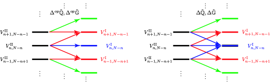
Figure 2: Action of $\Delta^{op}\tilde{\mathbb{Q}},\Delta^{op}\tilde{\mathbb{G}}$ and $\Delta\tilde{\mathbb{Q}},\Delta\tilde{\mathbb{G}}$. They map Case II states (on the left) to Case I states (on the right).

For compactness, let us define $M\equiv N-2n~{}(=N-n-n)$. By combining all the equations one is lead to the following matrix equation:

$$\begin{pmatrix}\scriptstyle{a_{4}}&\scriptstyle{a_{3}}&\scriptstyle{0}&\scriptstyle{0}\\ \scriptstyle{c_{4}}&\scriptstyle{c_{3}}&\scriptstyle{0}&\scriptstyle{0}\\ \scriptstyle{0}&\scriptstyle{0}&\scriptstyle{a_{4}}&\scriptstyle{a_{3}}\\ \scriptstyle{0}&\scriptstyle{0}&\scriptstyle{c_{4}}&\scriptstyle{c_{3}}\end{pmatrix}A~{}\mathscr{Y}^{k,l}_{n}=\begin{pmatrix}\scriptstyle{a_{2}}&\scriptstyle{a_{1}}&\scriptstyle{0}&\scriptstyle{0}\\ \scriptstyle{c_{2}}&\scriptstyle{c_{1}}&\scriptstyle{0}&\scriptstyle{0}\\ \scriptstyle{0}&\scriptstyle{0}&\scriptstyle{a_{2}}&\scriptstyle{a_{1}}\\ \scriptstyle{0}&\scriptstyle{0}&\scriptstyle{c_{2}}&\scriptstyle{c_{1}}\end{pmatrix}\left\{B^{+}\mathscr{X}^{k+1,l-1}_{n}+B^{-}\mathscr{X}^{k-1,l+1}_{n}+B\mathscr{X}^{k,l}_{n}\right\},~{}~{}$$

where the matrix on the left hand side is given by

$$A = \begin{pmatrix}\scriptstyle{N-n-\ell_{2}}&\scriptstyle{0}&\scriptstyle{\frac{\mathscr{I}_{34}}{\mathscr{Q}_{34}}}&\scriptstyle{\frac{1}{\mathscr{Q}_{43}}}\\ \scriptstyle{0}&\scriptstyle{\ell_{1}-n}&\scriptstyle{\frac{1}{\mathscr{Q}_{43}}}&\scriptstyle{\frac{\mathscr{I}_{43}}{\mathscr{Q}_{34}}}\\ \scriptstyle{(N-n-\ell_{2})(M-\delta u)}&\scriptstyle{(n-\ell_{1})\ell_{2}\mathscr{I}_{34}}&\scriptstyle{\frac{(\delta u-M+\ell_{2})\mathscr{I}_{34}}{\mathscr{Q}_{43}}}&\scriptstyle{\frac{\delta u+M+\ell_{1}-\ell_{2}\mathscr{Q}_{34}\overline{\mathscr{Q}}_{34}}{\mathscr{Q}_{43}}}\\ \scriptstyle{(N-n-\ell_{2})(\ell_{1}\mathscr{I}_{43})}&\scriptstyle{(\ell_{1}-n)(\delta u+M)}&\scriptstyle{\frac{M-\delta u-\ell_{2}+\ell_{1}\mathscr{Q}_{34}\overline{\mathscr{Q}}_{34}}{\mathscr{Q}_{43}}}&\scriptstyle{\frac{(\delta u+M+\ell_{1})\mathscr{I}_{43}}{\mathscr{Q}_{34}}}\end{pmatrix}$$ (97)

and the matrices on the right hand side by

$$B^{+}=\frac{2(\ell_{1}-k-1)\mathfrak{c}^{-}_{l-n}}{\tilde{\mathfrak{c}}^{-}_{-N}}\left(\begin{array}[]{cccc}\scriptstyle{0}&\scriptstyle{0}&\scriptstyle{0}&\scriptstyle{0}\\ \scriptstyle{0}&\scriptstyle{0}&\scriptstyle{0}&\scriptstyle{0}\\ \scriptstyle{l}&\scriptstyle{0}&\frac{\mathscr{I}_{12}}{\mathscr{Q}_{12}}&\scriptstyle{0}\\ \scriptstyle{0}&\scriptstyle{0}&\frac{1}{\mathscr{Q}_{21}}&\scriptstyle{0}\end{array}\right),\qquad B^{-}=\frac{2(\ell_{2}-l-1)\mathfrak{c}^{+}_{n-l}}{\tilde{\mathfrak{c}}^{-}_{-N}}\left(\begin{array}[]{cccc}\scriptstyle{0}&\scriptstyle{0}&\scriptstyle{0}&\scriptstyle{0}\\ \scriptstyle{0}&\scriptstyle{0}&\scriptstyle{0}&\scriptstyle{0}\\ \scriptstyle{0}&\scriptstyle{0}&\scriptstyle{0}&\frac{1}{\mathscr{Q}_{12}}\\ \scriptstyle{0}&\scriptstyle{k}&\scriptstyle{0}&\frac{\mathscr{I}_{21}}{\mathscr{Q}_{21}}\end{array}\right)$$ (106)

$$B=\begin{pmatrix}\scriptstyle{l-\ell_{2}}&\scriptstyle{0}&\scriptstyle{\frac{\mathscr{I}_{12}}{\mathscr{Q}_{12}}}&\scriptstyle{\frac{1}{\mathscr{Q}_{21}}}\\ \scriptstyle{0}&\scriptstyle{\ell_{1}-k}&\scriptstyle{\frac{1}{\mathscr{Q}_{21}}}&\scriptstyle{\frac{\mathscr{I}_{21}}{\mathscr{Q}_{12}}}\\ \scriptstyle{(l-\ell_{2})(N-\delta u)}&\scriptstyle{(\ell_{1}-k)\ell_{2}\mathscr{I}_{12}}&\scriptstyle{\frac{(N-\delta u-\ell_{2})\mathscr{I}_{12}}{\mathscr{Q}_{12}}}&\scriptstyle{\frac{N-\delta u-\ell_{1}-\ell_{2}\mathscr{Q}_{12}\overline{\mathscr{Q}}_{12}}{\mathscr{Q}_{12}}}\\ \scriptstyle{(\ell_{2}-l)(\ell_{1}\mathscr{I}_{21})}&\scriptstyle{(\ell_{1}-k)(\delta u-N)}&\scriptstyle{\frac{\delta u-N+\ell_{1}\mathscr{Q}_{12}\overline{\mathscr{Q}}_{12}+\ell_{2}}{\mathscr{Q}_{12}}}&\scriptstyle{\frac{(\delta u-N+\ell_{1})\mathscr{I}_{21}}{\mathscr{Q}_{12}}}\end{pmatrix}$$

$$\qquad-2\begin{pmatrix}\scriptstyle{0}&\scriptstyle{0}&\scriptstyle{0}&\scriptstyle{0}\\ \scriptstyle{0}&\scriptstyle{0}&\scriptstyle{0}&\scriptstyle{0}\\ \scriptstyle{\frac{l(1+n+k-\ell_{1})(l-\ell_{2})}{\tilde{\mathfrak{c}}^{-}_{-N}}}&\scriptstyle{0}&\scriptstyle{\frac{(l-\ell_{2})(1+n+k-\ell_{1})\mathscr{I}_{12}}{\tilde{\mathfrak{c}}^{-}_{-N}\mathscr{Q}_{12}}}&\scriptstyle{\frac{(\ell_{1}-k)(1+N-n+l-\ell_{2})}{\tilde{\mathfrak{c}}^{-}_{-N}\mathscr{Q}_{21}}}\\ \scriptstyle{0}&\scriptstyle{\frac{k(1+N-n+l-\ell_{2})(k-\ell_{1})}{\tilde{\mathfrak{c}}^{-}_{-N}}}&\scriptstyle{\frac{(l-\ell_{2})(1+n+k-\ell_{1})}{\tilde{\mathfrak{c}}^{-}_{-N}\mathscr{Q}_{21}}}&\scriptstyle{\frac{(\ell_{1}-k)(1+N-n+l-\ell_{2})\mathscr{I}_{21}}{\tilde{\mathfrak{c}}^{-}_{-N}\mathscr{Q}_{12}}}\end{pmatrix},$$

where we defined

$$\mathscr{Q}_{ij} = a_{i}c_{j}-a_{j}c_{i},$$

$$\overline{\mathscr{Q}}_{ij} = b_{i}d_{j}-d_{i}b_{j},$$ (107)

$$\mathscr{I}_{ij} = a_{i}d_{j}-b_{j}c_{i}.$$

These coefficients satisfy the following identity

$$\mathscr{Q}_{ij}\overline{\mathscr{Q}_{ij}}=1-\mathscr{I}_{ij}\mathscr{I}_{ji}.$$ (108)

Notice the similarities between the matrices $A,B$ and $B^{+},B^{-}$. From this, it is now straightforward to extract $\mathscr{Y}^{k,l}_{n}$ by simple linear algebra. For completeness, we will explicitly report this inverse matrix. Define

$$\mathfrak{da}\equiv\det A\frac{\mathscr{Q}_{34}^{2}}{(n-\ell_{1})(N-n-\ell_{2})} = -4\delta u^{2}+(\ell_{1}-\ell_{2})^{2}+4\ell_{1}\ell_{2}\mathscr{I}_{34}\mathscr{I}_{43}$$ (109)

$$= -4\mathfrak{c}^{+}_{1}\mathfrak{c}^{-}_{1}+4\ell_{1}\ell_{2}\mathscr{I}_{34}\mathscr{I}_{43},$$

then

$$A^{-1}=\frac{2}{\mathfrak{da}}\begin{pmatrix}\scriptstyle{\frac{1}{N-n-\ell_{2}}}&\scriptstyle{0}&\scriptstyle{0}&\scriptstyle{0}\\ \scriptstyle{0}&\scriptstyle{\frac{1}{n-\ell_{1}}}&\scriptstyle{0}&\scriptstyle{0}\\ \scriptstyle{0}&\scriptstyle{0}&\scriptstyle{\mathscr{Q}_{43}}&\scriptstyle{0}\\ \scriptstyle{0}&\scriptstyle{0}&\scriptstyle{0}&\scriptstyle{\mathscr{Q}_{43}}\end{pmatrix}\times$$ (110)

$$\times\begin{pmatrix}\scriptstyle{\frac{\mathfrak{da}}{4}-\left[M+\frac{\ell_{1}-\ell_{2}}{2}\right]\left[\mathfrak{c}^{-}_{1}+\ell_{1}\mathscr{I}_{34}\mathscr{I}_{43}\right]}&\scriptstyle{\mathscr{I}_{34}\left(\frac{\mathfrak{da}}{4}-\left[M+\frac{\ell_{1}-\ell_{2}}{2}\right]\tilde{\mathfrak{c}}^{+}_{1}\right)}&\scriptstyle{\mathfrak{c}^{-}_{1}+\ell_{1}\mathscr{I}_{34}\mathscr{I}_{43}}&\scriptstyle{\tilde{\mathfrak{c}}^{+}_{1}\mathscr{I}_{34}}\\ \scriptstyle{-\mathscr{I}_{43}\left(\frac{\mathfrak{da}}{4}+\left[M+\frac{\ell_{1}-\ell_{2}}{2}\right]\tilde{\mathfrak{c}}^{+}_{1}\right)}&\scriptstyle{-\left[M+\frac{\ell_{1}-\ell_{2}}{2}\right]\left[\mathfrak{c}^{+}_{1}+\ell_{2}\mathscr{I}_{34}\mathscr{I}_{43}\right]-\frac{\mathfrak{da}}{4}}&\scriptstyle{\tilde{\mathfrak{c}}^{+}_{1}\mathscr{I}_{43}}&\scriptstyle{\mathfrak{c}^{+}_{1}+\ell_{2}\mathscr{I}_{34}\mathscr{I}_{43}}\\ \scriptstyle{-\ell_{1}\left[M+\frac{\ell_{1}-\ell_{2}}{2}\right]\mathscr{I}_{43}}&\scriptstyle{\frac{\mathfrak{da}}{4}-\mathfrak{c}^{+}_{1}\left[M+\frac{\ell_{1}-\ell_{2}}{2}\right]}&\scriptstyle{\ell_{1}\mathscr{I}_{43}}&\scriptstyle{\mathfrak{c}^{+}_{1}}\\ \scriptstyle{\frac{\mathfrak{da}}{4}+\mathfrak{c}^{-}_{1}\left[M+\frac{\ell_{1}-\ell_{2}}{2}\right]}&\scriptstyle{\ell_{2}\left[M+\frac{\ell_{1}-\ell_{2}}{2}\right]\mathscr{I}_{34}}&\scriptstyle{-\mathfrak{c}^{-}_{1}}&\scriptstyle{-\ell_{2}\mathscr{I}_{34}}\end{pmatrix}$$

and

$$\mathscr{Y}^{k,l}_{n}=A^{-1}\begin{pmatrix}\scriptstyle{\frac{\mathscr{Q}_{32}}{\mathscr{Q}_{34}}}&\scriptstyle{\frac{\mathscr{Q}_{31}}{\mathscr{Q}_{34}}}&\scriptstyle{0}&\scriptstyle{0}\\ \scriptstyle{\frac{\mathscr{Q}_{42}}{\mathscr{Q}_{43}}}&\scriptstyle{\frac{\mathscr{Q}_{41}}{\mathscr{Q}_{43}}}&\scriptstyle{0}&\scriptstyle{0}\\ \scriptstyle{0}&\scriptstyle{0}&\scriptstyle{\frac{\mathscr{Q}_{32}}{\mathscr{Q}_{34}}}&\scriptstyle{\frac{\mathscr{Q}_{31}}{\mathscr{Q}_{34}}}\\ \scriptstyle{0}&\scriptstyle{0}&\scriptstyle{\frac{\mathscr{Q}_{42}}{\mathscr{Q}_{43}}}&\scriptstyle{\frac{\mathscr{Q}_{41}}{\mathscr{Q}_{43}}}\end{pmatrix}\left\{\mathscr{X}^{k+1,l-1}_{n}B^{+}+\mathscr{X}^{k-1,l+1}_{n}B^{-}+\mathscr{X}^{k,l}_{n}B\right\}.$$ (111)

Note that the final result for $\mathscr{Y}^{k,l}_{n}$ purely depends on the spectral parameters through their difference $\delta u$, and the representation parameters only appear in the combinations $\mathscr{Q}_{ij},\mathcal{H}_{ij}$ (modulo perhaps an overall factor), the rest being taken care of by combinatorial factors involving the integer bound-state components.

6 Complete Solution of Case III

We will perform here a similar construction as done in the previous section, in order to solve Case III in terms of Case II. Let us first set few additional notations. We introduce the S-matrix at this level in the following way:

$$\mathbb{S}|k,l\rangle^{\rm{III}}_{i}\equiv\sum_{m=0}^{k+l}\sum_{j=1}^{6}\mathscr{Z}^{k,l;j}_{m;i}|m,k+l-m\rangle^{\rm{III}}_{j}.$$ (112)

It is clear that one can repeat a very similar derivation as performed in (89) and (90), where, instead of $\mathscr{X}$, one has to think of having $\mathscr{Y}$ (and indices running over the appropriate domains). This time, moreover, one considers the action of $\Delta\mathbb{Q}^{1}_{3},\Delta\mathbb{G}_{2}^{4}$. The result is now the following matrix equations:

$$\begin{pmatrix}\scriptstyle{(n-\ell_{1})a_{3}}&\scriptstyle{0}&\scriptstyle{b_{3}}&\scriptstyle{0}&\scriptstyle{b_{4}}&\scriptstyle{0}\\ \scriptstyle{(N-n-\ell_{2})a_{4}}&\scriptstyle{b_{4}}&\scriptstyle{0}&\scriptstyle{0}&\scriptstyle{0}&\scriptstyle{-b_{3}}\\ \scriptstyle{0}&\scriptstyle{(n-\ell_{1})a_{3}}&\scriptstyle{0}&\scriptstyle{b_{3}}&\scriptstyle{(N-n-\ell_{2})a_{4}}&\scriptstyle{0}\\ \scriptstyle{0}&\scriptstyle{0}&\scriptstyle{(N-n-\ell_{2})a_{4}}&\scriptstyle{b_{4}}&\scriptstyle{0}&\scriptstyle{(n-\ell_{1})a_{3}}\end{pmatrix}\mathscr{Z}^{k,l}_{n}=$$ (113)

$$\qquad\mathscr{Y}^{k,l}_{n}\begin{pmatrix}\scriptstyle{(k-\ell_{1})a_{1}}&\scriptstyle{0}&\scriptstyle{b_{1}}&\scriptstyle{0}&\scriptstyle{b_{2}}&\scriptstyle{0}\\ \scriptstyle{(l-\ell_{2})a_{2}}&\scriptstyle{b_{2}}&\scriptstyle{0}&\scriptstyle{0}&\scriptstyle{0}&\scriptstyle{-b_{1}}\\ \scriptstyle{0}&\scriptstyle{(k-\ell_{1})a_{1}}&\scriptstyle{0}&\scriptstyle{b_{1}}&\scriptstyle{(l-\ell_{2})a_{2}}&\scriptstyle{0}\\ \scriptstyle{0}&\scriptstyle{0}&\scriptstyle{(l-\ell_{2})a_{2}}&\scriptstyle{b_{2}}&\scriptstyle{0}&\scriptstyle{(k-\ell_{1})a_{1}}\end{pmatrix},$$ (114)

and

$$\begin{pmatrix}\scriptstyle{(n-\ell_{1})c_{3}}&\scriptstyle{0}&\scriptstyle{d_{3}}&\scriptstyle{0}&\scriptstyle{d_{4}}&\scriptstyle{0}\\ \scriptstyle{(N-n-\ell_{2})c_{4}}&\scriptstyle{d_{4}}&\scriptstyle{0}&\scriptstyle{0}&\scriptstyle{0}&\scriptstyle{-d_{3}}\\ \scriptstyle{0}&\scriptstyle{(n-\ell_{1})c_{3}}&\scriptstyle{0}&\scriptstyle{d_{3}}&\scriptstyle{(N-n-\ell_{2})d_{4}}&\scriptstyle{0}\\ \scriptstyle{0}&\scriptstyle{0}&\scriptstyle{(N-n-\ell_{2})c_{4}}&\scriptstyle{d_{4}}&\scriptstyle{0}&\scriptstyle{(n-\ell_{1})c_{3}}\end{pmatrix}\mathscr{Z}^{k,l}_{n}=$$ (115)

$$\qquad\qquad\qquad\qquad\qquad\mathcal{Y}^{k,l}_{n}\begin{pmatrix}\scriptstyle{(k-\ell_{1})c_{1}}&\scriptstyle{0}&\scriptstyle{d_{1}}&\scriptstyle{0}&\scriptstyle{d_{2}}&\scriptstyle{0}\\ \scriptstyle{(l-\ell_{2})c_{2}}&\scriptstyle{d_{2}}&\scriptstyle{0}&\scriptstyle{0}&\scriptstyle{0}&\scriptstyle{-d_{1}}\\ \scriptstyle{0}&\scriptstyle{(k-\ell_{1})c_{1}}&\scriptstyle{0}&\scriptstyle{d_{1}}&\scriptstyle{(l-\ell_{2})c_{2}}&\scriptstyle{0}\\ \scriptstyle{0}&\scriptstyle{0}&\scriptstyle{(l-\ell_{2})c_{2}}&\scriptstyle{d_{2}}&\scriptstyle{0}&\scriptstyle{(k-\ell_{1})c_{1}}\end{pmatrix},$$

where

$$\mathscr{Z}^{k,l}_{n} \equiv \begin{pmatrix}\scriptstyle{\mathscr{Z}^{k,l;1}_{n;1}}&\scriptstyle{\mathscr{Z}^{k,l;1}_{n;2}}&\scriptstyle{\mathscr{Z}^{k,l;1}_{n;3}}&\scriptstyle{\mathscr{Z}^{k,l;1}_{n;4}}&\scriptstyle{\mathscr{Z}^{k,l;1}_{n;5}}&\scriptstyle{\mathscr{Z}^{k,l;1}_{n;6}}\\ \scriptstyle{\mathscr{Z}^{k,l;2}_{n;1}}&\scriptstyle{\mathscr{Z}^{k,l;2}_{n;2}}&\scriptstyle{\mathscr{Z}^{k,l;2}_{n;3}}&\scriptstyle{\mathscr{Z}^{k,l;2}_{n;4}}&\scriptstyle{\mathscr{Z}^{k,l;2}_{n;5}}&\scriptstyle{\mathscr{Z}^{k,l;2}_{n;6}}\\ \scriptstyle{\mathscr{Z}^{k,l;3}_{n;1}}&\scriptstyle{\mathscr{Z}^{k,l;3}_{n;2}}&\scriptstyle{\mathscr{Z}^{k,l;3}_{n;3}}&\scriptstyle{\mathscr{Z}^{k,l;3}_{n;4}}&\scriptstyle{\mathscr{Z}^{k,l;3}_{n;5}}&\scriptstyle{\mathscr{Z}^{k,l;3}_{n;6}}\\ \scriptstyle{\mathscr{Z}^{k,l;4}_{n;1}}&\scriptstyle{\mathscr{Z}^{k,l;4}_{n;2}}&\scriptstyle{\mathscr{Z}^{k,l;4}_{n;3}}&\scriptstyle{\mathscr{Z}^{k,l;4}_{n;4}}&\scriptstyle{\mathscr{Z}^{k,l;4}_{n;5}}&\scriptstyle{\mathscr{Z}^{k,l;4}_{n;6}}\\ \scriptstyle{\mathscr{Z}^{k,l;5}_{n;1}}&\scriptstyle{\mathscr{Z}^{k,l;5}_{n;2}}&\scriptstyle{\mathscr{Z}^{k,l;5}_{n;3}}&\scriptstyle{\mathscr{Z}^{k,l;5}_{n;4}}&\scriptstyle{\mathscr{Z}^{k,l;5}_{n;5}}&\scriptstyle{\mathscr{Z}^{k,l;5}_{n;6}}\\ \scriptstyle{\mathscr{Z}^{k,l;6}_{n;1}}&\scriptstyle{\mathscr{Z}^{k,l;6}_{n;2}}&\scriptstyle{\mathscr{Z}^{k,l;6}_{n;3}}&\scriptstyle{\mathscr{Z}^{k,l;6}_{n;4}}&\scriptstyle{\mathscr{Z}^{k,l;6}_{n;5}}&\scriptstyle{\mathscr{Z}^{k,l;6}_{n;6}}\end{pmatrix}.$$ (116)

Again the relation with (3) is apparent.

However, it is readily checked that these equations are not independent. Hence, once again one needs additional equations, as in the previous section it was required in order to compute $\mathscr{Y}$. In that case, they were provided by Yangian generators. In this case we are more fortunate and do not need the Yangian, since one can consider the action of $\Delta\mathbb{Q}^{2}_{4}$ and $\Delta\mathbb{G}^{3}_{1}$. It is easy to check that, by repeating the above procedure using these additional symmetries, one arrives this time at the following matrix equations:

$$\begin{pmatrix}\scriptstyle{na_{3}}&\scriptstyle{0}&\scriptstyle{b_{3}}&\scriptstyle{0}&\scriptstyle{0}&\scriptstyle{-b_{4}}\\ \scriptstyle{(N-n)a_{4}}&\scriptstyle{b_{4}}&\scriptstyle{0}&\scriptstyle{0}&\scriptstyle{b_{3}}&\scriptstyle{0}\\ \scriptstyle{0}&\scriptstyle{na_{3}}&\scriptstyle{0}&\scriptstyle{b_{3}}&\scriptstyle{0}&\scriptstyle{(N-n)a_{4}}\\ \scriptstyle{0}&\scriptstyle{0}&\scriptstyle{(N-n)a_{4}}&\scriptstyle{b_{4}}&\scriptstyle{-na_{3}}&\scriptstyle{0}\end{pmatrix}\mathscr{Z}^{k,l}_{n}=\tilde{\mathscr{Y}}^{k,l}_{n}\begin{pmatrix}\scriptstyle{ka_{1}}&\scriptstyle{0}&\scriptstyle{b_{1}}&\scriptstyle{0}&\scriptstyle{0}&\scriptstyle{-b_{2}}\\ \scriptstyle{la_{2}}&\scriptstyle{b_{2}}&\scriptstyle{0}&\scriptstyle{0}&\scriptstyle{b_{1}}&\scriptstyle{0}\\ \scriptstyle{0}&\scriptstyle{ka_{1}}&\scriptstyle{0}&\scriptstyle{b_{1}}&\scriptstyle{0}&\scriptstyle{la_{2}}\\ \scriptstyle{0}&\scriptstyle{0}&\scriptstyle{la_{2}}&\scriptstyle{b_{2}}&\scriptstyle{-ka_{1}}&\scriptstyle{0}\end{pmatrix}$$ (117)

and

$$\begin{pmatrix}\scriptstyle{nc_{3}}&\scriptstyle{0}&\scriptstyle{d_{3}}&\scriptstyle{0}&\scriptstyle{0}&\scriptstyle{-d_{4}}\\ \scriptstyle{(N-n)c_{4}}&\scriptstyle{d_{4}}&\scriptstyle{0}&\scriptstyle{0}&\scriptstyle{d_{3}}&\scriptstyle{0}\\ \scriptstyle{0}&\scriptstyle{nc_{3}}&\scriptstyle{0}&\scriptstyle{d_{3}}&\scriptstyle{0}&\scriptstyle{(N-n)c_{4}}\\ \scriptstyle{0}&\scriptstyle{0}&\scriptstyle{(N-n)c_{4}}&\scriptstyle{d_{4}}&\scriptstyle{-nc_{3}}&\scriptstyle{0}\end{pmatrix}\mathscr{Z}^{k,l}_{n}=\tilde{\mathscr{Y}}^{k,l}_{n}\begin{pmatrix}\scriptstyle{kc_{1}}&\scriptstyle{0}&\scriptstyle{d_{1}}&\scriptstyle{0}&\scriptstyle{0}&\scriptstyle{-d_{2}}\\ \scriptstyle{lc_{2}}&\scriptstyle{d_{2}}&\scriptstyle{0}&\scriptstyle{0}&\scriptstyle{d_{1}}&\scriptstyle{0}\\ \scriptstyle{0}&\scriptstyle{kc_{1}}&\scriptstyle{0}&\scriptstyle{d_{1}}&\scriptstyle{0}&\scriptstyle{lc_{2}}\\ \scriptstyle{0}&\scriptstyle{0}&\scriptstyle{lc_{2}}&\scriptstyle{d_{2}}&\scriptstyle{-kc_{1}}&\scriptstyle{0}\end{pmatrix},$$ (118)

where we have defined

$$\tilde{\mathscr{Y}}^{k,l}_{n} \equiv \begin{pmatrix}\mathscr{Y}^{k-1,l;1}_{n-1;1}&\mathscr{Y}^{k,l-1;1}_{n-1;2}&\mathscr{Y}^{k-1,l;1}_{n-1;3}&\mathscr{Y}^{k,l-1;1}_{n-1;4}\\ \mathscr{Y}^{k-1,l;2}_{n;1}&\mathscr{Y}^{k,l-1;2}_{n;2}&\mathscr{Y}^{k-1,l;2}_{n;3}&\mathscr{Y}^{k,l-1;2}_{n;4}\\ \mathscr{Y}^{k-1,l;3}_{n-1;1}&\mathscr{Y}^{k,l-1;3}_{n-1;2}&\mathscr{Y}^{k-1,l;3}_{n-1;3}&\mathscr{Y}^{k,l-1;3}_{n-1;4}\\ \mathscr{Y}^{k-1,l;4}_{n;1}&\mathscr{Y}^{k,l-1;4}_{n;2}&\mathscr{Y}^{k-1,l;4}_{n;3}&\mathscr{Y}^{k,l-1;4}_{n;4}\end{pmatrix}.$$ (119)

Combining all of the above equations is sufficient in order to solve for $\mathscr{Z}$. To be more precise, one can write the equation for $\mathscr{Z}^{k,l}_{n}$ in the following way:

$$\left(\begin{array}[]{cccccc}\scriptstyle{(n-\ell_{1})\mathscr{Q}_{43}}&\scriptstyle{0}&\scriptstyle{\mathscr{I}_{43}}&\scriptstyle{0}&\scriptstyle{1}&\scriptstyle{0}\\ \scriptstyle{0}&\scriptstyle{1}&\scriptstyle{0}&\scriptstyle{0}&\scriptstyle{0}&\scriptstyle{-\mathscr{I}_{43}}\\ \scriptstyle{0}&\scriptstyle{(n-\ell_{1})\mathscr{Q}_{43}}&\scriptstyle{0}&\scriptstyle{\mathscr{I}_{43}}&\scriptstyle{0}&\scriptstyle{0}\\ \scriptstyle{-n\mathscr{Q}_{43}}&\scriptstyle{0}&\scriptstyle{-\mathscr{I}_{43}}&\scriptstyle{0}&\scriptstyle{0}&\scriptstyle{1}\\ \scriptstyle{0}&\scriptstyle{-1}&\scriptstyle{0}&\scriptstyle{0}&\scriptstyle{-\mathscr{I}_{43}}&\scriptstyle{0}\\ \scriptstyle{0}&\scriptstyle{-n\mathscr{Q}_{43}}&\scriptstyle{0}&\scriptstyle{-\mathscr{I}_{43}}&\scriptstyle{0}&\scriptstyle{0}\end{array}\right)\mathscr{Z}^{k,l}_{n}=$$ (126)

$$\qquad\qquad\qquad\check{\mathscr{S}}^{k,l}_{n}\left(\begin{array}[]{cccccc}\scriptstyle{(\ell_{1}-k)\mathscr{Q}_{14}}&\scriptstyle{0}&\scriptstyle{\mathscr{I}_{41}}&\scriptstyle{0}&\scriptstyle{\mathscr{I}_{42}}&\scriptstyle{0}\\ \scriptstyle{(l-\ell_{2})\mathscr{Q}_{42}}&\scriptstyle{\mathscr{I}_{42}}&\scriptstyle{0}&\scriptstyle{0}&\scriptstyle{0}&\scriptstyle{-\mathscr{I}_{41}}\\ \scriptstyle{0}&\scriptstyle{(\ell_{1}-k)\mathscr{Q}_{14}}&\scriptstyle{0}&\scriptstyle{\mathscr{I}_{41}}&\scriptstyle{(\ell_{2}-l)\mathscr{Q}_{42}}&\scriptstyle{0}\\ \scriptstyle{0}&\scriptstyle{0}&\scriptstyle{(l-\ell_{2})\mathscr{Q}_{42}}&\scriptstyle{\mathscr{I}_{42}}&\scriptstyle{0}&\scriptstyle{(\ell_{1}-k)\mathscr{Q}_{14}}\\ \scriptstyle{k\mathscr{Q}_{14}}&\scriptstyle{0}&\scriptstyle{-\mathscr{I}_{41}}&\scriptstyle{0}&\scriptstyle{0}&\scriptstyle{\mathscr{I}_{42}}\\ \scriptstyle{-l\mathscr{Q}_{42}}&\scriptstyle{-\mathscr{I}_{42}}&\scriptstyle{0}&\scriptstyle{0}&\scriptstyle{-\mathscr{I}_{41}}&\scriptstyle{0}\\ \scriptstyle{0}&\scriptstyle{k\mathscr{Q}_{14}}&\scriptstyle{0}&\scriptstyle{-\mathscr{I}_{41}}&\scriptstyle{0}&\scriptstyle{-l\mathscr{Q}_{42}}\\ \scriptstyle{0}&\scriptstyle{0}&\scriptstyle{-l\mathscr{Q}_{42}}&\scriptstyle{-\mathscr{I}_{42}}&\scriptstyle{-k\mathscr{Q}_{14}}&\scriptstyle{0}\end{array}\right),$$ (135)

with

$$\check{\mathscr{Y}}^{k,l}_{n}\equiv\left(\begin{array}[]{cccccccccccc}\scriptstyle{\mathscr{Y}^{k,l;1}_{n;1}}&\scriptstyle{\mathscr{Y}^{k,l;1}_{n;2}}&\scriptstyle{\mathscr{Y}^{k,l;1}_{n;3}}&\scriptstyle{\mathscr{Y}^{k,l;1}_{n;4}}&\scriptstyle{0}&\scriptstyle{0}&\scriptstyle{0}&\scriptstyle{0}\\ \scriptstyle{\mathscr{Y}^{k,l;2}_{n;1}}&\scriptstyle{\mathscr{Y}^{k,l;2}_{n;2}}&\scriptstyle{\mathscr{Y}^{k,l;2}_{n;3}}&\scriptstyle{\mathscr{Y}^{k,l;2}_{n;4}}&\scriptstyle{0}&\scriptstyle{0}&\scriptstyle{0}&\scriptstyle{0}\\ \scriptstyle{\mathscr{Y}^{k,l;3}_{n;1}}&\scriptstyle{\mathscr{Y}^{k,l;3}_{n;2}}&\scriptstyle{\mathscr{Y}^{k,l;3}_{n;3}}&\scriptstyle{\mathscr{Y}^{k,l;3}_{n;4}}&\scriptstyle{0}&\scriptstyle{0}&\scriptstyle{0}&\scriptstyle{0}\\ \scriptstyle{0}&\scriptstyle{0}&\scriptstyle{0}&\scriptstyle{0}&\scriptstyle{\mathscr{Y}^{k-1,l;1}_{n-1;1}}&\scriptstyle{\mathscr{Y}^{k,l-1;1}_{n-1;2}}&\scriptstyle{\mathscr{Y}^{k-1,l;1}_{n-1;3}}&\scriptstyle{\mathscr{Y}^{k,l-1;1}_{n-1;4}}\\ \scriptstyle{0}&\scriptstyle{0}&\scriptstyle{0}&\scriptstyle{0}&\scriptstyle{\mathscr{Y}^{k-1,l;2}_{n;1}}&\scriptstyle{\mathscr{Y}^{k,l-1;2}_{n;2}}&\scriptstyle{\mathscr{Y}^{k-1,l;2}_{n;3}}&\scriptstyle{\mathscr{Y}^{k,l-1;2}_{n;4}}\\ \scriptstyle{0}&\scriptstyle{0}&\scriptstyle{0}&\scriptstyle{0}&\scriptstyle{\mathscr{Y}^{k-1,l;3}_{n-1;1}}&\scriptstyle{\mathscr{Y}^{k,l-1;3}_{n-1;2}}&\scriptstyle{\mathscr{Y}^{k-1,l;3}_{n-1;3}}&\scriptstyle{\mathscr{Y}^{k,l-1;3}_{n-1;4}}\end{array}\right).$$ (142)

The explicit matrix inversion gives

$$\mathscr{Z}=\left(\begin{array}[]{llllll}\frac{1}{\ell_{1}\mathscr{Q}_{34}}&\frac{1}{\ell_{1}\mathscr{Q}_{34}\mathscr{I}_{43}}&\scriptstyle{0}&\frac{1}{\ell_{1}\mathscr{Q}_{34}}&\frac{1}{\ell_{1}\mathscr{Q}_{34}\mathscr{I}_{43}}&\scriptstyle{0}\\ \scriptstyle{0}&\scriptstyle{0}&\frac{1}{\ell_{1}\mathscr{Q}_{34}}&\scriptstyle{0}&\scriptstyle{0}&\frac{1}{\ell_{1}\mathscr{Q}_{34}}\\ \frac{n}{\ell_{1}\mathscr{I}_{43}}&\frac{n-\ell_{1}}{\ell_{1}\mathscr{I}_{43}^{2}}&\frac{1}{\ell_{1}\mathscr{Q}_{34}\mathscr{I}_{43}^{2}}&\frac{n-\ell_{1}}{\ell_{1}\mathscr{I}_{43}}&\frac{n}{\ell_{1}\mathscr{I}_{43}^{2}}&\frac{1}{\ell_{1}\mathscr{Q}_{34}\mathscr{I}_{43}^{2}}\\ \scriptstyle{0}&\scriptstyle{0}&\frac{n}{\ell_{1}\mathscr{I}_{43}}&\scriptstyle{0}&\scriptstyle{0}&\frac{n-\ell_{1}}{\ell_{1}\mathscr{I}_{43}}\\ \scriptstyle{0}&\scriptstyle{0}&\frac{1}{\ell_{1}\mathscr{Q}_{43}\mathscr{I}_{43}}&\scriptstyle{0}&\scriptstyle{-}\frac{1}{\mathscr{I}_{43}}&\frac{1}{\ell_{1}\mathscr{Q}_{43}\mathscr{I}_{43}}\\ \scriptstyle{0}&\scriptstyle{-}\frac{1}{\mathscr{I}_{43}}&\frac{1}{\ell_{1}\mathscr{Q}_{34}\mathscr{I}_{43}}&\scriptstyle{0}&\scriptstyle{0}&\frac{1}{\ell_{1}\mathscr{Q}_{34}\mathscr{I}_{43}}\end{array}\right)\check{\mathscr{Y}}^{k,l}_{n}\times$$ (149)

$$\qquad\qquad\qquad\qquad\times\left(\begin{array}[]{cccccc}\scriptstyle{(\ell_{1}-k)\mathscr{Q}_{14}}&\scriptstyle{0}&\scriptstyle{\mathscr{I}_{41}}&\scriptstyle{0}&\scriptstyle{\mathscr{I}_{42}}&\scriptstyle{0}\\ \scriptstyle{(l-\ell_{2})\mathscr{Q}_{42}}&\scriptstyle{\mathscr{I}_{42}}&\scriptstyle{0}&\scriptstyle{0}&\scriptstyle{0}&\scriptstyle{-\mathscr{I}_{41}}\\ \scriptstyle{0}&\scriptstyle{(\ell_{1}-k)\mathscr{Q}_{14}}&\scriptstyle{0}&\scriptstyle{\mathscr{I}_{41}}&\scriptstyle{(\ell_{2}-l)\mathscr{Q}_{42}}&\scriptstyle{0}\\ \scriptstyle{0}&\scriptstyle{0}&\scriptstyle{(l-\ell_{2})\mathscr{Q}_{42}}&\scriptstyle{\mathscr{I}_{42}}&\scriptstyle{0}&\scriptstyle{(\ell_{1}-k)\mathscr{Q}_{14}}\\ \scriptstyle{k\mathscr{Q}_{14}}&\scriptstyle{0}&\scriptstyle{-\mathscr{I}_{41}}&\scriptstyle{0}&\scriptstyle{0}&\scriptstyle{\mathscr{I}_{42}}\\ \scriptstyle{-l\mathscr{Q}_{42}}&\scriptstyle{-\mathscr{I}_{42}}&\scriptstyle{0}&\scriptstyle{0}&\scriptstyle{-\mathscr{I}_{41}}&\scriptstyle{0}\\ \scriptstyle{0}&\scriptstyle{k\mathscr{Q}_{14}}&\scriptstyle{0}&\scriptstyle{-\mathscr{I}_{41}}&\scriptstyle{0}&\scriptstyle{-l\mathscr{Q}_{42}}\\ \scriptstyle{0}&\scriptstyle{0}&\scriptstyle{-l\mathscr{Q}_{42}}&\scriptstyle{-\mathscr{I}_{42}}&\scriptstyle{-k\mathscr{Q}_{14}}&\scriptstyle{0}\end{array}\right).$$ (158)

It is now straightforward to do the matrix multiplication. This solves the final case. Once again, the dependence of the entries solely on the difference of the spectral parameters, and on the characteristic combinations of representation labels already observed in Case II, is a noticeable feature of the result.

7 Reduction and Comparison

Let us now compare our formulae with the known S-matrices. Here, one runs into potential difficulties. The formulae from the previous sections were derived for generic bound states, and one might wonder whether there could be obstructions for small bound states. A first problem arises when $n$ is comparable to $\ell_{1},\ell_{2}$. A second problem is encountered for $n=0,n=k+l$, since the basis of two-particle states in these two cases is lower-dimensional. One can wonder whether our formulae

$${\mathbb{S}}|k,l\rangle^{\rm{I}} = \sum_{n=0}^{k+l}\mathscr{X}^{k,l}_{n}|n,N-n\rangle^{\rm{I}}$$ (159)

$${\mathbb{S}}|k,l\rangle^{\rm{II}}_{i} = \sum_{n=0}^{k+l}\sum_{j=1}^{4}\mathscr{Y}^{k,l;j}_{n;i}|n,N-n\rangle^{\rm{II}}_{j}$$ (160)

$${\mathbb{S}}|k,l\rangle^{\rm{III}}_{i} = \sum_{n=0}^{k+l}\sum_{j=1}^{6}\mathscr{Z}^{k,l;j}_{n;i}|n,N-n\rangle^{\rm{III}}_{j},$$ (161)

with $N=k+l$ and $\mathscr{Y},\mathscr{Z}$ given by (111) and (149), remain valid also for these particular values.

It turns out that this is indeed the case. Let us deal with the first problem. One can see from (4.1) that, when $n>\ell_{1}$, precisely the unwanted S-matrix elements vanish, basically thanks to the vanishing of the correspondent coefficients $\mathscr{X}^{k,l}_{n}$.

Concerning the second potential problem, we notice that the issue arises only for Case II and III states. In Case II, the corresponding sum on the right hand side of (160) contains terms like

$$\mathscr{Y}^{k,l;4}_{0;i}|0,N\rangle^{\rm{II}}_{4}.$$ (162)

But, as seen from (2), $|0,N\rangle^{\rm{II}}_{4}$ is not well-defined (actually it is not part of our bound state representation). Hence, the S-matrix transition amplitudes toward these states, $\mathscr{Y}^{k,l;4}_{0;i}$, should vanish identically. We verified that this indeed turns out to be the case, which means that these states completely decouple.

More specifically, from (4.1) it can be shown that

$$\mathscr{X}^{k+1,l-1}_{0} = \frac{\ell_{2}-l}{\delta u-\frac{\ell_{1}-\ell_{2}}{2}-l+1}\mathscr{X}^{k,l}_{0}$$ (163)

$$\mathscr{X}^{k-1,l+1}_{0} = \frac{\delta u-\frac{\ell_{1}-\ell_{2}}{2}-l}{\ell_{2}-l-1}\mathscr{X}^{k,l}_{0}.$$ (164)

This means that in (111) one can pull out a factor $\mathscr{X}^{k,l}_{0}$. The remaining matrix part is straightforwardly seen to have zeroes for the states corresponding to the amplitudes $\mathscr{Y}^{k,l;4}_{0;i}$, for all $i=1,2,3,4$ as indeed should be the case. In other words, one can unambiguously write

$${\mathbb{S}}|k,l\rangle^{\rm{II}}_{i}=\sum_{n=0}^{k+l}\sum_{j=1}^{4}\mathscr{Y}^{k,l;j}_{n;i}|n,N-n\rangle^{\rm{II}}_{j},$$ (165)

where $\mathscr{Y}^{k,l;j}_{n;i}$ is given by the complete $4\times 4$ matrix from (111). The same should be true for Case III states.

One can now compare our coefficients against the known S-matrices. Complete agreement is found with ${\mathbb{S}}^{AA},{\mathbb{S}}^{AB},{\mathbb{S}}^{BB}$ from [6, 15, 43]. We also checked several coefficients of the S-matrix ${\mathbb{S}}^{1\ell}$ from [31] which also agree with our findings.

Appendix A Yangians and Coproducts

The double Yangian $DY(\mathfrak{g})$ of a (simple) Lie algebra $\mathfrak{g}$ is a deformation of the universal enveloping algebra $U(\mathfrak{g}[u,u^{-1}])$ of the loop algebra $\mathfrak{g}[u,u^{-1}]$. The Yangian is generated by level $n$ generators $\mathbb{J}^{A}_{n},\ n\in\mathbb{Z}$ that satisfy the commutation relations

$$\ [\mathbb{J}^{A}_{m},\mathbb{J}^{B}_{n}]=F^{AB}_{C}\mathbb{J}^{C}_{m+n}+\mathcal{O}(\hbar),$$ (166)

where $F^{AB}_{C}$ are the structure constants of $\mathfrak{g}$. The level-0 generators $\mathbb{J}_{0}^{A}$ span the Lie-algebra. The $\mathfrak{su}(2|2)$ Yangian has the following coproduct [45, 46, 44]:

$$\Delta(\mathbb{J}^{A}_{n}) = \mathbb{J}^{A}_{n}\otimes\mathbbm{1}+\mathcal{U}^{[A]}\otimes\mathbb{J}^{A}_{n}+\frac{\hbar}{2}\sum_{m=0}^{n-1}F_{BC}^{A}\mathbb{J}^{B}_{n-1-m}\mathcal{U}^{[C]}\otimes\mathbb{J}^{C}_{m}+\mathcal{O}(\hbar^{2}),$$

$$\Delta(\mathcal{U}) = \mathcal{U}\otimes\mathcal{U},$$ (167)

where $\mathcal{U}$, the ‘braiding factor’, equals $e^{i\frac{p}{2}}$, and $\hbar=1/g$.

An important representation of the Yangian is the evaluation representation. This representation consists of states $|u\rangle$, with action $\mathbb{J}^{A}_{n}|u\rangle=u^{n}\mathbb{J}^{A}_{0}|u\rangle$. In this representation the coproduct structure is fixed in terms of the coproducts of $\mathbb{J}_{0},\mathbb{J}_{1}$. For the remainder of this paper we will work in this representation, and identify $\mathbb{J}_{1}\equiv\hat{\mathbb{J}}=u\mathbb{J}$ for the $\mathfrak{su}(2|2)$ Yangian. The spectral parameter $u$ depends on $x^{\pm}$, as one can see from formula (36).

The S-matrix is a map between the following representations:

$${\mathbb{S}}:~{}~{}{\mathscr{V}}_{\ell_{1}}(p_{1},e^{ip_{2}})\otimes{\mathscr{V}}_{\ell_{2}}(p_{2},1)\longrightarrow{\mathscr{V}}_{\ell_{1}}(p_{1},1)\otimes{\mathscr{V}}_{\ell_{2}}(p_{2},e^{ip_{1}}),$$ (168)

where ${\mathscr{V}}_{\ell_{i}}(p_{i},e^{2i\xi})$ is the $\ell_{i}$-bound state representation with parameters $a_{i},b_{i},c_{i},d_{i}$ with the choice of $\zeta=e^{2i\xi}$. This specific choice removes the braiding factor $\mathcal{U}$ from appearing explicitly in the formulas [15].

The bound state S-matrices are now fixed, up to an overall phase, by requiring invariance under the coproducts of the (Yangian) symmetry generators

$${\mathbb{S}}~{}\Delta(\mathbb{J}^{A}) = \Delta^{op}(\mathbb{J}^{A})~{}{\mathbb{S}},$$

$${\mathbb{S}}~{}\Delta(\hat{\mathbb{J}}^{A}) = \Delta^{op}(\hat{\mathbb{J}}^{A})~{}{\mathbb{S}},$$ (169)

where $\Delta^{op}=P\Delta$, with $P$ the graded permutation.

For completeness and future reference, we give the explicit formulas for the coproducts and for the parameters $a_{i},b_{i},c_{i},d_{i}$. First, the $\mathfrak{su}(2|2)$ operators:

$$\Delta(\mathbb{J}_{0}^{A})=\mathbb{J}_{1;0}^{A}+\mathbb{J}_{2;0}^{A}.$$ (170)

The coproducts of the Yangian generators are then given by [44]

$$\Delta(\hat{\mathbb{L}}^{a}_{\ b}) = \hat{\mathbb{L}}^{\ a}_{1;b}+\hat{\mathbb{L}}^{\ a}_{2;b}+\frac{1}{2}\mathbb{L}^{\ c}_{1;b}\mathbb{L}^{\ a}_{2;c}-\frac{1}{2}\mathbb{L}^{\ a}_{1;c}\mathbb{L}^{\ c}_{2;b}-\frac{1}{2}\mathbb{G}^{\ \gamma}_{1;b}\mathbb{Q}^{\ a}_{2;\gamma}-\frac{1}{2}\mathbb{Q}^{\ a}_{1;\gamma}\mathbb{G}^{\ \gamma}_{2;b}$$

$$+\frac{1}{4}\delta^{a}_{b}\mathbb{G}^{\ \gamma}_{1;c}\mathbb{Q}^{\ c}_{2;\gamma}+\frac{1}{4}\delta^{a}_{b}\mathbb{Q}^{\ c}_{1;\gamma}\mathbb{G}^{\ \gamma}_{2;c}~{},$$

$$\Delta(\hat{\mathbb{R}}^{\alpha}_{\ \beta}) = \hat{\mathbb{R}}^{\ \alpha}_{1;\beta}+\hat{\mathbb{R}}^{\ \alpha}_{2;\beta}-\frac{1}{2}\mathbb{R}^{\ \gamma}_{1;\beta}\mathbb{R}^{\ \alpha}_{2;\gamma}+\frac{1}{2}\mathbb{R}^{\ \alpha}_{1;\gamma}\mathbb{R}^{\ \gamma}_{2;\beta}+\frac{1}{2}\mathbb{G}^{\ \alpha}_{1;c}\mathbb{Q}^{\ c}_{2;\beta}+\frac{1}{2}\mathbb{Q}^{\ c}_{1;\beta}\mathbb{G}^{\ \alpha}_{2;c}$$ (171)

$$-\frac{1}{4}\delta^{\alpha}_{\beta}\mathbb{G}^{\ \gamma}_{1;c}\mathbb{Q}^{\ c}_{2;\gamma}-\frac{1}{4}\delta^{\alpha}_{\beta}\mathbb{Q}^{\ c}_{1;\gamma}\mathbb{G}^{\ \gamma}_{2;c}~{},$$

$$\Delta(\hat{\mathbb{Q}}^{a}_{\ \beta}) = \hat{\mathbb{Q}}^{\ a}_{1;\beta}+\hat{\mathbb{Q}}^{\ a}_{2;\beta}-\frac{1}{2}\mathbb{R}^{\ \gamma}_{1;\beta}\mathbb{Q}^{\ a}_{2;\gamma}+\frac{1}{2}\mathbb{Q}^{\ a}_{1;\gamma}\mathbb{R}^{\ \gamma}_{2;\beta}-\frac{1}{2}\mathbb{L}^{\ a}_{1;c}\mathbb{Q}^{\ c}_{2;\beta}+\frac{1}{2}\mathbb{Q}^{\ c}_{1;\beta}\mathbb{L}^{\ a}_{2;c}$$

$$-\frac{1}{4}\mathbb{H}_{1}\mathbb{Q}^{\ a}_{2;\beta}+\frac{1}{4}\mathbb{Q}^{\ a}_{1;\beta}\mathbb{H}_{2}+\frac{1}{2}\epsilon_{\beta\gamma}\epsilon^{ad}\mathbb{C}_{1}\mathbb{G}^{\ \gamma}_{2;d}-\frac{1}{2}\epsilon_{\beta\gamma}\epsilon^{ad}\mathbb{G}^{\ \gamma}_{1;d}\mathbb{C}_{2}~{},$$

$$\Delta(\hat{\mathbb{G}}^{\alpha}_{\ b}) = \hat{\mathbb{G}}^{\ \alpha}_{1;b}+\hat{\mathbb{G}}^{\ \alpha}_{2;b}+\frac{1}{2}\mathbb{L}^{\ c}_{1;b}\mathbb{G}^{\ \alpha}_{2;c}-\frac{1}{2}\mathbb{G}^{\ \alpha}_{1;c}\mathbb{L}^{\ c}_{2;b}+\frac{1}{2}\mathbb{R}^{\ \alpha}_{1;\gamma}\mathbb{G}^{\ \gamma}_{2;b}-\frac{1}{2}\mathbb{G}^{\ \gamma}_{1;b}\mathbb{R}^{\ \alpha}_{2;\gamma}$$

$$+\frac{1}{4}\mathbb{H}_{1}\mathbb{G}^{\ \alpha}_{2;b}-\frac{1}{4}\mathbb{G}^{\ \alpha}_{1;b}\mathbb{H}_{2}-\frac{1}{2}\epsilon_{bc}\epsilon^{\alpha\gamma}\mathbb{C}^{{\dagger}}_{1}\mathbb{Q}^{\ c}_{2;\gamma}+\frac{1}{2}\epsilon_{bc}\epsilon^{\alpha\gamma}\mathbb{Q}^{\ c}_{1;\gamma}\mathbb{C}^{{\dagger}}_{2}~{},$$

and for the central charges

$$\Delta(\hat{\mathbb{H}}) = \hat{\mathbb{H}}_{1}+\hat{\mathbb{H}}_{2}+\mathbb{C}_{1}\mathbb{C}^{{\dagger}}_{2}-\mathbb{C}^{{\dagger}}_{1}\mathbb{C}_{2},$$

$$\Delta(\hat{\mathbb{C}}) = \hat{\mathbb{C}}_{1}+\hat{\mathbb{C}}_{2}+\frac{1}{2}\mathbb{H}_{1}\mathbb{C}_{2}-\frac{1}{2}\mathbb{C}_{1}\mathbb{H}_{2},$$ (172)

$$\Delta(\hat{\mathbb{C}}^{{\dagger}}) = \hat{\mathbb{C}}^{{\dagger}}_{1}+\hat{\mathbb{C}}^{{\dagger}}_{2}+\frac{1}{2}\mathbb{H}_{1}\mathbb{C}^{{\dagger}}_{2}-\frac{1}{2}\mathbb{C}^{{\dagger}}_{1}\mathbb{H}_{2}.$$

The product is ordered, e.g. $\mathbb{Q}_{1}\mathbb{Q}_{2}$ means first applying $\mathbb{Q}_{2}$, then $\mathbb{Q}_{1}$ (as differential operators). Finally, the coefficients used in $\Delta$ are given by:

$$\begin{array}[]{lll}a_{1}=\sqrt{\frac{g}{2\ell_{1}}}\eta_{1},&{}&b_{1}=ie^{ip_{2}}\sqrt{\frac{g}{2\ell_{1}}}~{}\frac{1}{\eta_{1}}\left(\frac{x_{1}^{+}}{x_{1}^{-}}-1\right),\\ c_{1}=-e^{-ip_{2}}\sqrt{\frac{g}{2\ell_{1}}}\frac{\eta_{1}}{x_{1}^{+}},&{}&d_{1}=i\sqrt{\frac{g}{2\ell_{1}}}\frac{x_{1}^{+}}{\eta_{1}}\left(\frac{x_{1}^{-}}{x_{1}^{+}}-1\right),\\ \eta_{1}=e^{i\frac{p_{1}}{4}}e^{i\frac{p_{2}}{2}}\sqrt{ix^{-}_{1}-ix^{+}_{1}},&{}&{}\\ {}&{}&{}\\ a_{2}=\sqrt{\frac{g}{2\ell_{2}}}\eta_{2},&{}&b_{2}=i\sqrt{\frac{g}{2\ell_{2}}}\frac{1}{\eta_{2}}\left(\frac{x_{2}^{+}}{x_{2}^{-}}-1\right),\\ c_{2}=-\sqrt{\frac{g}{2\ell_{2}}}\frac{\eta_{2}}{x_{2}^{+}},&{}&d_{2}=i\sqrt{\frac{g}{2\ell_{2}}}\frac{x_{2}^{+}}{\eta_{2}}\left(\frac{x_{2}^{-}}{x_{2}^{+}}-1\right),\\ \eta_{2}=e^{i\frac{p_{2}}{4}}\sqrt{ix^{-}_{2}-ix^{+}_{2}}.&{}&{}\end{array}$$ (180)

The coefficients in $\Delta^{op}$ are given by:

$$\begin{array}[]{lll}a_{3}=\sqrt{\frac{g}{2\ell_{1}}}\eta^{op}_{1},&{}&b_{3}=i\sqrt{\frac{g}{2\ell_{1}}}\frac{1}{\eta^{op}_{1}}\left(\frac{x_{1}^{+}}{x_{1}^{-}}-1\right),\\ c_{3}=-\sqrt{\frac{g}{2\ell_{1}}}\frac{\eta^{op}_{1}}{x_{1}^{+}},&{}&d_{3}=i\sqrt{\frac{g}{2\ell_{1}}}\frac{x_{1}^{+}}{\eta^{op}_{1}}\left(\frac{x_{1}^{-}}{x_{1}^{+}}-1\right),\\ \eta^{op}_{1}=e^{i\frac{p_{1}}{4}}\sqrt{ix^{-}_{1}-ix^{+}_{1}},&{}&{}\\ {}&{}&{}\\ a_{4}=\sqrt{\frac{g}{2\ell_{2}}}\eta^{op}_{2},&{}&b_{4}=ie^{ip_{1}}\sqrt{\frac{g}{2\ell_{2}}}~{}\frac{1}{\eta^{op}_{2}}\left(\frac{x_{2}^{+}}{x_{2}^{-}}-1\right),\\ c_{4}=-e^{-ip_{1}}\sqrt{\frac{g}{2\ell_{2}}}\frac{\eta^{op}_{2}}{x_{2}^{+}},&{}&d_{4}=i\sqrt{\frac{g}{2\ell_{2}}}\frac{x_{2}^{+}}{\eta^{op}_{2}}\left(\frac{x_{2}^{-}}{x_{2}^{+}}-1\right),\\ \eta^{op}_{2}=e^{i\frac{p_{2}}{4}}e^{i\frac{p_{1}}{2}}\sqrt{ix^{-}_{2}-ix^{+}_{2}}.&{}&{}\end{array}$$ (187)

The non-trivial braiding factors are all hidden in the parameters of the four representations involved.

Appendix B Poles of the general Case I Amplitude

Let us now turn to formula (4.1), and outline a proof that it also does not have poles at physical values of the momenta. In order to do this, we will make use of its rewriting in terms of the $6j$-symbol according to formulas (68), (4.1). The advantage is that the $6j$-symbol itself is analytic, and the singularities are essentially factored out in terms of gamma functions.

First, by looking at (4.1), and remembering the discussion of the case $l=0$, we see that the source of possible physical poles is the denominator $1/\prod_{p=1}^{k+l}(\delta u+\frac{\ell_{1}+\ell_{2}}{2}-p)$. In order to have poles at a positive (nonzero) bound-state rank we need (see Section 4.2) $\delta u=p-[(\ell_{1}+\ell_{2})/2]$, $p\in((\ell_{1}+\ell_{2})/2,k+l]$, $k+l>(\ell_{1}+\ell_{2})/2$. This denominator is recognized as the ratio of gamma functions $\Gamma\left(l+\frac{\ell_{1}-\ell_{2}}{2}-n-\delta u\right)/\Gamma\left(k+l-\frac{\ell_{1}+\ell_{2}}{2}-\delta u+1\right)$ in (4.1). From (4.1), it is clear that the only thing that can happen is the rest of the formula cancelling some of these poles with zeros. Let us first analyze just the contribution coming from the hypergeometric function, rewritten as in (68). After identifying the values of the parameters, namely

$$a_{1}=-k,\qquad\qquad\qquad\qquad a_{2}=-n,$$

$$a_{3}=1-\frac{\ell_{1}-\ell_{2}}{2}+\delta u,$$

$$a_{4}=-\frac{\ell_{1}-\ell_{2}}{2}-\delta u,$$

$$b_{1}=1-\ell_{1},\qquad\qquad\qquad b_{2}=-k-l+\ell_{2},$$

$$b_{3}=1+l-n,$$ (188)

one can see that four of the gamma functions in the numerator and four in the denominator of (68) bear dependence on $\delta u$. At the values of $\delta u$ corresponding to physical poles, two of these gamma functions in the denominator become $\Gamma\left(-k-l-p\right)$ and $\Gamma\left(-1-k-l+\ell_{1}+\ell_{2}-p\right)$. The first one has always negative argument, since $p\leq k+l$. The second one as well, since $-1-k-l+\ell_{1}+\ell_{2}-p<-1-k-l+[(\ell_{1}+\ell_{2})/2]<-1-2k-2l<0$, where we have used the physical conditions on $p$ and $k+l$ reported above. These two poles under the square root combine to give a simple pole in the denominator, namely a zero, that cancels the physical pole coming from the ratio of gamma functions discussed above. However, this does not terminate our analysis, since we still have to make sure no other physical poles are generated from all the other gamma functions still present in the formula. Let us spell those singularities out.

Two of the four gamma functions depending on $\delta u$ in the numerator are always regular at the physical value of momenta. They reduce in fact to $\Gamma\left(1+p\right)$ and $\Gamma\left(\ell_{1}+\ell_{2}-p\right)$. The first one has manifestly positive nonzero argument, and so does the second one, since $\ell_{1}+\ell_{2}-p>\ell_{1}+\ell_{2}-k-l\geq 2$ using conditions on $p$ and $\ell_{1}\geq k+1$, $\ell_{2}\geq l+1$ from (61). Poles could only arise from the remaining two gamma functions depending on $\delta u$ in the numerator, which at the physical values of momenta become $\Gamma\left(1-\ell_{2}-p\right)$ and $\Gamma\left(\ell_{1}-p\right)$. These two poles are however cancelled by a zero coming from $\Gamma\left(\frac{\ell_{1}-\ell_{2}}{2}-\delta u\right)$ in the denominator in (4.1). The latter reduces to $\Gamma\left(\ell_{1}-p\right)$ at physical momenta. Factoring it into two identical square roots, we see that one of them exactly cancels one contribution from the hypergeometric function, and the other one cancels the singularities of the other. In fact, when $\Gamma\left(1-\ell_{2}-p\right)$ has poles, namely for $1-\ell_{2}+p\leq 0$, this implies $\ell_{2}-1\geq p>(\ell_{1}+\ell_{2})/2$, i.e. $(\ell_{1}-\ell_{2})/2<-1$. But this means that $\ell_{1}-p<(\ell_{1}-\ell_{2})/2<-1$, and the two poles cancel. In order to conclude the argument, we still need to analyze potential poles coming from the gamma function $\Gamma\left(l+\frac{\ell_{1}-\ell_{2}}{2}-n-\delta u\right)$ in the numerator of (4.1). But when this gamma has a pole, namely for $l+\ell_{1}-n-p<0$, one of the four gammas depending on $u_{1}-u_{2}$ in the denominator of formula (68) (and different from the two already considered), becomes $\Gamma\left(l+\ell_{1}-n-p\right)$, which has also a pole. So the latter reduces the upper pole to a square root of it. However, the original formula does not have any branch cut, therefore it is not possible to have one square root singularity left uncancelled. Since one can check that all the other parts of the formula, excluding the $6j$-symbol, are neutralized, one concludes that the $6j$-symbol must have a zero in this case. We checked that this is the case for few examples, where one can see that the triangularity condition for the $6j$-symbol is violated.

References

- [1] J. A. Minahan and K. Zarembo, The Bethe-ansatz for super Yang-Mills, JHEP 03 (2003) 013, [hep-th/0212208].
- [2] N. Beisert, V. Dippel, and M. Staudacher, A novel long range spin chain and planar super Yang- Mills, JHEP 07 (2004) 075, [hep-th/0405001].
- [3] G. Arutyunov, S. Frolov, and M. Staudacher, Bethe ansatz for quantum strings, JHEP 10 (2004) 016, [hep-th/0406256].
- [4] M. Staudacher, The factorized -matrix of CFT/AdS, JHEP 05 (2005) 054, [hep-th/0412188].
- [5] N. Beisert and M. Staudacher, Long-range Bethe ansaetze for gauge theory and strings, Nucl. Phys. B727 (2005) 1–62, [hep-th/0504190].
- [6] N. Beisert, The dynamic S-matrix, Adv. Theor. Math. Phys. 12 (2008) 945, [hep-th/0511082].
- [7] N. Beisert, R. Hernandez, and E. Lopez, A crossing-symmetric phase for strings, JHEP 11 (2006) 070, [hep-th/0609044].
- [8] N. Beisert, B. Eden, and M. Staudacher, Transcendentality and crossing, J. Stat. Mech. 0701 (2007) P021, [hep-th/0610251].
- [9] T. Klose, T. McLoughlin, R. Roiban, and K. Zarembo, Worldsheet scattering in , JHEP 03 (2007) 094, [hep-th/0611169].
- [10] G. Arutyunov and S. Frolov, Foundations of the Superstring. Part I, arXiv:0901.4937.
- [11] G. Arutyunov and S. Frolov, Integrable hamiltonian for classical strings on , JHEP 02 (2005) 059, [hep-th/0411089].
- [12] S. Frolov, J. Plefka, and M. Zamaklar, The superstring in light-cone gauge and its Bethe equations, J. Phys. A39 (2006) 13037–13082, [hep-th/0603008].
- [13] D. M. Hofman and J. M. Maldacena, Giant magnons, J. Phys. A39 (2006) 13095–13118, [hep-th/0604135].
- [14] G. Arutyunov, S. Frolov, J. Plefka, and M. Zamaklar, The off-shell symmetry algebra of the light-cone superstring, J. Phys. A40 (2007) 3583–3606, [hep-th/0609157].
- [15] G. Arutyunov, S. Frolov, and M. Zamaklar, The Zamolodchikov-Faddeev algebra for superstring, JHEP 04 (2007) 002, [hep-th/0612229].
- [16] G. Arutyunov and S. Frolov, On String S-matrix, Bound States and TBA, JHEP 12 (2007) 024, [0710.1568].
- [17] R. A. Janik, The superstring worldsheet -matrix and crossing symmetry, Phys. Rev. D73 (2006) 086006, [hep-th/0603038].
- [18] N. Dorey, Magnon bound states and the AdS/CFT correspondence, J. Phys. A39 (2006) 13119–13128, [hep-th/0604175].
- [19] N. Beisert, The Analytic Bethe Ansatz for a Chain with Centrally Extended Symmetry, J. Stat. Mech. 0701 (2007) P017, [nlin/0610017].
- [20] M. J. Martins and C. S. Melo, The Bethe ansatz approach for factorizable centrally extended S-matrices, Nucl. Phys. B785 (2007) 246–262, [hep-th/0703086].
- [21] M. de Leeuw, Coordinate Bethe Ansatz for the String S-Matrix, J. Phys. A40 (2007) 14413–14432, [0705.2369].
- [22] G. Arutyunov, S. Frolov, and M. Zamaklar, Finite-size effects from giant magnons, Nucl. Phys. B778 (2007) 1–35, [hep-th/0606126].
- [23] T. Klose and T. McLoughlin, Interacting finite-size magnons, J. Phys. A41 (2008) 285401, [arXiv:0803.2324].
- [24] J. A. Minahan and O. Ohlsson Sax, Finite size effects for giant magnons on physical strings, Nucl. Phys. B801 (2008) 97–117, [arXiv:0801.2064].
- [25] M. Luscher, Volume Dependence of the Energy Spectrum in Massive Quantum Field Theories. 1. Stable Particle States, Commun. Math. Phys. 104 (1986) 177.
- [26] J. Ambjorn, R. A. Janik, and C. Kristjansen, Wrapping interactions and a new source of corrections to the spin-chain / string duality, Nucl. Phys. B736 (2006) 288–301, [hep-th/0510171].
- [27] R. A. Janik and T. Lukowski, Wrapping interactions at strong coupling – the giant magnon, Phys. Rev. D76 (2007) 126008, [0708.2208].
- [28] Y. Hatsuda and R. Suzuki, Finite-Size Effects for Dyonic Giant Magnons, Nucl. Phys. B800 (2008) 349–383, [arXiv:0801.0747].
- [29] N. Gromov, S. Schafer-Nameki, and P. Vieira, Quantum Wrapped Giant Magnon, Phys. Rev. D78 (2008) 026006, [arXiv:0801.3671].
- [30] M. P. Heller, R. A. Janik, and T. Lukowski, A new derivation of Luscher F-term and fluctuations around the giant magnon, JHEP 06 (2008) 036, [arXiv:0801.4463].
- [31] Z. Bajnok and R. A. Janik, Four-loop perturbative Konishi from strings and finite size effects for multiparticle states, Nucl. Phys. B807 (2009) 625–650, [arXiv:0807.0399].
- [32] F. Fiamberti, A. Santambrogio, C. Sieg, and D. Zanon, Wrapping at four loops in N=4 SYM, Phys. Lett. B666 (2008) 100–105, [arXiv:0712.3522].
- [33] M. Beccaria, V. Forini, T. Lukowski, and S. Zieme, Twist-three at five loops, Bethe Ansatz and wrapping, arXiv:0901.4864.
- [34] A. B. Zamolodchikov, Thermodynamic Bethe Ansatz in Relativistic Models. Scaling Three State Potts and Lee-Yang Models, Nucl. Phys. B342 (1990) 695–720.
- [35] M. de Leeuw, The Bethe Ansatz for AdS5 x S5 Bound States, JHEP 01 (2009) 005, [arXiv:0809.0783].
- [36] A. Torrielli, Structure of the string R-matrix, J. Phys. A42 (2009) 055204, [arXiv:0806.1299].
- [37] B. I. Zwiebel, Iterative Structure of the N=4 SYM Spin Chain, JHEP 07 (2008) 114, [arXiv:0806.1786].
- [38] T. Bargheer, N. Beisert, and F. Loebbert, Boosting Nearest-Neighbour to Long-Range Integrable Spin Chains, J. Stat. Mech. 0811 (2008) L11001, [arXiv:0807.5081].
- [39] V. Kazakov, A. Sorin, and A. Zabrodin, Supersymmetric Bethe ansatz and Baxter equations from discrete Hirota dynamics, Nucl. Phys. B790 (2008) 345–413, [hep-th/0703147].
- [40] N. Gromov, V. Kazakov, and P. Vieira, Finite Volume Spectrum of 2D Field Theories from Hirota Dynamics, arXiv:0812.5091.
- [41] G. Arutyunov and S. Frolov, String hypothesis for the mirror, arXiv:0901.1417.
- [42] N. Gromov, V. Kazakov, and P. Vieira, Integrability for the Full Spectrum of Planar AdS/CFT, arXiv:0901.3753.
- [43] G. Arutyunov and S. Frolov, The S-matrix of String Bound States, Nucl. Phys. B804 (2008) 90–143, [arXiv:0803.4323].
- [44] N. Beisert, The S-Matrix of AdS/CFT and Yangian Symmetry, PoS SOLVAY (2006) 002, [0704.0400].
- [45] C. Gomez and R. Hernandez, The magnon kinematics of the AdS/CFT correspondence, JHEP 11 (2006) 021, [hep-th/0608029].
- [46] J. Plefka, F. Spill, and A. Torrielli, On the Hopf algebra structure of the AdS/CFT S-matrix, Phys. Rev. D74 (2006) 066008, [hep-th/0608038].
- [47] M. de Leeuw, Bound States, Yangian Symmetry and Classical r-matrix for the AdS5 x S5 Superstring, JHEP 06 (2008) 085, [arXiv:0804.1047].
- [48] H.-Y. Chen, N. Dorey, and K. Okamura, On the scattering of magnon boundstates, JHEP 11 (2006) 035, [hep-th/0608047].
- [49] R. Roiban, Magnon bound-state scattering in gauge and string theory, JHEP 04 (2007) 048, [hep-th/0608049].
- [50] S. Moriyama and A. Torrielli, A Yangian Double for the AdS/CFT Classical r-matrix, JHEP 06 (2007) 083, [0706.0884].
- [51] T. Matsumoto, S. Moriyama, and A. Torrielli, A Secret Symmetry of the AdS/CFT S-matrix, JHEP 09 (2007) 099, [arXiv:0708.1285].
- [52] N. Beisert and F. Spill, The Classical r-matrix of AdS/CFT and its Lie Bialgebra Structure, Commun. Math. Phys. 285 (2009) 537–565, [arXiv:0708.1762].
- [53] I. Heckenberger, F. Spill, A. Torrielli, and H. Yamane, Drinfeld second realization of the quantum affine superalgebras of via the Weyl groupoid, Publ. Res. Inst. Math. Sci. Kyoto B8 (2008) 171, [arXiv:0705.1071].
- [54] F. Spill and A. Torrielli, On Drinfeld’s second realization of the AdS/CFT Yangian, arXiv:0803.3194.
- [55] T. Matsumoto and S. Moriyama, An Exceptional Algebraic Origin of the AdS/CFT Yangian Symmetry, JHEP 04 (2008) 022, [arXiv:0803.1212].
- [56] D. A. Varshalovich, A. N. Moksalev, and V. K. Khersonskii, Quantum Theory of Angular Momentum. World Scientific Publishing Co., 1988.
- [57] A. Torrielli, Classical r-matrix of the SYM spin-chain, Phys. Rev. D75 (2007) 105020, [hep-th/0701281].
- [58] G. Arutyunov and S. Frolov, On string -matrix, Phys. Lett. B639 (2006) 378–382, [hep-th/0604043].
- [59] S. M. Khoroshkin and V. N. Tolstoy, Yangian double and rational R matrix, hep-th/9406194.
- [60] F. Spill, Weakly coupled N=4 Super Yang-Mills and N=6 Chern-Simons theories from Yangian symmetry, arXiv:0810.3897.