Fisher equation with turbulence in one dimension.

Abstract

We investigate the dynamics of the Fisher equation for the spreading of micro-organisms in one dimenison subject to both turbulent convection and diffusion. We show that for strong enough turbulence, bacteria , for example, track in a quasilocalized fashion (with remakably long persistance times) sinks in the turbulent field. An important consequence is a large reduction in the carrying capacity of the fluid medium. We determine analytically the regimes where this quasi-localized behavior occurs and test our predictions by numerical simulations.

The spreading of bacterial colonies at very low Reynolds numbers on a Petri dish can often be described [1] by the Fisher equation [2], i.e.

$$\partial_{t}c=D\partial_{xx}^{2}c+\mu c-bc^{2},$$ (1)

where $c(x,t)$ is a continuous variable describing the concentration of micro-organisms, $D$ is the diffusion coefficient and $\mu$ the growth rate.

In the last few years, a number of theoretical and experimental studies [3], [4], [5], [6], [7] have been performed to understand the spreading and extinction of a population in an inhomogeneous environment. In this paper we study a particular time-dependent inhomogeneous enviroment, namely the case of the field $c(x,t)$ subject to both convection and diffusion and satisfying the equation:

$$\partial_{t}c+div(\vec{U}c)=D\nabla^{2}c+\mu c-bc^{2}$$ (2)

where $U(x,t)$ is a turbulent velocity field. Upon specializing to one dimension, we have

$$\partial_{t}c+\partial_{x}(Uc)=D\partial_{x}^{2}c+\mu c-bc^{2}$$ (3)

Equation (3) is relevant for the case of compressible flows, where $\partial_{x}U\neq 0$, and for the case when the field $c(x,t)$ describes the population of inertial particles or biological species. For inertial particles, it is known [9] that for large Stokes number , i.e. the ratio between the characteristic particle response time and the smallest time scale due to the hydrodynamic viscosity, the flow advecting $c(x,t)$ is effectively compressible, even if the particles move in an incompressible fluid. Let us remark that the case of compressible turbulence is also relevant in many astrophysical applications where (2) is used as a simplified prototype of combustion dynamics. By suitable rescaling of $c(x.t)$, we can always set $b=1$. In the following, unless stated otherwise, we shall assume $b=1$ whenever $\mu\neq 0$ and $b=0$ for $\mu=0$. For a treatment of equation (3) with a spatially uniform but time-dependent random velocity, see [8]

The Fisher equation has travelling front solutions that propagate with velocity $v_{F}\sim(D\mu)^{1/2}$ [2], [10]. In Fig. (1) we show a numerical solution of Eq. (1) with $D=0.005$, $\mu=1$ obtained by numerical integration on a space domain of size $L=1$ with periodic boundary conditions. The figure shows the space-time behaviour of $c(x,t)$, the color code representing the curves $c(x,t)=const$. With initial condition $c(x,t=0)$ nonzero on only a few grid points centered at $x=L/2$, $c(x,t)$ spreads with a velocity $v_{F}\sim 0.07$ and, after a time $L/v_{F}\sim 4$ reaches the boundary.

A striking result, which motivated our investigation, is displayed in Fig. (2), showing the numerical solutions of Eq. (3) for a relatively ”strong” turbulent flow, where the average convection velocity vanishes and ”strong turbulence” means high Reynolds number ( a more precise definition of the Reynolds number and specification of the velocity field is given in the following sections). From the figure we see no trace of a propagating front: instead, a well-localized pattern of $c(x,t)$ forms and stays more or less in a stationary position.

For us, Fig. (2) shows a counter intuitive result. One naive expectation might be that turbulence enhances mixing. The mixing effect due to turbulence is usually parametrized in the literature [11] by assuming an effective (eddy) diffusion coefficient $D_{eff}\gg D$. As a consequence, one naive guess for Eq. (3) is that the spreading of an initial population is qualitatively similar to the travelling Fisher wave with a more diffuse interface of width $\sqrt{D_{eff}/\mu}$. As we have seen, this naive prediction is wrong for strong enough turbulence: the solution of equation (3) shows remarkable localized features which are preserved on time scales longer than the characteristic growth time $1/\mu$ or even the Fisher wave propagation time $L/v_{F}$. An important consequence of the localization effect is that the global ”mass” (of growing microorganisms, say) , $Z\equiv\int dxc(x,t)$, behaves differently with and without turbulence. In Fig. (3), we show $Z(t)$: the curve with red circles refers to the conditions shown in Fig. (1)), while the curve with green triangles to Fig. (2).

The behavior of $Z$ for the Fisher equation without turbulence is a familiar S-shaped curve that reaches the maximum $Z=1$ on a time scale $L/v_{F}$. On the other hand, the effect of turbulence (because of localization) on the Fishe equation dynamics reduces significantly $Z$ almost by one order of magnitude.

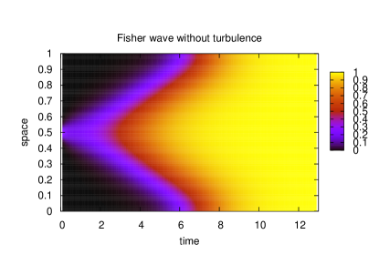
Figure 1: Numerical simulation of eq. 1 with $\mu=1$, $D=0.005$ and with periodic boundary conditions. The initial conditions are $c(x,t)=0$ everywhere expect for few grid points near $L/2=0.5$ where $c=1$. The horizontal axis represents time while the vertical axis is space. The colors display different contour levels of $c(x,t)$.

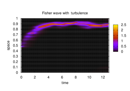
Figure 2: Same parameters and initial condition as in Fig. (1) for equation (3) with a ”strong turbulent” flow $u$ advecting $c(x,t)$.

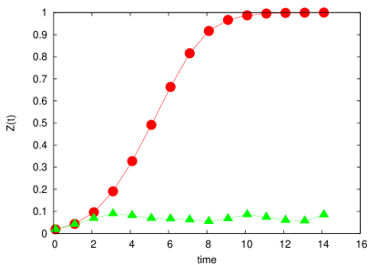
Figure 3: The behavior in time of the total ”mass” $Z(t)\equiv\int dxc(x,t)$. The red circles show the function $Z$ for the case of Fig. (1), i.e. a Fisher wave with no turbulence. The green triangles show $Z$ for the case of Fig. (2) when a strong turbulent flows is advecting $c(x,t)$.

With biological applications in mind, it is important to determine conditions such that the spatial distribution of microbial organisms and the carrying capacity of the medium are significantly altered by convective turbulence. Within the framework of the Fisher equation, localization effect has been studied for a constant convection velocity and quenched time-independent spatial dependence in the growth rate $\mu$ [6], [7], [12], [13]. In our case, localization, when it happens, is a time-dependent feature and depends on the statistical properties of the compressible turbulent flows. As discussed in detail below, a better term for the phenomenon we study here might be ”quasilocalization”, in the sense that (1) spatial localization of the growing population sometimes occurs at more than one location; (2) these spatial locations drift slowly about and (3) localization is intermittent in time, as localized populations collapse and then reform elsewhere. For these reasons, the quasilocalization studied here is not quite the same phenomena as the Anderson localization of electrons in a disordered potential studied in [16]. Nevertheless, the similarities are sufficiently strong that we shall use the terms ”quasilocalization” and ”localization” interchangeably in this paper. It is worth noting that the localized ”boom and bust” population cycles studied here may significantly effect ”gene surfing” [14] at the edge of a growing population, i.e. by changing the probability of gene mutation and fixation in the population.

For the case of bacterial populations subject to both turbulence and convections due to, say, an external force such as sedimentation under the action of gravity, we may think that the turbulent velocity can be decomposed into a constant ”wind” $u_{0}$ and a turbulent fluctuation $u(x,t)$ with zero mean value, $U(x,t)=u_{0}+u(x,t)$. We find that the localization shown in Fig. (2) can be significantly changed for large enough background convection $u_{0}$.

We would like to understand why and how $u_{0}\neq 0$ can change the statistical properties of $c(x,t)$ in the presence of a random convecting velocity field. We wish to understand, in particular, whether $c(x,t)$ spreads or localizes as a function of parameters such as the turbulence intensity and the mean ”wind” speed $u_{0}$.

Our results are based on a number of numerical simulations of Eq. (3) performed using a particular model for the fluctuating velocity field $u(x,t)$. In Sec. $1$ we introduce the model and we describe some details of the numerical simulations. In Sec. $2$ we develop a simple ”phenomenological” theory of the physics of Eq. (3) based on our present understanding of turbulent dynamics. In Sec. $3$ we analyze the numerical results when the sedimentation velocity $u_{0}=0$ while in Sec. $4$ we describe our findings for $u_{0}>0$ . Conclusions follow in Sec. $5$.

1 The model

To completely specify equation (3) we must define the dynamics of the ”turbulent” velocity field $U(x,t)$. For now, we set $U(x,t)=u_{0}+u(x,t)$, neglect the uniform part $u_{0}=0$ and focus on $u(x,t)$. Although we consider a one dimensional case, we want to study the statistical properties of $c(x,t)$ subjected to turbulent fluctuations which are close to thos generated by the three dimensional Navier-Stokes equations. Hence, the statistical properties of $u(x,t)$ should be described characterized by intermittency both in space and in time. We build the turbulent field $u(x,t)$ by appealing to a simplified shell model of fluid turbulence [15]. The wavenumber space is divided into shells of scale $k_{n}=2^{n-1}k_{0}$, $n=1,2,...$. For each shell with characteristic wavenumber $k_{n}$, we describe turbulence by using the complex Fourier-like variable $u_{n}(t)$, satisfing the following equation of motion:

$$(\frac{d}{dt} + \nu k_{n}^{2})u_{n}=i(k_{n+1}u_{n+1}^{*}u_{n+2}-\delta k_{n}u_{n-1}^{*}u_{n+1}$$ (4)

$$+ (1-\delta)k_{n-1}u_{n-1}u_{n-2})+f_{n}\ .$$

The model contains one free parameter, $\delta$, and it conserves two quadratic invariants (when the force and the dissipation terms are absent) for all values of $\delta$. The first is the total energy $\sum_{n}|u_{n}|^{2}$ and the second is $\sum_{n}(-1)^{n}k_{n}^{\alpha}|u_{n}|^{2}$, where $\alpha=\log_{2}(1-\delta)$. In this note we fix $\delta=-0.4$. For this value of $\delta$ the model reproduces intermittency features of the real three dimensional Navier Stokes equation with surprising good accuracy [15]. Using $u_{n}$, we can build the real one dimensional velocity field $u(x,t)$ as follows:

$$u(x,t)=F\sum_{n}[u_{n}e^{ik_{n}x}+u^{*}_{n}e^{-ik_{n}x}],$$ (5)

where $F$ is a free parameter to tune the strength of velocity fluctuations (given by $u_{n}$) relative to other parameters in the model (see next section). In all numerical simulations we use a forcing function $f_{n}=(\epsilon(1+i)/u^{*}_{1})\delta_{n,1}$, i.e. energy is supplied only to the largest scale corresponding to $n=1$. With this choice, the input power in the shell model is simply given by $1/2\sum_{n}[u^{*}_{n}f_{n}+u_{n}f^{*}_{n}]=\epsilon$ , i.e. it is constant in time. To solve Eqs. (3) and (4) we use a finite difference scheme with periodic boundary conditions.

Theses model equations can be studied in detail without major computational efforts. One main point of this note is to explore the qualitative and quantitative dynamics of Eqs. (3),(4) and compare it against the phenomenological theory developed in the next section.

The free parameters of the model are the diffusion constant $D$, the size of the periodic 1d spatial domain $L$, the growth rate $\mu$, the viscosity $\nu$ (which fixes the Reynolds number $Re$), the mean constant velociy $u_{0}$, the “strength’ of the turbulence $F$ and finally the power input in the shell model, namely $\epsilon$. Note that according to the Kolmogorov theory [11], $\epsilon\sim u_{rms}^{3}/L$ where $u_{rms}^{2}$ is the mean square velocity. Since $u_{rms}\sim F$, we obtain that $F$ and $\epsilon$ are related as $\epsilon\sim F^{3}$. By rescaling of space, we can always put $L=1$. We fix $\epsilon=0.04$ and $\nu=10^{-6}$, corresponding to an equivalent $Re=u_{rms}L/\nu\sim 3\times 10^{5}$. As we shall see in the following, most of our numerical results are independent of $Re$ when $Re$ is large enough. In the limit $Re\rightarrow\infty$, the statistical properties of eq. (3) depend on the remaining free parameters, $D$, $u_{0}$, $\mu$ and $F$. The important combinations of these parameters are discussed in the next section.

2 Theoretical considerations

We start our analysis by rewriting (3) in the form:

$$\partial_{t}c+(u_{0}+w)\partial_{x}(c)=D\partial_{x}^{2}c+(\mu+g)c-bc^{2}$$ (6)

where $w\equiv u(x,t)$ and $g(x,t)\equiv-\partial_{x}u(x,t)$. Previous theoretical investigations [6] have shown that for $u_{0}=w=0$, $c(x,t)$ becomes localized in space for time-independent ”random” forcing $g=g(x)$ (Anderson localization [16]). For $u_{0}$ large enough, a transition from localized to extended solutions has been predicted and observed in previous numerical and theoretical works [12]. Here, we wish to understand whether something resembling localized solutions survives in equation (6) when both $w$ and $g$ depend on time as well as space.

To motivate our subsequent analysis, consider first the case $\mu=u_{b}=0$. In this limit, Eq. (3) is just the Fokker-Planck equation describing the probability distribution $P(x,t)\equiv c(x,t)$ to find a particle in the range $(x,x+dx)$ at time $t$, whose dynamics is given by the stochastic differential equation:

$$\frac{dx}{dt}=u(x,t)+\sqrt{2D}\eta(t)$$ (7)

where $\eta(t)$ is a white noise with $\langle\eta(t)\eta(t^{\prime})\rangle=\delta(t-t^{\prime})$. Let us assume for the moment that $u(x,t)=u(x)$ is time independent. Then, the stationary solution of (3) is given by

$$P(x,t)=A^{-1}exp[-\Phi(x)/D]$$ (8)

where $A$ is a normalization constant and $\partial_{x}\Phi=-u(x)$. It follows that $P(x,t)=P(x)$ is strongly peaked near the points $x_{i}$ where $\Phi$ has a local minimum, i.e. $u(x_{i})=0$ and $-\partial^{2}_{xx}\Phi\equiv\partial_{x}u(x)|_{x=x_{i}}<0$. Let us now consider the behaviour of $P(x)$ near one particular point $x_{0}$ where $u(x_{0})=0$. For $x$ close to $x_{0}$ we can write:

$$\frac{dx}{dt}=-\Gamma_{0}(x-x_{0})+\sqrt{2D}\eta(t)$$ (9)

where $\Gamma_{0}\equiv-\partial_{x}u(x)|_{x=x_{0}}$. Equation (9) is the Langevin equation for an overdamped harmonic oscillator, and tells us that $P$ is spread around $x_{0}$ with a characteristic ”localizaiont length” of order $\xi_{l}\equiv\sqrt{D/\Gamma_{0}}$. On the other hand, we can identify $\Gamma_{0}$ with $\Gamma$, a typical gradient of the turbulent velocity field $u$. In a turbulent flow, the velocity field is correlated over spatial scale of order $v_{*}/\Gamma$ where $v_{*}^{2}/2$ is the average kinetic energy of the flow. For $P$ to be localized near $x_{0}$, despite spatial variation in the turbulent field, we must require that the localization length $\xi_{l}$ should be smaller than the turbulent correlation scale $v_{*}/\Gamma$, i.e.

$$\sqrt{\frac{D}{\Gamma}}<\frac{v_{*}}{\Gamma}\rightarrow\frac{v_{*}^{2}}{D\Gamma}>2$$ (10)

Condition (10) can be easily understood by considering the simple case of a periodic velocity field $u$, i.e. $u=v_{*}cos(xv_{*}/\Gamma)$. In this case, condition (10) states that $D$ should be small enough for the probability $P$ not to spread over all the minima of $u$. For small $D$ or equivalently for large $v_{*}^{2}/\Gamma$, the solution will be localized near the minima of $u$, at least for the case of a frozen turbulent velocity field $u(x)$.

The above analysis can be extended for velocity field $u(x,t)$ that depend on both space and time. The crucial observation is that, close to the minima $x_{i}$ of $\Phi(x,t)\equiv-\int dxu(x,t)$, we should have $u(x_{i},t)\sim 0$. Thus, although $u$ is a time dependent function, sharp peaks in $P(x,t)$ move quite slowly, simply because $u(x,t)\sim 0$ near the maximum of $P(x,t)$. One can consider a Lagrangian path $x(t)$ such that $x(0)=x_{0}$, where $x_{0}$ is one particular point where $u(x_{0},0)=0$ and $\partial_{x}u(x,0)|_{x=x_{0}}<0$. From direct numerical simulation of Lagrangian particles in fully developed turbulence, we know that the acceleration of Lagrangian particles is a strongly intermittent quantitiy, i.e. it is small most of the time with large (intermittent) bursts. Thus, we expect that the localized solution of $P$ follows $x(t)$ for quite long times except for intermittent bursts in the turbulent flow. During such bursts, the position where $u=0$ changes abruptly, i.e. almost discontinuosly from one point, say $x(t)$, to another point $x(t+\delta t)$. During the short time interval $\delta t$, $P$ will drift and spread, eventually reforming to become localized again near $x(t+\delta t)$. The above discussion suggests that the probability $P(x,t)$ will be localized most of the time in the Lagrangian frame, except for short time intervals $\delta t$ during an intermittent burst.

We now revisit the condition (10). For the case of a time-dependent velocity field $u$, we estimate $\Gamma$ as the characteristic gradient of the velocity field, i.e.

$$\Gamma\sim\langle(\partial_{x}u)^{2}\rangle^{1/2}$$

where $\langle..\rangle$ stands for a time average. Now, $v_{*}^{2}$ should be considered as the mean kinetic energy of the turbulent fluctuations. In our model, both $v_{*}$ and $\Gamma$ are proportional to $F$, the strength of the velocity fluctuations. Thus, we can rewrite the localization criteria (10) in the form:

$$\frac{v_{*}^{2}F}{D\Gamma}>2$$ (11)

where $v_{*}$ and $\Gamma$ are computed for $F=1$. We conclude that for small values of $F$, $P(x,t)$ is spread out, while for large $F$, $P$ should be a localized or sharply peaked function of $x$ most of the time. An abrupt transition, or at least a sharp crossover, from extended to sharply peaked functions $P$, should be observed for increasingf $F$.

It is relatively simple to extend the above analysis for a non zero growth rate $\mu>0$. The requirement (10) is now only a necessary condition to observe localization in $c$. For $\mu>0$ we must also require that the characteristic gradient on scale $\xi_{l}$ must be larger than $\mu$, i.e. the effect of turbulence should act on a time scale smaller than $1/\mu$. We estimate the gradient on scale $\xi_{l}$ as $\delta v(\xi_{l})/\xi_{l}$, where $\delta v(\xi_{l})$ is the characteristic velocity difference on scale $\xi_{l}$. We invoke the Kolmogorov theory, and set $\delta v(\xi_{l})=v_{*}(\xi_{l}/L)^{1/3}$ to obtain:

$$\mu<\frac{\delta v(\xi_{l})}{\xi_{l}}=\frac{v_{*}\xi_{l}^{-2/3}}{L^{1/3}}=v_{*}(\frac{\Gamma}{LD})^{1/3}$$ (12)

In (12), we interpret $\Gamma$ as the characteristic velocity gradient of the turbulent flow. Because $v_{*}\sim F$ and $\Gamma\sim F$, it follows that the r.h.s of (12) goes as $F^{4/3}$. Note also that $\delta v(\xi_{l})/\xi_{l}\leq\Gamma$ on the average, which leads to the inequality:

$$\mu<\Gamma$$ (13)

From (10) and (13) we also find

$$\frac{v_{*}^{2}}{D\mu}>2$$ (14)

a second necessary condition. Once again, we see that localization in a Lagrangian frame should be expected for strong enough turbulence.

One may wonder whether a non zero growth rate $\mu$ can change our previous conclusions about the temporal behavior, and in particular about its effect on the dynamics of the Lagrangian points where $u(x,t)=0$. Consider the solution of (3) at time $t$, allow for a spatial domain of size $L$, and introduce the average position

$$x_{m}\equiv\int_{0}^{L}dxx\frac{c(x,t)}{Z(t)}$$ (15)

where $Z(t)=\int_{0}^{L}dxc(x,t)$. Upon assuming for simplicity a single localized solution, we can think of $x_{m}$ just as the position where most of the bacterial concentration $c(x,t)$ is localized. Using Eq. (3), we can compute the time derivative $v_{m}(t)=dx_{m}/dt$. After a short computation, we obtain:

$$v_{m}(t)=Z\int_{0}^{L}dx(x_{m}-x)P(x,t)^{2}+\int_{0}^{L}u(x,t)P(x,t)dx$$ (16)

where $P(x,t)\equiv c(x,t)/Z(t)$ and $Z(t)=\int_{0}^{L}c(x,t)dx$. Note that $v_{m}$ is independent of $\mu$. Moreover, when $c$ is localized near $x_{m}$, both terms on the r.h.s. of (16) are close to zero. Thus, $v_{m}$ can be significantly different from zero only if $c$ is no longer localized and the first integral on the r.h.s becomes relevant. We can now understand the effect of the non linear term in (3): when $c(x,t)$ is localized, the non linear term is almost irrelevant simply because $v_{m}$ is close to $0$. On the other hand, when $c(x,t)$ is extended the non linear term drives the system to the state $c=1$ which is an exact solution in the absence of turbulent convection $u(x,t)=0$.

We now allow a non zero mean flow $u_{0}\neq 0$. As before, we first set $\mu=b=0$ and consider a time -independent velocity field $u(x)$. Since the solution $c(x,t)$ of (3) can still be interpreted as be the probability to find a particle in the interval $[x,x+dx]$ at time $t$, we can rewrite (9) for the case $u_{0}>0$ as follows:

$$\frac{dx}{dt}=-\Gamma_{0}(x-x_{0})+u_{0}+\sqrt{2D}\eta(t)$$ (17)

The solution of (3) is localized near the point $x_{1}=x_{0}+u_{0}/\Gamma_{0}$. Thus for small $u_{0}$ or large $\Gamma_{0}$ there is no major change in the arguments leading to (10). In general, we expect that $P(x)$ will be localized near $x=x_{0}$, provided the length $\xi_{0}\equiv|x_{1}-x_{0}|=u_{0}/\Gamma_{0}$ is smaller than $\xi_{l}$, i.e.

$$\frac{u_{0}}{\Gamma_{0}}<\sqrt{\frac{D}{2\Gamma_{0}}}\rightarrow\frac{u_{0}^{2}}{D\Gamma_{0}}<2$$ (18)

When (18) is satisfied, then our previous analysis on localized solutions for both $\mu=0$ and $\mu\neq 0$ is still valid. Let us note that by combing (13) and (18) we obtain

$$\frac{u_{0}^{2}}{D\mu}<2$$ (19)

as a condition for localization, obtained in the study of localized/extended transition for steady flowsin an Eulerian context [7], [12]. Here we remark that in a turbulent flow, Eq. (19) is only a necessary condition, because (10),(12) and (18) must all also be satisfied for $c$ to show quasi-localized states.

To study the change in the spatial behaviour of $P$ as a function of time, we need a measure of the degree of localization. to look for an some kind of order parameter. Although there may be a number of valuable solutions, an efficient measure should be related to the ”order”/”disorder” features of $c(x,t)$, where ”order” means quasi-localized and ”disorder” extended. As pointed out in the introduction, the total ”mass” of the organisms $Z(t)\equiv\int_{0}^{L}dxc(x,t)$ is strongly affected by a strongly peaked (or quasi-localized) $c(x,t)$, as opposed to a more extended concentration field. However, a more illuminating quantity, easily studied in simulations, is

$$S(t)=-\int_{0}^{L}dxP(x,t)log(P(x,t))$$ (20)

where $P(x,t)\equiv c(x,t)/Z$. Localized solutions of Eq. (3) correspond to small values of this entropy-like quantity while extended solutions correspond to large values of $S$, which can be interpreted as the information contained in the probability distribution $P(x,t)$ at time $t$. In our numerical simulations, we consider a discretized form of (20), namely:

$$S(t)=-\sum_{i=1,N}\frac{c(x_{i},t)}{Z}log(\frac{c(x_{i},t)}{Z})$$ (21)

where $x_{i}$ are now the $N$ grid points used to discretize (3), $c(x_{i},t)$ is the solution of (3) in $x_{i}$ at time $t$ and $Z(t)\equiv\sum_{i}c(x_{i},t)$.

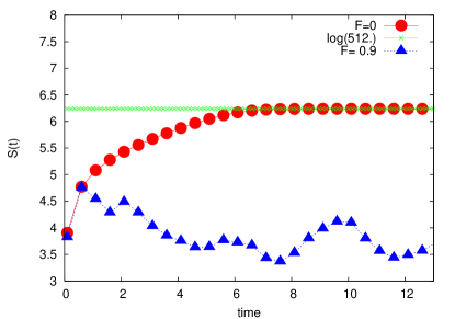
Figure 4: The behavior in time of $S(t)$ . The red circles show the function $S(t)$ for the case of Fig. (1), i.e. a Fisher wave with no turbulence. The blue triangles show $S(t)$ for the case of Fig. (2) when a ”strong” turbulent flows is advecting $c(x,t)$.

To understand how well $S(t)$ describes whether $c(x,t)$ is localized or extended, we consider the cases discussed in the Introduction in Fig.s (1) and (2). The numerical computations were done with $F=0$ for Fig. (1) and $F=0.9$ for Fig. (2), i.e. no turbulence and ”strong” turbulence (the attribute ”strong” refers to the conditions (10) and (12). In Fig. (4) we show $S(t)$ corresponding to the two simulations, namely $F=0$ (red circles) and $F=0.9$ (blue triangles). The initial condition is the same for both simulations $c(x,0)=exp[-(x-L/2)^{2}/0.05]$, i.e. a rather localized starting point. It is quite clear, from inspecting Fig. (4), that $S(t)$ is a rather good indicator to detect whether $c(x,t)$ remains localized or becomes extended. While for $F=0$ (a quiescent fluid), $S$ reaches its maximum value( $S=9log(2.)$ for $512$ grid points) at $t=6.$ (corresponding to uniform concentration $c(x,t)=1$), for $F=0.9$, $S$ is always close to its initial value $S\sim 4.$, indicating that $c(x,t)$ is localized, in agreement with Fig. (2).

Let us summarize our findings: when subjected to turbulence, we expect $c(x,t)$ to be ”localized”, i.e. strongly peaked, most of the time for large enough $F$ and $u_{0}=\mu=b=0$. Upon increasing the growth rate $\mu$, the value of $F$ where $c(x,t)$ shows Lagrangian localization should increase. Finally, for fixed $F$ and $\mu$ we should find a localized/extended crossover for large enough values of $u_{0}$. Because our theoretical analysis is based on scaling arguments, we are not able to fix the critical values for which localized/extended transition should occour as a function of $D$,$F$ and $u_{0}$. However, we expect that the conditions (10),(12) and (18) capture the scaling properties in the parameter space of the model. Finally, we have introduced an entropy like quantity $S(t)$ useful for analyzing the time dependence of of $c(x,t)$ and for distinguishing between localized and extended solutions. In the following section, we compare our theoretical analysis against numerical simulations.

3 Numerical results for $u_{0}=0$

We now discuss numerical results obtained by integrating equation Eq. (3). As discussed in Sec. $1$, all numerical simulations have been done using periodic boundary conditions. Eq. (3) has been discretized on a regular grid of $N=512$ points. Changing the resolution $N$, shifting $N$ to $N=1024$ or $N=128$, does not change the results discussed in the following. We use the same extended initial condition $c(x,t)=1$ for all numerical simulations with the few exceptions which discussed in the introduction (the Fisher wave) and in the conclusions. For all simulations studied here, the diffussion constant $D$ has been kept fixed at $D=0.005$.

We first discuss the case $\mu=b=0$ term and beginby understanding how well $S(t)$ describes the localized/extended feature of the $c(x,t)$. In Fig. (5) we plot $S(t)$ as a function of time for a case with $F=0.5.$. The behaviour of $S(t)$ is quite chaotic, as expected. In Fig. (6) we show the functions $c(x,t)$ for two particular times, namely $t=35.$ (lower panel) and $t=60$ (upper panel). These two particular configurations correspond to extended ($t=35$) and quasi-localized ($t=60$) solutions. The corresponding values of $S$ are $S=5.5$ for $t=35.$ and $S=3.5$ for $t=60$. It is quite clear that for small $S$ strong localization characterizes $c(x)$ while for increasing $S$ the behaviour of $c(x)$ is more extended.

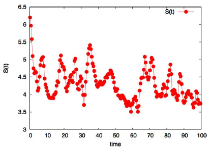
Figure 5: The behavior of $S(t)$ for a numerical simulation of (3) for $\mu=b=u_{0}=0$, no saturation term $c^{2}(x.t)$ and $F=0.5$. With our uniform initial condition, $S(0)=9log(2.)$. As discussed in Sec. 2, $S(t)$ is a reasonable indicator for localized/extended spatial behavior of $c(x,t)$. Since the flow is turbulent, $S(t)$ behaves chaotically. However, it fluctuates at values lower that $S(t=0)$ and indicates the degree of localization.

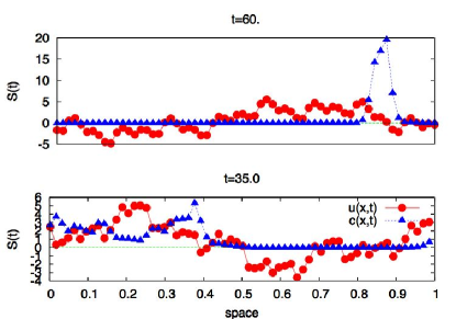
Figure 6: Numerical simulation of Eq. (3) for $\mu=u_{0}=b=0$, term and $F=0.5.$. The upper panel shows $c(x,t)$ (blue triangles) and $u(x,t)$ (red circles) multiply by $10$, at $t=60.$. The lower panel shows the same quantities at $t=35.$. The two time frames have been chosen to illustrate localized (upper panel) and more extended (lower panel) solutions. Note that the localized solution at $t=60.$ reaches its maximum value for $u=0$ and $\partial_{x}u|_{u=0}<0$, as predicted by the analysis of sec. $2$.

In Fig. (6) we also show (red circles) the instantaneous behavior of $u(x,t)$ (multiply by a factor $10$ to make the figure readable). As one can see, the maximum of $c(x,t)$ always corresponds to points where $u=0$.

To understand whether the analysis of Sec. 2 captures the main features of the dynamics. we plot in FIg. (7), for $t=35$ (lower panel) and $t=60$ (upper panel), the quantity $P(x,t)$ as computed from Eq. (8), i.e. by using the instantaneous velocity field $u(x,t)$. Although there is a rather poor agreement between $c(x,t)$ and $P(x,t)$ at $t=35$, at time $t=60$ the $P(x,t)$ is a rather good approximation of $c(x,t)$, i.e. when $c(x,t)$ is localized. The spatial behavior of $c(x,t)$ is dictated by the point $x_{0}$ where $u=0$ and the velocity gradient $\partial u|_{x=x_{0}}$ is large and negative. All the above results are in qualitative agreement with our analysis.

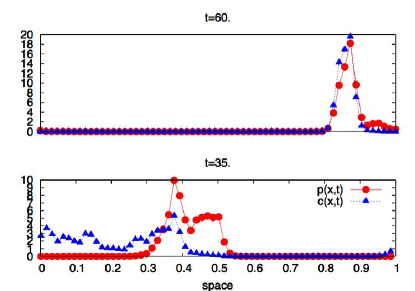
Figure 7: Numerical simulation of (3) for $\mu=b=u_{0}=0$ and $F=0.5.$. The upper panel shows $c(x.t)$ (red circles) at $t=60.$and the behavior of $P(x,t)$ (blue triangle) computed using (8) using the instantaneous velocity field shown in Fig. (6). In the lower panel we show the same quantities ($c(x,t)$ and $P(x,t)$) at time $f=35.$ when the solution is extended.

Next we test the condition (11), which states that localization should become more pronounced for increasing values of $F$. To test Eq. (11) we performed a number of numerical simulations with long enough time integration to reach statistical stationarity. In Fig. (8) we show $\langle S\rangle$ as function of $F$, where $\langle...\rangle$ means a time average. In the insert of the same figure, we show to time dependence of $S(t)$ for two different values of $F$, namely $F=0.4$ and $F=1.8$. The behavior of $\langle S\rangle$ is decreasing as a function of $F$, in agreement with (11). The temporal behavior of $S$, for two individual realizations shown in the insert, reveals that, while on the average $S$ decreases for increasing $F$, there are quite large oscillations in $S$, i.e. the system shows both localized and extended states during its time evolution. However, for large $F$ localization is more pronounced and frequent. On the other hand, for small values of $F$, localization is a ”rare” event. Overall, the qualitative picture emerging from Fig. (8) is in agreement with Eqs. (10) and (11)

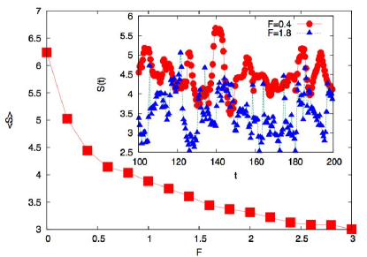
Figure 8: Time averaged entropy $\langle S\rangle$ as a function of $F$. For large $F$ the system fluctuates about small values of $S$,i.e. $c(x,t)$ becomes more localized. In the insert, we show the time behaviour of $S(t)$ for two particular values of $F$, namely $F=0.4$ (red curve) and $F=1.8$ (blue curve). Numerical simulations performed for $\mu=b=u_{0}=0$

In the previous section we argued that (10) and (11) apply also for a time-dependent function velocity $u(x,t)$. The basic idea was that $c(x,t)$ is localized near some point $x_{0}$ which slowly changes in time, except for intermittent bursts. In sufficiently large systems, localization about multiple points is possible as well. During the intermittent burst, $c(x,t)$ spreads and after the burst $c(x,t)$ becomes localized around a new position $x_{0}$. We have already shown, in Figs. (6) and (7), that our argument seems to be in agreement with the numerical computations using a time-dependent velocity field. To better understand this point, we measure $v_{m}$ defined in Eq. (16). We expect a small $v_{m}$ during localized epochs when $S$ is small. Each time interval when $c$ is localized, should end and start with an intermittent burst where $|v_{m}|$ may become large. Figs (9) illustrates the above dynamics. The solid red curve is $v_{m}(t)$ multiplied by a factor $10$ while the blue dotted curve shows $S(t)$. The numerical simulation is for $F=2.$, i.e. to a case where localization is predominant in the system. Fig. (9) clearly shows the ”intermittent” bursts in the velocity $v_{m}$. The stagnation point velocity, punctuated by large positive and negative excursions, typically wanders near $0$. If we assume a single sharp maximum in $c(x,t)$, as in the upper panel of Fig. (6), the localized profile $c(x,t)$ does not move or moves quite slowly. During an intermittent burst, $v_{m}$ grows significantly while $c(x,t)$ spreads over the space. Soon after the intermittent burst (see for instance the snapshot at time $t=15$ in Fig. (9)), the velocity $v_{m}$ becomes small again and the corresponding value of $S$ decreases. Fig. (9) provides a concise summary of the dynamics: both localized and extended configurations of $c(x,t)$ are observed as a function of time. During a era of localization, a bacterial concentration described by $c(x,t)$ is in a kind of ”quasi-frozen” configuration.

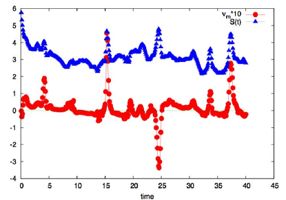
Figure 9: Time dependence of $v_{m}$ (red curve) and $S(t)$ (blue curve) for $F=2.0$. The value of $v_{m}$ is multiplied by $10$ to make the figure readable. The velocity of the accumulation point for the bacterial concentration $c(x,t)$, $v_{m}$ , is computed using (16). We again set $\mu=u_{0}=b=0$.

Fig. (9) tells us that condition (10), which was derived initially for a frozen turbulent field $u$, works as well for time dependent turbulent fluctuations. As $F$ increases, the system undergoes a sharp crossover and the dynamics of $c(x,t)$ slows down in localized configurations. Additional features of this transition will be discussed later on when we focus on a quantity analogous to the specific heat.

Finally in Fig. (10) we show the probability distribution $P(S)$, obtained by the numerical simulations, for three different values of $F$, namely $F=0.2,0.8$ and $F=2.$. As one can see, the maximum $P(S)$ is shifted toward small values of $S$ for increasing $F$, as we already know from Fig. (8). Fig. (10) shows that the fluctuations of $S$ about the mean are approximately independent of $F$.

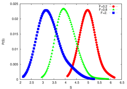
Figure 10: Probability distribution $P(S)$ of ”entropy” $S$ defined by (21), obtained by the numerical simulations, for three different values of $F$, namely $F=0.2,0.8$ and $F=2.$.

We now turn our attention to the case $\mu>0$ . We have performed numerical simulations for two growth rates, namely $\mu=1$ and $\mu=5$. We start by analyzing the results for $\mu=1$. In Fig. (11), we show the behaviour of $\langle S\rangle$ as a function of $F$, while in the insert we show the probability distribution $P(S)$ for three values of $S$. Upon comparing with Fig. (11) against Fig.s (8) and (10), we see that a nonzero growth rate $\mu=1$ does not change the qualitative behavior of the system, in agreement with our theoretical discussions in the previous section.

It is interesting to look at the time averaged bacterial mass $\langle Z\rangle$ as a function of $F$. In Fig. (11) we show $\langle Z\rangle$ and $\langle S\rangle/S_{max}$ as a function of $F$. For large $F$, when localization dominates the behavior of $c(x,t)$, $\langle Z\rangle$ is quite small, order $0.1$ of its maximum value, i.e. due to turbulence the population $c(x,t)$ only saturates locally at a few isolated points. The reduction in $\langle Z(t)\rangle$ tracks in $\langle S(t)\rangle$, but is much more pronounced.

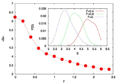
Figure 11: Computation of $\langle S\rangle$ as a function of $F$ for $\mu=1$. In the insert, we show the prrobability distribution $P(S)$, obtained by the numerical simulations, for three different values of $F$, namely $F=0.4,0.8$ and $F=2.$

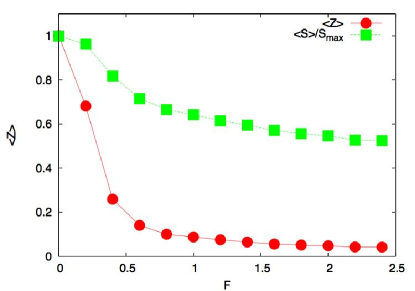
Figure 12: Computation of the total bacterial mass $\langle Z\rangle$ (normalized to $1$ at $F=0$) for $\mu=1$ (red circles) and of $\langle S\rangle/S_{max}$ (green squares) as a function of $F$

In Fig. (13) we show $v_{m}(t)$ computed for the case $\mu=1$ and $F=3.$. As in Fig. (9), we plot $v_{m}*10$ and $S(t)$. The qualitative behaviour is quite close to what already discussed for the case $\mu=b=0$. The whole picture for $\mu=1$, as obtained by inspection of Fig.s (11) and (13), supports our previous conclusions that, as long as the systems is in a quasi-localized phase, the effect of $\mu$ in Eq. (3) is almost irrelevant. Note that for the system to be in the localized phase we must require that both conditions (11) and (12) must be satisfied.

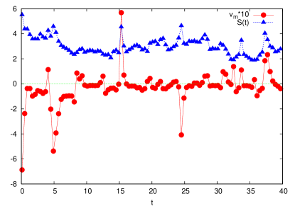
Figure 13: Same as in Fig. (9) for $\mu=1$, non zero saturation term and $F=3.0$.

According to our interpretation, we expect that for increasing $\mu$ the whole picture does not change provided $F$ is increased accordingly. More precisely, we expect that the relevant physical parameters are dictated by the ratios in Eqs. (11) and (12). To show that this is indeed the case, we show in Fig. (14) the results corresponding to those in Fig. (11) but now with $\mu=5$ instead of $\mu=1$.

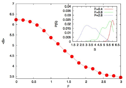
Figure 14: Same as in Fig. (11) for $\mu=5$.

Two clear features appear in Fig. (14). First the qualitative behavior of $\langle S\rangle$ with increasing $F$ is similar for $\mu=5$ and $\mu=1$. This similarity also applies to the probability distribution $P(S)$ shown in the insert of Fig. (14). Second, there is a shift of the function $\langle S\rangle_{F}$ towards large values of $F$, i.e. the localized/extended transition occurs for larger values of $F$ with respect to the case $\mu=1$. This trend is in qualitative agreement with the condition (12).

To make progress towards a quantitative understanding, we would like to use (10) and (12) to predict the shift in the localized/extended transition (or crossover) for increasing $\mu$. For this purpose, we need a better indicator of this transition. So far, we used $S$ as a measure of localization: large values of $S$ mean extended states while small values of $S$ imply a more sharply peaked probability distribution. For $\mu=b=0$, $S$ is the ”entropy” related to the probability distribution $P(x,t)$, solution of eq. (3). Thus for $\mu=b=0$ we can think of $S$ as the ”entropy” and of the diffusion constant $D$ as the ”temperature” of our system. This analogy suggests we define a ”specific heat” $C_{s}=D\partial S/\partial D$ of our system in terms of $S$ and $D$. After a simple computation we get using equations (8) and (20):

$$C_{s}(t)=\int_{0}^{L}dxP(x,t)[log(P(x,t))-\int_{0}^{L}dxP(x,t)log(P(x,t))]^{2}$$ (22)

After allowing a statistically stationary state to develop, we then compute the time average $\langle C_{s}\rangle$ to characterize the ”specific heat” of our system for a specific value of $F$. It is now tempting to describe the localized/extended changeover associated with (3) in terms of the ”thermodynamical” function $\langle C_{s}\rangle$. In other words, we would like to understand whether a change in the specific heat can be used to ”measure” the extended/localized transition with increasing $F$. The above analysis can be done also for $\mu>0$ , (when $c(x,t)$ is no longer conserved) by using $P(x,t)\equiv c(x,t)/Z$ where the ”partition function” $Z(t)=\int_{0}^{L}dxc(x,t)$.

In Fig. (15) we show $\langle C_{s}\rangle$ as a function of $F$ for $\mu=1$ (red curve with circles) and $\mu=5$ (green thin curve). Two major features emerge form this figure. First, $\langle C_{s}\rangle$ is almost $0$ for small $F$ i.e. in the extended case. In the vicinity of a critical value $F=F_{c}$, $\langle C_{s}\rangle$ shows a rapid rise to large positive values and it stays more or less constant upon increasing $F$. The large value of $\langle C_{s}\rangle$ reflects enhanced fluctuations in $log(P(x,t))$ (analogous to energy fluctuations in equilibrium statistical mechanics) when the population is localized. This behavior is in qualitative agreement with the notion of phase transition where (within mean field theory) the specific heat rises after a transition to an ”ordered state”. Here, the ”ordered state” corresponds to a quasilocalized, or sharply peaked probability distribution $P(x,t)$. Our numerics cannot, at present, distinguish between a rapid crossover and a sharp phase transition.

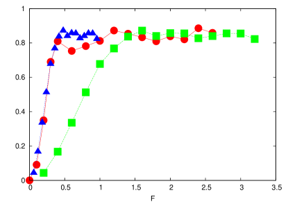
Figure 15: $\langle C_{s}\rangle$ as a function of $F$ for $\mu=1$ (red curve with circles) and $\mu=5$ (green thin curve). The blue line with triangles is $\langle C_{s}\rangle$ for $\mu=5$ plotted against $F/5^{3/4}$, for reasons discussed in the text.

The second interesting feature emerging from Fig. (15) is that $F_{c}$, the value of $F$ corresponding to the most rapid arise of $\langle C_{s}\rangle_{F}$, depends on $\mu$, as predicted by our theoretical considerations. Indeed, as shown just below Eq. (12), we expect that $F_{c}\sim(\mu)^{3/4}$. To check this prediction, we plot in Fig. (15) a third line (the blue line with triangles) which is just $\langle C_{s}\rangle$ for $\mu=5$ plotted against $F/5^{3/4}$. This rescaling is aimed at matching the position of the extended/localized changeover for the same $F_{c}$ independent of $\mu$. The correspondence between the two curves in Fig. (15) confirms our prediction.

Fig. (15) shows that the statistical properties of $c(x,t)$ can be interpreted in terms of thermodynamical quantities. How far this analogy goes, is left to future research. The quantity $\langle C_{s}\rangle$ is in any case a sensitive measure of the extended/localized transition with increasing $F$.

4 Numerical simulations for $u_{0}\neq 0$.

As discussed in Sec. $2$, for fixed large $F$, a mean background flow $u_{0}\neq 0$ can eventually induce a transition from localized to extended configurations of $c(x,t)$. More precisely, for large $F$, i.e. for $F$ large enough to satisfy (10) and (12), the system will spend most of its time in localized states provided the condition (18) is satisfied. Thus, for large enough $u_{0}$ we expect a transition from quasi localized (i.e. sharply peaked) to extended solutions. In this section we study this transition and check the delocalization condition in (18).

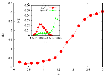
Figure 16: Plot of $\langle S\rangle$ as a function of $u_{0}$ for $\mu=1$ and $F=2.4$. In the insert we show the probability distribution $P(S)$ for two particular values of $u_{0}$, namely $1.$ and $2.2$.

For this purpose we fix $\mu=1$ and $F=2.4$ which, according to our results in the previous section, correspond for $u_{0}=0$ to the case where localized states of $c$ dominate. As before, we use $\langle S\rangle$ and of $P(S)$ to characterize the statistical properties of $c$ for different values of $u_{0}$. In Fig. (16) we show $\langle S\rangle$ as a function of $u_{0}$ while in the insert we show the probability distribution $P(S)$ for two particular values of $u_{0}$. For $u_{0}\sim 2$ we observe a quite strong increase of $\langle S\rangle$ , a signature of a transition from predominately localized to predominately extended states. An interesting feature of $P(S)$ for $u_{0}=2.2$ is the long tail towards small values of $S$. This means that, occasionally, the system recovers a localized concentration distribution, as if $u_{0}=0$.

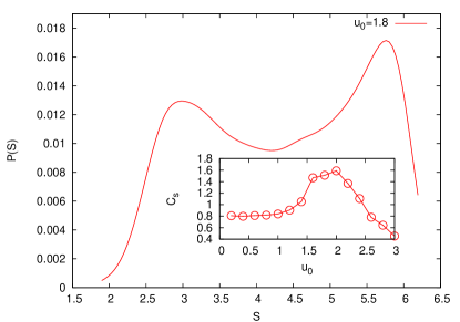
Figure 17: Plot of the probability distribution $P(S)$ for $u_{0}=1.8$, $\mu=1$ and $F=2.4$. In the insert we plot $\langle C_{s}\rangle$ as a function of $u_{0}$, where $C_{s}$ is computed using Eq. (22).

The most striking feature appears near the critical value of $u_{0}$ where the transition a sharp rise in $\langle S\rangle_{u_{0}}$ occurs. In Fig. (17) we show a two-peaked probability distribution $P(S)$ for $u_{0}=1.8$, where the slope of $\langle S\rangle_{u_{0}}$ is the largest, and in the insert we show $\langle C_{s}\rangle$ as a function of $u_{0}$, where $C_{s}$ is computed using Eq.(22). Let us first discuss the result shown in the insert of Fig. (17). The specific-heat like quantity rises form $0.8$ at small $u_{0}$, shows a bump where extended and localized states coexist, and then drops to $0.4$ for $u_{0}$ large. Note that the behavior of $\langle C_{s}\rangle$ is different from what we observe in Fig. (15) suggesting a behavior reminiscent of a first order phase transition. We estimate $u_{0}\sim 1.8$ as the critical value of $u_{0}$ where the behavior changes more rapidly. At $u_{0}=1.8$ the probability distribution is clearly bimodal, i.e. we can detect the two different phases of the system, one characterized by highly localized states and the other characterized by extended states. Turbulent fluctuations drive the system from one state to the other. The two maxima in $P(S)$ are suggestive of two different statistical equilibria of the system. Note that $\langle C_{s}\rangle$ is once again a good indicator of the transition from predominantly localized to predominantly extended states, as discussed in the previous section.

For $u_{0}\neq 0$, a straigthforward generalization of Eq. (16) leads to the following results for the velocity of a maximum in $c(x,t)$,

$$v_{m}=\mu Z\int_{0}^{L}dx(x_{m}-x)P(x,t)^{2}+\int_{0}^{L}u(x,t)P(x,t)dx+u_{0}$$ (23)

One can wonder whether even for $u_{0}>0$, the localized regime of small $S$ shown in Fig. (17) can be still characterized by $v_{m}\sim 0$, thus representing a pinning of the concentration profile despite the drift velocity $u_{0}$. This question is relevant to understand whether the maxima for small $S$ in $P(S)$ shown in Fig. (17) can be described using ideas developed for quasi localized probability distributions in Secs. $2$ and $3$. To answer the above question, we performed a numerical simulation with a time-dependent uniform drift $u_{0}(t)=1.6+0.8*cos(2\pi t/T)$ where $T=10.0$. Thus $u_{0}$ changes periodically in time with an amplitude large enough to drive system from one regime to the other. If our ideas are reasonable, both $S$ and $v_{m}$ will become periodic functions of time. In particular, as $S$l switches from small to large values, $v_{m}$ will go from $0$ in the localized regime to a large positive value in the extended phase.

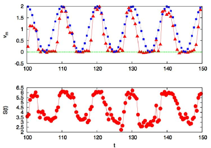
Figure 18: Time dependence of $S(t)$ (lower panel) and $v_{m}(t)$ (upper panel red triangles) for the case of a period mean flow $u_{0}=1.6+0.8cos(2\pi t/T)$ with $T=10$, with the same conditions as in Fig (17). The line with blue squares in the upper panel represents $cos(2\pi t/T)+1$.

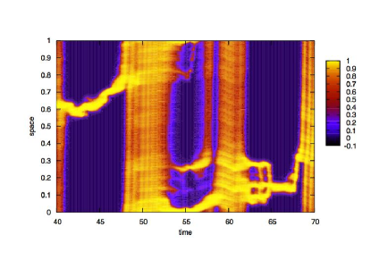
Figure 19: Contour plot of $C(x,t)/Z$ (the horizontal axis is $t$ while the vertical axis is $x$) for the simulation shown in Fig. (18).

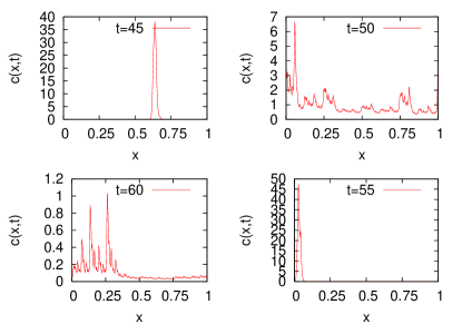
Figure 20: The figure shows four snapshots of $c(x,t)$ taken from FIg. (19) at times $t=45,50,55,60$. At $t=45.$ and $t=55$, when $u_{0}=0.8$, the population $c(x,t)$ is strongly localized while at $t=50$ and $t=60$, when $u_{0}=1.6$, $c(x,t)$ is extended.

Fig. (18) represents a numerical simulation for both $S$ and $v_{m}$. In the upper panel we plot $v_{m}$ (red line) and the periodic function $cos(2\pi t/T)+1$ (we add an offset of $1$ in order to make the figure more readable). As one can see, $v_{m}$ indeed flattens out near periodically in time, and increases to large positive values in synchrony with the external time-dependent drift velocity. In the lower panel, we plot $S$ as a function of time; the graph clearly shows a periodic switching between the two statistical equilibria. A better understanding of the dynamics can be obtained from Fig. (19), where we show a contour plot of the normalized bacterial concentration $c(x,t)/Z$ (the horizontal axis is $t$ while the vertical axis is $x$). Localized states can be observed in the vicinity of $t=45,55$ and $t\sim 65$ i.e when $u_{0}$ is near its smallest value, $u_{0}\sim 0.8$. Localized states are stationary or at most slowly moving whenever $u_{0}$ is small. During the period when $u_{0}$ is large, no localization effect can be observed. Fig. (20) we show four snapshots of $c(x,t)$ taken from FIg. (19) at times $t=45,50,55,60$. At $t=45.$ and $t=55$, when $u_{0}=0.8$, the population $c(x,t)$ is strongly localized while at $t=50$ and $t=60$, when $u_{0}=1.6$, $c(x,t)$ is extended. The reason why $v_{m}\sim 0$ even for a small $u_{0}>0$ is quite simple: according to our analysis in Sec. $2$, localized states will form near shifted zero velocity points with negative slopes even for $u_{0}>0$. When $u_{0}$ is large enough, there is no point where the whole velocity $u(x,t)+u_{0}$ is close to $0$. Every point in the fluid then moves in a particular direction, and the system develops extended states. Fig.s (18), (19) and (20) clearly support this interpretation.

5 Conclusions

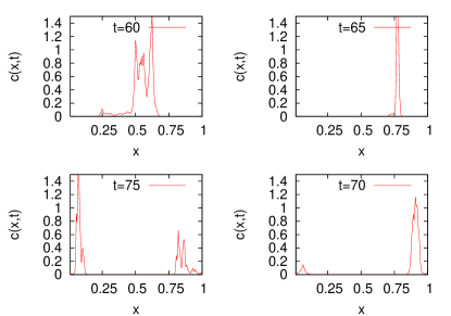
Figure 21: The figure illustrates one of the main results discussed in this paper: the spatial behavior of the population $c(x,t)$ subject to a turbulent velocity field. The figure shows four snapshots of $c(x,t)$ taken from a numerical simulation ($D=0.005$,$\mu=1$, $F=1.2$) at times $t=60,65,70,75$. The population $c(x,t)$ shows strongly peaked concentration at time $t=65$ and $t=70$, while at times $t=65$ and $t=75$, $c(x,t)$ seems to be less peaked. The popultion $c(x,t)$ alternates strongly peaked solutions and more extended ones.

In this paper we have studied the statistical properties of the solution of Eq.(3) for a given one dimnesional turbulent flow $u(x,t)$. Fig. (21) illustrates one of the main results discussed in this paper: the spatial behavior of the population $c(x,t)$ subjected to a turbulent field. In particular, the figure shows four snapshots of $c(x,t)$ taken from a numerical simulation ($D=0.005$, $\mu=1$, $F=1.2$) at times $t=60,65,70,75$. The population $c(x,t)$ shows strongly peaked concentration at time $t=65$ and $t=70$, while at times $t=65$ and $t=75$, $c(x,t)$ is more extended. The popultion $c(x,t)$ alternates strongly peaked solutions and more extended ones Our model is sufficiently simple to allow systematic investigation without major computational effort. From a physical point of view, the model can be interesting for compressible turbulent flows and whenever the field $c$ represents particles (such as the cells of microorganisms) whose numbers grow and saturate while diffusing and advecting. Our aim in this paper was to understand the statistical properties of $c(x,t)$ as a function of the free parameters in the model. We developed in Sec. $2$ a simple theoretical framework. Based on three dimensionless parameters, we have identified three conditions which must be satisfied for quasi localized solutions of (3) to develop, given by Eqs. (10),(12) and (18).

All numerical simulations have been performed by using a grid resolution of $N=512$ points and a Reynolds number $Re\sim 10^{6}$. Increasing the resolution will not change the numerical results provided the appropriate rescaling on conditions (10),(12) and (18) are performed, as shown in the following argument: let us define $\delta x$ the grid spacing, i.e. $\delta x=L/N$, $\eta$ the Kolmogorov scale and $\epsilon$ the mean rate of energy dissipation, where $\eta=(\nu^{3}/\epsilon)^{1/4}$. The turbulent field $u(x,t)$ must be simulated numerically for scales smaller than the Kolmogorov scale. In the shell models, this implies that the largest value of $k_{n}$ is much larger than $1/\eta$. The velocity gradient $\Gamma$ is of the order of $\sqrt{\epsilon/\nu}$. If the grid spacing $\delta x$ is smaller than $\eta$, no rescaling is needed in using the theoretical considerations derived in Sec. $2$, namely equations (10), (12) and (18). On the other hand, if $\delta x$ is larger than $\eta$, as in our simulations, the velocity gradient goes as

$$\Gamma\sim\frac{u(x+\delta x)-u(x)}{\delta x}\sim\epsilon^{1/3}(\delta x)^{-2/3}$$ (24)

Thus, by increasing the resolution, i.e. decreasing $\delta x$, we increase the velocity gradients and the condition (10) may not be satisfied unless we change $D$ or $F$ in an appropriate way. As an example of the above argument we show in Fig. (22) (insert) the value of $\langle C_{s}\rangle$ computed for $N=128$, $D=0.01$ and $\mu=1$ (red line with squares) and compared with the case, used in the main text, $D=0.005$, $N=512$ and $\mu=1$ (green line with circles) already discussed in Sec. 3. For this particular case, we can superimpose the two curves by multiplying $F$ for the $N=128$ case by a factor $0.8$ which comes from equations (10) and (24). The final result agrees quite well with the $N=512$ case as shown in the same figure.

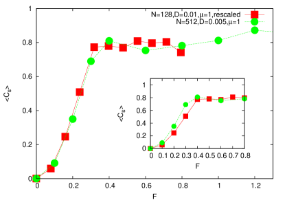
Figure 22: The ”specific heat” $\langle C_{s}\rangle$ computed for $N=128$, $D=0.01$ and $\mu=1$ (red line with squares), rescaled according to (24) and (10), and compared with the case $\mu=1$, $D=0.005$ and $N=512$ (green line with circles) discussed in the text. In the insert the same quantities are plotted without rescaling.

Similar considerations apply for a non zero mean flow $u_{0}$, where the localized/extended transition should occours for larger values of $u_{0}$ according to (18). Finally, let us mention how we can predict the Reynolds number dependence of our analysis. According to the Kolmogorov theory, a typical velocity gradient is $\Gamma\sim Re^{1/2}$. Therefore, the transition from extended to localized solutions predicted by (10) can be observed provided either $D\sim Re^{-1/2}$ or $F\sim Re^{1/2}$. Hence, by increasing the Reynolds number, the extended/localized transition eventually disappears unless the diffusion term $D$ is properly rescaled.

Following the theoretical framework discussed in Sec. $2$, we introduced a simple way to characterized how well $c(x,t)$ is localized in space, namely using the entropy-like function (21) to illuminate the dynamics of the numerical solutions. The time average entropy $\langle S\rangle$ was used to characterize the transition from extended to localized for increasing $F$ and from localized to extended solutions for increasing $u_{0}$. We also found it useful to define a ”specific heat” $C_{s}$ by simply computing $D\partial S/\partial D$, where $D$ plays the role of temperature in the system. Notice from Eq. (10) that the physics is controlled by an effective temperature $D/F$, i.e. rescaling $F$ is equivalent to changing $D$.

The analogy between $F$ and some sort of effective temperature suggests that the rapid rise in the time average $\langle C_{s}\rangle$, observed in Fig. (15) near a characteristic value $F_{c}$, might indicate a critical ”temperature” or diffusion constant $D_{c}$. Fig. (15) highlights the rapid changes in $\langle C_{s}\rangle_{F}$ from extended to localized states in the system. It will be interesting to study the behaviour observed in Fig. (15) from a thermodynamic point of view. As predicted by previous analytical studies [6] [7], with time-independent velocity field, a transition from localized to extended states has been observed by increasing $u_{0}$. The interesting feature is that near this transition, the system shows a clear bimodality in its dynamics, at least in the probability distribution $P(S)$, more indicative of a first order transition.

We are not able at this stage, to predict the shape of the probability distribution of $P(S)$ as a function of external parameters such as $D$,$F$,$\mu$ and $u_{0}$. It would be valuable to understand better when a quenched approximation (time-independent accumulation point in $u(x,t)$) is reasonably good for our system, especially in regimes where microorganism populations are nearly localized. The reason why a quenched approximation may work is that the localized regime is quasi-static, in the sense that the solution $c(x,t)$ follows the slow dynamics of accumulation points where $u(x,t)=0$ with a large negative slope. A complete discussion of the validity of quenched approximation and analytic computations of $P(S)$ is a matter for future research.

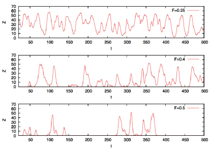
Figure 23: Numerical simulations performed with $\mu=1$ for $(7/16)L<x<(9/16)L$ and $\mu=-1/15.$ elsewhere for all $x$. We plot the total number of microorganisms $Z(t)$ for three different values of $F$, namely $F=0.25$ (upper panel), $F=0.4$ (middle panel) and $F=0.5$ (lower panel).

So far we have discussed the case of $\mu$ constant and positive. In some applications (both in biology and in physics) one may be interested to discuss $\mu$ with some non trivial space dependence. An interesting case, generalizing the work in [6], [7] and [12] is provided by the equation,

$$\partial_{t}c+\partial_{x}(Uc)=D\partial_{x}^{2}c+\mu(x)c-bc^{2},$$ (25)

with a turbulent convecting velocity field $U(x,t)=u_{0}+u(x,t)$ and where $\mu$ is positive on a small fraction of the whole domain and negative elsewhere. In this case, referred to as the ”oasis”, one would like to determine when $\langle c(x,t)\rangle$ can be significantly different from zero, i.e. when do the populations on an island or oasis survive when buffeted by the turbulent flows engendered by , say, a major storm (see [8] for a treatment of space-independent random convection). A qualitative prediction for $\langle c(x,t)\rangle$ results from the following argument: the extended and/or localization behaviour of $c$ depends on the ratio defined in Eq. (12). For small $\Gamma$ (i.e. small $F$) the solution must be extended and therefore one can predict that $c$ is significantly different from zero everywhere, wherever $\mu>0$. On the other hand, for large $\Gamma$, $c$ becomes localized. The probability for $c$ to be localized in one point or another is uniform on the whole domain. Thus, if the region where $\mu>0$ is significantly smaller then the region where $\mu<0$, $c$ should approach to zero for long enough time.

In Fig. (23), we show a numerical simulation performed for a oasis centered on $x=L/2$, performed with $\mu=1$ for $(7/16)L<x<(9/16)L$ and $\mu=-1/15.$ elsewhere for all $x$. Thus the spatial average of the growth rate is $L^{-1}\int_{0}^{L}dx\mu(x)=1/15.$. As a measure of $c$, we plot its spatial integral $Z(t)$ as a function of time. The numerical simulations have been done with $D=0.005$, $N=512$ and $u_{0}=0$. In Fig.(23) we show three different values of $F$. Let us recall that, when $\mu=1$ everywhere, as is now the case for the oasis, for $F\geq 0.25$, the system exhibits a transition from extended states to localized states, as illustrated in Fig. (15). As one can see, for $F\geq 0.4$ the population tends to crash as predicted by our simple arguments. It is however interesting to observe that the dynamics of $c$ is not at all trivial. For $F=0.4$ and $F=0.5$, $c$ seems to almost die and then recovers. Of course, our continuum equations neglect the discreteness of the population. At very low populations densities, a reference volume can contain a fractional number of organisms and extintion events are artificially supressed. Fig. (23) neverthelesst suggests an interesting feature of Eq. (25) with space dependent $\mu$, worth investigating in the future.

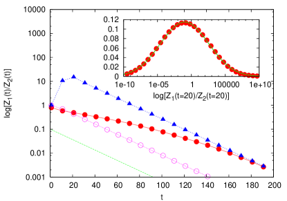
Figure 24: Numerical simulation of equations (26),(27) with $\mu_{1}=1.$ and $\mu_{2}=1.05$. We show the quantities $Z_{1}/Z_{2}$ (open circles) for the case with no turbulence. Note that $Z_{1}/Z_{2}$ decays to zero as $exp(-(\mu_{2}-\mu_{1})t)$ (green line) . When turbulence is acting, the dynamics becomes more intermitent as shown by the behavior of $\langle Z_{1}\rangle/\langle Z_{2}\rangle$ (close red circles) and and $\langle Z_{1}/Z_{2}\rangle$ (solid triangles). The symbol $\langle...\rangle$ means averaging over ensemble. In the insert, we show the probabiltiy distribution of $log[Z_{1}(t)/Z_{2}(t)]$, at $t=20$, which is well fitted by a guassian behavior.

Another interesting question tjhat deserves more detailed studies is the case two competing species with densities $c_{1}(x,t)$ and $c_{2}(x,t)$. To illustrate the problem, consider the coupled equations:

$$\partial_{t}c_{1}+\partial_{x}(Uc_{1})=D\partial_{x}^{2}c_{1}+\mu_{1}c_{1}(1-c_{1})-\mu_{2}c_{1}c_{2}$$ (26)

$$\partial_{t}c_{2}+\partial_{x}(Uc_{2})=D\partial_{x}^{2}c_{2}+\mu_{2}c_{2}(1-c_{2})-\mu_{1}c_{1}c_{2}$$ (27)

where $\mu_{2}>\mu_{1}$ and $0<\delta\mu\equiv\mu_{2}-\mu_{1}\ll\mu_{1}$. In this simplified model, Eqs. (26) and (27) describe the dynamics of two populations in which a ”mutant” density $c_{2}$ can out compete a wild type density $c_{1}$. In particular, upon specializing to one dimension and denoting $c_{sum}(x,t)\equiv c_{1}(x,t)+c_{2}(x,t)$, from Eq.s (26,27) we obtain:

$$\partial_{t}c_{sum}+\partial_{x}(Uc_{sum})=D\partial_{x}^{2}c_{sum}+(1-c_{sum})(\mu_{1}c_{1}+\mu_{2}c_{2})$$ (28)

Eq. (28) shows that, for $U=0$, $c_{sum}=1$ is an invariant subset, i.e., if at $t=0$, $c_{sum}=1$, then $c_{sum}=1$ for any $t$. The system has two stationary solutions, namely $c_{1}=1$,$c_{2}=0$ which is unstable, and $c_{1}=0$,$c_{2}=1$ which is stable. For $U=0$, any initial conditions is attracted to the stable solution. It is easy to check that the asymptotic time dependences in this subspace are of $Z_{1}\sim exp(-\delta\mu t)$ and $Z_{2}\sim 1-exp(-\delta\mu t)$, where $Z_{i}\equiv\int dxc_{i}(x,t)$.

In Fig. (24) we show the result of two different numerical simulations of Eqs. (26,27) with $\mu_{1}=1$ and $\mu_{2}=1.05$. The solutions have been obtained by using periodic boundary conditions, $L=1$, $D=0.005$ and a numerical resolution of $512$ grid points. The open circles represent the behavior of $log(Z_{1}(t)/Z_{2}(t))$ for $U=0$. As predicted by our simple analysis, $Z_{1}/Z_{2}$ decays quite rapidly towards $0$ as $exp(-\delta\mu t)$ (dashed green line in Fig. (24) . Note that $\delta\mu=0.05$, corresponding to a characterstic time $1/\delta\mu\sim 20$.

For $U\neq 0$, however, the time behavior is quite different. In particular, we choose $u_{0}=0$ and allow convection by a strong turbulent field with $F=0.8$. In Fig. (24), the red circles refer to $log(\langle Z_{1}(t)\rangle/\langle Z_{2}(t)\rangle)$ while the blue triangles refer to $log(\langle Z_{1}(t)/(Z_{2}(t)\rangle$. The symbol $\langle...\rangle$ is the ensemble average over $100$ realizations of the turbulent field, with the same initial conditions

$$c_{1}(x,t=0)=1\ \ c_{2}(x,t=0)=0\ \ for\ \ \ \ 0<x<\frac{L}{2}$$ (29)

$$c_{1}(x,t=0)=0\ \ c_{2}(x,t=0)=1\ \ for\ \ \ \frac{L}{2}<x<L$$ (30)

While the asymptotic states are still the same as for the case $F=0$ (the stability of the stationary solutions does not change), the population $c_{1}$ decays on a time scale longer than the $F=0$ one (i.e. $1/\delta\mu$). The rather large difference between $\langle Z_{1}(t)\rangle/\langle Z_{2}(t)\rangle$ and $\langle Z_{1}(t)/Z_{2}(t)\rangle$ is due to strong fluctuations in the ensemble. To highlight these fluctuations, we show in the insert of Fig. (24) the probability distribution $P(R)$ of the logarithmic ratio $R(t)\equiv log(Z_{1}(t)/Z_{2}(t))$ computed at $t=20$, which is well fitted by a gaussian distribution with a rather large variance. This implies that the ratio $Z_{1}/Z_{2}$ is a strongly intermittent quantity. To explain such a strong intremittency, note that the initial time behavior of the system strongly depends whether one of the two populations is spatially extended while the other sharply peaked. When the population $c_{1}(x,t)$ is extended while $c_{2}(x,t)$ is sharply peaked, the ratio $Z_{1}/Z_{2}$ becomes initially quite large. On the other hand, when $c_{2}(x,t)$ is extended and $c_{1}(x,t)$ sharply peaked, $Z_{1}/Z_{2}$ is very small. For long enough times, the two populations become correlated in space (by clustering and competing at the same accumulation points of $u(x,t)$) and the ratio $Z_{1}/Z_{2}$ eventually decays according to the expected behavior $exp(-\delta\mu t)$. Note that the characteristic turbulent mixing times in our simulations are much longer that the characteristic doubling times of the microorganisms, $\sim 1/\mu_{1}$ and $\sim 1/\mu_{2}$. This is the opposite of the situation in many microbiology laboratories, where organisms in test tubes are routinely mixed at a rapid rate overnight at Reynolds numbers of the order $10^{3}$. The situation studied here can, however, arise for microorganisms subject to turbulence in the ocean.

We close with comments on generalization to more that one dimension. When ”turbulent velocity field” $\vec{u}(x,.t)$ can be represented as $\nabla\Psi(x,t)$, with a suitable $\Psi$, most of the results discussed in this paper should be valid. However, in a real turbulent flow in higher dimensions, whether compressible or incompressible, the velocity field is not irrotational. For a real turbulent flow, we believe the localization discussed here will be reflected in a reduction of the space dimensions in the support of $c(\vec{x},t)$. For instance, in two dimension, we expect that $c(\vec{x},t)$ will become large on a one-dimensional filament while in three dimension $c(\vec{x},t)$ localizes on a two dimensional surface. For a review of related effects for biological organisms in oceanic flows at moderate Reynolds numbers see [17]

Following the multifractal language, there may be a full spectrum of dimensions which may characterize the statistical properties of localized states. It remains to be seen whether a sharp crossover (or an actual phase transition) similar to what has been shown in Secs. $3$ and $4$, will be observed in more than one dimension.

References

- [1] J.J. Wakika et. al. J. Physical Society of Japan, 63, 1205, (1994)
- [2] R. A. Fisher , The wave of advance of advantageous genes , Ann Eugenics, 7 (1937), 335.
- [3] J. A. Shapiro, J., and M. Dworkin. 1997. Bacteria as Multicellular Organisms. Oxford University Press, New York.
- [4] M. Matsushita, J. Wakita, H. Itoh, I. Rafols, T. Matsuyama, H. Sakaguchi, and M. Mimura. 1998. Interface growth and pattern formation in bacterial colonies. Physica A. 249, 517.
- [5] E. Ben-Jacob, O. Shochet, A. Tenebaum, I. Cohen, A. Czirok, and T. Vicsek. 1994. Genetic modeling of cooperative growth patterns in bacterial colonies. Nature. 368, 46.
- [6] D. R. Nelson, and N. M. Shnerb. 1998. Non-hermitian localization and population biology. Phys. Rev. E. 58:1383.
- [7] K.A. Dahmen, D. R. Nelson, and N. M. Shnerb. 2000. Life and death near a windy oasis. J. Math. Biol. 41:1-23.
- [8] T. Fransch and D.R. Nelson, J. Stat. Phys., 99, 1021, 2000.
- [9] J. Bec, 2003, Fractal clustering of inertial particles in random flows. Physical of Fluids, 15, L81. J. Bec, 2005, Multifractal concentrations of inertial particles in smooth random flows. Journal of Fluid Mechanics, 528, 255.
- [10] A. Kolmogorov, I. Petrovsky, and N. Piscounoff, Moscow Univ. Bull. Math. 1, 1 - 1937.
- [11] U. Frisch, Turbulence: The legacy of A.N. Kolmogorov (Cambridge University Press, Cambridge, 1995).
- [12] N. M. Shnerb, 2001, Extinction of a bacterial colony under forced convection in pie geometry. Phys. Rev. E 63:011906, and references therein.
- [13] T. Neicu, A. Pradhan, D. A. Larochelle, and A. Kudrolli. 2000. Extinction transition in bacterial colonies under forced convection. Phys. Rev. E. 62:1059 - 1062.
- [14] O. Hallatschek and D. R. Nelson, Theor. Popul. Biology, 73,1, 158, 2007.
- [15] L. Biferale, Annu., 2003, Rev. Fluid Mech. 35, 441.
- [16] Anderson P W 1958 Phys. Rev., 109, 1492
- [17] T. Tel et. al., Chemical and Biological Activity in Open Flows: A Dynamical Systems Approach, Phys. Reports, 413, 91, 2005