Iterated filtering

Abstract

Inference for partially observed Markov process models has been a longstanding methodological challenge with many scientific and engineering applications. Iterated filtering algorithms maximize the likelihood function for partially observed Markov process models by solving a recursive sequence of filtering problems. We present new theoretical results pertaining to the convergence of iterated filtering algorithms implemented via sequential Monte Carlo filters. This theory complements the growing body of empirical evidence that iterated filtering algorithms provide an effective inference strategy for scientific models of nonlinear dynamic systems. The first step in our theory involves studying a new recursive approach for maximizing the likelihood function of a latent variable model, when this likelihood is evaluated via importance sampling. This leads to the consideration of an iterated importance sampling algorithm which serves as a simple special case of iterated filtering, and may have applicability in its own right.

abstractwidth280pt

, , and TT1Supported by NSF Grants DMS-08-05533 and EF-04-30120, the Graham Environmental Sustainability Institute, the RAPIDD program of the Science & Technology Directorate, Department of Homeland Security, and the Fogarty International Center, National Institutes of Health.

[]This work was conducted as part of the Inference for Mechanistic Models Working Group supported by the National Center for Ecological Analysis and Synthesis, a Center funded by NSF Grant DEB-0553768, the University of California, Santa Barbara and the State of California.

keywordAMSMSC2010 subject classification.

1 Introduction

Partially observed Markov process (POMP) models are of widespread importance throughout science and engineering. As such, they have been studied under various names including state space models [Durbin and Koopman (2001)], dynamic models [West and Harrison (1997)] and hidden Markov models [Cappé, Moulines and Rydén (2005)]. Applications include ecology [Newman et al. (2009)], economics [Fernández-Villaverde and Rubio-Ramírez (2007)], epidemiology [King et al. (2008)], finance [Johannes, Polson and Stroud (2009)], meteorology [Anderson and Collins (2007)], neuroscience [Ergün et al. (2007)] and target tracking [Godsill et al. (2007)].

This article investigates convergence of a Monte Carlo technique for estimating unknown parameters of POMPs, called iterated filtering, which was proposed by Ionides, Bretó and King (2006). Iterated filtering algorithms repeatedly carry out a filtering procedure to explore the likelihood surface at increasingly local scales in search of a maximum of the likelihood function. In several case-studies, iterated filtering algorithms have been shown capable of addressing scientific challenges in the study of infectious disease transmission, by making likelihood-based inference computationally feasible in situations where this was previously not the case [King et al. (2008); Bretó et al. (2009); He, Ionides and King (2010); Laneri et al. (2010)]. The partially observed nonlinear stochastic systems arising in the study of disease transmission and related ecological systems are a challenging environment to test statistical methodology [Bjørnstad and Grenfell (2001)], and many statistical methodologies have been tested on these systems in the past fifty years [e.g., Cauchemez and Ferguson (2008); Toni et al. (2008); Keeling and Ross (2008); Ferrari et al. (2008); Morton and Finkenstädt (2005); Grenfell, Bjornstad and Finkenstädt (2002); Kendall et al. (1999); Bartlett (1960); Bailey (1955)]. Since iterated filtering has already demonstrated potential for generating state-of-the-art analyses on a major class of scientific models, we are motivated to study its theoretical justification. The previous theoretical investigation of iterated filtering, presented by Ionides, Bretó and King (2006), did not engage directly in the Monte Carlo issues relating to practical implementation of the methodology. It is relatively easy to check numerically that a maximum has been attained, up to an acceptable level of Monte Carlo uncertainty, and therefore one can view the theory of Ionides, Bretó and King (2006) as motivation for an algorithm whose capabilities were proven by demonstration. However, the complete framework presented in this article gives additional insights into the potential capabilities, limitations and generalizations of iterated filtering.

The foundation of our iterated filtering theory is a Taylor series argument which we present first in the case of a general latent variable model in Section 2. This leads us to propose and analyze a novel iterated importance sampling algorithm for maximizing the likelihood function of latent variable models. Our motivation is to demonstrate a relatively simple theoretical result which is then extended to POMP models in Section 3. However, this result also demonstrates the broader possibilities of the underlying methodological approach.

The iterated filtering and iterated importance sampling algorithms that we study have an attractive practical property that the model for the unobserved process enters the algorithm only through the requirement that realizations can be generated at arbitrary parameter values. This property has been called plug-and-play [Bretó et al. (2009); He, Ionides and King (2010)] since it permits simulation code to be simply plugged into the inference procedure. A concept closely related to plug-and-play is that of implicit models for which the model is specified via an algorithm to generate stochastic realizations [Diggle and Gratton (1984); Bretó et al. (2009)]. In particular, evaluation of the likelihood function for implicit models is considered unavailable. Implicit models arise when the model is represented by a “black box” computer program. A scientist investigates such a model by inputting parameter values, receiving as output from the “black box” independent draws from a stochastic process, and comparing these draws to the data to make inferences. For an implicit model, only plug-and-play statistical methodology can be employed. Other plug-and-play methods proposed for partially observed Markov models include approximate Bayesian computations implemented via sequential Monte Carlo [Liu and West (2001); Toni et al. (2008)], an asymptotically exact Bayesian technique combining sequential Monte Carlo with Markov chain Monte Carlo [Andrieu, Doucet and Holenstein (2010)], simulation-based forecasting [Kendall et al. (1999)], and simulation-based spectral analysis [Reuman et al. (2006)]. Further discussion of the plug-and-play property is included in the discussion of Section 4.

2 Iterated importance sampling

Let $f_{XY}(x,y;\theta)$ be the joint density of a pair of random variables $(X,Y)$ depending on a parameter $\theta\in\mathbb{R}^{p}$. We suppose that $(X,Y)$ takes values in some measurable space ${\mathfrak{X}}\times{\mathfrak{Y}}$, and $f_{XY}(x,y;\theta)$ is defined with respect to some $\sigma$-finite product measure which we denote by $dx\,dy$. We suppose that the observed data consist of a fixed value $y^{*}\in{\mathfrak{Y}}$, with $X$ being unobserved. Therefore, $\{f_{XY}(x,y;\theta),\theta\in\mathbb{R}^{p}\}$ defines a general latent variable statistical model. We write the marginal densities of $X$ and $Y$ as $f_{X}(x;\theta)$ and $f_{Y}(y;\theta)$, respectively. The measurement model is the conditional density of the observed variable given the latent variable $X$, written as $f_{Y|X}(y\mid x;\theta)$. The log likelihood function is defined as $\ell(\theta)=\log f_{Y}(y^{*};\theta)$. We consider the problem of calculating the maximum likelihood estimate, defined as $\hat{\theta}=\arg\max_{\theta}\ell(\theta)$.

We consider an iterated importance sampling algorithm which gives a plug-and-play approach to likelihood based inference for implicit latent variable models, based on generating simulations at parameter values in a neighborhood of the current parameter estimate to refine this estimate. This shares broadly similar goals with other Monte Carlo methods proposed for latent variable models [e.g., Johansen, Doucet and Davy (2008); Qian and Shapiro (2006)], and in a more general context has similarities with evolutionary optimization strategies [Beyer (2001)]. We emphasize that the present motivation for proposing and studying iterated importance sampling is to lay the groundwork for the results on iterated filtering in Section 3. However, the successes of iterated filtering methodology on POMP models also raise the possibility that related techniques may be useful in other latent variable situations.

We define the stochastically perturbed model to be a triplet of random variables $(\breve{X},\breve{Y},\breve{\Theta})$, with perturbation parameter $\tau$ and parameter $\theta$, having a joint density on ${\mathfrak{X}}\times{\mathfrak{Y}}\times\mathbb{R}^{p}$ specified as

$$g_{\breve{X},\breve{Y},\breve{\Theta}}(x,y,\breve{\vartheta};\theta,\tau)=f_{XY}(x,y;\breve{\vartheta})\tau^{-p}\kappa_{\tau}\bigl{(}(\breve{\vartheta}-\theta)/\tau\bigr{)}.$$ (1)

Here, $\{\kappa_{\tau},\tau>0\}$ is a collection of mean-zero densities on $\mathbb{R}^{p}$ (with respect to Lebesgue measure) satisfying condition (A1) below:

For each $\tau>0$, $\kappa_{\tau}$ is supported on a compact set $K_{0}\subset\mathbb{R}^{p}$ independent of $\tau$. Condition (A1) can be satisfied by the arbitrary selection of $\kappa_{\tau}$. At first reading, one can imagine that $\kappa_{\tau}$ is fixed, independent of $\tau$. However, the additional generality will be required in Section 3.

We start by showing a relationship between conditional moments of $\breve{\Theta}$ and the derivative of the log likelihood function, in Theorem 1. We write ${\breve{\mathbb{E}}_{\theta,\tau}}[\cdot]$ to denote expectation with respect to the stochastically perturbed model. We write $u\in\mathbb{R}^{p}$ to specify a column vector, with $u^{\prime}$ being the transpose of $u$. For a function $f=(f_{1},\ldots,f_{m})^{\prime}\dvtx\mathbb{R}^{p}\to\mathbb{R}^{m}$, we write $\int f(u)\,du$ for the vector $(\int f_{1}(u)\,du,\ldots,\int f_{m}(u)\,du)^{\prime}\in\mathbb{R}^{m}$; For any function $f\dvtx\mathbb{R}^{p}\to\mathbb{R}$, we write $\nabla f(u)$ to denote the column vector gradient of $f$, with $\nabla^{2}f(u)$ being the second derivative matrix. We write $|\cdot|$ for the absolute value of a vector or the largest absolute eigenvalue of a square matrix. We write $B(r)=\{u\in\mathbb{R}^{p}\dvtx|u|\leq r\}$ for the ball of radius $r$ in $\mathbb{R}^{p}$. We assume the following regularity condition:

ℓ(θ) is twice differentiable. For any compact set ${K_{1}}\subset\mathbb{R}^{p}$,

$$\sup_{\theta\in{K_{1}}}|\nabla\ell(\theta)|<\infty\quad\mbox{and}\quad\sup_{\theta\in{K_{1}}}|\nabla^{2}\ell(\theta)|<\infty.$$

Theorem 1

Assume conditions (A1), (A2). Let $h\dvtx\mathbb{R}^{p}\to\mathbb{R}^{m}$ be a measurable function possessing constants $\alpha\geq 0$, $c>0$ and $\varepsilon>0$ such that, whenever $u\in B(\varepsilon)$,

$$|h(u)|\leq c|u|^{\alpha}.$$ (2)

Define $\tau_{0}=\sup\{\tau\dvtx K_{0}\subset B(\varepsilon/\tau)\}$. For any compact set ${K_{2}}\subset\mathbb{R}^{p}$ there exists ${C_{1}}<\infty$ and a positive constant $\tau_{1}\leq\tau_{0}$ such that, for all $0<\tau\leq\tau_{1}$,

$$\sup_{\theta\in{K_{2}}}\biggl{|}{\breve{\mathbb{E}}_{\theta,\tau}}[h(\breve{\Theta}-\theta)\mid\breve{Y}=y^{*}]-\int h(\tau u)\kappa_{\tau}(u)\,du$$

$$\hskip 76.0pt{}-\tau\biggl{\{}\int h(\tau u)u^{\prime}\kappa_{\tau}(u)\,du\biggr{\}}\nabla\ell(\theta)\biggr{|}$$ (3)

$$\qquad\leq{C_{1}}\tau^{2+\alpha}.$$

Let $g_{\breve{Y}|\breve{\Theta}}(y\mid\breve{\vartheta};\theta,\tau)$ denote the conditional density of $\breve{Y}$ given $\breve{\Theta}$. We note that $g_{\breve{Y}|\breve{\Theta}}$ does not depend on either $\tau$ or $\theta$, and so we omit these dependencies below. Then, $g_{\breve{Y}|\breve{\Theta}}(y^{*}\mid\breve{\vartheta})=\int f_{XY}(x,y^{*};\breve{\vartheta})\,dx=\exp(\ell(\breve{\vartheta}))$. Changing variable to $u=(\breve{\vartheta}-\theta)/\tau$, we calculate

$${\breve{\mathbb{E}}_{\theta,\tau}}[h(\breve{\Theta}-\theta)\mid\breve{Y}=y^{*}] = \frac{\int h(\breve{\vartheta}-\theta)g_{\breve{Y}|\breve{\Theta}}(y^{*}\mid\breve{\vartheta})\tau^{-p}\kappa_{\tau}((\breve{\vartheta}-\theta)\big{/}\tau)\,d\breve{\vartheta}}{\int g_{\breve{Y}|\breve{\Theta}}(y^{*}\mid\breve{\vartheta})\tau^{-p}\kappa_{\tau}((\breve{\vartheta}-\theta)\big{/}\tau)\,d\breve{\vartheta}}$$

$$= \frac{\int h(\tau u)\exp\{\ell(\theta+\tau u)-\ell(\theta)\}\kappa_{\tau}(u)\,du}{\int\exp\{\ell(\theta+\tau u)-\ell(\theta)\}\kappa_{\tau}(u)\,du}.$$

Applying the Taylor expansion $e^{x}=1+x+(\int_{0}^{1}(1-t)e^{tx}\,dt)x^{2}$ to the numerator of (2) gives

$$\int\exp\{\ell(\theta+\tau u)-\ell(\theta)\}h(\tau u)\kappa_{\tau}(u)\,du$$

$$\qquad=\int h(\tau u)\kappa_{\tau}(u)\,du+\int\{\ell(\theta+\tau u)-\ell(\theta)\}h(\tau u)\kappa_{\tau}(u)\,du$$ (5)

$$\qquad\quad{}+\int\biggl{(}\int_{0}^{1}(1-t)e^{t(\ell(\theta+\tau u)-\ell(\theta))}\,dt\biggr{)}\{\ell(\theta+\tau u)-\ell(\theta)\}^{2}h(\tau u)\kappa_{\tau}(u)\,du.$$

We now expand the second term on the right-hand side of (2) by making use of the Taylor expansion

$$\ell(\theta+\tau u)-\ell(\theta) = \tau u^{\prime}\int_{0}^{1}\nabla\ell(\theta+t\tau u)\,dt$$

$$= \tau u^{\prime}\nabla\ell(\theta)+\tau u^{\prime}\int_{0}^{1}\{\nabla\ell(\theta+t\tau u)-\nabla\ell(\theta)\}\,dt$$

and defining $\psi_{\tau,h}(\theta)=\int h(\tau u)\kappa_{\tau}(u)\,du+\tau\{\int h(\tau u)u^{\prime}\kappa_{\tau}(u)\,du\}\nabla\ell(\theta)$. This allows us to rewrite (2) as

$$\int\exp\{\ell(\theta+\tau u)-\ell(\theta)\}h(\tau u)\kappa_{\tau}(u)\,du=\psi_{\tau,h}(\theta)+{R_{1}}(\theta,\tau),$$ (7)

where

$${R_{1}}(\theta,\tau)$$

$$\qquad=\tau\int h(\tau u)u^{\prime}\biggl{(}\int_{0}^{1}\{\nabla\ell(\theta+t\tau u)-\nabla\ell(\theta)\}\,dt\biggr{)}\kappa_{\tau}(u)\,du$$

$$\qquad\quad{}+\int\biggl{(}\int_{0}^{1}(1-t)e^{t(\ell(\theta+\tau u)-\ell(\theta))}\,dt\biggr{)}\{\ell(\theta+\tau u)-\ell(\theta)\}^{2}h(\tau u)\kappa_{\tau}(u)\,du.$$

As a consequence of (A2), we have

$$\sup_{\theta\in{K_{2}}}\sup_{u\in K_{0}}\sup_{t\in[0,\tau_{0}]}\bigl{(}|\nabla\ell(\theta+tu)|+|\nabla^{2}\ell(\theta+tu)|\bigr{)}<\infty.$$ (8)

Combining (8) with the assumption that $K_{0}\subset B(\varepsilon/\tau)$, we deduce the existence of a finite constant ${C_{2}}$ such that

$$\sup_{\theta\in{K_{2}}}|{R_{1}}(\theta,\tau)|\leq{C_{2}}\tau^{2+\alpha}.$$ (9)

We bound the denominator of (2) by considering the special case of (7) in which $h$ is taken to be the unit function, $h(u)=1$. Noting that $\int u\kappa_{\tau}(u)\,du=0$, we see that $\psi_{\tau,1}(\theta)=1$ and so (7) yields

$$\int\exp\{\ell(\theta+\tau u)-\ell(\theta)\}\kappa_{\tau}(u)\,du=1+{R_{2}}(\theta,\tau)$$

with ${R_{2}}(\theta,\tau)$ having a bound

$$\sup_{\theta\in{K_{2}}}|{R_{2}}(\theta,\tau)|\leq{C_{3}}\tau^{2}$$ (10)

for some finite constant ${C_{3}}$. We now note the existence of a finite constant ${C_{4}}$ such that

$$\sup_{\theta\in{K_{2}}}|\psi_{\tau,h}(\theta)|\leq{C_{4}}\tau^{\alpha}$$ (11)

implied by (2), (A1) and (A2). Combining (9), (10) and (11) with the identity

$${\breve{\mathbb{E}}_{\theta,\tau}}\bigl{(}h(\breve{\Theta}-\theta)\mid\breve{Y}=y^{*}\bigr{)}-\psi_{\tau,h}(\theta)=\frac{{R_{1}}(\theta,\tau)-{R_{2}}(\theta,\tau)\psi_{\tau,h}(\theta)}{1+{R_{2}}(\theta,\tau)},$$

and requiring $\tau_{1}<(2{C_{3}})^{-1/2}$, we obtain that

$$\sup_{\theta\in{K_{2}}}\bigl{|}{\breve{\mathbb{E}}_{\theta,\tau}}\bigl{(}h(\breve{\Theta}-\theta)\mid\breve{Y}=y^{*}\bigr{)}-\psi_{\tau,h}(\theta)\bigr{|}\leq{C_{5}}\tau^{2+\alpha}$$ (12)

for some finite constant ${C_{5}}$. Substituting the definition of $\psi_{\tau,h}(\theta)$ into (12) gives (1) and hence completes the proof.

One natural choice is to take $h(u)=u$ in Theorem 1. Supposing that $\kappa_{\tau}$ has associated positive definite covariance matrix $\breve{\Sigma}$, independent of $\tau$, this leads to an approximation to the derivative of the log likelihood given by

$$\bigl{|}\nabla\ell(\theta)-\{(\tau^{2}\breve{\Sigma})^{-1}({\breve{\mathbb{E}}_{\theta,\tau}}[\breve{\Theta}\mid\breve{Y}=y^{*}]-\theta)\}\bigr{|}\leq{C_{6}}\tau$$ (13)

for some finite constant ${C_{6}}$, with the bound being uniform over $\theta$ in any compact subset of $\mathbb{R}^{p}$. The quantity ${\breve{\mathbb{E}}_{\theta,\tau}}[\breve{\Theta}\mid\breve{Y}=y^{*}]$ does not usually have a closed form, but a plug-and-play Monte Carlo estimate of it is available by importance sampling, supposing that one can draw from $f_{X}(x;\theta)$ and evaluate $f_{Y|X}(y^{*}\mid x;\theta)$. Numerical approximation of moments is generally more convenient than approximating derivatives, and this is the reason that the relationship in (13) may be useful in practice. However, one might suspect that there is no “free lunch” and therefore the numerical calculation of the left-hand side of (13) should become fragile as $\tau$ becomes small. We will see that this is indeed the case, but that iterated importance sampling methods mitigate the difficulty to some extent by averaging numerical error over subsequent iterations.

Input:

• Latent variable model described by a latent variable density $f_{X}(x;\theta)$, measurement model $f_{Y|X}(y\mid x;\theta)$, and data $y^{*}$.

• Perturbation density $\kappa$ having compact support, zero mean and positive definite covariance matrix $\breve{\Sigma}$.

• Positive sequences $\{\tau_{m}\}$ and $\{a_{m}\}$

• Integer sequence of Monte Carlo sample sizes, $\{J_{m}\}$

• Initial parameter estimate, $\hat{\theta}_{1}$

• Number of iterations, $M$

Procedure:

1. [3]

2. for $m$ in $1\dvtx M$

3. for $j$ in $1\dvtx J_{m}$

4. draw $Z_{j,m}\sim\kappa(\cdot)$ and set $\breve{\Theta}_{j,m}=\hat{\theta}_{m}+\tau_{m}Z_{j,m}$

5. draw $\breve{X}_{j,m}\sim f_{X}(\cdot;\breve{\Theta}_{j,m})$

6. set $w_{j}=f_{Y|X}(y^{*}\mid\breve{X}_{j,m};\breve{\Theta}_{j,m})$

7. end for

8. calculate $D_{m}=\tau_{m}^{-2}\breve{\Sigma}^{-1}\{(\sum_{j=1}^{J_{m}}w_{j})^{-1}(\sum_{j=1}^{J_{m}}w_{j}\breve{\Theta}_{j,m})-\hat{\theta}_{m}\}$

9. update estimate: $\hat{\theta}_{m+1}=\hat{\theta}_{m}+a_{m}D_{m}$

10. end for

Output:

• parameter estimate $\hat{\theta}_{M+1}$

Algorithm 1 A basic iterated importance sampling procedure. The Monte Carlo random variables required at each iteration are presumed to be drawn independently. Theorem 2 gives sufficient conditions for $\hat{\theta}_{M}$ to converge to the maximum likelihood estimate as $M\to\infty$.

A trade-off between bias and variance is to be expected in any Monte Carlo numerical derivative, a classic example being the Kiefer–Wolfowitz algorithm [Kiefer and Wolfowitz (1952); Spall (2003)]. Algorithms which are designed to balance such trade-offs have been extensively studied under the label of stochastic approximation [Kushner and Yin (2003); Spall (2003); Andrieu, Moulines and Priouret (2005)]. Algorithm 1 is an example of a basic stochastic approximation algorithm taking advantage of (13). As an alternative, the derivative approximation in (13) could be combined with a stochastic line search algorithm. In order to obtain the plug-and-play property, we consider an algorithm that draws from $f_{X}(x;\theta)$ for iteratively selected values of $\theta$. This differs from other proposed iterative importance sampling algorithms which aim to construct improved importance sampling distributions [e.g., Celeux, Marin and Robert (2006)]. In principle, a procedure similar to Algorithm 1 could take advantage of alternative choices of importance sampling distribution: the fundamental relationship in Theorem 1 is separate from the numerical issues of computing the required conditional expectation by importance sampling. Theorem 2 gives sufficient conditions for the convergence of Algorithm 1 to the maximum likelihood estimate. To control the variance of the importance sampling weights, we suppose:

For any compact set ${K_{3}}\subset\mathbb{R}^{p}$,

$$\sup_{\theta\in{K_{3}},x\in{\mathfrak{X}}}f_{Y|X}(y^{*}\mid x;\theta)<\infty.$$

We also adopt standard sufficient conditions for stochastic approximation methods: [(B2)]

Define $\zeta(t)$ to be a solution to $d\zeta/dt=\nabla\ell(\zeta(t))$. Suppose that $\hat{\theta}$ is an asymptotically stable equilibrium point, meaning that (i) for every $\eta>0$ there exists a $\delta(\eta)$ such that $|\zeta(t)-\hat{\theta}|\leq\eta$ for all $t>0$ whenever $|\zeta(0)-\hat{\theta}|\leq\delta$, and (ii) there exists a $\delta_{0}$ such that $\zeta(t)\to\hat{\theta}$ as $t\to\infty$ whenever $|\zeta(0)-\hat{\theta}|\leq\delta_{0}$.

With probability one, $\sup_{m}|\hat{\theta}_{m}|<\infty$. Further, $\hat{\theta}_{m}$ falls infinitely often into a compact subset of $\{\zeta(0)\dvtx\lim_{t\to\infty}\zeta(t)=\hat{\theta}\}$. Conditions (B1) and (B2) are the basis of the classic results of Kushner and Clark (1978). Although research into stochastic approximation theory has continued [e.g., Kushner and Yin (2003); Andrieu, Moulines and Priouret (2005); Maryak and Chin (2008)], (B1) and (B2) remain a textbook approach [Spall (2003)]. The relative simplicity and elegance of Kushner and Clark (1978) makes an appropriate foundation for investigating the links between iterated filtering, sequential Monte Carlo and stochastic approximation theory. There is, of course, scope for variations on our results based on the diversity of available stochastic approximation theorems. Although neither (B1) and (B2) nor alternative sufficient conditions are easy to verify, stochastic approximation methods have nevertheless been found effective in many situations. Condition (B2) is most readily satisfied if $\hat{\theta}_{m}$ is constrained to a neighborhood in which $\hat{\theta}$ is a unique local maximum, which gives a guarantee of local rather than global convergence. Global convergence results have been obtained for related stochastic approximation procedures [Maryak and Chin (2008)] but are beyond the scope of this current paper. The rate assumptions in Theorem 2 are satisfied, for example, by $a_{m}=m^{-1}$, $\tau_{m}^{2}=m^{-1}$ and $J_{m}=m^{(\delta+1/2)}$ for $\delta>0$.

Theorem 2

Let $\{a_{m}\}$, $\{\tau_{m}\}$ and $\{J_{m}\}$ be positive sequences with $\tau_{m}\to 0$, $J_{m}\tau_{m}\to\infty$, $a_{m}\to 0$, $\sum_{m}a_{m}=\infty$ and $\sum_{m}a_{m}^{2}J_{m}^{-1}\tau_{m}^{-2}<\infty$. Let $\hat{\theta}_{m}$ be defined via Algorithm 1. Assuming (A1)–(A3) and (B1) and (B2),$\lim_{m\to\infty}\hat{\theta}_{m}=\hat{\theta}$ with probability one.

The quantity $D_{m}$ in line 7 of Algorithm 1 is a self-normalized Monte Carlo importance sampling estimate of

$$(\tau_{m}^{2}\breve{\Sigma})^{-1}\{{\mathbb{E}}_{\hat{\theta}_{m},\tau_{m}}[\breve{\Theta}\mid\breve{Y}=y^{*}]-\hat{\theta}_{m}\}.$$

We can therefore apply Corollary 8 from Section .2, writing $E_{\mathit{MC}}$ and $\operatorname{Var}_{\mathit{MC}}$ for the Monte Carlo expectation and variance resulting from carrying out Algorithm 1 conditional on the data $y^{*}$. This gives

$$\bigl{|}E_{\mathit{MC}}\bigl{[}D_{m}-(\tau_{m}^{2}\breve{\Sigma})^{-1}\{{\mathbb{E}}_{\hat{\theta}_{m},\tau_{m}}[\breve{\Theta}\mid\breve{Y}=y^{*}]-\hat{\theta}_{m}\}\bigr{]}\bigr{|}$$

(14)

$$\qquad\leq\frac{{C_{7}}(\sup_{x\in{\mathfrak{X}}}f_{Y|X}(y^{*}\mid x;\hat{\theta}_{m}))^{2}}{\tau_{m}J_{m}(f_{Y}(y^{*};\hat{\theta}_{m}))^{2}},$$

$$|\operatorname{Var}_{\mathit{MC}}(D_{m})|\leq\frac{{C_{8}}(\sup_{x\in{\mathfrak{X}}}f_{Y|X}(y^{*}\mid x;\hat{\theta}_{m}))^{2}}{\tau_{m}^{2}J_{m}(f_{Y}(y^{*};\hat{\theta}_{m}))^{2}}$$ (15)

for finite constants ${C_{7}}$ and ${C_{8}}$ which do not depend on $J$, $\hat{\theta}_{m}$ or $\tau_{m}$. Having assumed the conditions for Theorem 1, we see from (13) and (2) that $D_{m}$ provides an asymptotically unbiased Monte Carlo estimate of $\nabla\ell(\hat{\theta}_{m})$ in the sense of (B5) of Theorem 6 in Section .1. In addition, (15) justifies (B4) of Theorem 6. The remaining conditions of Theorem 6 hold by hypothesis.

3 Iterated filtering for POMP models

Let $\{X(t),t\in T\}$ be a Markov process [Rogers and Williams (1994)] with $X(t)$ taking values in a measurable space ${\mathfrak{X}}$. The time index set $T\subset\mathbb{R}$ may be an interval or a discrete set, but we are primarily concerned with a finite subset of times $t_{1}<t_{2}<\cdots<t_{N}$ at which $X(t)$ is observed, together with some initial time $t_{0}<t_{1}$. We write $X_{0\dvtx N}=(X_{0},\ldots,X_{N})=(X(t_{0}),\ldots,X(t_{N}))$. We write $Y_{1\dvtx N}=(Y_{1},\ldots,Y_{N})$ for a sequence of random variables taking values in a measurable space ${\mathfrak{Y}}^{N}$. We assume that $X_{0\dvtx N}$ and $Y_{1\dvtx N}$ have a joint density $f_{X_{0\dvtx N},Y_{1\dvtx N}}(x_{0\dvtx n},y_{1\dvtx n};\theta)$ on ${\mathfrak{X}}^{N+1}\times{\mathfrak{Y}}^{N}$, with $\theta$ being an unknown parameter in $\mathbb{R}^{p}$. A POMP model may then be specified by an initial density $f_{X_{0}}(x_{0};\theta)$, conditional transition densities $f_{X_{n}|X_{n-1}}(x_{n}\mid x_{n-1};\theta)$ for $1\leq n\leq N$, and the conditional densities of the observation process which are assumed to have the form $f_{Y_{n}|Y_{1\dvtx n-1},X_{0\dvtx n}}(y_{n}\mid y_{1\dvtx n-1},x_{0\dvtx n};\theta)=f_{Y_{n}|X_{n}}(y_{n}\mid x_{n};\theta)$. We use subscripts of $f$ to denote the required joint and conditional densities. We write $f$ without subscripts to denote the full collection of densities and conditional densities, and we call such an $f$ the generic density of a POMP model. The data are a sequence of observations by $y^{*}_{1\dvtx N}=(y^{*}_{1},\ldots,y^{*}_{N})\in{\mathfrak{Y}}^{N}$, considered as fixed. We write the log likelihood function of the data for the POMP model as $\ell_{N}(\theta)$ where

$$\ell_{n}(\theta)=\log\int f_{X_{0}}(x_{0};\theta)\prod_{k=1}^{n}f_{X_{k},Y_{k}|X_{k-1}}(x_{k},y^{*}_{k}\mid x_{k-1};\theta)\,dx_{0\dvtx n}$$

for $1\leq n\leq N$. Our goal is to find the maximum likelihood estimate, $\hat{\theta}=\arg\max_{\vartheta}\ell_{N}(\theta)$.

It will be helpful to construct a POMP model $\bar{f}$ which expands the model $f$ by allowing the parameter values to change deterministically at each time point. Specifically, we define a sequence $\vartheta_{0\dvtx N}=(\vartheta_{0},\ldots,\vartheta_{N})\in\{\mathbb{R}^{p}\}^{N+1}$. We then write $(\overline{X}_{0\dvtx N},\overline{Y}_{1\dvtx N})\in{\mathfrak{X}}^{N+1}\times{\mathfrak{Y}}^{N}$ for a POMP with generic density $\overline{f}$ specified by the joint density

$$\bar{f}_{\overline{X}_{0\dvtx N},\overline{Y}_{1\dvtx N}}(x_{0\dvtx N},y_{1\dvtx N};\vartheta_{0\dvtx n})$$

(16)

$$\qquad=f_{X_{0}}(x_{0};\vartheta_{0})\prod_{k=1}^{N}f_{Y_{k},X_{k}|X_{k-1}}(y_{k},x_{k}\mid x_{k-1};\vartheta_{k}).$$

We write the log likelihood of $y^{*}_{1\dvtx n}$ for the model $\overline{f}$ as $\overline{\ell}_{n}(\vartheta_{0\dvtx n})=\break\log\bar{f}_{\overline{Y}_{1\dvtx n}}(y^{*}_{1\dvtx n};\vartheta_{0\dvtx n})$. We write $\theta^{[k]}$ to denote $k$ copies of $\theta\in\mathbb{R}^{p}$, concatenated in a column vector, so that $\ell_{n}(\theta)=\overline{\ell}_{n}(\theta^{[n+1]})$. We write $\nabla_{i}\overline{\ell}_{n}(\vartheta_{0\dvtx n})$ for the partial derivative of $\overline{\ell}_{n}$ with respect to $\vartheta_{i}$, for $i=0,\ldots,n$. An application of the chain rule gives the identity

$$\nabla\ell_{n}(\theta)=\sum_{i=0}^{n}\nabla_{i}\overline{\ell}_{n}\bigl{(}\theta^{[n+1]}\bigr{)}.$$ (17)

The regularity condition employed for Theorem 3 below is written in terms of this deterministically perturbed model:

For each $1\leq n\leq N$, $\overline{\ell}_{n}(\theta_{0\dvtx n})$ is twice differentiable. For any compact subset $K$ of $\{\mathbb{R}^{p}\}^{n+1}$ and each $0\leq i\leq n$,

$$\sup_{\theta_{0\dvtx n}\in K}|\nabla_{i}\overline{\ell}_{n}(\theta_{0\dvtx n})|<\infty\quad\mbox{and}\quad\sup_{\theta_{0\dvtx n}\in K}|\nabla_{i}^{2}\overline{\ell}_{n}(\theta_{0\dvtx n})|<\infty.$$ (18)

Condition (A4) is a nonrestrictive smoothness assumption. However, the relationship between smoothness of the likelihood function, the transition density $f_{X_{k}|X_{k-1}}(x_{k}\mid x_{k-1};\theta)$, and the observation density $f_{Y_{k}|X_{k}}(y_{k}\mid x_{k};\theta)$ is simple to establish only under the restrictive condition that ${\mathfrak{X}}$ is a compact set. Therefore, we note an alternative to (A4) which is more restrictive but more readily checkable:

${\mathfrak{X}}$ is compact. Both $f_{X_{k}|X_{k-1}}(x_{k}\mid x_{k-1};\theta)$ and $f_{Y_{k}|X_{k}}(y_{k}\mid x_{k};\theta)$ are twice differentiable with respect to $\theta$. These derivatives are continuous with respect to $x_{k-1}$ and $x_{k}$.

Iterated filtering involves introducing an auxiliary POMP model in which a time-varying parameter process $\{\breve{\Theta}_{n},0\leq n\leq N\}$ is introduced. Let $\kappa$ be a probability density function on $\mathbb{R}^{p}$ having compact support, zero mean and covariance matrix $\Sigma$. Let $Z_{0},\ldots,Z_{N}$ be $N$ independent draws from $\kappa$. We introduce two perturbation parameters, $\sigma$ and $\tau$, and construct a process $\breve{\Theta}_{0\dvtx N}$ by setting $\breve{\Theta}_{0}=\vartheta_{0}+\tau Z_{0}$ and $\breve{\Theta}_{k}=\vartheta_{k}+\tau Z_{0}+\sigma\sum_{j=1}^{k}Z_{j}$ for $1\leq k\leq N$. The joint density of $\breve{\Theta}_{0\dvtx N}$ is written as $g_{\breve{\Theta}_{0\dvtx N}}(\breve{\vartheta}_{0\dvtx N};\vartheta_{0\dvtx N},\sigma,\tau)$. We define the stochastically perturbed POMP model $g$ with a Markov process $\{(\breve{X}_{n},\breve{\Theta}_{n}),0{\leq}n{\leq}N\}$, observation process $\breve{Y}_{1\dvtx N}$ and parameter $(\vartheta_{0\dvtx N},\sigma,\tau)$ by the joint density

$$g_{\breve{X}_{0\dvtx N},\breve{\Theta}_{0\dvtx N},\breve{Y}_{1\dvtx N}}(x_{0\dvtx N},\breve{\vartheta}_{0\dvtx N},y_{1\dvtx N};\vartheta_{0\dvtx N},\sigma,\tau)$$

$$\qquad=g_{\breve{\Theta}_{0\dvtx N}}(\breve{\vartheta}_{0\dvtx N};\vartheta_{0\dvtx N},\sigma,\tau)\bar{f}_{\overline{X}_{0\dvtx N},\overline{Y}_{1\dvtx N}}(x_{0\dvtx N},y_{1\dvtx N};\breve{\vartheta}_{0\dvtx N}).$$

We seek a result analogous to Theorem 1 which takes into account the specific structure of a POMP. Theorem 3 below gives a way to approximate $\nabla\ell_{N}(\theta)$ in terms of moments of the filtering distributions for $g$. We write ${\breve{\mathbb{E}}}_{\vartheta_{0\dvtx n},\sigma,\tau}$ and $\breve{\operatorname{Var}}_{\vartheta_{0\dvtx n},\sigma,\tau}$ for the expectation and variance, respectively, for the model $g$. We will be especially interested in the situation where $\vartheta_{0\dvtx n}=\theta^{[n+1]}$, which leads us to define the following filtering means and prediction variances:

$$\breve{\theta}^{F}_{n} = \breve{\theta}^{F}_{n}(\theta,\sigma,\tau)={\breve{\mathbb{E}}}_{\theta^{[n+1]},\sigma,\tau}[\breve{\Theta}_{n}\mid\breve{Y}_{1\dvtx n}=y^{*}_{1\dvtx n}]$$ (19)

$$= \int\breve{\vartheta}_{n}g_{\breve{\Theta}_{n}|\breve{Y}_{1\dvtx n}}\bigl{(}\breve{\vartheta}_{n}\mid y^{*}_{1\dvtx n};\theta^{[n+1]},\sigma,\tau\bigr{)}\,d\breve{\vartheta}_{n},$$

$$\breve{V}^{P}_{n} = \breve{V}^{P}_{n}(\theta,\sigma,\tau)=\breve{\operatorname{Var}}_{\theta^{[n+1]},\sigma,\tau}(\breve{\Theta}_{n}\mid\breve{Y}_{1\dvtx n-1}=y^{*}_{1\dvtx n-1})$$

for $n=1,\ldots,N$, with $\breve{\theta}^{F}_{0}=\theta$.

Theorem 3

Suppose condition (A4). Let $\sigma$ be a function of $\tau$ with $\lim_{\tau\to 0}\sigma(\tau)/\tau=0$. For any compact set ${K_{4}}\subset\mathbb{R}^{p}$, there exists a finite constant ${C_{9}}$ such that for all $\tau$ small enough,

$$\sup_{\theta\in{K_{4}}}|\tau^{-2}\Sigma^{-1}(\breve{\theta}^{F}_{N}-\theta)-\nabla\ell_{N}(\theta)|\leq{C_{9}}(\tau+\sigma^{2}/\tau^{2})$$ (20)

and

$$\sup_{\theta\in{K_{4}}}\Biggl{|}\sum_{n=1}^{N}(\breve{V}^{P}_{n})^{-1}(\breve{\theta}^{F}_{n}-\breve{\theta}^{F}_{n-1})-\nabla\ell_{N}(\theta)\Biggr{|}\leq{C_{9}}(\tau+\sigma^{2}/\tau^{2}).$$ (21)

For each $n\in\{1,\ldots,N\}$, we map onto the notation of Section 2 by setting $X=\overline{X}_{0\dvtx n}$, $Y=\overline{Y}_{1\dvtx n}$, $\theta=\vartheta_{0\dvtx n}$, $\breve{\Theta}=\breve{\Theta}_{0\dvtx n}$, $y^{*}=y^{*}_{1\dvtx n}$ and $h(\vartheta_{0\dvtx n})=\vartheta_{n}$. We note that, by construction, this implies $\breve{X}=\breve{X}_{0\dvtx n}$, $\breve{Y}=\breve{Y}_{1\dvtx n}$, and $\kappa_{\tau}(\vartheta_{0\dvtx n})=\kappa(\vartheta_{0})\prod_{i=1}^{n}(\sigma/\tau)^{-p}\kappa((\vartheta_{i}-\vartheta_{i-1})/(\sigma/\tau))$. For this choice of $h$, the integral $\tau\int h(\tau u)u^{\prime}\kappa_{\tau}(u)\,du$ is a $p\times p(n+1)$ matrix for which the $i$th $p\times p$ sub-matrix is ${\breve{\mathbb{E}}}_{\vartheta_{0\dvtx n},\sigma,\tau}[(\breve{\Theta}_{n}-\vartheta_{n})(\breve{\Theta}_{i-1}-\vartheta_{i-1})^{\prime}]=\{\tau^{2}+(i-1)\sigma^{2}\}\Sigma$. Thus,

$$\biggl{(}\tau\int h(\tau u)u^{\prime}\kappa_{\tau}(u)\,du\biggr{)}\nabla\bar{\ell}_{n}(\vartheta_{0\dvtx n})$$

$$\qquad=\sum_{i=0}^{n}{\breve{\mathbb{E}}}_{\vartheta_{0\dvtx n},\sigma,\tau}[(\breve{\Theta}_{n}-\vartheta_{n})(\breve{\Theta}_{i}-\vartheta_{i})^{\prime}]\nabla_{i}\bar{\ell}_{n}(\vartheta_{0\dvtx n})$$ (22)

$$\qquad=\sum_{i=0}^{n}(\tau^{2}\Sigma+i\sigma^{2}\Sigma)\nabla_{i}\bar{\ell}_{n}(\vartheta_{0\dvtx n}).$$

Applying Theorem 1 in this context, the second term in (1) is zero and the third term is given by (3). We obtain that for any compact ${K_{5}}\subset\mathbb{R}^{p(n+1)}$ there is a ${C_{10}}<\infty$ such that

$$\sup_{\vartheta_{0\dvtx n}\in{K_{5}}}\Biggl{|}\tau^{-2}\Sigma^{-1}({\breve{\mathbb{E}}}_{\vartheta_{0\dvtx n},\sigma,\tau}[\breve{\Theta}_{n}\mid Y_{1\dvtx n}=y_{1\dvtx n}^{*}]-\vartheta_{n})$$

$$\hskip 90.0pt{}-\sum_{i=0}^{n}(1+\sigma^{2}\tau^{-2}i)\nabla_{i}\bar{\ell}_{n}(\vartheta_{0\dvtx n})\Biggr{|}$$ (23)

$$\qquad\leq{C_{10}}\tau.$$

Applying (3) to the special case of $\vartheta_{0\dvtx n}=\theta^{[n+1]}$, making use of (17) and (19), we infer the existence of finite constants ${C_{11}}$ and ${C_{12}}$ such that

$$\qquad\sup_{\theta\in{K_{4}}}|\tau^{-2}\Sigma^{-1}(\breve{\theta}^{F}_{n}-\theta)-\nabla\ell_{n}(\theta)| \leq {C_{11}}\tau+\sup_{\theta\in{K_{4}}}\sigma^{2}\tau^{-2}\sum_{i=1}^{n}i\bigl{|}\nabla_{i}\ell_{n}\bigl{(}\theta^{[n+1]}\bigr{)}\bigr{|}$$

$$\leq {C_{12}}(\tau+\sigma^{2}\tau^{-2}),$$

which establishes (20). To show (21), we write

$$\sum_{k=1}^{n}\{\breve{V}^{P}_{k}\}^{-1}(\breve{\theta}^{F}_{k}-\breve{\theta}^{F}_{k-1})$$

$$\qquad=\sum_{k=1}^{n}\tau^{-2}\Sigma^{-1}(\breve{\theta}^{F}_{k}-\breve{\theta}^{F}_{k-1})+\tau^{-2}\sum_{k=1}^{n}(\{\tau^{-2}\breve{V}^{P}_{k}\}^{-1}-\Sigma^{-1})(\breve{\theta}^{F}_{k}-\breve{\theta}^{F}_{k-1})$$ (25)

$$\qquad=\tau^{-2}\Sigma^{-1}(\breve{\theta}^{F}_{n}-\theta)+\tau^{-2}\sum_{k=1}^{n}(\{\tau^{-2}\breve{V}^{P}_{k}\}^{-1}-\Sigma^{-1})(\breve{\theta}^{F}_{k}-\breve{\theta}^{F}_{k-1}).$$

We note that (3) implies the existence of a bound

$$|\breve{\theta}^{F}_{n}-\theta|\leq{C_{13}}\tau^{2}.$$ (26)

Combining (3), (3) and (26), we deduce

$$\sup_{\theta\in{K_{4}}}\Biggl{|}\sum_{k=1}^{n}\{\breve{V}^{P}_{k}\}^{-1}(\breve{\theta}^{F}_{k}-\breve{\theta}^{F}_{k-1})-\nabla\ell_{n}(\theta)\Biggr{|}$$

$$\qquad\leq{C_{14}}(\tau+\sigma^{2}\tau^{-2})+{C_{15}}\sum_{k=1}^{n}\sup_{\theta\in{K_{4}}}|\{\tau^{-2}\breve{V}^{P}_{k}\}^{-1}-\Sigma^{-1}|$$

for finite constants ${C_{14}}$ and ${C_{15}}$. For invertible matrices $A$ and $B$, we have the bound

$$|A^{-1}-B^{-1}|\leq|B^{-1}|^{2}\bigl{(}1-|(B-A)B^{-1}|\bigr{)}^{-1}|B-A|$$ (27)

provided that $|(B-A)B^{-1}|<1$. Applying (27) with $A=\{\tau^{-2}\breve{V}^{P}_{k}\}$ and $B=\Sigma$, we see that the theorem will be proved once it is shown that

$$\sup_{\theta\in{K_{4}}}|\tau^{-2}\breve{V}^{P}_{k}-\Sigma|\leq{C_{0}}(\tau+\sigma^{2}\tau^{-2}).$$

Now, it is easy to check that

$$\tau^{-2}\breve{V}^{P}_{n}-\Sigma = \tau^{-2}{\breve{\mathbb{E}}}_{\theta^{[n+1]},\sigma,\tau}[(\breve{\Theta}_{n-1}-\theta)(\breve{\Theta}_{n-1}-\theta)^{\prime}\mid\breve{Y}_{1\dvtx n-1}=y^{*}_{1\dvtx n-1}]-\Sigma$$

$${}-\tau^{-2}(\breve{\theta}^{F}_{n-1}-\theta)(\breve{\theta}^{F}_{n-1}-\theta)^{\prime}+\sigma^{2}\tau^{-2}\Sigma.$$

Applying Theorem 1 again with $h(\vartheta_{0\dvtx n})=(\vartheta_{n}-\theta)(\vartheta_{n}-\theta)^{\prime}$, and making use of (26), we obtain

$$\sup_{\theta\in{K_{4}}}\bigl{|}\tau^{-2}{\breve{\mathbb{E}}}_{\theta^{[n+1]},\sigma,\tau}[(\breve{\Theta}_{n}-\theta)(\breve{\Theta}_{n}-\theta)^{\prime}\mid\breve{Y}_{1\dvtx n}=y^{*}_{1\dvtx n}]-\Sigma\bigr{|}$$

(28)

$$\qquad\leq{C_{16}}(\tau+\sigma^{2}\tau^{-2}),$$

which completes the proof.

The two approximations to the derivative of the log likelihood in (20) and (21) are asymptotically equivalent in the theoretical framework of this paper. However, numerical considerations may explain why (21) has been preferred in practical applications. To be concrete, we suppose henceforth that numerical filtering will be carried out using the basic sequential Monte Carlo method presented as Algorithm 2. Sequential Monte Carlo provides a flexible and widely used class of filtering algorithms, with many variants designed to improve numerical efficiency [Cappé, Godsill and Moulines (2007)]. The relatively simple sequential Monte Carlo method in Algorithm 2 has, however, been found adequate for previous data analyses using iterated filtering [Ionides, Bretó and King (2006); King et al. (2008); Bretó et al. (2009); He, Ionides and King (2010); Laneri et al. (2010)].

Input:

• POMP model described by a generic density $\tilde{f}$ having parameter vector $\tilde{\theta}$ and corresponding to a Markov process $\tilde{X}_{0\dvtx N}$, observation process $\tilde{Y}_{1\dvtx N}$, and data ${y}^{*}_{1\dvtx N}$

• Number of particles, $J$

Procedure:

1. [3]

2. initialize filter particles $\tilde{X}^{F}_{0,j}\sim\tilde{f}_{\tilde{X}_{0}}(\tilde{x}_{0};\tilde{\theta})$ for $j$ in $1\dvtx J$

3. for $n$ in $1\dvtx N$

4. for $j$ in $1\dvtx J$ draw prediction particles $\tilde{X}^{P}_{n,j}\sim\tilde{f}_{\tilde{X}_{n}|\tilde{X}_{n-1}}(\tilde{x}_{n}\mid\tilde{X}^{F}_{{n-1},j};\tilde{\theta})$

5. set $w(n,j)=\tilde{f}_{\tilde{Y}_{n}|\tilde{X}_{n}}({y}^{*}_{n}\mid\tilde{X}^{P}_{{n},j};\tilde{\theta})$

6. draw $k_{1},\ldots,k_{J}$ such that ${\mathbb{P}}\{k_{j}{=}i\}=w(n,i)/\sum_{\ell}w(n,\ell)$

7. set $\tilde{X}^{F}_{{n},j}=\tilde{X}^{P}_{{n},k_{j}}$

8. end for

Algorithm 2 A basic sequential Monte Carlo procedure for a discrete-time Markov process. For the unperturbed model, set $\tilde{X}_{n}=X_{n}$, $\tilde{Y}_{n}=Y_{n}$,$\tilde{f}=f$ and $\tilde{\theta}=\theta$. For the stochastically perturbed model, set $\tilde{X}_{n}=(\breve{X}_{n},\breve{\Theta}_{n})$, $\tilde{Y}_{n}=Y_{n}$, $\tilde{f}=g$ and $\tilde{\theta}=(\theta^{[N+1]},\sigma,\tau)$. It is neither necessary nor computationally optimal to draw from the density $\tilde{f}_{\tilde{X}_{n}|\tilde{X}_{n-1}}$ in step 3 [e.g., Arulampalam et al. (2002)] however only this choice leads to the plug-and-play property. The resampling in step 5 is taken to follow a multinomial distribution to build on previous theoretical results making this assumption [Del Moral and Jacod (2001); Crisan and Doucet (2002)]. An alternative is the systematic procedure in Arulampalam et al. [(2002), Algorithm 2] which has less Monte Carlo variability. We support the use of systematic sampling in practice, and we suppose that all our results would continue to hold in such situations.

When carrying out filtering via sequential Monte Carlo, the resampling involved has a consequence that all surviving particles can descend from only few recent ancestors. This phenomenon, together with the resulting shortage of diversity in the Monte Carlo sample, is called particle depletion and can be a major obstacle for the implementation of sequential Monte Carlo techniques [Arulampalam et al. (2002); Andrieu, Doucet and Holenstein (2010)]. The role of the added variation on the scale of $\sigma_{m}$ in the iterated filtering algorithm is to rediversify the particles and hence to combat particle depletion. Mixing considerations suggest that the new information about $\theta$ in the $n$th observation may depend only weakly on $y^{*}_{1\dvtx n-k}$ for sufficiently large $k$ [Jensen and Petersen (1999)]. The actual Monte Carlo particle diversity of the filtering distribution, based on (21), may therefore be the best guide when sequentially estimating the derivative of the log likelihood. Future theoretical work on iterated filtering algorithms should study formally the role of mixing, to investigate this heuristic argument. However, the theory presented in Theorems 3, 4 and 5 does formally support using a limit random walk perturbations without any mixing conditions. Two influential previous proposals to use stochastic perturbations to reduce numerical instabilities arising in plug-and-play inference for POMPS via sequential Monte Carlo [Kitagawa (1998); Liu and West (2001)] lack even this level of theoretical support.

To calculate Monte Carlo estimates of the quantities in (19), we apply Algorithm 2 with $\tilde{f}=g$, $\tilde{X}_{n}=(\breve{X}_{n},\breve{\Theta}_{n})$, $\tilde{\theta}=(\theta^{[N+1]},\sigma,\tau)$ and $J$ particles. We write $\tilde{X}^{P}_{n,j}=(X^{P}_{n,j},\Theta^{P}_{n,j})$ and $\tilde{X}^{F}_{n,j}=(X^{F}_{n,j},\Theta^{F}_{n,j})$ for the Monte Carlo samples from the prediction and filtering and calculations in steps 3 and 6 of Algorithm 2. Then we define

$$\widetilde{\theta}^{F}_{n} = \widetilde{\theta}^{F}_{n}(\theta,\sigma,\tau,J)=\frac{1}{J}\sum_{j=1}^{J}\Theta^{F}_{n,j},$$

$$\widetilde{V}^{P}_{n} = \widetilde{V}^{P}_{n}(\theta,\sigma,\tau,J)=\frac{1}{J-1}\sum_{j=1}^{J}(\Theta^{P}_{n,j}-\widetilde{\theta}^{F}_{n-1})(\Theta^{P}_{n,j}-\widetilde{\theta}^{F}_{n-1})^{\prime}.$$

In practice, a reduction in Monte Carlo variability is possible by modifying (3) to estimate ${\theta}^{F}_{n}$ and $V^{P}_{n}$ from weighted particles prior to resampling [Chopin (2004)]. We now present, as Theorem 4, an analogue to Theorem 3 in which the filtering means and prediction variances are replaced by their Monte Carlo counterparts. The stochasticity in Theorem 4 is due to Monte Carlo variability, conditional on the data $y^{*}_{1\dvtx N}$, and we write $E_{\mathit{MC}}$ and $\operatorname{Var}_{\mathit{MC}}$ to denote Monte Carlo means and variances. The Monte Carlo random variables required to implement Algorithm 2 are presumed to be drawn independently each time the algorithm is evaluated. To control the Monte Carlo bias and variance, we assume:

For each $n$ and any compact set ${K_{6}}\subset\mathbb{R}^{p}$,

$$\sup_{\theta\in{K_{6}},x\in{\mathfrak{X}}}f_{Y_{n}|X_{n}}(y^{*}_{n}\mid x_{n};\theta)<\infty.$$

Theorem 4

Let $\{\sigma_{m}\}$, $\{\tau_{m}\}$ and $\{J_{m}\}$ be positive sequences with $\tau_{m}\to 0$, $\sigma_{m}\tau^{-1}_{m}\to 0$ and $\tau_{m}J_{m}\to\infty$. Define $\widetilde{\theta}^{F}_{n,m}=\widetilde{\theta}^{F}_{n}(\theta,\sigma_{m},\tau_{m},J_{m})$ and $\widetilde{V}^{P}_{n,m}=\widetilde{V}^{P}_{n}(\theta,\sigma_{m},\tau_{m},J_{m})$ via (3). Suppose conditions (A4) and (A5) and let ${K_{7}}$ be an arbitrary compact subset of $\mathbb{R}^{p}$. Then,

$$\lim_{m\rightarrow\infty}\sup_{\theta\in{K_{7}}}\Biggl{|}E_{\mathit{MC}}\Biggl{[}\sum_{n=1}^{N}(\widetilde{V}^{P}_{n,m})^{-1}(\widetilde{\theta}^{F}_{n,m}-\widetilde{\theta}^{F}_{n-1,m})\Biggr{]}-\nabla\ell_{N}(\theta)\Biggr{|} = 0,$$ (30)

$$\lim_{m\rightarrow\infty}\sup_{\theta\in{K_{7}}}\Biggl{|}\tau_{m}^{2}J_{m}\operatorname{Var}_{\mathit{MC}}\Biggl{(}\sum_{n=1}^{N}(\widetilde{V}^{P}_{n,m})^{-1}(\widetilde{\theta}^{F}_{n,m}-\widetilde{\theta}^{F}_{n-1,m})\Biggr{)}\Biggr{|} < \infty.$$ (31)

Let ${K_{8}}$ be a compact subset of $\mathbb{R}^{2}$ containing $\{(\sigma_{m},\tau_{m}),m=1,2,\ldots\}$. Set $\theta\in{K_{7}}$ and $(\sigma,\tau)\in{K_{8}}$. Making use of the definitions in (19) and (3), we construct $u_{n}=(\breve{\theta}^{F}_{n}-\breve{\theta}^{F}_{n-1})/\tau$ and $v_{n}=\breve{V}^{P}_{n}/\tau^{2}$, with corresponding Monte Carlo estimates $\widetilde{u}_{n}=(\widetilde{\theta}^{F}_{n}-\widetilde{\theta}^{F}_{n-1})/\tau$ and $\widetilde{v}_{n}=\widetilde{V}^{P}_{n}/\tau^{2}$. We look to apply Theorem 7 (presented in Section .2) with $\tilde{f}=g$, $\tilde{X}_{n}=(\breve{X}_{n},\breve{\Theta}_{n})$, $\tilde{Y}_{n}=\breve{Y}_{n}$, $\tilde{\theta}=(\theta^{[n+1]},\sigma,\tau)$, $J$ particles, and

$$\phi(\breve{X}_{n},\breve{\Theta}_{n})=(\breve{\Theta}_{n}-\theta)/\tau.$$

Using the notation from (44), we have $u_{n}=\phi_{n}^{F}-\phi_{n-1}^{F}$ and $\widetilde{u}_{n}=\widetilde{\phi}^{F}_{n}-\widetilde{\phi}^{F}_{n-1}$. By assumption, $\kappa(u)$ is supported on some set $\{u\dvtx|u|<{C_{17}}\}$ from which we derive the bound $|\phi(\check{X}_{n},\check{\Theta}_{n})|\leq{C_{17}}(1+n\sigma/\tau)$. Theorem 7 then provides for the existence of a ${C_{18}}$ and ${C_{19}}$ such that

$$E_{\mathit{MC}}[|\widetilde{u}_{n}-u_{n}|^{2}] \leq {C_{18}}/J,$$ (32)

$$|E_{\mathit{MC}}[\widetilde{u}_{n}-u_{n}]| \leq {C_{19}}/J.$$ (33)

The explicit bounds in (47) of Theorem 7, together with (A4) and (A5), assure us that ${C_{18}}={C_{18}}(\theta,\sigma,\tau)$ and ${C_{19}}={C_{19}}(\theta,\sigma,\tau)$ can be chosen so that (32) and (33) hold uniformly over $(\theta,\sigma,\tau)\in{K_{7}}\times{K_{8}}$. The same argument applied to $v_{n}=V^{P}_{n}/\tau^{2}$ and $\widetilde{v}_{n}=\widetilde{V}^{P}_{n}/\tau^{2}$ gives

$$|E_{\mathit{MC}}[\widetilde{v}_{n}-v_{n}]|\leq{C_{20}}/J,\qquad E_{\mathit{MC}}[|\widetilde{v}_{n}-v_{n}|^{2}]\leq{C_{21}}/J$$ (34)

uniformly over $(\theta,\sigma,\tau)\in{K_{7}}\times{K_{8}}$. We now proceed to carry out a Taylor series expansion:

$${\widetilde{v}_{n}^{-1}}\widetilde{u}_{n}={v_{n}^{-1}}u_{n}+{v_{n}^{-1}}(\widetilde{u}_{n}-u_{n}){v_{n}^{-1}}(\widetilde{v}_{n}-v_{n}){v_{n}^{-1}}u_{n}+{R_{3}},$$ (35)

where $|{R_{3}}|<{C_{22}}(|\widetilde{u}_{n}-u_{n}|^{2}+|\widetilde{v}_{n}-v_{n}|^{2})$ for some constant ${C_{22}}$. The existence of such a ${C_{22}}$ is guaranteed since the determinant of $v_{n}$ is bounded away from zero. Taking expectations of both sides of (35) and applying (32)–(34) gives

$$|E_{\mathit{MC}}[{\widetilde{v}_{n}^{-1}}\widetilde{u}_{n}]-v_{n}^{-1}u_{n}|\leq{C_{23}}/J$$ (36)

for some constant ${C_{23}}<\infty$. Another Taylor series expansion,

$${\widetilde{v}_{n}^{-1}}\widetilde{u}_{n}={v_{n}^{-1}}u_{n}+{R_{4}}$$

with $|{R_{4}}|<{C_{24}}(|\widetilde{u}_{n}-u_{n}|+|\widetilde{v}_{n}-v_{n}|)$ implies

$$\operatorname{Var}_{\mathit{MC}}(\widetilde{v}_{n}^{-1}\widetilde{u}_{n})\leq{C_{25}}/J.$$ (37)

Rewriting (36) and (37), defining $\breve{\theta}^{F}_{n,m}=\breve{\theta}^{F}_{n}(\theta,\sigma_{m},\tau_{m})$ and $\breve{V}^{P}_{n,m}=\breve{V}^{P}_{n}(\theta,\break\sigma_{m},\tau_{m})$, we deduce that

$$\qquad\tau_{m}J_{m}|E_{\mathit{MC}}[(\widetilde{V}^{P}_{n,m})^{-1}(\widetilde{\theta}^{F}_{n,m}-\widetilde{\theta}^{F}_{n-1,m})]-(\breve{V}^{P}_{n,m})^{-1}(\breve{\theta}^{F}_{n,m}-\breve{\theta}^{F}_{n-1,m})|\leq{C_{23}}$$ (38)

and

$$\tau_{m}^{2}J_{m}\operatorname{Var}_{\mathit{MC}}[(\widetilde{V}^{P}_{n,m})^{-1}(\widetilde{\theta}^{F}_{n,m}-\widetilde{\theta}^{F}_{n-1,m})]\leq{C_{25}}.$$ (39)

Combining (38) with Theorem 3, and summing over $n$, leads to (30). Summing (39) over $n$ justifies (30).

Theorem 4 suggests that a Monte Carlo method which leans on Theorem 3 will require a sequence of Monte Carlo sample sizes, $J_{m}$, which increases faster than $\tau_{m}^{-1}$. Even with $\tau_{m}J_{m}\to\infty$, we see from (31) that the estimated derivative in (30) may have increasing Monte Carlo variability as $m\to\infty$. Theorem 5 gives an example of a stochastic approximation procedure, defined by the recursive sequence $\hat{\theta}_{m}$ in (40), that makes use of the Monte Carlo estimates studied in Theorem 4. Because each step of this recursion involves an application of the filtering procedure in Algorithm 2, we call (40) an iterated filtering algorithm. The rate assumptions in Theorem 5 are satisfied, for example, by $a_{m}=m^{-1}$, $\tau_{m}^{2}=m^{-1}$, $\sigma^{2}_{m}=m^{-(1+\delta)}$ and $J_{m}=m^{(\delta+1/2)}$ for $\delta>0$.

Theorem 5

Let $\{a_{m}\}$, $\{\sigma_{m}\}$, $\{\tau_{m}\}$ and $\{J_{m}\}$ be positive sequences with $\tau_{m}\to 0$, $\sigma_{m}\tau_{m}^{-1}\to 0$, $J_{m}\tau_{m}\to\infty$, $a_{m}\to 0$, $\sum_{m}a_{m}=\infty$ and $\sum_{m}a_{m}^{2}J_{m}^{-1}\tau_{m}^{-2}<\infty$. Specify a recursive sequence of parameter estimates $\{\hat{\theta}_{m}\}$ by

$$\hat{\theta}_{m+1}=\hat{\theta}_{m}+a_{m}\sum_{n=1}^{N}(\widetilde{V}^{P}_{n,m})^{-1}(\widetilde{\theta}^{F}_{n,m}-\widetilde{\theta}^{F}_{n-1,m}),$$ (40)

where $\widetilde{\theta}^{F}_{n,m}=\widetilde{\theta}^{F}_{n}(\hat{\theta}_{m},\sigma_{m},\tau_{m},J_{m})$ and $\widetilde{V}^{P}_{n,m}=\widetilde{V}^{P}_{n,m}(\hat{\theta}_{m},\sigma_{m},\tau_{m},J_{m})$ are defined in (3) via an application of Algorithm 2. Assuming (A4), (B1) and (B2), $\lim_{m\to\infty}\hat{\theta}_{m}=\hat{\theta}$ with probability one.

Theorem 5 follows directly from a general stochastic approximation result, Theorem 6 of Section .1, applied to $\ell_{N}(\theta)$. Conditions (B4) and (B5) of Theorem 6 hold from Theorem 4 and the remaining assumptions of Theorem 6 hold by hypothesis.

4 Discussion

One alternative approach to likelihood maximization for POMP models involves plugging the (log) likelihood estimate from a particle filter directly into a general-purpose stochastic optimization algorithm such as Simultaneous Perturbation Stochastic Approximation (SPSA), Kiefer–Wolfowitz or stochastic Nelder–Mead [Spall (2003)]. An advantage of iterated filtering, and other methods based on particle filtering with parameter perturbations [Kitagawa (1998); Liu and West (2001)], is that the many thousands of particles are simultaneously exploring the parameter space and evaluating an approximation to the likelihood. When the data are a long time series, the perturbed parameters can make substantial progress toward plausible parameter values in the course of one filtering operation. From the point of view of a general-purpose stochastic optimization algorithm, carrying out one filtering operation (which can be a significant computational burden in many practical situations) yields only one function evaluation of the likelihood.

The practical applicability of particle filters may be explained by their numerical stability on models possessing a mixing property [e.g., Crisan and Doucet (2002)]. The sequential Monte Carlo analysis in Theorem 4 did not address the convergence of iterated filtering under mixing assumptions as the number of observations, $N$, increases. We therefore studied experimentally the numerical stability of the Monte Carlo estimate of the derivative of the log likelihood in equation (30). The role of mixing arises regardless of the dimension of the state space, the dimension of the parameter space, the nonlinearity of the system, or the non-Gaussianity of the system. This suggests that a simple linear Gaussian example may be representative of behavior on more complex models. Specifically, we considered a POMP model defined by a scalar Markov process $X_{n}=\theta X_{n-1}+\varepsilon_{n}$, with $X_{0}=0$, and a scalar observation process $Y_{n}=X_{n}+\eta_{n}$. Here, $\{\varepsilon_{n}\}$ and $\{\eta_{n}\}$ were taken to be sequences of independent Gaussian random variables having zero mean and unit variance. We fixed the true parameter value as $\theta^{*}=0.8$ and we evaluated $\nabla\ell_{N}(\theta)$ at $\theta=\theta^{*}$ and $\theta=0.9$ using a Kalman filter (followed by a finite difference derivative computation) and via the sequential Monte Carlo approximation in (30) using $J=1\mbox{,}000$ particles. We investigated $\sigma\in\{0.002,0.005,0.02\}$, chosen to include a small value where Monte Carlo variance dominates, a large value where bias dominates, and an intermediate value; we then fixed $\tau=20\sigma$.

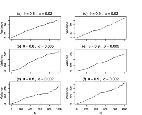
Figure 1: Monte Carlo variance of the derivative approximation in (30) for varying values of $\theta$ and $\sigma$.

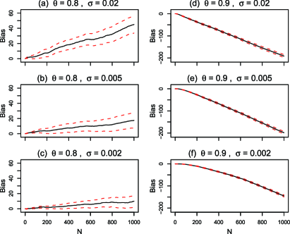
Figure 2: Bias of the derivative approximation in (30) for varying values of $\theta$ and $\sigma$. Dashed lines show pointwise 95% Monte Carlo confidence intervals.

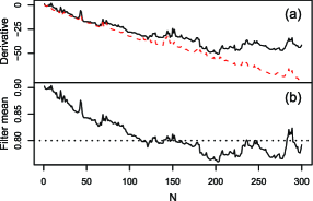
Figure 3: One realization from the simulation study, with $\theta=0.9$ and $\sigma=0.005$. (a) The estimate of $\nabla\ell_{N}(\theta)$ using (30) (solid line) and calculated directly (dashed line). (b) The filter mean $\tilde{\theta}^{F}_{N}$ (solid line) approaching the vicinity of the true parameter value $\theta^{*}=0.8$ (dotted line).

Figures 1 and 2 show how the Monte Carlo variance and the bias vary with $N$ for each value of $\sigma$. These quantities were evaluated from 100 realizations of the model, with 5 replications of the filtering operation per realization, via standard unbiased estimators. We see from Figure 1 that the Monte Carlo variance increases approximately linearly with $N$. This numerical stability is a substantial improvement on the exponential bound guaranteed by Theorem 7. The ordinate values in Figure 1 show that, as anticipated from Theorem 4, the variance increases as $\sigma$ decreases. Figure 2 shows that the bias diminishes as $\sigma$ decreases and is small when $\theta$ is close to $\theta^{*}$. When $\theta$ is distant from $\theta^{*}$, the perturbed parameter values migrate toward $\theta^{*}$ during the course of the filtering operation, as shown in Figure 3(b). Once the perturbed parameters have arrived in the vicinity of $\theta^{*}$, the sum in (30) approximates the derivative of the log likelihood at $\theta^{*}$ rather than at $\theta$. Figure 3(a) demonstrates the resulting bias in the estimate of $\nabla\ell_{N}(\theta)$. However, this bias may be helpful, rather than problematic, for the convergence of the iterated filtering algorithm. The update in (40) is a weighted average of the filtered means of the perturbed parameters. Heuristically, if the perturbed parameters successfully locate a neighborhood of $\theta^{*}$ then this will help to generate a good update for the iterated filtering algorithm. The utility of perturbed parameter values to identify a neighborhood of $\theta^{*}$, in addition to estimating a derivative, does not play a role in our asymptotic justification of iterated filtering. However, it may contribute to the nonasymptotic properties of the method at early iterations.

Appendix: Some standard results on sequential Monte Carlo and stochastic approximation theory

We state some basic theorems that we use to prove Theorems 2, 4 and 5, both for completeness and because we require minor modifications of the standard results. Our goal is not to employ the most recent results available in these research areas, but rather to show that some fundamental and well-known results from both areas can be combined with our Theorems 1 and 3 to synthesize a new theoretical understanding of iterated filtering and iterated importance sampling.

.1 A version of a standard stochastic approximation theorem

We present, as Theorem 6, a special case of Theorem 2.3.1 of Kushner and Clark (1978). For variations and developments on this result, we refer the reader to Kushner and Yin (2003), Spall (2003), Andrieu, Moulines and Priouret (2005) and Maryak and Chin (2008). In particular, Theorem 2.3.1 of Kushner and Clark (1978) is similar to Theorem 4.1 of Spall (2003) and to Theorem 2.1 of Kushner and Yin (2003).

Theorem 6

Let $\ell(\theta)$ be a continuously differentiable function $\mathbb{R}^{p}\to\mathbb{R}$ and let $\{D_{m}(\theta),m\geq 1\}$ be a sequence of independent Monte Carlo estimators of the vector of partial derivatives $\nabla\ell(\theta)$. Define a sequence $\{\hat{\theta}_{m}\}$ recursively by $\hat{\theta}_{m+1}=\hat{\theta}_{m}+a_{m}D_{m}(\hat{\theta}_{m})$. Assume (B1) and (B2) of Section 2 together with the following conditions: [(B5)]

am>0, $a_{m}\to 0$, $\sum_{m}a_{m}=\infty$.

∑mam2sup|θ|<rVarMC(Dm(θ))<∞ for every $r>0$.

limm→∞sup|θ|<r|EMC[Dm(θ)]-∇ℓ(θ)|=0 for every $r>0$. Then $\hat{\theta}_{m}$ converges to $\hat{\theta}=\arg\max\ell(\theta)$ with probability one.

The most laborious step in deducing Theorem 6 from Kushner and Clark (1978) is to check that (B1)–(B5) imply that, for all $\varepsilon>0$,

$$\lim_{n\to\infty}{\mathbb{P}}\Biggl{[}\sup_{j\geq 1}\Biggl{|}\sum_{m=n}^{n+j}a_{m}\{D_{m}(\hat{\theta}_{m})-E_{\mathit{MC}}[D_{m}(\hat{\theta}_{m})\mid\hat{\theta}_{m}]\}\Biggr{|}\geq\varepsilon\Biggr{]}=0,$$ (41)

which in turn implies condition A2.2.4^′′ and hence A2.2.4 of Kushner and Clark (1978). To show (41), we define $\xi_{m}=D_{m}(\hat{\theta}_{m})-E_{\mathit{MC}}[D_{m}(\hat{\theta}_{m})\mid\hat{\theta}_{m}]$ and

$$\xi_{m}^{k}=\cases{\displaystyle\xi_{m},&\quad if $|\hat{\theta}_{m}|\leq k$,\vspace*{1pt}\cr\displaystyle 0,&\quad if $|\hat{\theta}_{m}|>k$.}$$ (42)

Define processes $\{M^{n}_{j}{=}\sum_{m=n}^{n+j}a_{m}\xi_{m},j\geq 0\}$ and $\{M^{n,k}_{j}{=}\sum_{m=n}^{n+j}a_{m}\xi_{m}^{k},j\geq 0\}$ for each $k$ and $n$. These processes are martingales with respect to the filtration defined by the Monte Carlo stochasticity. From the Doob–Kolmogorov martingale inequality [e.g., Grimmett and Stirzaker (1992)],

$${\mathbb{P}}\Bigl{[}\sup_{j}|M^{n,k}_{j}|\geq\varepsilon\Bigr{]}\leq\frac{1}{\varepsilon^{2}}\sum_{m=n}^{\infty}a_{m}^{2}\sup_{|\theta|<k}\operatorname{Var}_{\mathit{MC}}(D_{m}(\theta)).$$ (43)

Define events $F_{n}=\{\sup_{j}|M^{n}_{j}|\geq\varepsilon\}$ and $F_{n,k}=\{\sup_{j}|M^{n,k}_{j}|\geq\varepsilon\}$. It follows from (B4) and (43) that $\lim_{n\to\infty}{\mathbb{P}}\{F_{n,k}\}=0$ for each $k$. In light of the nondivergence assumed in (B2), this implies $\lim_{n\to\infty}{\mathbb{P}}\{F_{n}\}=0$ which is exactly (41).

To expand on this final assertion, let $\Omega=\{\sup_{m}|\hat{\theta}_{m}|<\infty\}$ and $\Omega_{k}=\{\sup_{m}|\hat{\theta}_{m}|<k\}$. Assumption (B2) implies that ${\mathbb{P}}(\Omega)=1$. Since the sequence of events $\{\Omega_{k}\}$ is increasing up to $\Omega$, we have $\lim_{k\rightarrow\infty}{\mathbb{P}}(\Omega_{k})={\mathbb{P}}(\Omega)=1$. Now observe that $\Omega_{k}\cap{F_{n,j}}=\Omega_{k}\cap{F_{n}}$ for all $j\geq{k}$, as there is no truncation of the sequence $\{\xi_{m}^{j},m=1,2,\ldots\}$ for outcomes in $\Omega_{k}$ when $j\geq{k}$. Then,

$$\lim_{n\to\infty}{\mathbb{P}}[F_{n}] \leq \lim_{n\to\infty}{\mathbb{P}}[F_{n}\cap\Omega_{k}]+1-{\mathbb{P}}[\Omega_{k}]$$

$$= \lim_{n\to\infty}{\mathbb{P}}[F_{n,k}\cap\Omega_{k}]+1-{\mathbb{P}}[\Omega_{k}]$$

$$\leq \lim_{n\to\infty}{\mathbb{P}}[F_{n,k}]+1-{\mathbb{P}}[\Omega_{k}]$$

$$= 1-{\mathbb{P}}[\Omega_{k}].$$

Since $k$ can be chosen to make $1-{\mathbb{P}}[\Omega_{k}]$ arbitrarily small, it follows that $\lim_{n\to\infty}{\mathbb{P}}[F_{n}]=0$.

.2 Some standard results on sequential Monte Carlo and importance sampling

A general convergence result on sequential Monte Carlo combining results by Crisan and Doucet (2002) and Del Moral and Jacod (2001) is stated in our notation as Theorem 7 below. The theorem is stated for a POMP model with generic density $\tilde{f}$, parameter vector $\tilde{\theta}$, Markov process $\tilde{X}_{0\dvtx N}$ taking values in $\tilde{{\mathfrak{X}}}^{N+1}$, observation process $\tilde{Y}_{1\dvtx N}$ taking values in ${{\mathfrak{Y}}}^{N}$, and data ${y}^{*}_{1\dvtx N}$. For application to the unperturbed model one sets $\tilde{f}=f$, $\tilde{X}_{n}=X_{n}$, $\tilde{{\mathfrak{X}}}={\mathfrak{X}}$, $\tilde{Y}_{n}=Y_{n}$ and $\tilde{\theta}=\theta$. For application to the stochastically perturbed model one sets $\tilde{f}=g$, $\tilde{X}_{n}=(\breve{X}_{n},\breve{\Theta}_{n})$, $\tilde{{\mathfrak{X}}}={\mathfrak{X}}\times\mathbb{R}^{p}$, $\tilde{Y}_{n}=\breve{Y}_{n}$ and $\tilde{\theta}=(\theta^{[N+1]},\sigma,\tau)$. When applying Theorem 7 in the context of Theorem 4, the explicit expressions for the constants ${C_{26}}$ and ${C_{27}}$ are required to show that the bounds in (45) and (46) apply uniformly for a collection of models indexed by the approximation parameters $\{\tau_{m}\}$ and $\{\sigma_{m}\}$.

Theorem 7 ([Crisan and Doucet (2002); Del Moral and Jacod (2001)])

Let $\tilde{f}$ be a generic density for a POMP model having parameter vector $\tilde{\theta}$, unobserved Markov process $\tilde{X}_{0\dvtx N}$, observation process $\tilde{Y}_{1\dvtx N}$ and data ${y}^{*}_{1\dvtx N}$. Define $\tilde{X}^{F}_{n,j}$ via applying Algorithm 2 with $J$ particles. Assume that $\tilde{f}_{\tilde{Y}_{n}|\tilde{X}_{n}}({y}^{*}_{n}\mid\tilde{x}_{n};\tilde{\theta})$ is bounded as a function of $\tilde{x}_{n}$. For any $\phi\dvtx\tilde{{\mathfrak{X}}}\to\mathbb{R}$, denote the filtered mean of $\phi(\tilde{X}_{n})$ and its Monte Carlo estimate by

$$\phi^{F}_{n}=\int\phi(\tilde{x}_{n})\tilde{f}_{\tilde{X}_{n}|\tilde{Y}_{1\dvtx n}}(\tilde{x}_{n}\mid{y}^{*}_{1\dvtx n};\tilde{\theta})\,d\tilde{x}_{n},\qquad\widetilde{\phi}^{F}_{n}=\frac{1}{J}\sum_{j=1}^{J}\phi(\tilde{X}^{F}_{n,j}).$$ (44)

There are constants ${C_{26}}$ and ${C_{27}}$, independent of $J$, such that

$$E_{\mathit{MC}}[(\widetilde{\phi}^{F}_{n}-\phi^{F}_{n})^{2}] \leq \frac{{C_{26}}\sup_{\tilde{x}}|\phi(\tilde{x})|^{2}}{J},$$ (45)

$$|E_{\mathit{MC}}[\widetilde{\phi}^{F}_{n}-\phi^{F}_{n}]| \leq \frac{{C_{27}}\sup_{\tilde{x}}|\phi(\tilde{x})|}{J}.$$ (46)

Specifically, ${C_{26}}$ and ${C_{27}}$ can be written as linear functions of $1$ and $\eta_{n,1},\ldots,\break\eta_{n,n}$ defined as

$$\eta_{n,i}=\prod_{k=n-i+1}^{n}\biggl{(}\frac{\sup_{\tilde{x}_{k}}\tilde{f}_{\tilde{Y}_{k}|\tilde{X}_{k}}({y}^{*}_{k}\mid\tilde{x}_{k};\tilde{\theta})}{\tilde{f}_{\tilde{Y}_{k}|\tilde{Y}_{1\dvtx k-1}}({y}^{*}_{k}\mid{y}^{*}_{1\dvtx k-1};\tilde{\theta})}\biggr{)}^{2}.$$ (47)

Theorem 2 of Crisan and Doucet (2002) derived (45), and here we start by focusing on the assertion that the constant ${C_{26}}$ in equation (45) can be written as a linear function of $1$ and the quantities $\eta_{n,1},\ldots,\eta_{n,n}$ defined in (47). This was not explicitly mentioned by Crisan and Doucet (2002) but is a direct consequence of their argument. Crisan and Doucet [(2002), Section V] constructed the following recursion, for which $c_{n|n}$ is the constant ${C_{26}}$ in equation (45). For $n=1,\ldots,N$ and $c_{0|0}=0$, define

$$c_{n|n} = \bigl{(}\sqrt{C}+\sqrt{{{\overline{c}}_{n|n}}}\bigr{)}^{2},$$ (48)

$${{\overline{c}}_{n|n}} = 4c_{n|n-1}\biggl{(}\frac{\|\tilde{f}_{\tilde{Y}_{n}|\tilde{X}_{n}}\|}{\tilde{f}_{\tilde{Y}_{n}|\tilde{Y}_{1\dvtx n-1}}({y}^{*}_{n}\mid{y}^{*}_{1\dvtx n-1};\tilde{\theta})}\biggr{)}^{2},$$ (49)

$$c_{n|n-1} = \bigl{(}1+\sqrt{c_{n-1|n-1}}\bigr{)}^{2},$$ (50)

where $\|\tilde{f}_{\tilde{Y}_{n}|\tilde{X}_{n}}\|=\sup_{\tilde{x}_{n}}\tilde{f}_{\tilde{Y}_{n}|\tilde{X}_{n}}({y}^{*}_{n}\mid\tilde{x}_{n};\tilde{\theta})$. Here, $C$ is a constant that depends on the resampling procedure but not on the number of particles $J$. Now, (48)–(50) can be reformulated by routine algebra as

$$c_{n|n} \leq K_{1}+K_{2}{{\overline{c}}_{n|n}},$$ (51)

$${{\overline{c}}_{n|n}} \leq K_{3}q_{n}c_{n|n-1},$$ (52)

$$c_{n|n-1} \leq K_{4}+K_{5}c_{n-1|n-1},$$ (53)

where $q_{n}=\|\tilde{f}_{\tilde{Y}_{n}|\tilde{X}_{n}}\|^{2}[\tilde{f}_{\tilde{Y}_{n}|\tilde{Y}_{1\dvtx n-1}}({y}^{*}_{n}\mid{y}^{*}_{1\dvtx n-1};\tilde{\theta})]^{-2}$ and $K_{1},\ldots,K_{5}$ are constants which do not depend on $\tilde{f}$, $\tilde{\theta}$, ${y}^{*}_{1\dvtx N}$ or $J$. Putting (52) and (53) into (51),

$$c_{n|n} \leq K_{1}+K_{2}K_{3}q_{n}c_{n|n-1}$$

$$\leq K_{1}+K_{2}K_{3}K_{4}q_{n}+K_{2}K_{3}K_{5}q_{n}c_{n-1|n-1}.$$

Since $\eta_{n,i}=q_{n}\eta_{n-1,i}$ for $i<n$, and $\eta_{n,n}=q_{n}$, the required assertion follows from (.2).

To show (46), we introduce the unnormalized filtered mean $\phi^{U}_{n}$ and its Monte Carlo estimate $\widetilde{\phi}^{U}_{n}$, defined by

$$\phi^{U}_{n}=\phi^{F}_{n}\prod_{k=1}^{n}\tilde{f}_{Y_{k}|Y_{1\dvtx k-1}}({y}^{*}_{k}\mid{y}^{*}_{1\dvtx k-1};\tilde{\theta}),\widetilde{\phi}^{U}_{n}=\widetilde{\phi}^{F}_{n}\prod_{k=1}^{n}\frac{1}{J}\sum_{j=1}^{J}w(k,j),$$ (55)

where $w(k,j)$ is computed in step 4 of Algorithm 2 when evaluating $\widetilde{\phi}^{F}_{n}$. Then, Del Moral and Jacod (2001) showed that

$$\quad E_{\mathit{MC}}[\widetilde{\phi}^{U}_{n}] = \phi^{U}_{n},$$ (56)

$$\quad E_{\mathit{MC}}[(\widetilde{\phi}^{U}_{n}-\phi^{U}_{n})^{2}] \leq \frac{({n+1})\sup_{\tilde{x}}|\phi(\tilde{x})|^{2}}{J}\prod_{k=1}^{n}\Bigl{(}\sup_{\tilde{x}_{k}}\tilde{f}_{\tilde{Y}_{k}|\tilde{X}_{k}}({y}^{*}_{k}\mid\tilde{x}_{k};\tilde{\theta})\Bigr{)}^{2}.$$ (57)

We now follow an approach of Del Moral and Jacod [(2001), equation 3.3.14], by defining the unit function $1(\tilde{x})=1$ and observing that $\phi^{F}_{n}=\phi^{U}_{n}/1^{U}_{n}$ and $\widetilde{\phi}^{F}_{n}=\widetilde{\phi}^{U}_{n}/\widetilde{1}^{U}_{n}$. Then (56) implies the identity

$$E_{\mathit{MC}}[\widetilde{\phi}^{F}_{n}-\phi^{F}_{n}]=E_{\mathit{MC}}\biggl{[}(\widetilde{\phi}^{F}_{n}-\phi^{F}_{n})\biggl{(}1-\frac{\widetilde{1}^{U}_{n}}{1^{U}_{n}}\biggr{)}\biggr{]}.$$ (58)

Applying the Cauchy–Schwarz inequality to (58), making use of (45) and (57), gives (46).

We now give a corollary to Theorem 7 for a latent variable model $(\tilde{X},\tilde{Y})$, as defined in Section 2, having generic density $\tilde{f}$, parameter vector $\tilde{\theta}$, unobserved variable $\tilde{X}$ taking values in $\tilde{{\mathfrak{X}}}$, observed variable $\tilde{Y}$ taking values in ${{\mathfrak{Y}}}$, and data ${y}^{*}$. Importance sampling for such a model is a special case of sequential Monte Carlo, with $N=1$ and no resampling step. We present and prove a separate result, which takes advantage of the simplified situation, to make Section 2 and the proof of Theorem 2 self-contained. In the context of Theorem 2, one sets $\tilde{f}=g$, $\tilde{X}=(\breve{X},\breve{\Theta})$, $\tilde{{\mathfrak{X}}}={\mathfrak{X}}\times\mathbb{R}^{p}$, $\tilde{Y}_{n}=\breve{Y}$ and $\tilde{\theta}=(\theta,\tau)$.

Corollary 8

Let $\tilde{f}$ be a generic density for the latent variable model $(\tilde{X},\tilde{Y})$ with parameter vector $\tilde{\theta}$ and data $y^{*}$. Let $\{\tilde{X}_{j},j=1,\ldots,J\}$ be $J$ independent Monte Carlo draws from $\tilde{f}_{\tilde{X}}(\tilde{x};\tilde{\theta})$ and let $w_{j}=\tilde{f}_{\tilde{Y}|\tilde{X}}(y^{*}\mid\tilde{X}_{j};\tilde{\theta})$. Letting $\phi\dvtx\tilde{{\mathfrak{X}}}\to\mathbb{R}$ be a bounded function, write the conditional expectation of $\phi(\tilde{X})$ and its importance sampling estimate as

$$\phi^{C}=\int\phi(\tilde{x}_{n})\tilde{f}_{\tilde{X}|\tilde{Y}}(\tilde{x}\mid{y}^{*};\tilde{\theta})\,d\tilde{x},\widetilde{\phi}^{C}=\frac{\sum_{j=1}^{J}w_{j}\phi(\tilde{X}_{j})}{\sum_{j=1}^{J}w_{j}}.$$ (59)

Assume that $\tilde{f}_{\tilde{Y}|\tilde{X}}({y}^{*}\mid\tilde{x};\tilde{\theta})$ is bounded as a function of $\tilde{x}$. Then,

$$\operatorname{Var}_{\mathit{MC}}(\widetilde{\phi}^{C}) \leq \frac{4\sup_{\tilde{x}}|\phi(\tilde{x})|^{2}\sup_{\tilde{x}}(\tilde{f}_{\tilde{Y}|\tilde{X}}(y^{*}\mid\tilde{x};\tilde{\theta}))^{2}}{J(\tilde{f}_{\tilde{Y}}(y^{*};\tilde{\theta}))^{2}},$$ (60)

$$|E_{\mathit{MC}}[\widetilde{\phi}^{C}]-\phi^{C}| \leq \frac{2\sup_{\tilde{x}}|\phi(\tilde{x})|\sup_{\tilde{x}}(\tilde{f}_{\tilde{Y}|\tilde{X}}(y^{*}\mid\tilde{x};\tilde{\theta}))^{2}}{J(\tilde{f}_{\tilde{Y}}(y^{*};\tilde{\theta}))^{2}}.$$ (61)

We introduce normalized weights $\hat{w}_{j}=w_{j}/\tilde{f}_{\tilde{Y}}(y^{*};\tilde{\theta})$ and a normalized importance sampling estimator $\hat{\phi}^{C}=\frac{1}{J}\sum_{j=1}^{J}\hat{w}_{j}\phi(\tilde{X}_{j})$ to compare to the self-normalized estimator in (59). It is not hard to check that $E_{\mathit{MC}}[\hat{\phi}^{C}]=\phi^{C}$ and $\operatorname{Var}_{\mathit{MC}}(\hat{\phi}^{C})\leq\frac{1}{J}(\sup_{\tilde{x}}|\phi(\tilde{x})|\sup_{\tilde{x}}\tilde{f}_{\tilde{Y}|\tilde{X}}(y^{*}\mid\tilde{x};\tilde{\theta})/\tilde{f}_{\tilde{Y}}(y^{*};\tilde{\theta}))^{2}.$ Now,$\operatorname{Var}_{\mathit{MC}}(\widetilde{\phi}^{C})\leq 2\{\operatorname{Var}_{\mathit{MC}}(\widetilde{\phi}^{C}-\hat{\phi}^{C})+\operatorname{Var}_{\mathit{MC}}(\hat{\phi}^{C})\}$ and

$$\operatorname{Var}_{\mathit{MC}}(\widetilde{\phi}^{C}-\hat{\phi}^{C}) \leq E_{\mathit{MC}}\Biggl{[}\Biggl{(}\frac{({1}/{J})\sum_{j=1}^{J}\hat{w}_{j}\phi(\tilde{X}_{j})}{({1}/{J})\sum_{j=1}^{J}\hat{w}_{j}}-\frac{1}{J}\sum_{j=1}^{J}\hat{w}_{j}\phi(\tilde{X}_{j})\Biggr{)}^{2}\Biggr{]}$$

$$= E_{\mathit{MC}}\Biggl{[}\biggl{(}\frac{({1}/{J})\sum_{j=1}^{J}\hat{w}_{j}\phi(\tilde{X}_{j})}{({1}/{J})\sum_{j=1}^{J}\hat{w}_{j}}\biggr{)}^{2}\Biggl{(}1-\frac{1}{J}\sum_{j=1}^{J}\hat{w}_{j}\Biggr{)}^{2}\Biggr{]}$$

$$\leq \sup_{\tilde{x}}|\phi(\tilde{x})|^{2}E_{\mathit{MC}}\Biggl{[}1-\frac{1}{J}\sum_{j=1}^{J}\hat{w}_{j}\Biggr{]}^{2}$$

$$\leq \frac{\sup_{\tilde{x}}|\phi(\tilde{x})|^{2}\sup_{\tilde{x}}(\tilde{f}_{\tilde{Y}|\tilde{X}}(y^{*}\mid\tilde{x};\tilde{\theta}))^{2}}{J(\tilde{f}_{\tilde{Y}}(y^{*};\tilde{\theta}))^{2}}.$$

This demonstrates (60). To show (61), we write

$$|E_{\mathit{MC}}[\widetilde{\phi}^{C}]-\phi^{C}| = |E_{\mathit{MC}}[\widetilde{\phi}^{C}-\hat{\phi}^{C}]|$$

$$= \Biggl{|}E_{\mathit{MC}}\Biggl{[}(\widetilde{\phi}^{C}-E_{\mathit{MC}}[\widetilde{\phi}^{C}])\Biggl{(}1-\frac{1}{J}\sum_{j=1}^{J}\hat{w}_{j}\Biggr{)}\Biggr{]}\Biggr{|}$$

$$\leq \sqrt{\operatorname{Var}_{\mathit{MC}}(\widetilde{\phi}^{C})\operatorname{Var}_{\mathit{MC}}\Biggl{(}1-\frac{1}{J}\sum_{j=1}^{J}\hat{w}_{j}\Biggr{)}}$$

$$\leq \frac{{2}\sup_{\tilde{x}}|\phi(\tilde{x})|\sup_{\tilde{x}}(\tilde{f}_{\tilde{Y}|\tilde{X}}(y^{*}\mid\tilde{x};\tilde{\theta}))^{2}}{J(\tilde{f}_{\tilde{Y}}(y^{*};\tilde{\theta}))^{2}}.$$

References

- Anderson and Collins (2007) {barticle}[auto:STB—2011-03-03—12:04:44] \bauthor\bsnmAnderson, \bfnmJ. L.\binitsJ. L. and \bauthor\bsnmCollins, \bfnmN.\binitsN. (\byear2007). \btitleScalable implementations of ensemble filter algorithms for data assimilation. \bjournalJournal of Atmospheric and Oceanic Technology \bvolume24 \bpages1452–1463. \endbibitem
- Andrieu, Doucet and Holenstein (2010) {barticle}[auto:STB—2011-03-03—12:04:44] \bauthor\bsnmAndrieu, \bfnmC.\binitsC., \bauthor\bsnmDoucet, \bfnmA.\binitsA. and \bauthor\bsnmHolenstein, \bfnmR.\binitsR. (\byear2010). \btitleParticle Markov chain Monte Carlo methods. \bjournalJ. R. Stat. Soc. Ser. B Stat. Methodol. \bvolume72 \bpages269–342. \endbibitem
- Andrieu, Moulines and Priouret (2005) {barticle}[mr] \bauthor\bsnmAndrieu, \bfnmChristophe\binitsC., \bauthor\bsnmMoulines, \bfnmÉric\binitsÉ. and \bauthor\bsnmPriouret, \bfnmPierre\binitsP. (\byear2005). \btitleStability of stochastic approximation under verifiable conditions. \bjournalSIAM J. Control Optim. \bvolume44 \bpages283–312. \biddoi=10.1137/S0363012902417267, issn=0363-0129, mr=2177157 \endbibitem
- Arulampalam et al. (2002) {barticle}[auto:STB—2011-03-03—12:04:44] \bauthor\bsnmArulampalam, \bfnmM. S.\binitsM. S., \bauthor\bsnmMaskell, \bfnmS.\binitsS., \bauthor\bsnmGordon, \bfnmN.\binitsN. and \bauthor\bsnmClapp, \bfnmT.\binitsT. (\byear2002). \btitleA tutorial on particle filters for online nonlinear, non-Gaussian Bayesian tracking. \bjournalIEEE Trans. Signal Process. \bvolume50 \bpages174–188. \endbibitem
- Bailey (1955) {barticle}[mr] \bauthor\bsnmBailey, \bfnmNorman T. J.\binitsN. T. J. (\byear1955). \btitleSome problems in the statistical analysis of epidemic data. \bjournalJ. Roy. Statist. Soc. Ser. B \bvolume17 \bpages35–58; Discussion 58–68. \bidissn=0035-9246, mr=0073090 \bptnotecheck related \endbibitem
- Bartlett (1960) {bbook}[mr] \bauthor\bsnmBartlett, \bfnmM. S.\binitsM. S. (\byear1960). \btitleStochastic Population Models in Ecology and Epidemiology. \bpublisherMethuen, \baddressLondon. \bidmr=0118550 \endbibitem
- Beyer (2001) {bbook}[mr] \bauthor\bsnmBeyer, \bfnmHans-Georg\binitsH.-G. (\byear2001). \btitleThe Theory of Evolution Strategies. \bpublisherSpringer, \baddressBerlin. \bidmr=1930756 \endbibitem
- Bjørnstad and Grenfell (2001) {barticle}[auto:STB—2011-03-03—12:04:44] \bauthor\bsnmBjørnstad, \bfnmO. N.\binitsO. N. and \bauthor\bsnmGrenfell, \bfnmB. T.\binitsB. T. (\byear2001). \btitleNoisy clockwork: Time series analysis of population fluctuations in animals. \bjournalScience \bvolume293 \bpages638–643. \endbibitem
- Bretó et al. (2009) {barticle}[mr] \bauthor\bsnmBretó, \bfnmCarles\binitsC., \bauthor\bsnmHe, \bfnmDaihai\binitsD., \bauthor\bsnmIonides, \bfnmEdward L.\binitsE. L. and \bauthor\bsnmKing, \bfnmAaron A.\binitsA. A. (\byear2009). \btitleTime series analysis via mechanistic models. \bjournalAnn. Appl. Stat. \bvolume3 \bpages319–348. \biddoi=10.1214/08-AOAS201, issn=1932-6157, mr=2668710 \endbibitem
- Cappé, Godsill and Moulines (2007) {barticle}[auto:STB—2011-03-03—12:04:44] \bauthor\bsnmCappé, \bfnmO.\binitsO., \bauthor\bsnmGodsill, \bfnmS.\binitsS. and \bauthor\bsnmMoulines, \bfnmE.\binitsE. (\byear2007). \btitleAn overview of existing methods and recent advances in sequential Monte Carlo. \bjournalProceedings of the IEEE \bvolume95 \bpages899–924. \endbibitem
- Cappé, Moulines and Rydén (2005) {bbook}[mr] \bauthor\bsnmCappé, \bfnmOlivier\binitsO., \bauthor\bsnmMoulines, \bfnmEric\binitsE. and \bauthor\bsnmRydén, \bfnmTobias\binitsT. (\byear2005). \btitleInference in Hidden Markov Models. \bpublisherSpringer, \baddressNew York. \bidmr=2159833 \endbibitem
- Cauchemez and Ferguson (2008) {barticle}[auto:STB—2011-03-03—12:04:44] \bauthor\bsnmCauchemez, \bfnmS.\binitsS. and \bauthor\bsnmFerguson, \bfnmN. M.\binitsN. M. (\byear2008). \btitleLikelihood-based estimation of continuous-time epidemic models from time-series data: Application to measles transmission in London. \bjournalJournal of the Royal Society Interface \bvolume5 \bpages885–897. \endbibitem
- Celeux, Marin and Robert (2006) {barticle}[mr] \bauthor\bsnmCeleux, \bfnmGilles\binitsG., \bauthor\bsnmMarin, \bfnmJean-Michel\binitsJ.-M. and \bauthor\bsnmRobert, \bfnmChristian P.\binitsC. P. (\byear2006). \btitleIterated importance sampling in missing data problems. \bjournalComput. Statist. Data Anal. \bvolume50 \bpages3386–3404. \biddoi=10.1016/j.csda.2005.07.018, issn=0167-9473, mr=2236856 \endbibitem
- Chopin (2004) {barticle}[mr] \bauthor\bsnmChopin, \bfnmNicolas\binitsN. (\byear2004). \btitleCentral limit theorem for sequential Monte Carlo methods and its application to Bayesian inference. \bjournalAnn. Statist. \bvolume32 \bpages2385–2411. \biddoi=10.1214/009053604000000698, issn=0090-5364, mr=2153989 \endbibitem
- Crisan and Doucet (2002) {barticle}[mr] \bauthor\bsnmCrisan, \bfnmDan\binitsD. and \bauthor\bsnmDoucet, \bfnmArnaud\binitsA. (\byear2002). \btitleA survey of convergence results on particle filtering methods for practitioners. \bjournalIEEE Trans. Signal Process. \bvolume50 \bpages736–746. \biddoi=10.1109/78.984773, issn=1053-587X, mr=1895071 \endbibitem
- Del Moral and Jacod (2001) {bincollection}[mr] \bauthor\bsnmDel Moral, \bfnmPierre\binitsP. and \bauthor\bsnmJacod, \bfnmJean\binitsJ. (\byear2001). \btitleInteracting particle filtering with discrete observations. In \bbooktitleSequential Monte Carlo Methods in Practice (\beditorA. Doucet, \beditorN. de Freitas and \beditorN. J. Gordon, eds.) \bpages43–75. \bpublisherSpringer, \baddressNew York. \bidmr=1847786 \endbibitem
- Diggle and Gratton (1984) {barticle}[mr] \bauthor\bsnmDiggle, \bfnmPeter J.\binitsP. J. and \bauthor\bsnmGratton, \bfnmRichard J.\binitsR. J. (\byear1984). \btitleMonte Carlo methods of inference for implicit statistical models. \bjournalJ. Roy. Statist. Soc. Ser. B \bvolume46 \bpages193–227. \bidissn=0035-9246, mr=0781880 \bptnotecheck related \endbibitem
- Durbin and Koopman (2001) {bbook}[mr] \bauthor\bsnmDurbin, \bfnmJ.\binitsJ. and \bauthor\bsnmKoopman, \bfnmS. J.\binitsS. J. (\byear2001). \btitleTime Series Analysis by State Space Methods. \bseriesOxford Statist. Sci. Ser. \bvolume24. \bpublisherOxford Univ. Press, \baddressOxford. \bidmr=1856951 \endbibitem
- Ergün et al. (2007) {barticle}[pbm] \bauthor\bsnmErgün, \bfnmAyla\binitsA., \bauthor\bsnmBarbieri, \bfnmRiccardo\binitsR., \bauthor\bsnmEden, \bfnmUri T.\binitsU. T., \bauthor\bsnmWilson, \bfnmMatthew A.\binitsM. A. and \bauthor\bsnmBrown, \bfnmEmery N.\binitsE. N. (\byear2007). \btitleConstruction of point process adaptive filter algorithms for neural systems using sequential Monte Carlo methods. \bjournalIEEE Trans. Biomed. Eng. \bvolume54 \bpages419–428. \biddoi=10.1109/TBME.2006.888821, issn=0018-9294, pmid=17355053 \endbibitem
- Fernández-Villaverde and Rubio-Ramírez (2007) {barticle}[mr] \bauthor\bsnmFernández-Villaverde, \bfnmJesús\binitsJ. and \bauthor\bsnmRubio-Ramírez, \bfnmJuan F.\binitsJ. F. (\byear2007). \btitleEstimating macroeconomic models: A likelihood approach. \bjournalRev. Econom. Stud. \bvolume74 \bpages1059–1087. \biddoi=10.1111/j.1467-937X.2007.00437.x, issn=0034-6527, mr=2353620 \endbibitem
- Ferrari et al. (2008) {barticle}[auto:STB—2011-03-03—12:04:44] \bauthor\bsnmFerrari, \bfnmM. J.\binitsM. J., \bauthor\bsnmGrais, \bfnmR. F.\binitsR. F., \bauthor\bsnmBharti, \bfnmN.\binitsN., \bauthor\bsnmConlan, \bfnmA. J. K.\binitsA. J. K., \bauthor\bsnmBjornstad, \bfnmO. N.\binitsO. N., \bauthor\bsnmWolfson, \bfnmL. J.\binitsL. J., \bauthor\bsnmGuerin, \bfnmP. J.\binitsP. J., \bauthor\bsnmDjibo, \bfnmA.\binitsA. and \bauthor\bsnmGrenfell, \bfnmB. T.\binitsB. T. (\byear2008). \btitleThe dynamics of measles in sub-Saharan Africa. \bjournalNature \bvolume451 \bpages679–684. \endbibitem
- Godsill et al. (2007) {barticle}[auto:STB—2011-03-03—12:04:44] \bauthor\bsnmGodsill, \bfnmS.\binitsS., \bauthor\bsnmVermaak, \bfnmJ.\binitsJ., \bauthor\bsnmNg, \bfnmW.\binitsW. and \bauthor\bsnmLi, \bfnmJ.\binitsJ. (\byear2007). \btitleModels and algorithms for tracking of maneuvering objects using variable rate particle filters. \bjournalProceedings of the IEEE \bvolume95 \bpages925–952. \endbibitem
- Grenfell, Bjornstad and Finkenstädt (2002) {barticle}[auto:STB—2011-03-03—12:04:44] \bauthor\bsnmGrenfell, \bfnmB. T.\binitsB. T., \bauthor\bsnmBjornstad, \bfnmO. N.\binitsO. N. and \bauthor\bsnmFinkenstädt, \bfnmB. F.\binitsB. F. (\byear2002). \btitleDynamics of measles epidemics: Scaling noise, determinism, and predictability with the TSIR model. \bjournalEcological Monographs \bvolume72 \bpages185–202. \endbibitem
- Grimmett and Stirzaker (1992) {bbook}[mr] \bauthor\bsnmGrimmett, \bfnmG. R.\binitsG. R. and \bauthor\bsnmStirzaker, \bfnmD. R.\binitsD. R. (\byear1992). \btitleProbability and Random Processes, \bedition2nd ed. \bpublisherThe Clarendon Press/Oxford Univ. Press, \baddressNew York. \bidmr=1199812 \endbibitem
- He, Ionides and King (2010) {barticle}[auto:STB—2011-03-03—12:04:44] \bauthor\bsnmHe, \bfnmD.\binitsD., \bauthor\bsnmIonides, \bfnmE. L.\binitsE. L. and \bauthor\bsnmKing, \bfnmA. A.\binitsA. A. (\byear2010). \btitlePlug-and-play inference for disease dynamics: Measles in large and small towns as a case study. \bjournalJournal of the Royal Society Interface \bvolume7 \bpages271–283. \endbibitem
- Ionides, Bretó and King (2006) {barticle}[pbm] \bauthor\bsnmIonides, \bfnmE. L.\binitsE. L., \bauthor\bsnmBretó, \bfnmC.\binitsC. and \bauthor\bsnmKing, \bfnmA. A.\binitsA. A. (\byear2006). \btitleInference for nonlinear dynamical systems. \bjournalProc. Natl. Acad. Sci. USA \bvolume103 \bpages18438–18443. \biddoi=10.1073/pnas.0603181103, issn=0027-8424, pii=0603181103, pmcid=3020138, pmid=17121996 \endbibitem
- Jensen and Petersen (1999) {barticle}[mr] \bauthor\bsnmJensen, \bfnmJens Ledet\binitsJ. L. and \bauthor\bsnmPetersen, \bfnmNiels Væver\binitsN. V. (\byear1999). \btitleAsymptotic normality of the maximum likelihood estimator in state space models. \bjournalAnn. Statist. \bvolume27 \bpages514–535. \biddoi=10.1214/aos/1018031205, issn=0090-5364, mr=1714719 \endbibitem
- Johannes, Polson and Stroud (2009) {barticle}[auto:STB—2011-03-03—12:04:44] \bauthor\bsnmJohannes, \bfnmM.\binitsM., \bauthor\bsnmPolson, \bfnmN.\binitsN. and \bauthor\bsnmStroud, \bfnmJ.\binitsJ. (\byear2009). \btitleOptimal filtering of jump diffusions: Extracting latent states from asset prices. \bjournalReview of Financial Studies \bvolume22 \bpages2759–2799. \endbibitem
- Johansen, Doucet and Davy (2008) {barticle}[mr] \bauthor\bsnmJohansen, \bfnmAdam M.\binitsA. M., \bauthor\bsnmDoucet, \bfnmArnaud\binitsA. and \bauthor\bsnmDavy, \bfnmManuel\binitsM. (\byear2008). \btitleParticle methods for maximum likelihood estimation in latent variable models. \bjournalStat. Comput. \bvolume18 \bpages47–57. \biddoi=10.1007/s11222-007-9037-8, issn=0960-3174, mr=2416438 \endbibitem
- Keeling and Ross (2008) {barticle}[auto:STB—2011-03-03—12:04:44] \bauthor\bsnmKeeling, \bfnmM.\binitsM. and \bauthor\bsnmRoss, \bfnmJ.\binitsJ. (\byear2008). \btitleOn methods for studying stochastic disease dynamics. \bjournalJournal of the Royal Society Interface \bvolume5 \bpages171–181. \endbibitem
- Kendall et al. (1999) {barticle}[auto:STB—2011-03-03—12:04:44] \bauthor\bsnmKendall, \bfnmB. E.\binitsB. E., \bauthor\bsnmBriggs, \bfnmC. J.\binitsC. J., \bauthor\bsnmMurdoch, \bfnmW. W.\binitsW. W., \bauthor\bsnmTurchin, \bfnmP.\binitsP., \bauthor\bsnmEllner, \bfnmS. P.\binitsS. P., \bauthor\bsnmMcCauley, \bfnmE.\binitsE., \bauthor\bsnmNisbet, \bfnmR. M.\binitsR. M. and \bauthor\bsnmWood, \bfnmS. N.\binitsS. N. (\byear1999). \btitleWhy do populations cycle? A synthesis of statistical and mechanistic modeling approaches. \bjournalEcology \bvolume80 \bpages1789–1805. \endbibitem
- Kiefer and Wolfowitz (1952) {barticle}[mr] \bauthor\bsnmKiefer, \bfnmJ.\binitsJ. and \bauthor\bsnmWolfowitz, \bfnmJ.\binitsJ. (\byear1952). \btitleStochastic estimation of the maximum of a regression function. \bjournalAnn. Math. Statist. \bvolume23 \bpages462–466. \bidissn=0003-4851, mr=0050243 \endbibitem
- King et al. (2008) {barticle}[pbm] \bauthor\bsnmKing, \bfnmAaron A.\binitsA. A., \bauthor\bsnmIonides, \bfnmEdward L.\binitsE. L., \bauthor\bsnmPascual, \bfnmMercedes\binitsM. and \bauthor\bsnmBouma, \bfnmMenno J.\binitsM. J. (\byear2008). \btitleInapparent infections and cholera dynamics. \bjournalNature \bvolume454 \bpages877–880. \biddoi=10.1038/nature07084, issn=1476-4687, pii=nature07084, pmid=18704085 \endbibitem
- Kitagawa (1998) {barticle}[auto:STB—2011-03-03—12:04:44] \bauthor\bsnmKitagawa, \bfnmG.\binitsG. (\byear1998). \btitleA self-organising state-space model. \bjournalJ. Amer. Statist. Assoc. \bvolume93 \bpages1203–1215. \endbibitem
- Kushner and Clark (1978) {bbook}[mr] \bauthor\bsnmKushner, \bfnmHarold J.\binitsH. J. and \bauthor\bsnmClark, \bfnmDean S.\binitsD. S. (\byear1978). \btitleStochastic Approximation Methods for Constrained and Unconstrained Systems. \bseriesAppl. Math. Sci. \bvolume26. \bpublisherSpringer, \baddressNew York. \bidmr=0499560 \endbibitem
- Kushner and Yin (2003) {bbook}[mr] \bauthor\bsnmKushner, \bfnmHarold J.\binitsH. J. and \bauthor\bsnmYin, \bfnmG. George\binitsG. G. (\byear2003). \btitleStochastic Approximation and Recursive Algorithms and Applications, \bedition2nd ed. \bseriesApplications of Mathematics: Stochastic Modelling and Applied Probability \bvolume35. \bpublisherSpringer, \baddressNew York. \bidmr=1993642 \endbibitem
- Laneri et al. (2010) {barticle}[auto:STB—2011-03-03—12:04:44] \bauthor\bsnmLaneri, \bfnmK.\binitsK., \bauthor\bsnmBhadra, \bfnmA.\binitsA., \bauthor\bsnmIonides, \bfnmE. L.\binitsE. L., \bauthor\bsnmBouma, \bfnmM.\binitsM., \bauthor\bsnmYadav, \bfnmR.\binitsR., \bauthor\bsnmDhiman, \bfnmR.\binitsR. and \bauthor\bsnmPascual, \bfnmM.\binitsM. (\byear2010). \btitleForcing versus feedback: Epidemic malaria and monsoon rains in NW India. \bjournalPLoS Comput. Biol. \bvolume6 \bpagese1000898. \endbibitem
- Liu and West (2001) {bincollection}[mr] \bauthor\bsnmLiu, \bfnmJane\binitsJ. and \bauthor\bsnmWest, \bfnmMike\binitsM. (\byear2001). \btitleCombined parameter and state estimation in simulation-based filtering. In \bbooktitleSequential Monte Carlo Methods in Practice (\beditorA. Doucet, \beditorN. de Freitas and \beditorN. J. Gordon, eds.) \bpages197–223. \bpublisherSpringer, \baddressNew York. \bidmr=1847793 \endbibitem
- Maryak and Chin (2008) {barticle}[mr] \bauthor\bsnmMaryak, \bfnmJohn L.\binitsJ. L. and \bauthor\bsnmChin, \bfnmDaniel C.\binitsD. C. (\byear2008). \btitleGlobal random optimization by simultaneous perturbation stochastic approximation. \bjournalIEEE Trans. Automat. Control \bvolume53 \bpages780–783. \biddoi=10.1109/TAC.2008.917738, issn=0018-9286, mr=2401029 \endbibitem
- Morton and Finkenstädt (2005) {barticle}[mr] \bauthor\bsnmMorton, \bfnmAlexander\binitsA. and \bauthor\bsnmFinkenstädt, \bfnmBärbel F.\binitsB. F. (\byear2005). \btitleDiscrete time modelling of disease incidence time series by using Markov chain Monte Carlo methods. \bjournalJ. Roy. Statist. Soc. Ser. C \bvolume54 \bpages575–594. \biddoi=10.1111/j.1467-9876.2005.05366.x, issn=0035-9254, mr=2137255 \endbibitem
- Newman et al. (2009) {barticle}[mr] \bauthor\bsnmNewman, \bfnmKen B.\binitsK. B., \bauthor\bsnmFernández, \bfnmCarmen\binitsC., \bauthor\bsnmThomas, \bfnmLen\binitsL. and \bauthor\bsnmBuckland, \bfnmStephen T.\binitsS. T. (\byear2009). \btitleMonte Carlo inference for state-space models of wild animal populations. \bjournalBiometrics \bvolume65 \bpages572–583. \biddoi=10.1111/j.1541-0420.2008.01073.x, issn=0006-341X, mr=2751482 \bptnotecheck year \endbibitem
- Qian and Shapiro (2006) {barticle}[mr] \bauthor\bsnmQian, \bfnmZhiguang\binitsZ. and \bauthor\bsnmShapiro, \bfnmAlexander\binitsA. (\byear2006). \btitleSimulation-based approach to estimation of latent variable models. \bjournalComput. Statist. Data Anal. \bvolume51 \bpages1243–1259. \biddoi=10.1016/j.csda.2006.02.016, issn=0167-9473, mr=2297520 \endbibitem
- Reuman et al. (2006) {barticle}[pbm] \bauthor\bsnmReuman, \bfnmDaniel C.\binitsD. C., \bauthor\bsnmDesharnais, \bfnmRobert A.\binitsR. A., \bauthor\bsnmCostantino, \bfnmRobert F.\binitsR. F., \bauthor\bsnmAhmad, \bfnmOmar S.\binitsO. S. and \bauthor\bsnmCohen, \bfnmJoel E.\binitsJ. E. (\byear2006). \btitlePower spectra reveal the influence of stochasticity on nonlinear population dynamics. \bjournalProc. Natl. Acad. Sci. USA \bvolume103 \bpages18860–18865. \biddoi=10.1073/pnas.0608571103, issn=0027-8424, pii=0608571103, pmcid=1693752, pmid=17116860 \endbibitem
- Rogers and Williams (1994) {bbook}[mr] \bauthor\bsnmRogers, \bfnmL. C. G.\binitsL. C. G. and \bauthor\bsnmWilliams, \bfnmDavid\binitsD. (\byear1994). \btitleDiffusions, Markov Processes, and Martingales. Vol. 1: Foundations, \bedition2nd ed. \bpublisherWiley, \baddressChichester. \bidmr=1331599 \endbibitem
- Spall (2003) {bbook}[mr] \bauthor\bsnmSpall, \bfnmJames C.\binitsJ. C. (\byear2003). \btitleIntroduction to Stochastic Search and Optimization: Estimation, Simulation, and Control. \bpublisherWiley-Interscience, \baddressHoboken, NJ. \biddoi=10.1002/0471722138, mr=1968388 \endbibitem
- Toni et al. (2008) {barticle}[auto:STB—2011-03-03—12:04:44] \bauthor\bsnmToni, \bfnmT.\binitsT., \bauthor\bsnmWelch, \bfnmD.\binitsD., \bauthor\bsnmStrelkowa, \bfnmN.\binitsN., \bauthor\bsnmIpsen, \bfnmA.\binitsA. and \bauthor\bsnmStumpf, \bfnmM. P.\binitsM. P. (\byear2008). \btitleApproximate Bayesian computation scheme for parameter inference and model selection in dynamical systems. \bjournalJournal of the Royal Society Interface \bvolume6 \bpages187–202. \endbibitem
- West and Harrison (1997) {bbook}[mr] \bauthor\bsnmWest, \bfnmMike\binitsM. and \bauthor\bsnmHarrison, \bfnmJeff\binitsJ. (\byear1997). \btitleBayesian Forecasting and Dynamic Models, \bedition2nd ed. \bpublisherSpringer, \baddressNew York. \bidmr=1482232 \endbibitem