Design and performance evaluation of a state-space based AQM

Abstract

Recent research has shown the link between congestion control in communication networks and feedback control system. In this paper, the design of an active queue management (AQM) which can be viewed as a controller, is considered. Based on a state space representation of a linearized fluid flow model of TCP, the AQM design is converted to a state feedback synthesis problem for time delay systems. Finally, an example extracted from the literature and simulations via a network simulator NS (under cross traffic conditions) support our study.

1 Introduction

Congestion control is a very active research area in network community. In order to supply the well known transmission control protocol (TCP), active queue management mechanisms have been developed. AQM regulates the queue length of a router by actively dropping packets. Various mechanisms have been proposed in the literature such as Random Early Detection (RED) [4], Random Early Marking (REM) [1], Adaptive Virtual Queue (AVQ) [10] and many others [19]. Their performances have been evaluated in [19] and empirical studies have shown their effectiveness (see [12]). Recently, significant studies proposed by [7] have redesigned the AQMs using control theory and $P$, $PI$ have been developed in order to cope with the packet dropping problem. Then, using dynamical model developed by [16], many research have been devoted to deal with congestion problem in a control theory framework (for example see [22]). Nevertheless, most of these papers do not take into account the delay and ensure the stability in closed-loop for all possible delays which could be conservative in practice.
Modeling the congestion control using time delay is not new and global stability analysis has been studied by [15] and [17] via Lyapunov-Krasovskii theory. Also, in [9], a delay dependent state feedback controller is provided by compensation of the delay with a memory feedback control. This latter methodology is interesting in theory but hardly suitable in practice.
Based on a recently developed Lyapunov-Krasovskii functional, an AQM stabilizing the TCP model is designed. This synthesis problem is carried out as state feedback synthesis for time delay systems. Then, this method is applied on an augmented system in order to vanish the steady state error in spite of disturbance.
The paper is organized as follows. The second part presents the model of a network supporting TCP and the time delay system representation. Section 3 is dedicated to the design of the AQM ensuring the stabilization of TCP. Section 4 presents application of the exposed theory and simulation results using NS-2 (see [3]) before concluding this work.

2 Problem statement

2.1 The linearized TCP fluid-flow model

In this paper, we consider the network topology consisting of $N$ homogeneous TCP sources (i.e with the same propagation delay) connected to a destination node through a router (see figure 1).

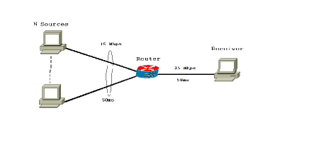
Figure 1: Network configuration

The bottleneck link is shared by $N$ flows and TCP applies the well known congestion avoidance algorithm to cope with the phenomenon of congestion collapse [8]. Many studies have been dedicated to the modeling of TCP and its AIMD (additive-increase multiplicative-deacrease) behavior [13], [21], [22] and references therein. We consider in this note the model (1) developed by [16]. This latter may not capture with high accuracy the dynamic behavior of TCP but its simplicity allows us to apply our methodology. Let consider the following model

$$\left\{\begin{array}[]{rcl}\dot{W}(t)&=&\frac{1}{R(t)}-\frac{W(t)W(t-R(t))}{2R(t-R(t))}p(t-R(t))\\ \dot{q}(t)&=&\frac{W(t)}{R(t)}N-C+d(t)\end{array}\right.$$ (1)

where $W$ is the TCP window size, $q$ is the queue length of the router buffer, $R$ is the round trip time (RTT) and can be expressed as $R=q/C+T_{p}$. $C$, $T_{p}$ and $N$ are parameters related to the network configuration and represent the transmission capacity of the router, the propagation delay and the number of TCP sessions respectively. The variable $p$ is the marking/dropping probability of a packet (that depends whether the ECN option, explicit congestion notification, is enabled, see [18]). In the mathematical model (1), we have introduced an additional signal $d(t)$ which models cross traffics through the router and filling the buffer. These traffics are not TCP based flows (not modeled in TCP dynamic) and can be viewed as perturbations since they are not reactive to packets dropping (for example, UDP based traffic). A linearization and some simplifications of (1) was carried out in [7] to allow the use of traditional control theory approach. The linearized fluid-flow model of TCP is as follow,

$$\left\{\begin{array}[]{ll}\delta\dot{W}(t)=-\frac{N}{R_{0}^{2}C}\Big{(}\delta W(t)+\delta W(t-h(t))\Big{)}\\ \hskip 19.91684pt-\frac{1}{R_{0}^{2}C}\Big{(}\delta q(t)-\delta q(t-h(t))\Big{)}-\frac{R_{0}C^{2}}{2N^{2}}\delta p(t-h(t))\\ \delta\dot{q}(t)=\frac{N}{R_{0}}\delta W(t)-\frac{1}{R_{0}}\delta q(t)+d(t)\end{array}\right.$$ (2)

where $\delta W\doteq W-W_{0}$, $\delta q\doteq q-q_{0}$ and $\delta p\doteq p-p_{0}$ are the perturbated variables about the operating point. The operating point $(W_{0},q_{0},p_{0})$ is defined by

$$\left\{\begin{array}[]{l}\dot{W}=0~{}\Rightarrow~{}W_{0}^{2}p_{0}=2\\ \dot{q}=0~{}\Rightarrow~{}W_{0}=\frac{R_{0}C}{N},~{}R_{0}=\frac{q_{0}}{C}+T_{p}\end{array}\right.$$

The input of the model (2) corresponds to the drop probability of a packet. This probability is fixed by the AQM. This latter has for objective to regulate the queue size of the router buffer. In this paper, this regulation problem is addressed in Section 3 with the design of a stabilizing state feedback for time delay systems. Indeed, an AQM acts as a controller (see figure 2) and in order to design it, we have to solve a synthesis problem. Considering a state feedback, the queue management strategy of the drop probability will be expressed as

$$p(t)=p_{0}+k_{1}\delta W(t)+k_{2}\delta q(t).$$ (3)

where $k_{1}$ and $k_{2}$ are the components of the matrix gain $K$ which we have to design. Note that the input $p(t)=u(t)+p_{0}$ of the system (4) is delayed.

\psfrag{p0}[0.7]{$p_{0}$}\psfrag{W0}[0.7]{$W_{0}$}\psfrag{deltaq}[0.7]{$\delta q(t)$}\includegraphics[height=85.35826pt,width=156.49014pt]{schema_SF}

Figure 2: Design of an AQM as a state feedback

2.2 Time delay system approach

In this paper, we choose to model the dynamics of the queue and the congestion window as a time delay system. Indeed, the delay is an intrinsic phenomenon in networks and taking into account its characteristic should improve the precision of our model with respect to the TCP behavior.
The linearized TCP fluid model (2) can be rewritten as the following time delay system:

$$\left\{\begin{array}[]{l}\dot{x}(t)=Ax(t)+A_{d}x(t-h)+Bu(t-h)+B_{d}d(t)\\ x_{0}(\theta)=\phi(\theta),~{}\mbox{with }\theta\in[-h,0]\end{array}\right.$$ (4)

with

$${\small A\!=\!\left[\begin{array}[]{cc}\!-\frac{N}{R_{0}^{2}C}\!&\!-\frac{1}{CR_{0}^{2}}\!\\ \!\frac{N}{R_{0}}\!&\!-\frac{1}{R_{0}}\!\end{array}\right]\!,\!~{}A_{d}\!=\!\left[\begin{array}[]{cc}\!-\frac{N}{R_{0}^{2}C}\!&\!\frac{1}{R_{0}^{2}C}\!\\ \!0\!&\!0\!\end{array}\right]\!,\!B\!=\!\left[\begin{array}[]{c}\!-\frac{C^{2}R_{0}}{2N^{2}}\!\\ \!0\!\end{array}\right]\!}$$ (5)

$B_{d}=[0~{}~{}1]^{T}$, $x(t)=[\delta W(t)~{}~{}\delta q(t)]^{T}$ is the state vector and $u(t)=\delta p(t)$ the input. $\phi(\theta)$ is the initial condition.
There are mainly three methods to study time delay system stability: analysis of the characteristic roots, robust approach and Lyapunov theory. The latter will be considered because it is an effective and practical method which provides LMI and BMI (Linear/Bilinear Matrix Inequalities, [2]) criteria. To analyze and control the system (4), the Lyapunov-Krasovskii approach (see [6]) is used which is an extension of the traditional Lyapunov theory.

3 Stabilization: design of an AQM

In Section 2, the model of TCP/AQM has been addressed as time delay system. The congestion problem needs the construction of a controller which regulates the buffer queue length. In this section, we are first going to present a delay dependent stability analysis condition for time delay systems. Then, based on this criterion, a synthesis method to derive a stabilizing state feedback is deduced.

3.1 Stability analysis of time delay systems

In this subsection, our goal is to derived a condition which takes into account an upperbound of the delay. The delay dependent case starts from a system stable without delays and looks for the maximal delay that preserves stability.
Usually, all methods involve a Lyapunov functional, and more or less tight techniques to bound some cross terms and to transform system [6]. These choices of specific Lyapunov functionals and overbounding techniques are the origin of conservatism. In the present paper, we choose a recently developed Lyapunov-Krasovskii functional (6) [5]:

$$\begin{array}[]{c}V(x_{t})=x^{T}(t)Px(t)+\int\limits_{t-\frac{h}{r}}^{t}\!\!\int\limits_{\theta}^{t}\dot{x}^{T}(s)R\dot{x}(s)dsd\theta\\[5.0pt] ~{}~{}~{}~{}~{}+\int_{t-\frac{h}{r}}^{t}\left(\begin{array}[]{c}x(s)\\ x(s-\frac{1}{r}h)\\ \vdots\\ x(s-\frac{r-1}{r}h)\end{array}\right)^{T}Q\left(\begin{array}[]{c}x(s)\\ x(s-\frac{1}{r}h)\\ \vdots\\ x(s-\frac{r-1}{r}h)\end{array}\right)ds\end{array}$$ (6)

where $P\in\sf{S}^{n}$ is a positive definite matrix, $Q\in\sf{S}^{rn}$ and $R\in\sf{S}^{n}$ are two positive definite matrices. $r\geq 1$ is an integer corresponding to the discretization step. Using this functional, Let us introduce the following proposition.

Proposition 1

If there exist symmetric positive definite matrices $P$, $R\in\sf{R}^{n\times n}$, $Q\in\sf{R}^{rn\times rn}$, a scalar $h_{m}>0$ and an integer $r\geq 1$ such that

$$S^{\perp^{T}}\Gamma S^{\perp}<\sf{0}$$ (7)

where

$${\tiny\Gamma=\!\left[\begin{array}[]{ccccc}\frac{h_{m}}{r}{\bf R}&{\bf P}&\sf{0}&\ldots&\sf{0}\\ {\bf P}&-\frac{r}{h_{m}}{\bf R}&\frac{r}{h_{m}}{\bf R}&{}\hfil&\vdots\\ \sf{0}&\frac{r}{h_{m}}{\bf R}&-\frac{r}{h_{m}}{\bf R}&{}\hfil&\vdots\\ \vdots&{}\hfil&{}\hfil&\ddots&\vdots\\ \sf{0}&\ldots&\ldots&\ldots&\sf{0}\end{array}\right]+\left[\begin{array}[]{ccc}\sf{0}&\ldots&\sf{0}\\ \vdots&{\bf Q}&\vdots\\ \sf{0}&\ldots&\sf{0}\end{array}\right]+\left[\begin{array}[]{cc}\sf{0}&\ldots\\ \sf{0}&\ldots\\ \vdots&{\bf Q}\end{array}\right]}$$ (8)

and

$$S=\left[\begin{array}[]{cccc}-\sf{1}&A&\sf{0}_{n\times(r-1)n}&A_{d}\end{array}\right]$$ (9)

then, system (4) (with $u(t)=0$ and $d(t)=0$) is stable for all $h\leq h_{m}$.

Proof: It is always possible to rewrite (4) as $S\xi=\sf{0}$ where

$$\begin{array}[]{c}\xi=\left[\begin{array}[]{c}\dot{x}(t)\\ x(t)\\ x(t-\frac{1}{r}h)\\ \vdots\\ x(t-\frac{r-1}{r}h)\\ x(t-h)\end{array}\right]\in\sf{R}^{(r+2)n}\end{array}$$ (10)

and $S$ is defined as (9). Using the extended variable $\xi(t)$ (10), the derivative of $V$ along the trajectories of system (4) leads to:

$$\left\{\begin{array}[]{rcl}\dot{V}(x_{t})&=&\xi^{T}\left[\begin{array}[]{ccccc}\frac{h}{r}{\bf R}&{\bf P}&\sf{0}&\ldots&\sf{0}\\ {\bf P}&-\frac{r}{h}{\bf R}&\frac{r}{h}{\bf R}&{}\hfil&\vdots\\ \sf{0}&\frac{r}{h}{\bf R}&-\frac{r}{h}{\bf R}&{}\hfil&\vdots\\ \vdots&{}\hfil&{}\hfil&\ddots&\vdots\\ \sf{0}&\ldots&\ldots&\ldots&\sf{0}\end{array}\right]\xi\\[5.0pt] &+&\xi^{T}\left[\begin{array}[]{ccc}\sf{0}&\ldots&\sf{0}\\ \vdots&{\bf Q}&\vdots\\ \sf{0}&\ldots&\sf{0}\end{array}\right]\xi-\xi^{T}\left[\begin{array}[]{cc}\sf{0}&\ldots\\ \sf{0}&\ldots\\ \vdots&{\bf Q}\end{array}\right]\xi<\sf{0}\\[5.0pt] \mbox{s.t.}&&\left[\begin{array}[]{cccccc}-\sf{1}&A&\sf{0}&\cdots&\sf{0}&A_{d}\end{array}\right]\xi=0\end{array}\right.$$ (11)

$$\Leftrightarrow\left\{\begin{array}[]{ll}\dot{V}(x_{t})=\xi^{T}\Gamma\xi<\sf{0}\\ \mbox{s.t. }\left[\begin{array}[]{cccccc}-\sf{1}&A&\sf{0}&\cdots&\sf{0}&A_{d}\end{array}\right]\xi=0\end{array}\right.$$ (12)

where $\Gamma\in\sf{S}^{(r+2)n}$ depends on $P$, $R$, $Q$ and the delay $h$.
Using projection lemma [20], expression (12) is equivalent to (7).  
Remark 1:

• There exists another equivalent form of this LMI provided in [5] and based on quadratic separation.

• In the same paper, it is shown that for $r=1$, this proposed function (6) is equivalent to the main classical results of the literature. Moreover, it is also proved that for $r>1$ conservatism is reduced.

3.2 A first result on synthesis

Given the analysis condition (7) and applying the delayed state feedback (3) on system (4) (in this subsection, the disturbance is not taken into account), the following proposition is obtained.

Proposition 2

If there exist symmetric positive definite matrices $P$, $R\in\sf{R}^{n\times n}$, $Q\in\sf{R}^{rn\times rn}$, a matrix $X\in\sf{R}^{(r+2)n\times n}$, a scalar $h_{m}>0$, an integer $r\geq 1$ and a matrix $K\in\sf{R}^{m\times n}$ such that

$$\Gamma+{\bf X}S+S^{T}{\bf X}^{T}<\sf{0}$$ (13)

where $\Gamma$ is defined as (8) and

$$S=\left[\begin{array}[]{cccc}-\sf{1}&A&\sf{0}_{n\times(r-1)n}&A_{d}+B{\bf K}\end{array}\right]$$ (14)

then, system (4) can be stabilized for all $h\leq h_{m}$ for the control law $u(t)=Kx(t)$ (and for $d(t)=0$).

Proof: Considering the system (4) with the state feedback (3), the following interconnected system is deduced

$$\dot{x}(t)=Ax(t)+\bar{A}_{d}x(t-h),$$ (15)

where $\bar{A}_{d}=A_{d}+BK$ and $A$, $A_{d}$ and $B$ are defined as (5). Then, we can apply the analysis condition (7) on (15). Using Finsler lemma [20], there exists a matrix $X\in\sf{R}^{(r+2)n\times n}$ such that if (13) is satisfied then (7) is true. Matrix $X$ is called “slack variables”which can reduced conservatism and may be interesting for synthesis purpose as well as robust control purpose.  
Remark 2:

• To solve the synthesis criterion (13), one has to use a BMI solver.

• In [11], a relaxation algorithm is provided with LMI condition to find a stabilizing state feedback.

3.3 Delay dependent state feedback with an integral action

In the previous section, the design of a state feedback control for time delay systems has been exposed. The use of a such controller has been carried out in [11]. However, it appears that in some cases, the queue size is no longer regulated at the desired level (this phenomenon is only observed on the network simulator NS). It thus appears a slight steady state error which can be explain by an inaccuracy of the model. Futhermore, the introduction of non responsive flows like UDP (user datagram protocol) traffics which appear as a disturbance affects the queue size equilibrium and changes the steady state. In order to overcome these problems, the AQM is supplemented with an integral action. The idea is to apply the previously exposed synthesis method over an augmented time delay system composed of the original system (4) and an integrator (see figure 3). The augmented system has the following form

$$\dot{z}=\left[\begin{array}[h]{cc}A&\begin{array}[h]{c}0\\ 0\end{array}\\ \begin{array}[h]{cc}0&1\end{array}&0\end{array}\right]z(t)+\left[\begin{array}[h]{cc}A_{d}&\begin{array}[h]{c}0\\ 0\end{array}\\ \begin{array}[h]{cc}0&0\end{array}&0\end{array}\right]z(t-h)$$ (16)

$+\left[\begin{array}[h]{c}B\\ 0\end{array}\right]\delta p(t-h)$
with $z^{T}=[\delta W~{}~{}\delta q~{}~{}u]^{T}$ is the extended state variable. Then, the global control which correspond to our AQM, is a dynamic state feedback

$$\delta p(t)=K\left[\begin{array}[]{c}\delta W(t)\\ \delta q(t)\\ u(t)\end{array}\right]=k_{1}\delta W(t)+k_{2}\delta q(t)+k_{3}\int_{0}^{t}\delta q(t)dt.$$ (17)

\psfrag{p0}[0.7]{$p_{0}$}\psfrag{W0}[0.7]{$W_{0}$}\psfrag{deltaq}[0.7]{$\delta q(t)$}\includegraphics[height=85.35826pt,width=156.49014pt]{schema_SFI}

Figure 3: Design of an AQM as a dynamic state feedback

In our problem, non modelled crossing traffics $d(t)$ such as UDP based applications are introduced as exogenous signals (see figures 2 and 3). The queue dynamic is modified as

$$\dot{q}(t)=\frac{W(t)}{R(t)}N-C+d(t)$$ (18)

Considering equations (17), the first equation of (2) and (18), we obtain the transfer function $T(s)$ from the disturbance $D(s)$ to the queue size (about the operating point) $\Delta Q(s)$:

$$T(s)=\frac{b(s)s}{(s+\frac{1}{R_{0}})sb(s)+\frac{N}{R_{0}}\left[\frac{s}{R_{0}^{2}C}(1-e^{-hs})+a(s)sk_{2}+a(s)k_{3}\right]},$$ (19)

with $a(s)=-\frac{R_{0}C^{2}}{2N^{2}}e^{-hs}$ and $b(s)=s+\frac{N}{R_{0}^{2}C}(1+e^{-hs})+a(s)k_{1}$. It can be easily shown that for a step type disturbance, the queue size still converges to its equilibrium.

3.4 Estimation of the congestion window

In these last two parts, a state feedback synthesis has been performed for the congestion control of TCP flows and the management of the router buffer. So far we have considered that the whole state was accessible. However, although the congestion window can be measured in NS (few lines have to be added in the TCP code), it is not the case in reality. That’s why, in this paper it is proposed to estimate this latter variable using the aggregate flow incoming to the router buffer. The sending rate of single TCP source can be approximated by

$$x_{i}(t)=\frac{W(t)}{R(t)}.$$ (20)

The above approximation is valid as long as the model does not describe the communication at a finer time scale than few round trip time (see [13]). Consequently, the whole incoming rate observed by the router is $x(t)=NW(t)/R(t)$. The measure of the aggregate flow has already been proposed and successfully exploited in [10] and [9] for the realization of the AVQ and a PID type AQM respectively. It is worth noting that queue-based AQMs like RED or PI can be assimilated as output feedbacks according to the queue length. Conversely, AVQ can be viewed as an output feedback with respect to the aggregate flow, belonging thus to the rate-based AQM class.

4 NS-2 simulations

As a widely adopted numerical illustration extracted from [7] (see figure 1 for the network topology), consider the case where $q_{0}=175$ packets, $T_{p}=0.2$ second and $C=3750$ packets/s (corresponds to a $15$ Mb/s link with average packet size $500$ bytes). Then, for a load of $N=60$ TCP sessions, we have $W_{0}=15$ packets, $p_{0}=0.008$, $R_{0}=0.246$ seconds. According to the synthesis criteria presented in Section 3, the state feedback matrices

$$K_{SF}=10^{-3}\left[\begin{array}[h]{c}-0.2372\\ 0.0429\end{array}\right]\mbox{ and }K_{SFI}=10^{-4}\left[\begin{array}[h]{c}0.9385\\ 0.5717\\ 0.3559\end{array}\right]$$ (21)

are calculated for the construction of the control laws (3) and (17) respectively.
We aim at proving the effectiveness of our method using NS-2 [3], a network simulator widely used in the communication networks community. Taking values from the previous numerical example, we apply the new AQM based on a state feedback. The target queue length $q_{0}$ is $175$ packets while buffer size is $800$. The average packet length is $500$ bytes. The default transport protocol is TCP-New Reno without ECN marking.
For the convenience of comparison, we adopt the same values and network configuration than [7] who design a PI controller (Proportional-Integral). This PI is configured as follow, the coefficients $a$ and $b$ are fixed at $1.822e-5$ and $1.816e-5$ respectively, the sampling frequency is $160$Hz. The RED has been also tested using the parametric configuration recommended in [7]. In figure 4, simulations are performed under an external perturbation. This latter is composed of 7 additional sources (CBR applications over UDP protocol) sending 1000 bytes packet length with a 1Mbytes/s throughput between $t=40s$ and $t=100s$. The two DSF (see figure 4 for the DSF based on the congestion window and the aggregate flow) regulate faster than others and are able to reject the disturbance swiftly. Conversely, figure 4 shows the time response of the queue length with a simple state feedback $K_{SF}$ (3) as an AQM. One can note that the queue is stabilized slightly above the desired level (around $200$ pkts). Futhermore, the non reponsive cross traffic affects the steady state. The table 1 summarizes the benefits of the two $K_{SFI}$ AQMs (according to simulations with UDP cross traffics). Classical statistical characteristics are calculated during the whole simulation, then only during the UDP cross traffic and finally after the UDP cross traffic (come back to steady state). These characteristics are mean, standard deviation ($Sdt$) and the square of the variation coefficient ($CV2=(Std/mean)^{2}$). This latter calculation assess the relative dispersion of the queue length around its mean. The mean points out the control precision and the standard deviation shows the ability of the AQM to keep the queue size close to its equilibrium. In table 1, we can observe that $K_{SFI}(cwnd)$ maintains a very good control on the buffer queue during the whole simulation. Even though $K_{SFI}(aggfl)$ is slightly slower than the previous one, statistics (Std and CV2) show again a good regulation. Although PI reject the perturbation quite fast, extensive fluctuations appear during the steady state. To conclude, the two DSF are efficient AQMs which provide the best precision and are able to regulate faster and closer to the mean compared to others AQMs.

​AQMs​	RED	PI	$K_{SF}$	​​​​$K_{SFI}$​​​​ ​​​​(cwnd)​​​​	​​​​$K_{SFI}$​​​​ ​​​​(aggfl)​​​​
​Mean​	235.7	176.7	263.9	​​​​ 175.9​​​​	​​​​ 175.5​​​​	B
​Sdt​	112.40	71.19	78.59	​​​​ 54.57​​​​	​​​​ 63.64​​​​	B
​CV2​	0.227	0.162	0.088	​​​​ 0.096​​​​	​​​​ 0.131​​​​	B
​Mean​	270.3	178.3	338.0	​​​​ 173.4​​​​	​​​​ 175.6​​​​	D
​Sdt​	57.39	40.42	41.21	​​​​ 35.08​​​​	​​​​ 28.32​​​​	D
​CV2​	0.045	0.051	0.014	​​​​ 0.040​​​​	​​​​ 0.026​​​​	D
​Mean​	201.4	177.8	236.0	​​​​ 176.2​​​​	​​​​174.8​​​	A
​Sdt​	22.24	36.64	30.48	​​​​ 30.22​​​​	​​​​ 32.64​​​​	A
​CV2​	0.012	0.042	0.016	​​​​ 0.029​​​​	​​​​ 0.034​​​​	A

Table 1: Statistical characteristics for different AQMs (units are pkts) at different periods (B, D and A: before, during and after CBR applications)

To complete our simulation, we propose another NS-2 simulation between different AQMs: REM, AVQ, RED, PI, KSFI(cwnd) and KSFI(aggfl). We consider different levels of CBR cross traffics (13 sources, 1Mb). RED, REM, PI and AVQ are fixed to same values as in [14], which is a performance analysis of AQM under DoS attacks. The additional sources are sending 1000 bytes packet length with a 1Mbytes/s throughput between $t=60s$ and $t=180s$. The simulation is illustrated in the figure 5. In these last two cases, one can imagine that AQMs could detect cross traffics or traffic anomalies. Moreover, $AQM=\{K_{SFI(cwnd)},K_{SFI(Aggfl)}\}$ still have well behaviours under cross traffic conditions.

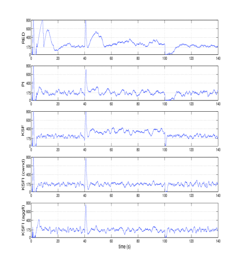
Figure 4: Time evolution of the queue length, $AQM=\{RED,PI,K_{SF},K_{SFI(cwnd)},K_{SFI(Aggfl)}\}$ under UDP crossing traffic

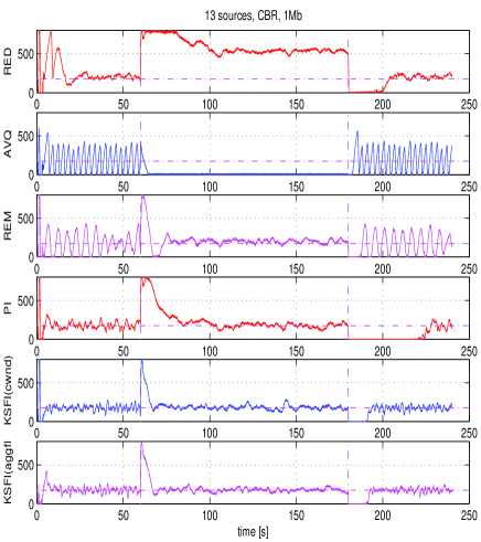
Figure 5: Time evolution of the queue length, $AQM=\{RED,AVQ,REM,PI,K_{SFI(cwnd)},K_{SFI(Aggfl)}\}$ under cross traffic

5 Conclusion

In this preliminary work, we have proposed the design of an AQM for the congestion control in communications networks. The developed AQM has been constructed using a dynamic state feedback control law. An integral action has been added to reject the steady state error in spite of disturbance, $d(t)$ (cross traffic). Finally, the AQM has been validated using NS simulator. Future work consist in the improvement about control laws (theoritical part) extended to a greater network using a decentralized approach to reduce the weakness of this method on one side and validation on emulation platform (experimental part) on the other side.

References

- [1] S. Athuraliya, D. Lapsley, and S. Low. An enhanced random early marking algorithm for internet flow control. In IEEE INFOCOM, pages 1425–1434, December 2000.
- [2] S. Boyd, L. El Ghaoui, E. Feron, and V. Balakrishnan. Linear Matrix Inequalities in System and Control Theory. SIAM, Philadelphia, USA, 1994. in Studies in Applied Mathematics, vol.15.
- [3] K. Fall and K. Varadhan. The ns manual. notes and documentation on the software ns2-simulator, 2002. URL: www.isi.edu/nsnam/ns/.
- [4] S. Floyd and V. Jacobson. Random early detection gateways for congestion avoidance. IEEE/ACM Transactions on Networking, 1:397–413, August 1993.
- [5] F. Gouaisbaut and D. Peaucelle. Delay-dependent stability analysis of linear time delay systems. In IFAC Workshop on Time Delay System (TDS’06), Aquila, Italy, July 2006.
- [6] K. Gu, V. L. Kharitonov, and J. Chen. Stability of Time-Delay Systems. Birkhäuser Boston, 2003. Control engineering.
- [7] C. V. Hollot, V. Misra, D Towsley, and W. Gong. Analysis and design of controllers for aqm routers supporting tcp flows. IEEE Trans. on Automat. Control, 47:945–959, June 2002.
- [8] V. Jacobson. Congestion avoidance and control. In ACM SIGCOMM, pages 314–329, Stanford, CA, August 1988.
- [9] K. B. Kim. Design of feedback controls supporting tcp based on the state space approach. In IEEE TAC, volume 51 (7), July 2006.
- [10] S. Kunniyur and R. Srikant. Analysis and design of an adaptive virtual queue (avq) algorithm for active queue management. In SIGCOMM’01, pages 123–134, San Diego, CA, USA, aug 2001.
- [11] Y. Labit, Y Ariba, and F. Gouaisbaut. Design of lyapunov based controllers as tcp aqm. In 2nd IEEE Workshop on Feedback control implementation and design in computing systems and networks (FeBID’07), pages 45–50, Munich, Germany, May 2007.
- [12] L. Le, J. Aikat, K. Jeffay, and F. Donelson Smith. The effects of active queue management on web performance. In SIGCOMM, pages 265–276, August 2003.
- [13] H. S. Low, F. Paganini, and J.C. Doyle. Internet Congestion Control, volume 22, pages 28–43. IEEE Control Systems Magazine, Feb 2002.
- [14] X. Luo, R. K C. Chang, and E. W. W. Chan. Performance analysis of tcp/aqm under denial-of-service attacks. In IEEE MASCOTS’05, 2005.
- [15] W. Michiels, D. Melchior-Aguilar, and S.I. Niculescu. Stability analysis of some classes of tcp/aqm networks. In International Journal of Control, volume 79 (9), pages 1136–1144, September 2006.
- [16] V. Misra, W. Gong, and D Towsley. Fluid-based analysis of a network of aqm routers supporting tcp flows with an application to red. In SIGCOMM, pages 151–160, August 2000.
- [17] A. Papachristodoulou. Global stability of a tcp/aqm protocol for arbitrary networks with delay. In IEEE CDC 2004, pages 1029–1034, December 2004.
- [18] K. K. Ramakrishnan and S. Floyd. A proposal to add explicit congestion notification (ecn) to ip. RFC 2481, January 1999.
- [19] S. Ryu, C. Rump, and C. Qiao. Advances in active queue management (aqm) based tcp congestion control. Telecommunication Systems, 4:317–351, 2004.
- [20] R. Skelton, T. Iwazaki, and K. Grigoriadis. A unified algebric approach to linear control design. Taylor and Francis series in systems and control, 1998.
- [21] R. Srikant. The Mathematics of Internet Congestion Control. Birkhauser, 2004.
- [22] S. Tarbouriech, C. T. Abdallah, and J. Chiasson. Advances in communication Control Networks. Springer, 2005.