On Designing Lyapunov-Krasovskii Based AQM for Routers Supporting TCP Flows

Abstract

For the last few years, we assist to a growing interest of designing AQM (Active Queue Management) using control theory. In this paper, we focus on the synthesis of an AQM based on the Lyapunov theory for time delay systems. With the help of a recently developed Lyapunov-Krasovskii functional and using a state space representation of a linearized fluid model of TCP, two robust AQMs stabilizing the TCP model are constructed. Notice that our results are constructive and the synthesis problem is reduced to a convex optimization scheme expressed in terms of linear matrix inequalities (LMIs). Finally, an example extracted from the literature and simulations via NS simulator [4] support our study.
 Keywords: Active Queue Management, congestion problem, Linear time delay systems, Lyapunov-Krasovskii functional, LMIs.

1 Introduction

Over a past few years, problems have arisen with regard to Quality of Service (QoS) issues in Internet traffic congestion control [15], [23]. AQM mechanism, which supports the end-to-end congestion control mechanism of Transmission Control Protocol (TCP), has been actively studied by many researchers. AQM controls the queue length of a router by actively dropping packets. Various mechanisms have been proposed in the literature such as Random Early Detection (RED) [6], Random Early Marking (REM) [1], Adaptive Virtual Queue (AVQ) [12] and many others [21]. Their performances have been evaluated [5], [21] and empirical studies have shown the effectiveness of these algorithms [14]. Then, significant research has been devoted to the use of control theory to develop more efficient AQMs. Using dynamical model developed by [17], some P (Proportional), PI (Proportional Integral) [10] have been designed as well as robust control framework issued [20]. Nevertheless, most of these papers do not take into account the delay and ensure the stability in closed loop for all delays which could be conservative in practice.
 The study of congestion problem with time delay systems framework is not new and has been succesfully exploited. In [16], [18], using Lyapunov-Krasovskii theory, the global stability analysis of the non linear model of TCP is performed. In [11], a delay dependent state feedback controller is provided by compensation of the delay with a memory feedback control. This latter methodology is interesting in theory but hardly suitable in practice.
 Based on a recently developed Lyapunov functional for time delay systems, two AQMs stabilizing the TCP model are constructed. The first one is called IOD-AQM (Independent Of Delay) and it deals with the robust control of TCP for all delays in the loop. The second one, DD-AQM (Delay Dependent) is devoted to the control of the TCP dynamics when an upperbound of the delay is known. In order to consider a more realistic case, extension to the robust case, where the delay is uncertain is considered using quadratic stabilization framework.
 The paper is organized as follows. The second part presents the uncertain mathematical model of a network supporting TCP. Section III is dedicated to the design of two AQMs ensuring the robust stabilization of TCP. Section IV presents application of the exposed theory and the simulation results using NS-2. Finally, section V concludes the paper.
 Notations: For two symmetric matrices, $A$ and $B$, $A>$ ($\geq$) $B$ means that $A-B$ is (semi-) positive definite. $A^{T}$ denotes the transpose of $A$. $\sf{1}_{n}$ and $\sf{0}_{m\times n}$ denote respectively the identity matrix of size $n$ and null matrix of size $m\times n$. If the context allows it, the dimensions of these matrices are often omitted. For a given matrix $A\in\sf{R}^{n\times n}$, $<A>$ stands for $A+A^{T}$.

2 Problem statement

2.1 The linearized fluid-flow model of TCP

The fluid flow model of TCP considered here was introduced in [17], [10]. Based on this system, we will construct two AQM, which take into account delays inherent to networks.
 Given the network parameters: number of TCP sessions, link capacity and propagation delay ($N$, $C$ and $T_{p}$ respectively), we define the set of operating points $(W_{0},q_{0},p_{0})$ by $\dot{W}=0$ and $\dot{q}=0$:

$$\left\{\begin{array}[]{l}\displaystyle\dot{W}=0~{}\Rightarrow~{}W_{0}^{2}p_{0}=2\\ \displaystyle\dot{q}=0~{}\Rightarrow~{}W_{0}=\frac{R_{0}C}{N},~{}R_{0}=\frac{q_{0}}{C}+T_{p}\end{array}\right.$$ (1)

where $W(t)$ is the congestion window, $q(t)$ is the queue length at the congested router and $R(t)$ is the Round Trip Time (RTT) which represents the delay in TCP dynamics. $x_{0}$ denotes the value of the variable $x$ at the equilibrium point.
 Assuming $N(t)\equiv N$ and $R(t)\equiv R_{0}$ as constants, the dynamic model of TCP can be approximated, around an equilibrium point, by the linear time delay system [17]:

$$\left\{\begin{array}[]{ll}\displaystyle\delta\dot{W}(t)=-\frac{N}{R_{0}^{2}C}\Big{(}\delta W(t)+\delta W(t-h(t))\Big{)}\\ \hskip 19.91684pt-\frac{1}{R_{0}^{2}C}\Big{(}\delta q(t)-\delta q(t-h(t))\Big{)}-\frac{R_{0}C^{2}}{2N^{2}}\delta p(t-h(t))\\ \displaystyle\delta\dot{q}(t)=\frac{N}{R_{0}}\delta W(t)-\frac{1}{R_{0}}\delta q(t)\end{array}\right.$$ (2)

where $\delta W\doteq W-W_{0}$, $\delta q\doteq q-q_{0}$ and $\delta p\doteq p-p_{0}$ are the state variables and input perturbations around the operating point. The model (2) is valid only if the variations of these new variables are kept enough small.
 The input of our model (2) corresponds to the drop probability of a packet. This probability is fixed by the AQM. This latter has for objective to regulate the queue size at the router.
 For synthesis problem (see section 3), we consider a state feedback. So that, the queue management strategy of the drop probability will be expressed as

$$p(t)=p_{0}+k_{1}\delta W(t)+k_{2}\delta q(t).$$ (3)

Remark 1

i) It is possible to design a state feedback as it corresponds to a PD (Proportional Derivative) control law [11]. Furthermore, although $W(t)$ is not measured, one can estimate $y(t)=\frac{W(t)}{R_{0}}$, the aggregate flow at the link [11], [15].
 ii) The main difficulty in all representations of TCP behavior is the exact estimation of network parameters (and not the state feedback control law). Two techniques are used:
$\bullet$ Active measurements [13], [19] consist in generating probe traffic in the network, and then observing the impact of network components and protocols on traffic: loss rate, delays, RTT, capacity… Therefore, as active measurement tools generate traffic in the network (intrusiveness), one of their major drawbacks is related to the disturbance introduced by the probe traffic which can make the network QoS change, and thus provide erroneous measures [13]. Sometimes, active probing traffic can be seen as denial of service attacks (DoS), scanning, or something else but in any case as hacker acts. Probe traffic is then discarded, and its source can be blacklisted.
$\bullet$ Passive measurements refer to the process of measuring a network, without generating or modifying any traffic on the network. Passive monitoring is done with the capture of traffic and estimate off line networks parameters: It’s still to be non intrusive (good estimation of parameters) but not reactive. The passive evaluation relies on DAG system cards [3] that represent references for such kind of measurements.

Passive and active measurements is still a growing interest because exact estimation of networks parameters still difficult since the heterogeneity of autonomous systems [13]. A future idea (early introduced in this paper) for this problem is to consider uncertainties for parameters: This solution allows to use robust control theory in sense of polytops.

2.2 Time delay system approach

In this paper, we choose to model the dynamics of the queue and the congestion window as a time-delay system. Indeed, the delay is an intrinsic phenomenon in networks. Taking into account this characteristic, we expect to reflect as much as possible the TCP behavior, providing more relevant analysis and synthesis methods.
 The linearized TCP fluid model (2) can be rewritten as the following time delay system:

$$\left\{\begin{array}[]{l}\dot{x}(t)=Ax(t)+A_{d}x(t-h)+Bu(t-h)\\ x_{0}(\theta)=\phi(\theta),~{}\mbox{with }\theta\in[-h,0]\end{array}\right.$$ (4)

with

$${\small A\!=\!\left[\begin{array}[]{cc}\!-\frac{N}{R_{0}^{2}C}\!&\!-\frac{1}{CR_{0}^{2}}\!\\ \!\frac{N}{R_{0}}\!&\!-\frac{1}{R_{0}}\!\end{array}\right]\!,\!~{}A_{d}\!=\!\left[\begin{array}[]{cc}\!-\frac{N}{R_{0}^{2}C}\!&\!\frac{1}{R_{0}^{2}C}\!\\ \!0\!&\!0\!\end{array}\right]\!,\!B\!=\!\left[\begin{array}[]{c}\!-\frac{C^{2}R_{0}}{2N^{2}}\!\\ \!0\!\end{array}\right]\!.}$$ (5)

where $x(t)=[\delta W(t)~{}~{}\delta q^{T}(t)]$ is the state vector and $u(t)=\delta p(t)$ the input. $\phi(\theta)$ is the initial condition.
 There are mainly three methods to study time delay system stability: analysis of the characteristic roots, robust approach and Lyapunov theory. The latter will be considered because it is an effective and practical method which provides LMI (Linear Matrix Inequalities [2]) criteria. To analyze and control the system (4), the Lyapunov-Krasovskii approach [9] is used which is an extension of the traditional Lyapunov theory.
 In the literature, few articles using time delay systems approach to model TCP dynamic already appeared. In [24], a delay dependent robust stability condition was proposed and the design of a state feedback was derived. However, the criterion used is quite obsolete and thus conservative. Then, other papers design control laws based on predictor [11]. The predictive approach is an interesting method theoretically but not in practice, moreover the delay has to be known exactly. [16] and [18] use time delay system approach too and propose global stability analysis of the linear model. However synthesis is not considered.
 In this paper, we aim at providing methods to control system (4) with different objectives: giving conditions for the nominal or robust stabilization for IOD and DD cases.

2.3 Polytopic uncertain model

The state space representation shows that matrices $A$, $A_{d}$ and $B$ depend on network parameters. Especially, it depends on the RTT $R_{0}$, a significant parameter, which is difficult to estimate in practice. For a more rigorous study, it could be interesting to take into account some uncertainty on the delay $R_{0}$.
 Let then rewrite system (4) as following

$$\dot{x}(t)=A(R_{0})x(t)+A_{d}(R_{0})x(t-h)+B(R_{0})u(t-h).$$ (6)

With the polytopic approach, the idea is to insure the stability for a set of systems. Let suppose that $R_{0}\in[R_{0_{min}},R_{0_{max}}]$, then matrices $A$, $A_{d}$ and $B$ belong to a certain set

$$\Omega=\{[A,A_{d},B]~{}|~{}R_{0}\in[R_{0_{min}},R_{0_{max}}]\}$$

and we aim at looking for an AQM (expressed in term of state feedback) which stabilizes system (6) for all matrices belonging to $\Omega$. However, the parameter $R_{0}$ doesn’t appear linearly in the matrices $A$, $A_{d}$ and $B$. So that, the set $\Omega$ defined by the uncertainty is non convex.
 A common idea in robust control theory is to look for a polytopic set $\mathcal{P}$ which includes the set $\Omega$. Using convexity property, it is much more easy to test the stability in closed loop for the overall polytop. If the stability of $\mathcal{P}$ is proved, then the stability of $\Omega$ is insured.
 In order to create the polytop $\mathcal{P}$, we pose $\rho_{1}=\frac{1}{R_{0}}$, $\rho_{2}=\frac{1}{R_{0}^{2}}$ and $\rho_{3}=R_{0}$. Since there are three uncertain parameters, the polytop will have $n_{\omega}=8$ vertices. For a bounded value $R_{0}$, the new uncertain parameters $\rho_{i}$, $\forall i=\{1,2,3\}$ are bounded. So, the matrices of the uncertain system (6) are defined as

$$\begin{array}[]{l}A=\rho_{1}\left[\begin{array}[]{cc}0&0\\ N&-1\end{array}\right]+\rho_{2}\left[\begin{array}[]{cc}-\frac{N}{C}&-\frac{1}{C}\\ 0&0\end{array}\right]=\rho_{1}A_{0}+\rho_{2}A_{1},\\ A_{d}=\rho_{2}\left[\begin{array}[]{cc}-\frac{N}{C}&\frac{1}{C}\\ 0&0\end{array}\right]=\rho_{2}A_{d_{0}},\\ B=\rho_{3}\left[\begin{array}[]{c}-\frac{C^{2}}{2N}\\ 0\end{array}\right]=\rho_{3}B_{0}.\end{array}$$ (7)

The set $\Omega$ is contained in the set $\mathcal{P}$,

$$\Omega\subset co\{\omega^{(i)},~{}i=1,2,...,8\}.$$

where the $\omega^{(i)}$ are the vertices of $\mathcal{P}$.

3 Stabilization using time-delay system approach

In the previous section, an uncertain model of the TCP/AQM dynamic has been designed. This section is devoted to the construction of robust AQM stabilizing a such model. The first approach proposes the construction of an independent of delay (IOD) controller using convex optimisation schemes (LMI). In a second part, we describe a delay dependent (DD) method which takes into account the size of the delay. Using an information on the delay, we expect a reduction of conservatism and then an improvment of results.

3.1 Independent of delay AQM design

The idea is to insure the stability in closed loop for all delays as it has been proposed in [10] using frequential arguments and traditionnal control tools. Here, we propose to use the following well-known Lyapunov-Krasovskii functionnal:

$$V(x_{t})=x^{T}(t)Px(t)+\int_{t-h}^{t}x^{T}(\theta)Qx(\theta)d\theta.$$ (8)

where the matrices $P$ and $Q$ are symmetric and positive definite. The choice of this Lyapunov-Krasovskii functional implies the following proposition.

Proposition 1

[9] System (4) for $u(t)=0$ is asymptotically stable $\forall h\geq 0$ if there exist real symmetric matrices $P>0$ and $Q$, such that

$$\left[\begin{array}[]{cc}A^{T}{\bf P}+{\bf P}A+{\bf Q}&{\bf P}A_{d}\\ A_{d}^{T}{\bf P}&-{\bf Q}\end{array}\right]<\sf{0}$$ (9)

is satisfied.

Now, we construct the following memoryless state feedback

$$u(t)=Kx(t),~{}K\in\sf{R}^{m\times n}$$ (10)

to control system (4) ($K$ is a constant matrix gain). This controller corresponds to our AQM.
 Applying (10) to (4), we get the closed-loop system

$$\left\{\begin{array}[]{ll}\dot{x}(t)=Ax(t)+\widetilde{A_{d}}x(t-h)\\ x_{0}(\theta)=\phi(\theta),~{}\mbox{with}~{}\theta\in[-h,0]\end{array}\right.$$ (11)

with $\widetilde{A_{d}}=A_{d}+BK$.
 Then, the following synthesis criterion can be easily derived from (9) and (11).

Proposition 2

If there exist symmetric matrices $R>0$, $S$ and a matrix $Z\in\sf{R}^{m\times n}$, such that

$$\left[\begin{array}[]{cc}{\bf R}A^{T}+A{\bf R}+{\bf S}&A_{d}{\bf R}+B{\bf Z}\\ {\bf R}A_{d}^{T}+{\bf Z^{T}}B^{T}&-{\bf S}\end{array}\right]<\sf{0}$$ (12)

then, system (4) is stable under the control law (10) with the feedback gain $K=ZR^{-1}$.

This latter proposition provides an IOD-AQM, $K$, which stabilize (4) for all delays $h\in\sf{R}^{+}$.

3.2 Delay dependent AQM design

In this subsection, our goal is to design a controller which takes into account the upperbound of the delay. The delay dependent case starts from a system stable without delays and looks for the maximal delay that preserves stability.
 Generally, all methods involve a Lyapunov functional, and more or less tight techniques to bound some cross terms and to transform system [9]. These choices of specific Lyapunov functionals and overbounding techniques are the origin of conservatism. In the present paper, we choose a recent Lyapunov-Krasovskii functional (13) [7]:

$$\begin{array}[]{c}\displaystyle V(x_{t})=x^{T}(t)Px(t)+\int\limits_{t-\frac{h}{r}}^{t}\!\!\int\limits_{\theta}^{t}\dot{x}^{T}(s)R\dot{x}(s)dsd\theta\\[5.0pt] \displaystyle~{}~{}~{}~{}~{}+\int_{t-\frac{h}{r}}^{t}\left(\begin{array}[]{c}x(s)\\ x(s-\frac{1}{r}h)\\ \vdots\\ x(s-\frac{r-1}{r}h)\end{array}\right)^{T}Q\left(\begin{array}[]{c}x(s)\\ x(s-\frac{1}{r}h)\\ \vdots\\ x(s-\frac{r-1}{r}h)\end{array}\right)ds\end{array}$$ (13)

where $P\in\sf{S}^{n}$ is a positive definite matrix, $Q\in\sf{S}^{rn}$ and $R\in\sf{S}^{n}$ are two positive definite matrices. $r\geq 1$ is an integer corresponding to the discretization step. Using this functional, we propose the following.

Proposition 3

If there exist symmetric positive definite matrices $P$, $R\in\sf{R}^{n\times n}$, $Q\in\sf{R}^{rn\times rn}$, a matrix $X\in\sf{R}^{(r+2)n\times n}$, a scalar $h_{m}>0$, an integer $r\geq 1$ and a matrix $K\in\sf{R}^{m\times n}$ such that

$$\Gamma+{\bf X}S+S^{T}{\bf X}^{T}<\sf{0}$$ (14)

where

$${\small\Gamma=\!\left[\begin{array}[]{ccccc}\!\!\frac{h_{m}}{r}{\bf R}\!\!&\!\!{\bf P}\!\!&\!\!\sf{0}\!\!&\!\!\ldots\!\!&\!\!\sf{0}\!\!\\ \!\!{\bf P}\!\!&\!\!-\frac{r}{h_{m}}{\bf R}\!\!&\!\!\frac{r}{h_{m}}{\bf R}\!\!&\!\!~{}\!\!&\!\!\vdots\\ \!\!\sf{0}\!\!&\!\!\frac{r}{h_{m}}{\bf R}\!\!&\!\!-\frac{r}{h_{m}}{\bf R}\!\!&\!\!~{}\!\!&\!\!\vdots\!\!\\ \!\!\vdots\!\!&\!\!~{}\!\!&\!\!~{}\!\!&\!\!\ddots\!\!&\!\!\vdots\!\!\\ \!\!\sf{0}\!\!&\!\!\ldots\!\!&\!\!\ldots\!\!&\!\!\ldots\!\!&\!\!\sf{0}\!\!\end{array}\right]\!\!+\!\!\left[\begin{array}[]{ccc}\!\!\sf{0}\!\!&\!\!\ldots\!\!&\!\!\sf{0}\!\!\\ \!\!\vdots\!\!&\!\!{\bf Q}\!\!&\!\!\vdots\!\!\\ \!\!\sf{0}\!\!&\!\!\ldots\!\!&\!\!\sf{0}\!\!\end{array}\right]\!\!+\!\!\left[\begin{array}[]{cc}\!\!\sf{0}\!\!&\!\!\ldots\!\!\\ \!\!\sf{0}\!\!&\!\!\ldots\!\!\\ \!\!\vdots\!\!&\!\!{\bf Q}\!\!\end{array}\right]}$$ (15)

and $S=\left[\begin{array}[]{cccc}-\sf{1}&A&\sf{0}_{n\times(r-1)n}&\widetilde{A_{d}}\end{array}\right]$
then, system (4) can be stabilized for all $h\leq h_{m}$ by the control law $u(t)=Kx(t)$.

Proof 1

It is always possible to rewrite (11) as $S\xi=\sf{0}$ where

$$\begin{array}[]{c}\xi=\left[\begin{array}[]{c}\dot{x}(t)\\ x(t)\\ x(t-\frac{1}{r}h)\\ \vdots\\ x(t-\frac{r-1}{r}h)\\ x(t-h)\end{array}\right]\in\sf{R}^{(r+2)n}\\ ~{}\mbox{and}~{}S=\left[\begin{array}[]{cccc}-\sf{1}&A&\sf{0}_{n\times(r-1)n}&\widetilde{A_{d}}\end{array}\right]\end{array}$$ (16)

Using the extended variable $\xi(t)$ (16), the derivative of $V$ along the trajectories of system (4) leads to:

$$\left\{\begin{array}[]{l}\dot{V}(x_{t})=\xi^{T}\left[\begin{array}[]{ccccc}\frac{h}{r}{\bf R}&{\bf P}&\sf{0}&\ldots&\sf{0}\\ {\bf P}&-\frac{r}{h}{\bf R}&\frac{r}{h}{\bf R}&{}\hfil&\vdots\\ \sf{0}&\frac{r}{h}{\bf R}&-\frac{r}{h}{\bf R}&{}\hfil&\vdots\\ \vdots&{}\hfil&{}\hfil&\ddots&\vdots\\ \sf{0}&\ldots&\ldots&\ldots&\sf{0}\end{array}\right]\xi\\ \hskip 19.91684pt+\xi^{T}\left[\begin{array}[]{ccc}\sf{0}&\ldots&\sf{0}\\ \vdots&{\bf Q}&\vdots\\ \sf{0}&\ldots&\sf{0}\end{array}\right]\xi-\xi^{T}\left[\begin{array}[]{cc}\sf{0}&\ldots\\ \sf{0}&\ldots\\ \vdots&{\bf Q}\end{array}\right]\xi<\sf{0}\\ \mbox{such that}\left[\begin{array}[]{cccccc}-\sf{1}&A&\sf{0}&\cdots&\sf{0}&\widetilde{A_{d}}\end{array}\right]\xi=0\end{array}\right.$$ (17)

$$\Leftrightarrow\left\{\begin{array}[]{ll}\dot{V}(x_{t})=\xi^{T}\Gamma\xi<\sf{0}\\ \mbox{such that}\left[\begin{array}[]{cccccc}-\sf{1}&A&\sf{0}&\cdots&\sf{0}&\widetilde{A_{d}}\end{array}\right]\xi=0\end{array}\right.$$ (18)

where $\Gamma\in\sf{S}^{(r+2)n}$ depends on $P$, $R$, $Q$ and the delay $h$.
 Using projection lemma [22], there exists $X\in\sf{R}^{(r+2)n\times n}$ such that (18) is equivalent to (14).

Remark 2

• There exists another equivalent form of this LMI in term of analysis (i.e. with $K=\sf{0}$) provided in [7] and based on robust control tools.

• In term of analysis, it is shown in [8] that for $r=1$, this proposed function (13) is equivalent to the main classical results of the literature. Moreover, in the same study it is proved that for $r>1$ conservatism is reduced.

Nevertheless, applying a state feedback (10), we have $\widetilde{A_{d}}=A_{d}+BK$ with the controller gain $K$ appearing as a decision variable. Then, the condition becomes a BMI. That’s the reason why in this paper, we propose a relaxation algorithm. The algorithm principle consists to alternate analysis and synthesis steps.
 First let define the synthesis LMI:

$${\small\Gamma\!+<X\left[\begin{array}[]{cccccc}\!-\sf{1}\!&\!A\!&\!\sf{0}\!&\!\cdots\!&\!\sf{0}\!&\!A_{d}\!+\!B{\bf K}\!\end{array}\right]><\!\sf{0}}$$ (19)

where $K$ $\in\sf{R}^{m\times n}$ and $X$ is the slack variable which has been fixed.
 By the same way, we define the analysis LMI:

$${\small\Gamma+<{\bf X}\left[\begin{array}[]{cccccc}-\sf{1}&A&\sf{0}&\cdots&\sf{0}&A_{d}+BK\end{array}\right]><\sf{0}}$$ (20)

where $K$ is fixed. Then, we propose the following algorithm.
 Algorithm:
 $\bullet~{}\mbox{Slack variable initialization,}~{}X=X_{0}$

1. We solve the synthesis optimization

   $$\left\{\begin{array}[]{l}\displaystyle h_{max_{i}}^{s}=\max_{{\bf P,Q,R,K_{i}}}\{h_{m}\}\\ \mbox{s.t.}~{}LMI~{}(\ref{lmi_syn})\end{array}\right.$$

   A matrix gain called $K_{i}$ is derived.

2. We solve the analysis optimization with $K=K_{i}$.

   $$\left\{\begin{array}[]{l}\displaystyle h_{max_{i}}^{a}=\max_{{\bf P,Q,R,X_{i}}}\{h_{m}\}\\ \mbox{s.t.}~{}LMI~{}(\ref{lmi_ana})\end{array}\right.$$

   The new slack variable is derived $X_{i}$.

$\bullet$ We test if $h_{{max}_{i}}^{a}=h_{{max}_{i}}^{s}$.

• if true, there is no improvement on the maximal size of the allowable delay: end of the algorithm.

• if false, the process is reiterated to the step (1) with a new slack variable and upperbound of the delay.

Remark 3

At the test step, one always has $h_{{max}_{i}}^{a}\geq h_{{max}_{i}}^{s}$. Consequently, throughout the progression of the algorithm the upperbound $h_{m}$ can not regress.

Notes that the main problem, which is common in relaxation methods, remains the initialization of slack variables.

4 Application to TCP/AQM dynamics and validation through NS-2

In this section, we are going first to consider the nominal system in order to expose the control principle. Then, we will extend our methods to the robust case. For a realistic case, it is essential to insure stability in spite of the delay uncertainty.

4.1 Numerical example

As a widely adopted numerical illustration extracted from [10], consider the case when $q_{0}=175$ packets, $T_{p}=0.2$ second and $C=3750$ packets/s (corresponds to a $15$ Mb/s link with average packet size $500$ bytes). Then, for a load of $N=60$ TCP sessions, we have $W_{0}=15$ packets, $p_{0}=0.008$, $R_{0}=0.246$ seconds. We obtain the following open loop system

$$\begin{array}[]{l}\left[\begin{array}[]{c}\delta\dot{W}(t)\\ \delta\dot{q}(t)\end{array}\right]=\left[\begin{array}[]{cc}-0.2644&-0.0044\\ 243.9024&-4.0650\end{array}\right]\left[\begin{array}[]{c}\delta W(t)\\ \delta q(t)\end{array}\right]\\ \hskip 22.76228pt+\left[\begin{array}[]{cc}-0.2644&0.0044\\ 0&0\end{array}\right]\left[\begin{array}[]{c}\delta W(t-h(t))\\ \delta q(t-h(t))\end{array}\right]\end{array}$$ (21)

Matrix $A$ is Hurwitz and applying IOD proposition 1, we observe that the LMI (9) is feasible. So, we conclude (21) is IOD stable and system (21) is stable for all $h\in\sf{R}^{+}$. However, in order to avoid congestion and to regulate the queue size at a desired level in spite of uncertainty on delay, an AQM has to be implanted.

4.2 IOD/DD Synthesis

4.2.1 Independent of delay method

In the IOD case, for nominal system only, it turns out that the delayed term, which can be viewed as a disturbance, can be eliminated choosing $k_{1}$ and $k_{2}$ as:

$$K=[k_{1}~{}~{}k_{2}]~{}\mbox{such that}~{}\left\{\begin{array}[]{l}\displaystyle k_{1}=-\frac{2N^{3}}{R_{0}^{3}C^{3}}\\ \displaystyle k_{2}=\frac{2N^{2}}{R_{0}^{3}C^{3}}\end{array}\right.$$ (22)

Thus if $A$ is Hurwitz and for a state feedback gain $K$ defined as (22), then the system (4) is IOD stable. Since an IOD stabilizing gain K can always be found (in nominal case), this method provides a systematic technique for the algorithm initialization (for DD synthesis).
 Concerning the robustness issue, let consider that $R_{0}$ is uncertain such that $R_{0_{min}}\leq R_{0}\leq R_{0_{max}}$. This system will be stable if the polytop $\mathcal{P}$ (see section 2.3) is stabilized. Using the quadratic stability framework [2], we propose the following result.

Proposition 4

The system (6) will be quadratically stabilized with the state feedback $u(t)=Kx(t)$ $\forall h\geq 0$ and $\forall R_{0}\in[R_{0_{min}},R_{0_{max}}]$, if there exist symmetric matrices $R>0$, $S$ and a matrix $Z\in\sf{R}^{m\times n}$, such that

$$\left[\begin{array}[]{cc}{\bf R}A^{{(i)}^{T}}+A^{(i)}{\bf R}+{\bf S}&A_{d}^{(i)}{\bf R}+B^{(i)}{\bf Z}\\ {\bf R}A_{d}^{{(i)}^{T}}+{\bf Z^{T}}B^{{(i)}^{T}}&-{\bf S}\end{array}\right]<\sf{0}$$ (23)

is satisfied for all $i=\{1,2,...,8\}$. The matrix gain is given by $K=ZR^{-1}$. $A^{(i)}$, $A_{d}^{(i)}$ and $B^{(i)}$ correspond to the matrices values on the vertices $\omega^{(i)}$ (7):

$$\omega^{(i)}=(A^{(i)},A_{d}^{(i)},B^{(i)}),i=1,2,...,8$$ (24)

Taking numerical example (21), $R_{0}$ nominal value is $0.246$ seconds. The objective is to stabilize the uncertain system (6) for given bounds ($R_{0_{min}}$ and $R_{0_{max}}$), and to maximize the stability domain.
 Applying IOD LMI condition of the proposition 4, we obtain the results of table I.

${\bf R_{0_{min}}}$	${\bf R_{0_{max}}}$	Gain ${\bf K}$
$0.1$	$0.4$	$10^{-3}[-0.3709~{}~{}0.0062]$
$0.15$	$0.83$	$10^{-4}[-0.4729~{}~{}0.0079]$

Table 1: IOD state feedback gains to stabilize a polytop

We can observe, in that case, decreasing the lowerbound is more restrictive than increasing the upperbound for the optimization problem. Nevertheless, because of the unavoidable delay in networks (like propagation delays), it is useless to look for a very small lowerbound.

4.2.2 Delay-dependent method

Using the relaxation algorithm previously exposed and IOD gain (22) for the initialization, we get the following results of the table II for the robust delay dependent case where a common Lyapunov-Krasovskii functional is found for each vertice of the polytop. Compared to IOD results, we improve sligthly the set of admissible delays.

${\bf r}$	${\bf[R_{0_{min}},R_{0_{max}}]}$	Gain ${\bf K}$	${\bf h_{m}}$
$1$	$[0.1,0.45]$	$10^{-3}[-0.589~{}~{}0.0244]$	$0.56$
$1$	$[0.1,0.5]$	$10^{-3}[-0.321~{}~{}0.0204]$	$0.48$
$2$	$[0.1,0.45]$	$10^{-3}[-0.575~{}~{}0.0240]$	$0.62$
$2$	$[0.1,0.5]$	$10^{-3}[-0.272~{}~{}0.0193]$	$0.52$

Table 2: DD state feedback gains to stabilize a polytop

Remark 4

• If $R_{0_{max}}>h_{m}$, then system (6) is just stable for $R_{0}\in[R_{0_{min}},h_{m}]$ since $R_{0}$ is the RTT and corresponds to the delay.

• As expected, we obtain better results for $r=2$, since $h_{max}$ is larger.

Our results can be compared with results from [24] where a robust delay dependent stabilization is designed. In [24], the system in closed loop is shown to be robustly stable for $R_{0}\in[0,0.216]$ while the proposed criterion of proposition 3 robustly stabilises the system for $R_{0}\in[0.1,0.5]$.

4.3 Simulations

We aim at proving the effectiveness of our method using NS-2 [4], a network simulator widely used in the communication community. Taking values from the previous numerical example, we apply the new AQM based on a state feedback (i.e a simple constant matrix gain $K$). The target queue length $q_{0}$ is $175$ packets while buffer size is $800$. The average packet length is $500$ bytes. The default transport protocol is TCP-New Reno without ECN marking.
 For the convenience of comparison, we adopt the same values and network configuration than [10] who design a PI controller (Proportional-Integral). This PI is configured as follow, the coefficients $a$ and $b$ are fixed at $1.822e-5$ and $1.816e-5$ respectively, the sampling frequency is $160$Hz.
 In the figure 1, we apply the gain $K$ from the table II which ensures DD robust stability. We compare our result with PI AQM provided by [10]. It appears that our control allows a faster response as well as a smaller overshoot.

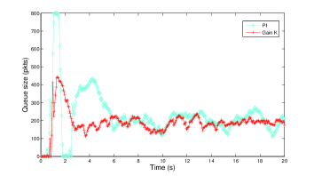
Figure 1: Time evolution of the queue length: comparison between PI and state feedback Gain K.

Simulations of perturbed system is reported in figures 2 and 3. In figure 2, we have increased the propagation delay by $20$ ms. Even if the system converges to a different reference point (slightly lower), the queue size is stable and quickly regulated.

Figure 2: Time evolution of the queue length for gain $K$ (calculated from DD robust stabilization)with a perturbation on the delay.

For more important pertubations (on the delay $R_{0}$ or number of sessions $N$), the system in closed-loop is still stable but the steady state changes since we converge to a new equilibrium point. In figure 3, a gain $K$ is calculated from DD robust stabilization with an external perturbation. The scenario is composed as follows: 7 additive sources (UDP protocol) send 1000 bytes packet length with a 1Mbytes/s throughput between $t=40s$ and $t=45s$. With the DD robust controller, the response is perturbed. The closed-loop system converges to the same reference, the queue size is stable and quickly regulated when the perturbation disappeared.

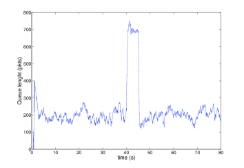
Figure 3: Time evolution of the queue length for gain $K$ (calculated from DD robust stabilization) with a perturbation as UDP traffic.

5 Conclusion

In this preliminary work, we have proposed the construction of robust AQMs for the congestion problem in communications networks. The developed AQMs have been established by using Lyapunov theory extended to delay systems and semi definite programming to solve the Linear Matrix Inequalities. Note that the proposed methods have been extended to the robust case where the delay in the loop is unknown. Finally, the AQMs have been validated using NS simulator.

References

- [1] S. Athuraliya, D. Lapsley, and S. Low. An enhanced random early marking algorithm for internet flow control. In IEEE INFOCOM, pages 1425–1434, December 2000.
- [2] S. Boyd, L. El Ghaoui, E. Feron, and V. Balakrishnan. Linear Matrix Inequalities in System and Control Theory. SIAM, Philadelphia, USA, 1994. in Studies in Applied Mathematics, vol.15.
- [3] J. Cleary, S. Donnely, I. Graham, A. McGregor, and M. Pearson. Design principles for accurate passive measurement. In PAM (Passive and Active Measurements) Workshop, Hamilton, New Zealand, pages 1–7, 2000.
- [4] K. Fall and K. Varadhan. The ns manual. notes and documentation on the software ns2-simulator. URL: www.isi.edu/nsnam/ns/.
- [5] V. Firoiu and M. Borden. A study of active queue management for congestion control. In IEEE INFOCOM, volume 3, pages 1435 – 1444, March 2000.
- [6] S. Floyd and V. Jacobson. Random early detection gateways for congestion avoidance. IEEE/ACM Transactions on Networking, 1:397–413, August 1993.
- [7] F. Gouaisbaut and D. Peaucelle. Delay-dependent stability analysis of linear time delay systems. In IFAC Workshop on Time Delay System (TDS’06), Aquila, Italy, July 2006.
- [8] F. Gouaisbaut and D. Peaucelle. A note on stability of time delay systems. In IFAC Symposium on Robust Control Design (ROCOND’06), Toulouse, France, July 2006.
- [9] K. Gu, V. L. Kharitonov, and J. Chen. Stability of Time-Delay Systems. Birkhäuser Boston, 2003. Control engineering.
- [10] C. V. Hollot, V. Misra, D Towsley, and W. Gong. Analysis and design of controllers for aqm routers supporting tcp flows. IEEE Trans. on Automat. Control, 47:945–959, June 2002.
- [11] K. B. Kim. Design of feedback controls supporting tcp based on the state space approach. In IEEE TAC, volume 51 (7), July 2006.
- [12] S. Kunniyur and R. Srikant. Analysis and design of an adaptive virtual queue (avq) algorithm for active queue management. In SIGCOMM’01, pages 123–134, San Diego, CA, USA, aug 2001.
- [13] Y. Labit, P. Owezarski, and N. Larrieu. Evaluation of active measurement tools for bandwidth estimation in real environment. In 3rd IEEE/IFIP Workshop on End-to-End Monitoring Techniques and Services (E2EMON’05), Nice (France), pages 71–85, May 2005.
- [14] L. Le, J. Aikat, K. Jeffay, and F. Donelson Smith. The effects of active queue management on web performance. In SIGCOMM, pages 265–276, August 2003.
- [15] H. S. Low, F. Paganini, and J.C. Doyle. Internet Congestion Control, volume 22, pages 28–43. IEEE Control Systems Magazine, Feb 2002.
- [16] W. Michiels, D. Melchior-Aguilar, and S.I. Niculescu. Stability analysis of some classes of tcp/aqm networks. In International Journal of Control, volume 79 (9), pages 1136–1144, September 2006.
- [17] V. Misra, W. Gong, and D Towsley. Fluid-based analysis of a network of aqm routers supporting tcp flows with an application to red. In SIGCOMM, pages 151–160, August 2000.
- [18] A. Papachristodoulou. Global stability of a tcp/aqm protocol for arbitrary networks with delay. In IEEE CDC 2004, pages 1029–1034, December 2004.
- [19] R.S. Prasad, M. Murray, C. Dovrolis, and K. Claffy. Bandwidth estimation:metrics, measurement techniques, and tools. In IEEE Network Magazine, 2003.
- [20] P. F. Quet and H. Özbay. On the design of aqm supporting tcp flows using robust control theory. IEEE Trans. on Automat. Control, 49:1031–1036, June 2004.
- [21] S. Ryu, C. Rump, and C. Qiao. Advances in active queue management (aqm) based tcp congestion control. Telecommunication Systems, 4:317–351, 2004.
- [22] R. Skelton, T. Iwazaki, and K. Grigoriadis. A unified algebric approach to linear control design. Taylor and Francis series in systems and control, 1998.
- [23] R. Srikant. The Mathematics of Internet Congestion Control. Birkhauser, 2004.
- [24] D. Wang and C. V. Hollot. Robust analysis and design of controllers for a single tcp flow. In IEEE International Conference on Communication Technology (ICCT), volume 1, pages 276–280, April 2003.