Blue luminescence of SrTiO₃ under intense optical excitation

Abstract

The blue-green photoluminescence emitted by pure and electron-doped strontium titanate under intense pulsed near-ultraviolet excitation is studied experimentally, as a function of excitation intensity and temperature. Both emission spectra and time-resolved decays of the emission are measured and analyzed in the framework of simple phenomenological models. We find an interesting blue-to-green transition occurring for increasing temperatures in pure samples, which is instead absent in doped materials. The luminescence yield and decay rate measured as a function of temperature can be modeled well as standard activated behaviors. The leading electron-hole recombination process taking place in the initial decay is established to be second-order, or bimolecular, in contrast to recent reports favoring a third-order interpretation as an Auger process. The temporal decay of the luminescence can be described well by a model based on two interacting populations of excitations, respectively identified with interacting defect-trapped (possibly forming excitons) and mobile charges. Finally, from the measured doping and sample dependence of the luminescence yield, we conclude that the radiative centers responsible for the luminescence are probably intrinsic structural defects other than bulk oxygen vacancies.

I Introduction

Strontium titanate, or SrTiO₃ (STO), is among the most widely investigated perovskite oxides, owing both to its potential for novel electronic applications and to its widespread use as a substrate for the epitaxial growth of strongly-correlated electronic materials, such as superconducting cuprates or colossal-magnetoresistive manganites. Recently, the puzzling transport properties of its interface with other insulating oxides have also attracted much interest.Huijben et al. (2009); Savoia et al. (2009) Despite this large effort, many properties of this material still await complete clarification.

Intrinsic STO is a band insulator, characterized by a huge static dielectric constant resulting from the rather soft bonding of the small Ti⁴⁺ ion to the surrounding octahedral O^2- cage. Its conduction band (CB) is composed of states having mainly Ti 3d t_2g character, while its valence band (VB) has dominantly O 2p character, with an upper edge located away from the $\Gamma$ point in the Brillouin zone.van Benthem et al. (2001) This results in an indirect gap of 3.2-3.3 eV, while the direct (optical) gap is 3.4-3.7 eV, with a non negligible sample and temperature dependence.van Benthem et al. (2001); Capizzi and Frova (1970) Upon $n$-type doping, generally achieved either by introducing O vacancies or by chemical substitution (e.g., La³⁺ for Sr²⁺ or Nb⁵⁺ for Ti⁴⁺), STO becomes a conductor with a relatively large low-temperature mobility.Frederikse and Hosler (1967); Kéroack et al. (1984) In this regime, it is known that the charge carriers are dressed by the interaction with the lattice and seem to behave mainly as large polarons, although with several nonstandard features.Kéroack et al. (1984); Eagles et al. (1996); van Mechelen et al. (2008); Ishida et al. (2008) When intrinsic STO is irradiated with ultraviolet (UV) light, photogenerated electrons and holes (e,h) appear to both contribute to the material photoconductivity.Itoh et al. (2005) Theoretical calculations would also indicate that holes in pure STO are not strongly coupled to phonons and keep their bare mass.Stashans (2001)

The photoluminescence (PL) properties of STO are possibly even more puzzling and controversial than its transport ones. The greenish luminescence (GL) having a maximum at 2.2-2.4 eV of photon energy (wavelength $\lambda\approx 500$ nm) that is emitted by pure STO at low temperature under exposure to UV or X-ray radiation has been known since a long time,Grabner (1969); Feng (1982); Aguilar and Agullo-Lopez (1982) and is generally ascribed to the decay of intrinsic self-trapped excitons (STE).Leonelli and Brebner (1986); Hasegawa et al. (2000); Deguchi et al. (2008); Qiu et al. (2008) A STE can be roughly depicted as a tightly bound state of a hole and a Ti³⁺ polaron.Prócel et al. (2003); Eglitis et al. (2003) However, this purely intrinsic scenario has been recently called into question by Mochizuki et al.,Mochizuki et al. (2005, 2006) who argued for a crucial role of defects and possibly of surfaces in this GL emission.

Only recently, another photoluminescence emission taking place in the blue (BL), with its maximum at 2.8-2.9 eV ($\lambda\approx 430$ nm), was reported for STO at room temperature.Mochizuki et al. (2005); Kan et al. (2005) This BL emission, potentially useful for optoelectronic applications, is well visible both in intrinsic samples at sufficiently high excitation intensitiesMochizuki et al. (2005) and in suitably $n$-doped samples, in the latter case at much lower excitation intensities.Kan et al. (2005, 2006) A similar blue luminescence was also observed for intense electron-beam excitation.Grigorjeva et al. (2004); Zhang et al. (2008) At low temperatures, the blue emission is accompanied by a spectrally-narrow near-UV emission (UVL) located at 3.2 eV ($\lambda\approx 390$ nm), i.e. at band edge.Mochizuki et al. (2005); Kan et al. (2005, 2006) Moreover, in some cases the BL may also be accompanied by a long green “tail” covering a spectrum similar to the GL discussed above, but still visible at room temperature.Mochizuki et al. (2005); h. Li et al. (2007) It is not clear what determines the appearance of this high temperature GL component, but surface state of oxidation seems to play an important role.Mochizuki et al. (2005) This GL is clearly visible at high excitation intensities.Rubano et al. (2007, 2008)

The underlying nature of this room temperature BL is still far from clear. Although the BL yield is enhanced by $n$-doping, its spectrum looks nearly identical for different kinds of doping as well as for intrinsic samples under intense excitation (but this is only true at room temperature, as we will see below),Mochizuki et al. (2005); Kan et al. (2006); Rubano et al. (2008) thus pointing to a role of conduction band electrons rather than donor levels in the enhancement.Kan et al. (2006) When studied as a function of temperature, in contrast with the GL which vanishes quickly above 30-50 K, the BL exhibits a yield that is steadily increasing with temperature, reaching a maximum at about 160 K and then decreasing slowly (a faster decrease is however observed at temperatures substantially higher than room temperature, as we will see below).Mochizuki et al. (2005); Yamada et al. (2009) Studied as a function of the excitation fluence (for short laser pulse excitation), the BL yield shows no saturation up to very high fluences, in the mJ/cm² range, while the low-temperature GL has a much smaller saturation threshold.Mochizuki et al. (2005); Rubano et al. (2007) More precisely, a detailed recent study by Yasuda et al. has shown that in pure STO the BL yield is actually quadratic in the excitation pulse fluence up to about 1 mJ/cm².Yasuda and Kanemitsu (2008) Above this value there is initially a crossover to an approximately linear behavior and then at 30-40 mJ/cm² a full saturation.Mochizuki et al. (2005); Rubano et al. (2007); Yasuda and Kanemitsu (2008) A strong dependence of the BL spectrum and yield on a previous surface treatment with fluorhydric acid has been also reported,h. Li et al. (2007) possibly pointing to a role of the surface or of other crystal imperfections in the luminescence process, although these results could be also explained as resulting from a variation of the surface-induced fluorescence quenching, thus unrelated with the radiative process itself (in Ref. h. Li et al., 2007 the excitation wavelength was 325 nm, at which the penetration length in STO is of only few tens of nanometers, thus enhancing the role of the surface).

Even more intriguing is the PL dynamical behavior studied as a function of time following a very short pulse excitation. It is clearly established that the PL decay does not follow a simple exponential behavior. At low temperatures, the GL band is associated with a slow power-law decay, with a very strong temperature dependence, typical of an untrapping-rate-limited “bimolecular” dynamics.Leonelli and Brebner (1986); Hasegawa et al. (2000); Mochizuki et al. (2005) The BL dynamics has been studied in detail by us as a function of excitation energy (in a strong excitation regime), and we observed an interesting nonlinear dynamics, which can be modeled as a quite simple two-component decay.Rubano et al. (2007) One component seems to be exponential, or “unimolecular”, while the other one can be fitted well by a bimolecular power-law decay.Rubano et al. (2007) Although apparently similar to the bimolecular behavior of GL seen at low temperatures, the BL one is much faster (also at low temperatures) and hence must be ascribed to a different process.Mochizuki et al. (2005) The two dynamical components are present in the whole BL spectrum, including its green “tail”, apparently with no significant wavelength dependence.Rubano et al. (2007) Doped samples exhibit a similar two-component dynamics as pure ones and, at high excitation fluences, also similar decay times and yields, with no evident doping-induced enhancement.Rubano et al. (2008) However, as shown by Yasuda et al., at smaller excitation intensities both the overall luminescence yield and the exponential decay rate of the unimolecular component are found to be strongly dependent on the dopant concentration.Yasuda and Kanemitsu (2008) In the same paper, in contrast with our previous results, Yasuda et al. claim that the two-component decay is actually best described by an Auger trimolecular process acting together with the unimolecular one, thus leaving the issue of the leading recombination process governing the PL decay undecided. Properly assessing the strength of the Auger recombination may be important for proposed applications of STO in opto-thermionic refrigeration.li Zhang et al. (2009) We will come back to this issue below.

In this work, we investigate further the physics underlying the blue luminescence of STO by analyzing the PL spectra and temporal decays, for both intrinsic and doped samples, as a function of excitation energy and temperature. The temperatures of our measurements are high enough to make the activated luminescence quenching evident. Moreover, we compare in detail the predictions of different models for the PL dynamical behavior, in order to establish the nature of the recombination processes involved in the decay and to shed light on the underlying electronic mechanisms.

This paper is structured as follows. Section 2 describes the experimental procedures. The wavelength-resolved studies as a function of excitation energy and temperature are reported and analyzed, within a simple model, in Sec. 3. The corresponding time-resolved studies are then reported in Sec. 4, together with a first phenomenological modeling. In Sec. 5 we tackle the question of a more detailed modeling of the dynamical behavior. The final Section 6 includes a discussion of the physics underlying the dynamical models used for interpreting the PL decay and a summary of our main results.

II Experiments

The samples used in this work were of the following three kinds: (i) five stoichiometric intrinsic (100)-oriented STO single crystals (I-STO), $1\times 5\times 5$ mm³ in size, produced by four different companies (SurfaceNet GmbH, CrysTec GmbH, Crystal GmbH, eSCeTe B.V.) by the flame-fusion Verneuil method, with specified impurity levels all below 150 ppm, and used as received; (ii) two samples of Nb-doped STO crystals (N-STO), with a Nb molar concentration of 0.2%, and having the same orientation and geometry as the I-STO samples; (iii) one sample doped with oxygen vacancies (O-STO), obtained from a pure sample by annealing for 1 h at 950^∘C and 10^-9 mbar (base pressure 10^-11 mbar). While I-STO samples look transparent and are verified to be good insulators, both N-STO and O-STO samples look black/dark-blue opaque and are conducting. In O-STO, from resistivity measurements performed on a thin film annealed by the same procedure, we estimate an induced carrier density of $3\times 10^{17}$ cm^-3, or about 0.002%, rather small but still much higher than typical residual oxygen vacancy concentrations in nominally stoichiometric samples.Rubano et al. (2008) I-STO and N-STO samples did not show aging or hysteretic behavior due to oxygen exchange with atmosphere, as we checked by repeated measurements. Instead, O-STO samples turned transparent again when heated above 250 ^∘C in air, clearly showing re-oxidation of the vacancies. For this reason, all our temperature behavior studies were limited to I-STO and N-STO samples. During measurement, the samples were held into a thermostat for temperature control to within 0.1 K (with an accuracy within few K). The temperature was scanned between 300 K and 900 K.

In all our experiments, the excitation was induced by 3.49 eV UV photons ($\lambda=355$ nm) in 25-ps-long laser pulses at 10 Hz repetition rate focused to a gaussian spot having a radius of $1.2\pm 0.1$ mm at $1/e^{2}$ of maximum. The energy per pulse was varied from 40 $\mu$J to 2 mJ, corresponding to an excitation fluence $U$ ranging from a minimum of 2 to a maximum of 100 mJ/cm² (value at the spot center, corresponding to twice the spatial-average value). This goes up to much higher values than those investigated by others, including Mochizuki et al. (up to 14 mJ/cm²)Mochizuki et al. (2005) and Yasuda et al. (up to 10 mJ/cm²)Yasuda and Kanemitsu (2008). For our highest fluence of 100 mJ/cm², taking into account the 25% reflection and assuming an optical penetration length of about 1 ${\mu}m$,Capizzi and Frova (1970) we estimate a peak density of photogenerated e-h pairs as high as $1.2\times 10^{21}$ cm^-3. This corresponds to a fluence-to-density conversion factor (FDCF) $\alpha=1.2\times 10^{22}$ cm^-1/J. It must be noted, however, that the UV penetration length is highly uncertain, as different samples have shown fairly different absorption edges in previous reports. We stress that, despite our large excitation fluences, no visible photoinduced damage of the sample surfaces was induced during our experiments and we never observed irreversible variations of the signal as a function of excitation intensity.

The luminescence emitted from the sample was collected by a lens system imaging the illuminated sample spot onto the detector head, after blocking the (much stronger) elastic scattering by a long-pass filter with a cutoff wavelength of 375 nm. When recording the luminescence spectra, for detection we used a grating-monochromator and a photomultiplier and integrated the signal in time (with a 50 ns time gate). In time-resolved measurements, the luminescence was instead detected with a photodiode (PD) having a rise-time of about 150 ps. In time-resolved experiments the entire luminescence spectrum was integrated. The PD signal was acquired by a 20 Gsample/s digital oscilloscope having an analog bandwidth of 5 GHz. The response function $r(t)$ of this apparatus was acquired by measuring the signal given by the elastic scattering of the excitation pulse (taken after removing the long-pass filter).

III Measurement results: spectra

Figure 1: (Color online) Photoluminescence spectra from I-STO (panels a and b) and N-STO (panels c and d) samples at various temperatures and at an excitation fluence of 2.2 mJ/cm² (panels a and c) or 22 mJ/cm² (panels b and d). Labels GL, BL, and VL (green, blue, and violet luminescence) in panel (a) mark the peaks of the three separate luminescence bands that can be singled out in our spectra. A blue-to-green spectral transition (a red-shift of the peak) of the photoluminescence is seen in the I-STO spectra, while it is absent in the N-STO doped samples. The lines in panel (b) are best-fit curves based on our theory. The lines in the other panels are guides to the eye.

The data shown in Fig. 1 refer to a typical I-STO (panels a and b) and a typical N-STO sample (panels c and d), respectively under 2.2 (panels a and c) and 22 mJ/cm² (panels b and d) excitation fluences, respectively. It is seen that the overall shape of all spectra is asymmetrical, with both GL and BL emissions present and clearly distinguishable at all temperatures, in spite of a substantial overlap. At a closer inspection, an additional spectral contribution apparently located at about 3.0 eV ($\lambda\approx 400$ nm, in the violet), henceforth called VL (see panel a), can be singled out, particularly in I-STO samples (it is however possible that this emission is actually the same as the UVL band mentioned in the Introduction, after a reshaping due to the detection-line long-pass filter used in our setup). This VL appears as a small shoulder in the lower temperature measurements, while it is more clearly separated, although strongly depressed, at higher temperatures. Our spectra are qualitatively consistent with literature data. Three distinct emissions with similar spectral position were reported in Ref. Mochizuki et al., 2005, though at lower temperature. The spectrum of La-doped STO reported in Ref. Kan et al., 2006 closely resembles that of our N-STO samples at 300 K. However, compared to previous data, ours seem to show a comparatively higher yield in the GL region. In all samples the GL contribution appears to increase more weakly than the BL one for an increasing excitation intensity, as can be seen in Fig. 1 by comparing panels (a) with (b) and (c) with (d). Therefore, the GL emission is probably more saturated than the BL one, pointing to the presence of different classes of emitters as responsible for the two bands.

As a function of temperature $T$, the most striking feature seen in the PL spectra is a strong red-shift of the BL maximum occurring for increasing $T$ in I-STO samples. I-STO samples at high temperature emit almost exclusively in the green, with only a small residual emission in the blue (which we ascribe to the VL band). This blue-to-green thermal transition of the luminescence can be clearly seen even with the naked eye. The fact that this shift does not occur (or is very small) in N-STO doped samples, makes the spectra of I-STO and N-STO samples become very different at high temperatures. This is an important observation, as it is the first clear qualitative difference seen in the luminescence spectra of doped samples as compared to pure ones. In contrast to what stated before,Kan et al. (2006); Yasuda and Kanemitsu (2008) this shows that the role of doping is not limited to introducing additional charge carriers in the system, but somehow affects also the properties of the radiative and/or non-radiative recombination centers.

In order to analyze the data quantitatively, we will refer to a specific model for the spectral shape $I(\omega)$ of each component of the luminescence spectrum (GL, BL, and VL), treating them as independent. As previously stated, the low-temperature GL was interpreted in a quantitative way by Leonelli and Brebner in terms of the annihilation of self-trapped excitons of given energy $E_{0}$.Leonelli and Brebner (1986) In this picture, the broadening of the band is due to the random emission of several optical phonons, each of energy $\hbar\Omega\approx 90$ meV, giving rise to the following expression:

$$I(\omega)=I_{0}e^{-S_{0}}\sum_{n=0}^{\infty}\frac{S_{0}^{n}\Gamma/(2\pi n!)}{(E_{0}-\hbar\omega-n\hbar\Omega)^{2}+(\Gamma/2)^{2}},$$ (1)

whose key parameter is the Huang-Rhys factor $S_{0}$, related to the strength of the electron-lattice interaction and fixing the average number of emitted phonons per recombination. $\Gamma$ is the width of the band associated with a given $n$-phonon process, taken to be Lorentzian. Although devised for self-trapped excitons, Eq. (1) applies equally well to the case of defect-assisted recombinations – in which defects mediate the coupling of the electronic excitation to the lattice – , so it may be actually considered as a semi-phenomenological model that can describe different microscopic scenarios. Leonelli and Brebner found that a value as high as $S_{0}=5.7$ produced a nice fit to the data, meaning that the maximum of intensity at 2.4 eV is well shifted with respect to the intrinsic exciton energy, taken at $E_{0}\approx 2.9$ eV. We plotted the $I(\omega)$ resulting from Eq. (1), keeping the same quoted values of the parameters $S_{0}$ and $E_{0}$ and assuming a broadening factor $\Gamma=0.12$ eV: even with no adjustable parameters (except for the overall amplitude scale), we could describe in this way quite accurately the GL band shape in the region where it is well separated from the other bands (see, e.g., the highest temperature spectrum in Fig. 1b). Hence, we assumed that the GL band keeps the same form in all spectra, except for a temperature dependent scale factor, and turned to the problem of the BL and VL bands. Tentatively, given its general applicability, we used Eq. (1) also for these bands, and after suitable adjusting of the parameters $E_{0}$ and $S_{0}$ we could achieve a satisfactory fit of all data. The phonon energy $\hbar\Omega$ and the irrelevant broadening factor $\Gamma$ were always kept fixed at the values 88 meV and 0.12 meV, respectively, without any attempt of optimization. The optimal values of the characteristic energies and of the Huang-Rhys factors for the GL, BL and VL components were determined by a global fit procedure as $\simeq$2.9 eV, $\simeq$2.9 eV, $\simeq$3.0 eV, and $\simeq$5.5, $\simeq$1, $\simeq$1, respectively, independently of fluence and temperature, and allowing for only a slight sample dependence. In addition, we used as free fit parameters the respective amplitudes $I_{0}$ of the three bands at each temperature. Typical results for pure and doped samples are reported in Fig. 2. As a last step, we observed that allowing for a slight decrease of the characteristic energy of the VL contribution for increasing temperature (in any case below 0.1 eV) the fit was further improved. This shift can be probably associated with the known temperature dependence of the STO gap.Blazey (1971) An example of the fit results is given in Fig. 1b. The overall fit quality is as good in all I-STO and N-STO investigated samples.

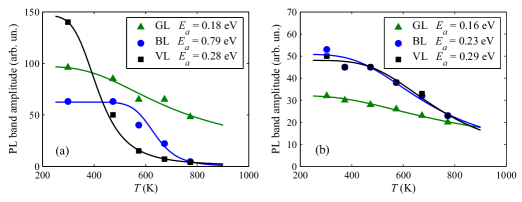
Figure 2: (Color online) Temperature behavior of the amplitudes of the three spectral bands GL (triangles), BL (circles), and VL (squares) as seen in the I-STO (panel a) and N-STO (panel b) photoluminescence. The excitation fluence was 2.2 mJ/cm². Solid lines are best fits based on Eq. (2); the resulting activation energies are reported in the legend. The case of high excitation fluence (22 mJ/cm²) gives similar results, except for a slightly smaller activation energy of the VL component ($\approx 0.2$ eV instead of $\approx 0.3$ eV).

Figure 2a shows that the blue-to-green transition of I-STO samples can be explained as a thermal quenching of the VL and BL components occurring at lower temperatures than for the GL one. This is not the case of N-STO samples, for which the three amplitudes have a more similar behavior with temperature, as shown in Fig. 2b. The thermal quenching of the PL amplitudes $I_{0}(T)$ can be approximately modeled by the following standard Arrhenius activation law:

$$I_{0}(T)\propto\tau(T)\propto\left[a+be^{-E_{a}/(k_{b}T)}\right]^{-1},$$ (2)

where $\tau$ is the characteristic PL decay time, $E_{a}$ an activation energy giving the potential barrier of the competing non-radiative relaxation channels, $k_{b}$ the Boltzmann constant and $a,b$ are constants that give the relative weight of the temperature independent (typically radiative) and thermally activated (typically non-radiative) contributions to the decay, respectively. The best fit results based on Eq. (2) are also shown in Fig. 2. The corresponding activation energies are all of the order of tenths of eV, with somewhat smaller values for GL (0.16-0.18 eV), and slightly larger for BL and VL (0.23-0.29 eV), with the exception of the BL in I-STO, which is found to be about 0.8 eV. According to these best-fit results, the stronger thermal quenching of the BL and VL bands compared to GL is not associated to a smaller activation energy (it is actually larger), but to a relatively larger weight of the non-radiative channels with respect to the radiative ones.

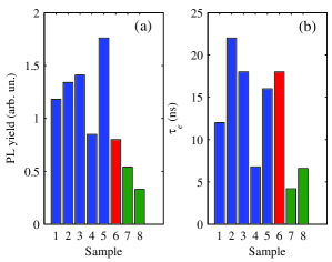
Figure 3: (Color online) Histogram of the PL yield (panel a) and PL-tail exponential decay time $\tau_{e}$ (panel b), for different samples at room temperature. Samples 1-5 are I-STO (blue online), sample 6 is O-STO (red online) and samples 7-8 are N-STO (green online).

Finally, the spectrally-integrated PL yield at a pump fluence of 2.2 mJ/cm² as a function of the sample at room temperature is shown in Fig. 3a. The most important things to notice here are the following: (i) there is a significant sample-to-sample dependence of the yield in nominally identical I-STO samples; (ii) doped O-STO and N-STO samples do not show any enhanced yield, despite the presence of many additional donor defects. We will discuss these findings in Sec. 6.

IV Measurements results: temporal decays

A typical set of PL temporal decays measured from a I-STO sample for various excitation pulse fluences $U$ is shown in Figs. 4-5. The case of N-STO is very similar (an example is reported in Fig. 2 of Ref. Rubano et al., 2008).

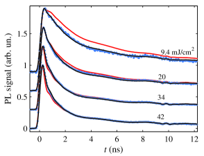
Figure 4: (Color online) Time decay of the PL signal of a I-STO sample following its excitation by a UV picosecond pulse, for different excitation fluences, at room temperature. Data are shown as gray dots (blue online). The solid lines are the result of a global best fit based on our models (including a final convolution with the measured instrumental response time $r(t)$). The black line is based on the C2PUBv1 bimolecular model and the gray line (red online) is based on the 1PUT trimolecular model. Data and curves referring to different fluence values are vertically shifted for clarity.

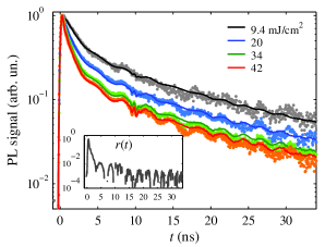
Figure 5: (Color online) Time decays of the PL signal of a I-STO sample at room temperature, for different excitation fluences, shown here in semi-logarithmic scale to highlight the exponential PL tail. Data are shown as dots, while the solid lines are the result of a global best fit based on the C2PUBv1 model. The wiggles seen in the tail for both data and model predictions are due to the detection-system response function $r(t)$, which is shown in the inset (inset axes labels and units are the same as for main panel).

As already noted in our previous works and confirmed by Yasuda et al.,Rubano et al. (2007, 2008); Yasuda and Kanemitsu (2008) the PL initial decay becomes faster for higher excitation energies, while the final part of the decay (the “tail”) varies only in its amplitude, relative to the peak, but not in its rate. One can therefore phenomenologically single-out two distinct regimes: the initial fast decay, with an excitation-dependent characteristic decay time, and the final tail, with a well defined, excitation-independent, exponential decay time $\tau_{e}$. In I-STO, the fast decay is typically in the range 1-2 ns (for our excitation fluences) and is only weakly sample dependent, while the slow tail time constant ranges from 6 to 23 ns, depending on the sample, as shown in Fig. 3b. In N-STO the fast decay rate is of the same order as in I-STO, while the exponential decay becomes somewhat faster ($\tau_{e}\approx 5$ ns), as an effect of doping.Yasuda and Kanemitsu (2008)

In Figs. 4-5 the decay signals are normalized to their maximum, for clarity. However, also the PL signal amplitude varies strongly with the excitation intensity. More precisely, as mentioned in the Introduction, we observed an approximately linear dependence of the time-integrated PL signal, i.e. of the overall PL yield, on excitation fluence up to 30-40 mJ/cm², while for even higher fluences we find a saturation (see Fig. 2 of Ref. Rubano et al., 2007 and Fig. 3 of Ref. Rubano et al., 2008). The PL signal maximum typically shows a mixed linear-quadratic behavior with excitation fluence, with a relatively large scatter of the data, for reasons which we have not yet identified. The exact threshold for saturation is also sample dependent, pointing again to an important role of the defects in the PL radiative channels. Moreover, the linear yield behavior we find in our data is actually already a partly saturated one, as for lower excitation fluences a quadratic behavior is observed instead.Yasuda and Kanemitsu (2008)

To specify a characteristic experimental decay time for each given PL signal, we use its full-width-at-$1/e$-of-the-maximum (FW$1/e$M) time $t_{1/e}$. Equivalently, its inverse $t_{1/e}^{-1}$ provides a characteristic decay rate. The measured decay rates $t_{1/e}^{-1}$ versus excitation fluence $U$, for different temperatures, in a I-STO sample, are shown in Fig. 6. N-STO samples give very similar results.

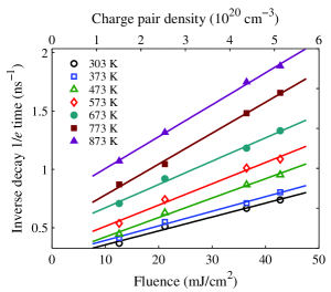
Figure 6: (Color online) Experimental decay rates as a function of excitation fluence and temperature, for a I-STO sample. The decay rate is here defined as the inverse of the FW$1/e$M decay time $t_{1/e}$. The upper $x$ axis gives our estimate of the density of photoinduced electron-hole pairs after excitation. The lines are linear best fits of the fluence dependence.

In the investigated range, this decay rate shows an approximate linear dependence on the excitation fluence, as shown in the figure. However, since the measured decay times $t_{1/e}$ are close to the characteristic response time of our detection apparatus, these raw data for $t_{1/e}$ are significantly larger than the actual decay times of the luminescence. To take care of this, in principle we should deconvolve the measured decay signal and the response function of our setup. However, the numerical deconvolution of noisy data is known to be problematic, so that, following the standard procedure, we used the inverse approach. Given a theoretical model $I(t)$ for the PL decay containing the characteristic times to be determined as adjustable parameters, we first convolve it with the measured response function $r(t)$, thus obtaining a predicted signal $S(t)=(r*I)(t)$. The latter is then compared with the measured signal, thus finding the best-fit values of the adjustable parameters. In this way, the best-fit values of the characteristic decay times appearing as parameters in the model function $I(t)$ will correspond to actual PL decay times, without significant distortions due to the instrumental response function. The final time-resolution that can be achieved with this approach is limited only by the signal-to-noise ratio of our data (typically $10^{2}-10^{3}$). In this Section, we wish to analyze the data without relying on too specific physical assumptions: ideally, we would like to adopt a model-independent description, postponing the analysis of specific models to the following Section. Therefore, we adopt here the “phenomenological” model already used in Ref. Rubano et al., 2007 (corresponding to the 2PUB considered in next Section). According to this model, the PL intensity as a function of time is given by the sum of a pure unimolecular exponential decay with time constant $\tau_{1}$ and a pure bimolecular decay with excitation-dependent time constant $\tau_{2}=1/(\gamma\alpha_{2}U)$, where $\gamma$ and $\alpha_{2}$ are constants.Rubano et al. (2007) The fast FW$1/e$M time $t_{1/e}$ will be approximately proportional to the value of $\tau_{2}$. For each given sample and temperature, we may assign a typical value to the time constant $\tau_{2}$ by fixing a reference excitation fluence $U_{1}$ at which it must be evaluated. We choose here a value for $U_{1}$ that is in the order of our experimental range, i.e. $U_{1}=10$ mJ/cm².

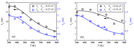
Figure 7: (Color online) Characteristic PL decay times $\tau_{1}=\tau_{e}$ (squares) and $\tau_{2}$ (circles), the latter at the reference fluence of 10 mJ/cm², versus temperature $T$, for a I-STO sample (panel a) and a N-STO sample (panel b). The lines are best fits based on the activated behavior given by Eq. (2). The resulting activation energies are given in the legend.

The best-fit values of the exponential slower decay time $\tau_{1}=\tau_{e}$ and of the faster initial decay time $\tau_{2}$ (at the reference fluence of 10 mJ/cm²) for a I-STO and a N-STO samples are shown in Fig. 7 (the fit procedure is described in more detail in the next Section). As in the case of the PL spectral amplitudes, all decay time temperature behaviors can be fitted fairly well by the Arrhenius law given by Eq. (2). The resulting activation energies are given in the figure legend and are in the range $0.2-0.3$ eV, of the same order as those obtained from the behavior of the PL band amplitudes.

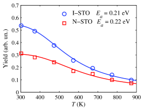
Figure 8: (Color online) Photoluminescence yield, computed from the time-integral of the decay signal, as a function of temperature, for a I-STO and a N-STO samples. Solid lines are best fits based on the activated behavior given by Eq. (2). The resulting activation energies are given in the legend.

To conclude this Section, we report in Fig. 8 the measured temperature behavior of the PL yields obtained from the time integral of the decays, together with the usual activation-law best-fits. The resulting activation energies are again roughly consistent with the dynamical ones and with the spectral amplitude ones. No significant dependence on doping is found in this case.

V Modeling the temporal decay

Although it is firmly established that the initial decay rate of the PL at sufficiently high excitation intensities behaves nonlinearly,Rubano et al. (2007, 2008); Yasuda and Kanemitsu (2008) the exact decay law and the underlying microscopic relaxation mechanisms are currently controversial, as we mentioned in the Introduction. In this Section we introduce and compare several different models for the PL decay, listed in Table I, aiming at identifying the most effective one in describing our data, which can in turn offer indications about the underlying microscopic physics (to be discussed in the next Section). In particular, we are especially interested in assessing the order of the leading recombination mechanism, e.g., bimolecular versus trimolecular.

Each tested model is labeled with a code (first column in Table I) which synthesizes the most important assumptions on which it is based: (i) the figure before the letter “P” gives the number of decaying electron populations considered in the model (either 1 or 2), with a “C” denoting the more specific case of coupled populations; (ii) the letters “U, B, T” stand respectively for unimolecular, bimolecular and trimolecular recombination mechanism (a unimolecular recombination process is taken to be present in all models); “v1” and “v2” denote different variants of the same basic model.

In this work, we adopted a “global fit” procedure, that is we fitted simultaneously all the decays measured for a given sample at a given temperature but for different values of the fluence $U$, for a single choice of the adjustable parameters. For each model and for all samples and temperatures, we have performed global best fits of the following two kinds: (i) “without the amplitudes”, i.e. on signals which had been previously normalized to their maximum; (ii) “with the amplitudes”. The reason for using both methods is that the PL decay amplitudes were usually subject to a significant scatter, not present in the decay functional form, and for the highest excitation fluences also to some degree of saturation, which may not be properly taken into account in our simple models. Therefore, approach (i) is more appropriate in order to focus on the capability of our models to predict the $U$-dependence of the PL decay functional form, and in particular of the PL decay rates, regardless of the amplitude behavior. Approach (ii) tests the models in their predictive power for both PL rates and amplitudes, but tends to weight more the amplitude behavior, as it gives the strongest data variations. All compared models have four adjustable parameters in approach (ii), while in approach (i) all models have three parameters except for one (C2PUBv1), which has four. For each approach, we quantified the performance of each model with the fit $\chi^{2}$ (normalized to the data variance, estimated using the measured noise before the excitation pulse), averaged over different samples and repeated measurements as specified in Table I.

Table 1: Different PL decay models tested in this work. The two best-fit values of $\chi^{2}$ reported in the last two columns are averaged over different samples and repeated measurements, after normalizing to the minimum $\chi^{2}$ value obtained among all models for each given sample/measurement (in order to weight all samples equally). The first $\chi^{2}$ (no ampl.) is computed for decays normalized to their maximum, so that the behavior of the decay amplitude with excitation fluence does not enter the fit and the model testing is focused on the decay rates. The second $\chi^{2}$ (with ampl.) is instead computed taking also the decay amplitudes into account. The reported differences are statistically highly significant (the formal likelihood ratio between the best model and the others is of thousands of orders of magnitude).

model code	rate equations	initial conditions	radiative term	$\chi^{2}$ no ampl.	$\chi^{2}$ with ampl.
1PUB	$dN/dt=-N/\tau_{1}-\gamma N^{2}$	$N(0)=\alpha U$	$I=Q\gamma N^{2}$	2.1	1.9
1PUT	$dN/dt=-N/\tau_{1}-C_{A}N^{3}$	same as above	$I=Q\gamma N^{2}$	3.2	1.8
2PUB	$\begin{array}[]{l}dN_{1}/dt=-N_{1}/\tau_{1}\\ dN_{2}/dt=-\gamma N_{2}^{2}\end{array}$	$\begin{array}[]{l}N_{1}(0)=\alpha_{1}U\\ N_{2}(0)=\alpha_{2}U\end{array}$	$I=Q_{1}N_{1}/\tau_{1}+Q_{2}\gamma N_{2}^{2}$	2.2	1.7
2PUT	$\begin{array}[]{l}dN_{1}/dt=-N_{1}/\tau_{1}\\ dN_{2}/dt=-C_{A}N_{2}^{3}\end{array}$	same as above	$I=Q_{1}N_{1}/\tau_{1}+Q_{2}\gamma N_{2}^{2}$	3.1	1.7
C2PUBv1	$\begin{array}[]{l}dN_{1}/dt=-N_{1}/\tau_{1}-\gamma_{1}N_{1}N_{2}\\ dN_{2}/dt=-\gamma_{2}N_{2}^{2}\end{array}$	same as above	$I=Q\left|dN_{1}/dt\right|$	1.0	1.7
C2PUBv2	same as above	$\begin{array}[]{l}N_{1}(0)=\alpha_{0}+\alpha_{1}U\\ N_{2}(0)=\alpha_{2}U\end{array}$	$I=Q\gamma_{1}N_{1}N_{2}$	1.3	1.1

The first two models in Table I (1PUB and 1PUT) are based on the assumption that a single-population density $N(t)$ of decaying electrons and holes (balanced in number) suffices for capturing the recombination dynamics revealed by the PL decay. Many past analyses of picosecond-laser-induced PL temporal decays in semiconductors (see, e.g., Refs. Zarrabi et al., 1985; Landsberg, 1987; Linnros, 1998), as well as the recent work of Yasuda et al. on the STO,Yasuda and Kanemitsu (2008) interpret the PL decay by a similar single population model. While the unimolecular and bimolecular terms are fairly common in solid state luminescence, the appearance of a third-order trimolecular term, typically ascribed to Auger processes involving two electrons and a hole or two holes and an electron, is only seen at very high excitation densities in indirect band-gap materials. In principle, it is quite reasonable to expect this behavior in the case of STO, and indeed the 1PUT model is that assumed in Ref. Yasuda and Kanemitsu, 2008. However, we find that the 1PUT model is very ineffective in describing our data. An example of the unsatisfactory results of a global fit based on the 1PUT model is shown in Fig. 4 (gray lines, red online), while the average best-fit $\chi^{2}$ values relative to the best-performing models are reported in Table I.

We stress that by using a global (simultaneous) fit on all the decays obtained at different excitation energies $U$, we have put the models to the test not only on their capability to predict the single-decay functional form, but also on their capability to predict the overall dependence of this functional form on the excitation fluence $U$. This dependence is very sensitive to the order of the highest nonlinear term in the decay equations and therefore matching this dependence provides a much stricter test than matching the single-decay behavior. More precisely, the initial rate of decay taking place shortly after excitation is predicted to depend much more strongly on the excitation fluence $U$ for the 1PUT model than for a second-order model, such as 1PUB (see Table I). Indeed, assuming that the PL signal is generated by a given power $p$ of the population density, $I(t)\propto N^{p}(t)$ (e.g., $p=2$ for a bimolecular radiative recombination), the initial logarithmic decay rate for a single population model including both bimolecular and trimolecular terms is given by

$$\left.-\frac{d\ln I}{dt}\right|_{t=0^{+}}=\left.-\frac{p}{N}\frac{dN}{dt}\right|_{t=0^{+}}$$

$$=p\left[\frac{1}{\tau_{1}}+\gamma N(0^{+})+C_{A}N^{2}(0^{+})\right]$$ (3)

$$=p\left(\frac{1}{\tau_{1}}+\gamma\alpha U+C_{A}\alpha^{2}U^{2}\right)$$

Thus, for the 1PUT model one would expect a quadratic dependence of this initial decay rate on excitation fluence $U$, while for a second-order (bimolecular) model, having $C_{A}\approx 0$, one expects a linear dependence. This initial decay rate is well estimated by the inverse FW$1/e$M time $t_{1/e}^{-1}$. We indeed find a linear behavior, as shown in Fig. 6, and this supports a bimolecular model.

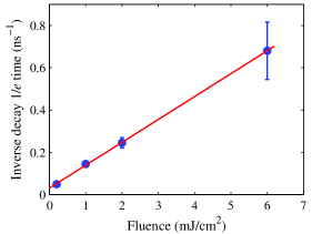
Figure 9: (Color online) Inverse decay times versus excitation fluence for the four PL decay curves reported in Fig. 1 of Ref. Yasuda and Kanemitsu, 2008. The times have been estimated graphically, from the initial decay slope in the semi-logarithmic chart. The line (red online) is a linear best-fit. The good linearity of the decay rates vs fluence confirms a bimolecular behavior for the initial fast decay.

To investigate also the hypothesis of a crossover from a trimolecular behavior taking place for the lower fluence range studied by Yasuda et al. ($0-10$ mJ/cm²) to a bimolecular one in our higher range of fluences ($10-50$ mJ/cm²), we graphically extracted from Fig. 1 of Ref. Yasuda and Kanemitsu, 2008 the initial logarithmic slope of the four reported decays. These values are plotted in Fig. 9 versus the excitation fluence, showing that the behavior is again perfectly linear in $U$ as expected from a bimolecular model (not necessarily a single-population model), and hence not consistent with a third-order model such as 1PUT. We note that the fluence dependence of the measured decay rates can be altered by the finite response function of the apparatus. The data from Ref. Yasuda and Kanemitsu, 2008 were taken with a streak camera, which typically has a very fast response in the picosecond range, so that they should not be affected by this problem. Our data are instead affected by the slower response time of our equipment. Nonetheless, even after convolution with the response function, the 1PUT third-order model predicts a stronger dependence of the initial decay rate on the excitation fluence than what seen in our data, as shown already in Fig. 4, and more explicitly in Fig. 10.

In synthesis, we can conclude that the initial faster decay is a second-order, or bimolecular, recombination process and no significant trimolecular effect is detected in our data. We note however that even at fluences much smaller than ours, indirect semiconductors usually exhibit a strong Auger-like third-order decay.Zarrabi et al. (1985); Linnros (1998); Landsberg (1987) Presumably, third-order Auger interactions are depressed in STO by its relatively large band-gapMassé et al. (2007) and high dielectric constant, while bimolecular recombinations might be favored by its comparatively large density of intragap trapping states and by its stronger electron-phonon interactions.

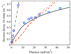
Figure 10: (Color online) Inverse decay rates versus fluence as measured for a I-STO sample (squares) and as predicted by different models (lines), after a global best fit on the measured decays. Besides ours, the Yasuda et al. data already given in Fig. 9) are also plotted (circles). The two sets of data do not merge into a single smooth behavior because of the much slower response of our apparatus as compared to that used by Yasuda et al. in Ref. Yasuda and Kanemitsu, 2008. The predictions of the C2PUBv1 model (black lines), after a global fit on our data only, explain both our data (solid line, obtained after a convolution with our instrumental response function) and the Yasuda et al. data (dot-dash line, obtained from the C2PUBv1 model assuming an instantaneous instrumental response). Dashed and dotted curves correspond to the predictions of the 1PUT model (gray line, red online) and of the 2PUT model (light gray line, orange online), after convolution with our response function (dashed lines) or for an instantaneous response (dotted lines). The gray solid line (cyano online) is a linear best-fit to our data.

Although it behaves much better than the trimolecular model, we see from Table I that also the bimolecular single-population model 1PUB is not fully satisfactory in describing our data. For this reason, we decided to consider models based on two dynamical populations, $N_{1}(t)$ and $N_{2}(t)$, representing for example free and trapped charges. The simplest model of this kind is the one already considered in our previous papers,Rubano et al. (2007) labeled as 2PUB, which corresponds to the case of two independent populations, one decaying with a unimolecular process and the other with a bimolecular one (see Table I). The best-fits obtained using this model are fairly good, but again not fully satisfactory. Moreover this model does not lend itself to a simple and plausible physical interpretation. However, this 2PUB model has the advantage of having two well separated terms describing the initial faster decay and the final slower tail. Therefore, it is particularly apt to describing phenomenologically the data, for characterizing the faster and slower decay rates of our data in a roughly model-independent way, as we have done in Sec. 4. For the sake of completeness, we also considered a two-population unimolecular + trimolecular model (2PUT), which however can be discarded after comparison with data (see, e.g., Fig. 10).

To go beyond the 2PUB model while remaining in the framework of a two-population model, it is therefore necessary to assume some kind of coupling between the two populations (C2PUB models). The simplest choice is to include a term proportional to the cross product $N_{1}N_{2}$ in one of the rate equations, i.e. a recombination process of one population that is stimulated (or assisted) by the other population. This may arise from a variety of processes, as will be discussed in the next Section. The solution to C2PUB rate equations (with the more general initial conditions given in the table for C2PUBv2, see below) is the following:

$$N_{1}(t) = \frac{(\alpha_{0}+\alpha_{1}U)e^{-t/\tau_{1}}}{(1+t/\tau_{2})^{\gamma_{1}/\gamma_{2}}}$$

$$N_{2}(t) = \frac{\alpha_{2}U}{1+t/\tau_{2}}.$$ (4)

with $\tau_{2}=1/(\gamma_{2}\alpha_{2}U)$. The model must be now completed with an assumption about the radiative terms. We consider here two different possible choices for this assumption, leading to the two model variants given in Table I. The first (C2PUBv1) is obtained from the assumption that both recombination terms in the $N_{1}$ population are partly radiative, with the same quantum efficiency $Q$. With this assumption, the predicted PL decay is given by the following expression (in which we have also set $\alpha_{0}=0$, as otherwise we would get an absurd nonzero PL for zero excitation):

$$I(t) = Q\left|\frac{dN_{1}}{dt}\right|=k_{1}U\frac{e^{-t/\tau_{1}}}{(1+t/\tau_{2})^{\gamma_{1}/\gamma_{2}}}$$ (5)

$$+k_{2}U^{2}\frac{e^{-t/\tau_{1}}}{(1+t/\tau_{2})^{1+\gamma_{1}/\gamma_{2}}}$$

where $k_{1}$ and $k_{2}$ are constant amplitudes, and the following relationship holds between the parameters:

$$\frac{\gamma_{1}}{\gamma_{2}}=\frac{k_{2}\tau_{2}U}{k_{1}\tau_{1}}=\frac{k_{2}}{k_{1}\tau_{1}\gamma_{1}\alpha_{2}}$$ (6)

From our best fits, we obtain a typical ratio $\gamma_{1}/\gamma_{2}=0.1-0.3$.

This model is in very good agreement with our data (for normalized decays), as shown for example in Fig. 4 and 10. Fig. 10 also shows that the C2PUBv1 model, after fixing its parameters to those giving a best fit to our data, predicts well without any further adjustment also the decay rates measured by Yasuda et al. for a smaller excitation fluence range.Yasuda and Kanemitsu (2008) The advantage of the C2PUBv1 model, compared to the previously mentioned ones, is also quantitatively reflected in the normalized $\chi^{2}$ of the fit, which is smaller than for the other models by a factor two/three, statistically very significant. However, when comparing normalized decays, this model has one adjustable parameter more than the others (four against three), so that there is still margin for doubts. Moreover, when fitting also the PL amplitudes this model does not perform much better than the others. This is probably revealing some saturation behavior of the amplitude data that is not well captured by this model.

Let us now consider the second variant of the C2PUB model (C2PUBv2) that is obtained by the following assumption: the radiative emission is now taken to arise only from the coupling term $N_{1}N_{2}$, i.e. from the decays involving both populations 1 and 2. Mathematically, this is equivalent to setting $k_{1}=0$ in Eq. (5). The number of adjustable parameters is thus back to three in the case of normalized decays. Nevertheless, this C2PUBv2 model is almost as effective as C2PUBv1 in the global best fits on normalized decays. In the best-fits including also the decay amplitudes (i.e. in approach ii), as can be seen from the $\chi^{2}$ values given in Table I, this model is actually giving by far the best results (using the same number of adjustable parameters as for other models) provided that we use the modified initial conditions indicated in Table I with $\alpha_{0}\neq 0$. This corresponds to a saturated dependence of $N_{1}(0)$ versus $U$, and mathematically leads to the replacement $k_{2}U\rightarrow(k_{21}U+k_{22}U^{2})$ in Eq. (5) [since we know that $\gamma_{1}\ll\gamma_{2}$, we also set $\gamma_{1}\approx 0$ in Eq. (5), in order to keep the number of adjustable parameters to four]. This modification of the initial conditions does not affect the best-fits on normalized decays because it alters only the predicted PL amplitudes but not the decay rates and functional forms. As we will discuss in the following Section, this modified choice of initial conditions lends also itself to a simple and plausible physical interpretation.

Before concluding this Section, we note that for $\tau_{1}\gg\tau_{2}$, both models C2PUB (v1 and v2) predict an initial time decay of the PL of the form $I(t)\sim 1/(1+t/\tau_{2})^{(1+\gamma_{1}/\gamma_{2})}$, which, for small values of the ratio $\gamma_{1}/\gamma_{2}$ such as those found in our best fits, is very similar to that predicted by trimolecular models, i.e. $I(t)\sim 1/(1+t/\tau_{2})$. The other bimolecular models 1PUB and 2PUB that we analyzed predict instead an initial behavior that is inversely quadratic rather than linear in the time, i.e. $I(t)\sim 1/(1+t/\tau_{2})^{2}$. This fact probably explains why Yasuda et al., when fitting the single decay curve, found a better fit for their decays using a trimolecular model rather than a single population bimolecular one. On the other hand, our global fits discriminate much more effectively among the various possible models.

VI Discussion and conclusions

We now turn to discussing the microscopic physics that may underly the STO blue photoluminescence phenomena we have described. The photo-generated carriers may in principle populate different excited states, which can be both localized (trapped) or extended (mobile). Mobile charges will belong to the STO CB as electrons and to the VB as holes, in both cases probably with some degree of phonon dressing (large polarons). Localized charges may in principle be self-trapped and fully intrinsic (small polarons, or self-trapped excitons if paired) or associated with intrinsic crystalline disorder or defects such as oxygen vacancies, dislocations, or possibly surface states. The indirect nature of the STO bandgap forbids CB-VB direct recombinations, so that electron coupling to phonons, presumably enhanced by defect- or self-trapping, is an essential element of the luminescence process.

Let us start by discussing the spectral and yield features of the PL, in order to identify the nature of its radiative centers and of the competing non-radiative channels that may contribute to its quenching at high temperature. According to our fits of the PL spectra, the typical total energy released by the annihilation of an e-h pair is $\simeq$2.9 eV, partly dissipated in phonons and partly radiated. The red shift of the GL spectral component with respect to the BL and VL components is attributed to the larger fraction of vibrational energy released in the former case, implying a stronger electron-phonon coupling. The radiative processes giving rise to the PL can be in principle fully intrinsic, i.e. characteristic of a perfect STO crystal, such as phonon-assisted CB-VB direct recombinations or STE annihilation, or again associated with intrinsic structural lattice defects such as those mentioned above.Garlick (1967) Extrinsic defects such as chemical impurities are likely to be excluded, instead, because the PL yield does not present the very large sample-to-sample fluctuations that are typical of impurity-associated luminescence (see Fig. 3).Grabner (1969) Moreover, the lack of any significant doping-induced enhancement of the PL yield and of its decay rate as seen in our intense excitation regime (see Fig. 3), in which the doped charge density is negligible with respect to the photoinduced one, indicates that the radiative centers are probably not to be associated with bulk oxygen vacancies, Nb ions or other donor centers, in contrast to what often stated in the literature.Hwang (2005) This is to be contrasted with the regime of low excitation intensity, in which doping-induced electrons are not negligible and doped samples do show a greatly enhanced yield and decay-rate of the PL.Kan et al. (2005, 2006); Mochizuki et al. (2005); Yasuda and Kanemitsu (2008) The small, but significant, sample-to-sample fluctuations of PL yield and decay rate that we see and the presence of three different spectral components in the PL spectra having different thermal behavior concur to indicate that a significant role in the STO luminescence is played by unidentified intrinsic defects (other than standard bulk oxygen vacancies), most likely by providing the radiative centers responsible for the luminescence itself. A less likely alternative hypothesis is that the luminescence is a fully intrinsic process (e.g., taking place in STEs) and the defect role is that of introducing competing non-radiative decay channels which decrease the yield. In both cases, the responsible defects might be titanium interstitials,Zhang et al. (2008) crystal dislocations,Szot et al. (2006) or other defect complexesZhang et al. (2008); Longo et al. (2008) or, possibly, surface defects, as suggested by the strong PL enhancement seen in acid-etched samples and in STO nanoparticles.h. Li et al. (2007); Zhang et al. (2000) On the possible role of the surface states, see also Ref. Kareev et al., 2008. However, the PL spectral difference between Nb-doped and pure samples that we observed at high temperatures remains unexplained.

Let us now move on to discussing the physical interpretation of the PL decay dynamics that naturally emerges from our best model, i.e. C2PUB (v1 or v2), with the help of Fig. 11 which provides a schematic picture of the most important dynamical processes assumed to occur in the system. At time zero, the UV excitation will generate many electron-hole pairs in the CB and VB (process a), part of which will redistribute very quickly (within a time-scale of few picoseconds, negligible for our experimental resolution) in trapped states lying in the band-gap (horizontal solid lines in Fig. 11). The initial conditions given in Table I are defined by this rapid redistribution process. Most likely the number and energy depth of these traps is not symmetrical between holes and electrons. Here, for definiteness, we assume that there are mainly trapped holes and free electrons, although the converse is equally possible. Trapped holes, or possibly trapped hole-electron pairs (i.e. trapped excitons) will form population 1 of model C2PUB while free electrons will correspond to population 2. It is also assumed that $N_{1}\ll N_{2}$, i.e., the trapped holes are only a small fraction of the total number, so that the free electrons and holes are approximately still balanced. These free pairs will then recombine directly in (defect-assisted or phonon-assisted) non-radiative bimolecular processes (process b in Fig. 11) controlled by rate constant $\gamma_{2}$. This provides the faster decay channel, entirely non-radiative and (approximately) independent of the $N_{1}$ decay. The best-fit values of the time constant $\tau_{2}$, combined with our estimate of the FDCF constant, leads to an estimated band-band recombination rate constant $\gamma_{2}\simeq 10^{-11}$ s^-1cm³. This value is intermediate between the typical orders of magnitude found for indirect and for direct semiconductors,Rubano et al. (2007) which seems a plausible result.

Thus far the two variants of model C2PUB are essentially identical. They are however distinguished by the interpretation attributed to population 1 and its two decay terms. The simplest (and hence more plausible) interpretation is that corresponding to variant C2PUBv2, described by the two processes under the label (c) in Fig. 11. In this case, the unimolecular term (with rate constant $1/\tau_{1}$) is simply taken to be a (non-radiative) thermal untrapping of holes (not balanced by trapping of free holes, except for very short times after excitation, because free holes decay much faster), while the coupling term proportional to $N_{1}N_{2}$ is taken to be a cross recombination between a trapped hole and a free electron, leading to the PL emission, with rate constant $\gamma_{1}$. Phonons will also be created in the emission (triggered by defect vibrational excitations, shown as dashed lines in Fig. 11), thus explaining the PL Stokes shift and the spectral shape discussed in Sec. 3. The different spectral components (BL, GL and VL) are here ascribed to the existence of different kinds of trapping sites. We also note that in the intense excitation regime in which we have performed our measurements, it is likely that the initial number of trapped holes is saturated. This would explain quite naturally the initial conditions adopted in C2PUBv2. On the other hand, for lower excitation energies, a non saturated linear behavior $N_{1}(0){\sim}U$ should be resumed, thus explaining also the quadratic-to-linear yield crossover reported by Yasuda et al..Yasuda and Kanemitsu (2008)

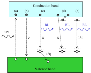
Figure 11: (Color online) Schematic picture of the main electronic processes that may be postulated for interpreting the rate equations of our decay models C2PUB v1 and v2: (a) - pump photon (UV) absorption and electron-hole pair generation; (b) - non-radiative direct electron-hole recombination; (c) radiative cross-recombination between a free electron and a trapped hole, with blue photon (BL) emission, and non-radiative thermal untrapping of holes; (d) - radiative crossed recombination between a free electron and a trapped exciton; (e) - radiative spontaneous annihilation of a trapped exciton. The constants $\gamma_{1},\gamma_{2},1/\tau_{1}$ are the dynamical rates of each process.

To interpret model C2PUBv1 we must assume instead that population 1 corresponds to excitons (i.e. e-h pairs), rather than unpaired holes, that are either self-trapped or trapped near a structural defect. In this case, population 1 can decay either by spontaneous annihilation (process e in Fig. 11) or by “crossed” recombination of a hole of the trapped pair with a mobile electron, leading to the emission of one PL photon and the simultaneous freeing of the electron of the pair (process d in Fig. 11). Both the unimolecular and the coupling terms would then be radiative with similar quantum yield, as assumed in model C2PUBv1. Although possible in principle, we believe that this C2PUBv1 model scenario is somewhat less plausible than the former (the C2PUBv2 one), both because it is more complex and because it is difficult to justify the very rapid creation of a population of trapped excitons as would be required by the initial conditions assumed in the model.

In conclusion, the main results of the investigation reported in this Article are the following: (i) we have presented strong evidence that the radiative centers involved in the blue luminescence cannot be associated with bulk oxygen vacancies or other donor impurities; (ii) we have shown, nevertheless, that a crucial role in the luminescence is played by other yet-unidentified intrinsic structural defects, such as dislocations, defect complexes, and possibly the surface; these defects likely provide the actual radiative centers; (iii) we have shown that the initial decay in the investigated excitation-intensity range is dominated by a bimolecular process, while trimolecular processes such as Auger are not significant; (iv) we have provided strong evidence that at least two separate interacting photoexcited charge populations are involved in the PL dynamics, which we interpret simply as mobile and defect-trapped charges.

References

- Savoia et al. (2009) A. Savoia, D. Paparo, P. Perna, Z. Ristic, M. Salluzzo, F. Miletto Granozio, U. Scotti di Uccio, C. Richter, S. Thiel, J. Mannhart, et al., Phys. Rev. B 80, 075110 (2009).
- Huijben et al. (2009) M. Huijben, A. Brinkman, G. Koster, G. Rijnders, H. Hilgenkamp, and D. H. A. Blank, Adv. Mater. 21, 1665 (2009).
- van Benthem et al. (2001) K. van Benthem, C. Elsässer, and R. H. French, J. Appl. Phys. 90, 6156 (2001).
- Capizzi and Frova (1970) M. Capizzi and A. Frova, Phys. Rev. Lett. 25, 1298 (1970).
- Frederikse and Hosler (1967) H. P. R. Frederikse and W. R. Hosler, Phys. Rev. 161, 822 (1967).
- Kéroack et al. (1984) D. Kéroack, Y. Lépine, and J. L. Brebner, J. Phys. C: Solid State Phys. 17, 833 (1984).
- Eagles et al. (1996) D. M. Eagles, M. Georgiev, and P. C. Petrova, Phys. Rev. B 54, 22 (1996).
- van Mechelen et al. (2008) J. L. M. van Mechelen, D. van der Marel, C. Grimaldi, A. B. Kuzmenko, N. P. Armitage, N. Reyren, H. Hagemann, and I. I. Mazin, Phys. Rev. Lett. 100, 226403 (2008).
- Ishida et al. (2008) Y. Ishida, R. Eguchi, M. Matsunami, K. Horiba, M. Taguchi, A. Chainani, Y. Senba, H. Ohashi, H. Ohta, and S. Shin, Phys. Rev. Lett. 100, 056401 (2008).
- Itoh et al. (2005) C. Itoh, M. Sasabe, H. Kida, and K. i Kan’no, J. Luminescence 112, 263 (2005).
- Stashans (2001) A. Stashans, Materials Chem. and Phys. 68, 124 (2001).
- Grabner (1969) L. Grabner, Phys. Rev. 177, 1315 (1969).
- Feng (1982) T. Feng, Phys. Rev. B 25, 627 (1982).
- Aguilar and Agullo-Lopez (1982) M. Aguilar and F. Agullo-Lopez, J. Appl. Phys. 53, 9009 (1982).
- Leonelli and Brebner (1986) R. Leonelli and J. L. Brebner, Phys. Rev. B 33, 8649 (1986).
- Hasegawa et al. (2000) T. Hasegawa, M. Shirai, and K. Tanaka, J. Luminescence 87-89, 1217 (2000).
- Deguchi et al. (2008) M. Deguchi, N. Nakajima, K. Kawakami, N. Ishimatsu, H. Maruyama, C. Moriyoshi, Y. Kuroiwa, S. Nozawa, K. Ishiji, and T. Iwazumi, Phys. Rev. B 78, 073103 (2008).
- Qiu et al. (2008) Y. Qiu, Y.-J. Jiang, G.-P. Tong, and J.-F. Zhang, Phys. Lett. A 372, 2920 (2008).
- Prócel et al. (2003) L. M. Prócel, F. Tipán, and A. Stashans, Int. J. Quantum Chemistry 91, 586 (2003).
- Eglitis et al. (2003) R. I. Eglitis, E. A. Kotomin, G. Borstel, S. E. Kapphan, and V. S. Vikhnin, Computat. Mater. Sci. 27, 81 (2003).
- Mochizuki et al. (2005) S. Mochizuki, F. Fujishiro, and S. Minami, J. Phys. Cond. Matt. 17, 923 (2005).
- Mochizuki et al. (2006) S. Mochizuki, F. Fujishiro, K. Ishiwata, and K. Shibata, Physica B 376-377, 816 (2006).
- Kan et al. (2005) D. Kan, T. Terashima, R. Kanda, A. Masuno, K. Tanaka, S. Chu, H. Kan, A. Ishizumi, Y. Kanemitsu, Y. Shimakawa, et al., Nat. Mater. 4, 816 (2005).
- Kan et al. (2006) D. Kan, R. Kanda, Y. Kanemitsu, Y. Shimakawa, M. Takano, T. Terashima, and A. Ishizumi, Appl. Phys. Lett. 88, 191916 (2006).
- Grigorjeva et al. (2004) L. Grigorjeva, D. Millers, V. Trepakov, and S. Kapphan, Ferroelectrics 304, 947 (2004).
- Zhang et al. (2008) J. Zhang, S. Walsh, C. Brookds, D. G. Schlom, and L. J. Brillson, J. Vac. Sci. Technol. B 26, 14661471 (2008).
- h. Li et al. (2007) Z. h. Li, H. t. Sun, Z. q. Xie, Y. y. Zhao, and M. Lu, Nanotechnology 18, 165703 (2007).
- Rubano et al. (2007) A. Rubano, D. Paparo, F. Miletto, U. Scotti di Uccio, and L. Marrucci, Phys. Rev. B 76, 125115 (2007).
- Rubano et al. (2008) A. Rubano, D. Paparo, M. Radović, A. Sambri, F. Miletto Granozio, U. Scotti Di Uccio, and L. Marrucci, Appl. Phys. Lett. 92, 021102 (2008).
- Yamada et al. (2009) Y. Yamada, H. Yasuda, T. Tayagaki, and Y. Kanemitsu, Phys. Rev. Lett. 102, 247401 (2009).
- Yasuda and Kanemitsu (2008) H. Yasuda and Y. Kanemitsu, Phys. Rev. B 77, 193202 (2008).
- li Zhang et al. (2009) L. li Zhang, P. Han, K. juan Jin, L. Liao, C. lian Hu, and H. bin Lu, J. Phys. D: Appl. Phys. 42, 125109 (2009).
- Blazey (1971) K. W. Blazey, Phys. Rev. Lett. 27, 146 (1971).
- Zarrabi et al. (1985) H. J. Zarrabi, W. B. Wang, and R. R. Alfano, Appl. Phys. Lett. 46, 513 (1985).
- Landsberg (1987) P. T. Landsberg, Appl. Phys. Lett. 50, 745 (1987).
- Linnros (1998) J. Linnros, J. Appl. Phys. 84, 275 (1998).
- Massé et al. (2007) N. F. Massé, A. R. Adams, and S. J. Sweeney, Appl. Phys. Lett. 90, 161113 (2007).
- Garlick (1967) G. F. J. Garlick, Rep. Prog. Phys. 30, 491 (1967).
- Hwang (2005) H. Y. Hwang, Nat. Mater. 4, 803 (2005).
- Szot et al. (2006) K. Szot, W. Speier, G. Bihlmayer, and R. Waser, Nat. Mater. 5, 312 (2006).
- Longo et al. (2008) V. M. Longo, A. T. de Figueiredo, S. de Lázaro, M. F. Gurgel, M. G. S. Costa, C. O. Paiva-Santos, J. A. Varela, E. Longo, V. R. Mastelaro, F. S. D. Vicente, et al., J. Appl. Phys. 104, 023515 (2008).
- Zhang et al. (2000) W. F. Zhang, Z. Yin, and M. S. Zhang, Appl. Phys. A 70, 93 (2000).
- Kareev et al. (2008) M. Kareev, S. Prosandeev, J. Liu, C. Gan, A. Kareev, J. W. Freeland, M. Xiao, and J. Chakhalian, Appl. Phys. Lett. 93, 061909 (2008).