The XXZ model with anti-periodic twisted boundary conditions

Abstract

We derive functional equations for the eigenvalues of the XXZ model subject to anti-diagonal twisted boundary conditions by means of fusion of transfer matrices and by Sklyanin’s method of separation of variables. Our findings coincide with those obtained using Baxter’s method and are compared to the recent solution of Galleas. As an application we study the finite size scaling of the ground-state energy of the model in the critical regime.

I Introduction

The Quantum Inverse Scattering Method (QISM) Korepin et al. (1993) provides a powerful framework for the construction of exactly solvable lattice models with the Yang-Baxter equation defining the underlying algebraic structure. This structure also serves as the basis for the solution of the spectral problem, i.e. explicit construction of eigenvalues and eigenstates, for the transfer matrices of these lattice models, by means of the algebraic Bethe ansatz. The application of this method, however, is limited to systems with a simple pseudo vacuum state which can be used as a reference state to generate the complete spectrum by application of the elements of the Yang-Baxter algebra. There exist methods to compute the spectrum of these systems which do not suffer these restrictions, e.g. Baxter’s method of commuting transfer matrices Baxter (1982) or Sklyanin’s method for separation of variables Sklyanin (1992). In these approaches, the eigenvalues are encoded into the solutions to certain functional relations which have to be solved in a second step: using the analytical properties of the transfer matrix its eigenvalues can be parametrized in terms of the roots of Bethe equations.

Recently, such alternative routes to the solution of the spectral problem of exactly solvable models have been applied to anisotropic spin chains with open ends and general non-diagonal boundary fields. Here, the boundary fields break particle number conservation and therefore the completely polarized state of spins cannot be used as a pseudo vacuum for the algebraic Bethe ansatz. Various methods have been used to determine the spectrum of the corresponding transfer matrix Nepomechie (2004); Melo et al. (2005); Murgan et al. (2006); Yang et al. (2006); Galleas (2008); Frahm et al. (2008); Baseilhac et al. (2007). Some of these methods require restrictions on the boundary fields and/or the bulk anisotropy of the spin chain to work, other approaches rely on conjectures regarding the existence of certain limits. Depending on the specific approach one obtains very different functional equations for the spectral problem and in many cases an efficient procedure for their solution is still missing.

In this paper we consider some of these approaches in a simpler setting to better understand how they are related and to assess their applicability for the solution of the spectral problem: the XXZ model with general toroidal boundary conditions is defined by the hamiltonian

$$\mathcal{H}=\sum_{j=1}^{L}\Big{[}\sigma_{j}^{x}\sigma_{j+1}^{x}+\sigma_{j}^{y}\sigma_{j+1}^{y}+\cosh\eta\,\sigma_{j}^{z}\sigma_{j+1}^{z}\Big{]}\,,\qquad\sigma^{\alpha}_{L+1}=K^{-1}\sigma^{\alpha}_{1}K$$ (1)

where $\sigma_{j}^{\alpha}$, $\alpha=x,y,z$ denote the Pauli matrices for spins $\frac{1}{2}$ at site $j$. The unitary matrix $K\in\operatorname{End}(\mathbb{C}^{2})$ determines the boundary conditions. For anti-diagonal $K$ the model is integrable but has no pseudo vacuum state (see below). It has first been solved by means of Baxter’s method Batchelor et al. (1995) and solutions to the resulting functional equations can be given in terms of the roots of Bethe ansatz equations.

The integrability of (1) is established within the QISM Korepin et al. (1993) from the Yang-Baxter algebra

$$R_{12}(\lambda-\mu)T_{1}(\lambda)T_{2}(\mu)=T_{2}(\mu)T_{1}(\lambda)R_{12}(\lambda-\mu)\,.$$ (2)

Here the monodromy matrix $T_{j}(\lambda)$ is a matrix on the auxiliary linear space $V_{j}$ with entries being the generators of the quadratic algebra. The structure constants are arranged in the $R$-matrix, $R_{jk}(\lambda)\in\operatorname{End}(V_{j}\otimes V_{k})$ which itself solves the Yang-Baxter equation

$$R_{12}(\lambda-\mu)\,R_{13}(\lambda-\nu)\,R_{23}(\mu-\nu)=R_{23}(\mu-\nu)\,R_{13}(\lambda-\nu)\,R_{12}(\lambda-\mu)\,.$$ (3)

In this paper we will use the well-known trigonometric solution for two-dimensional spaces $V_{j}$ corresponding to the six-vertex model. In this case a representation of (2) is given by local $\cal L$-matrices with $T_{a}=R_{aj}\equiv\mathcal{L}_{j}$ reading

$${\cal L}_{j}(\lambda)=\begin{pmatrix}\sinh(\lambda)S^{0}_{j}+\cosh(\lambda)S_{j}^{z}&S_{j}^{-}\\ S_{j}^{+}&\sinh(\lambda)S^{0}_{j}-\cosh(\lambda)S_{j}^{z}\end{pmatrix}\,.$$ (4)

The elements of ${\cal L}_{j}$ are operators on a two-dimensional quantum state space of a spin $\tfrac{1}{2}$, in terms of the Pauli matrices $\sigma_{j}$ they are $S^{0}_{j}=\cosh(\eta/2)I$, $S_{j}^{z}=\sinh(\eta/2)\sigma_{j}^{z}$ and $S_{j}^{\pm}=\sinh(\eta/2)\cosh(\eta/2)\sigma_{j}^{\pm}$. Using the co-multiplication of the Yang-Baxter algebra new representations can be constructed from (4): the monodromy matrix $T(\lambda)={\cal L}_{L}(\lambda)\cdots{\cal L}_{1}(\lambda)$ also satisfies (2). Note that ${\cal L}_{j}(\lambda)$ (and $T(\lambda)$) satisfies

$$\mathcal{L}_{j}(\lambda+\mathrm{i}\pi)=-\sigma^{z}_{0}\mathcal{L}_{j}(\lambda)\sigma^{z}_{0}=-\sigma^{z}_{j}\mathcal{L}_{j}(\lambda)\sigma^{z}_{j}$$ (5)

where the subscript $0$ denotes the auxiliary space.

Apart from these operator valued representations there exist $2\times 2$ c-number solutions $K$ to (2). Being independent of the spectral parameter $\lambda$ they satisfy $\big{[}R(\lambda),K\otimes K\big{]}=0$. For the six-vertex $R$-matrix, this relation has two classes of solutions, namely diagonal or anti-diagonal twist matrices $K$. Without loss of generality Alcaraz et al. (1988a); Yung and Batchelor (1995) we restrict our considerations to

$$K=\begin{pmatrix}\mathrm{e}^{-\mathrm{i}\phi}&0\\ 0&\mathrm{e}^{\mathrm{i}\phi}\end{pmatrix}\quad,\quad K=\begin{pmatrix}0&1\\ 1&0\end{pmatrix}$$ (6)

with a twist angle $\phi$ in the diagonal case.

As a consequence of (2) the transfer matrix $t(\lambda)=\operatorname{tr}_{0}[KT(\lambda)]$ generates a family of commuting operators, $[t(\lambda),t(\mu)]=0$. Therefore the spin chain hamiltonian (1) which is obtained from

$$H=2\sinh\eta\,\left.\frac{\partial\ln t(\lambda)}{\partial\lambda}\right|_{\lambda=\tfrac{\eta}{2}}-L\cosh\eta\$$ (7)

is integrable.

In the following section we will first briefly review the existing solutions of the XXZ model with anti-diagonal twisted boundary conditions followed by two different approaches to the spectral problem based on (A) the fusion hierarchy of transfer matrices Bazhanov and Reshetikhin (1989) at anisotropies $\eta=\mathrm{i}\pi/(p+1)$ with integer $p>1$ and (B) Sklyanin’s method of separation of variables Sklyanin (1992), respectively. In Section III we study the spectrum of small chains to identify the ground-state and extract the critical properties from the finite size scaling behaviour of the ground-state energy in the massless regime $\eta=\mathrm{i}\gamma$ with real $\gamma$.

II Solution of the spectral problem for anti-diagonal twist

For a diagonal twist matrix the eigenvalues and eigenstates of the transfer matrix $t(\lambda)$ can be obtained by means of the algebraic Bethe ansatz starting from the ferromagnetic so-called pseudo vacuum with polarized spins, $\langle\sigma_{j}^{z}\rangle=1$ (see e.g. Korepin et al. (1993)). For the anti-diagonal twist matrix

$$K=\begin{pmatrix}0&1\\ 1&0\end{pmatrix}\,,$$ (8)

however, the total magnetization is not a conserved quantum number. As a consequence there is no simple reference state such as the ferromagnetic one and the algebraic Bethe ansatz cannot be applied. Instead, a functional equation (called $T$$Q$-equation) for the eigenvalues $\Lambda(\lambda)$ of the transfer matrix has been obtained using Baxter’s method of commuting transfer matrices Batchelor et al. (1995); Yung and Batchelor (1995)

$$\Lambda(\lambda)q(\lambda)=\sinh^{L}\left(\lambda+\frac{\eta}{2}\right)q(\lambda-\eta)-\sinh^{L}\left(\lambda-\frac{\eta}{2}\right)q(\lambda+\eta)\,.$$ (9)

This difference equation is solved by

$$q(\lambda)=\prod_{j=1}^{L}\sinh\frac{1}{2}(\lambda-\lambda_{j})\,.$$ (10)

As a consequence of the analyticity of the transfer matrix eigenvalues it follows that the rapidities $\lambda_{j}$ are different solutions to the Bethe equations

$$\frac{\sinh^{L}(\lambda+\frac{1}{2}\eta)}{\sinh^{L}(\lambda-\frac{1}{2}\eta)}=-\prod_{k\neq j}\frac{\sinh\frac{1}{2}(\lambda-\lambda_{k}+\eta)}{\sinh\frac{1}{2}(\lambda-\lambda_{k}-\eta)}\,,\qquad\mathrm{for}\,\lambda\in\left\{\lambda_{j}\right\}_{j=1}^{L}\,.$$ (11)

(Note that these equations with an extra phase $(-1)$ and any number $M\leq L$ of rapidities $\lambda_{j}$ determine the spectrum of a staggered six-vertex model Ikhlef et al. (2008). This case, however, cannot be obtained from (1) with the twist matrices (6).) From (7) we obtain the corresponding eigenvalue of the spin chain hamiltonian (1)

$$E(\{\lambda_{j}\})=L\cosh\eta+2\sum_{j=1}^{L}\frac{\sinh\eta\,\sinh\tfrac{\eta}{2}}{\cosh{\lambda_{j}}-\cosh\tfrac{\eta}{2}}\,.$$ (12)

Recently, Galleas Galleas (2008) has proposed a different approach to solve the spectral problem of the spin chain with anti-diagonal twist. From the Yang-Baxter algebra he derives a closed set of equations for the $L-1$ zeroes $\lambda_{k}^{(1)}$ of the eigenvalues $\Lambda(\lambda)$ and a second set of $2(L-1)$ rapidities $\lambda_{\ell}^{(2)}$ defined to be the zeroes of the matrix element of a certain element of the Yang-Baxter algebra between the ferromagnetic state and the eigenstate of the model with twist

$$\left(\frac{\sinh(\lambda_{k}^{(1)}+\frac{1}{2}\eta)}{\sinh\eta}\,\frac{\sinh(\lambda_{k}^{(1)}-\frac{1}{2}\eta)}{\sinh\eta}\right)^{L-1} =-\frac{\mathrm{e}^{\frac{2\mathrm{i}\pi r}{L}}}{L}\prod_{\ell=1}^{2(L-1)}\frac{\sinh(\lambda_{\ell}^{(2)}-\lambda_{k}^{(1)})}{\sinh(\lambda_{\ell}^{(2)}-\frac{1}{2}\eta)}$$ (13)

$$\left(\frac{\sinh(\lambda_{\ell}^{(2)}+\frac{1}{2}\eta)}{\sinh\eta}\,\frac{\sinh(\lambda_{\ell}^{(2)}-\frac{1}{2}\eta)}{\sinh\eta}\right)^{L-1} =-\frac{\mathrm{e}^{\frac{2\mathrm{i}\pi r}{L}}}{L}\left(\prod_{k=1}^{L-1}\frac{\sinh(\lambda_{k}^{(1)}-\lambda_{\ell}^{(2)})}{\sinh(\lambda_{k}^{(1)}-\frac{1}{2}\eta)}\right)^{2}\,.$$

Here $r=0,\ldots,2L-1$ is a quantum number fixing the translational properties of the corresponding eigenstate. Note that as a consequence of the functional $T$$Q$-equation (9) $\lambda_{k}^{(1)}$ are the ‘hole solutions’ $\lambda=\lambda_{k}^{(1)}\notin\left\{\lambda_{j}\right\}_{j=1}^{L}$ to the Bethe equations (11).

The algebraic equations (13) involving two sets of rapidities are vaguely reminiscent of so-called nested Bethe equations for systems with higher rank symmetry. In the present case, however, the two sets of rapidities are redundant in the sense that – for an eigenstate with given $r$ – either set can be eliminated in favour of the other one. Also, unlike the string hypothesis for the Bethe rapidities $\lambda_{j}$ nothing is known about the structure of the solutions of Galleas’ equations in the thermodynamic limit $L\to\infty$, which would be a prerequisite for both numerical or analytical studies of large systems.

II.1 Fusion hierarchy and truncation identity at roots of unity

This method was first developed for the RSOS model by Bazhanov et al. Bazhanov and Reshetikhin (1989) and was adapted to spin chains by Nepomechie e.g. Nepomechie (2002, 2003). Unfortunately this method only works if the values of the crossing parameter are chosen to be roots of unity $\eta=\mathrm{i}\pi/(p+1)$. Nevertheless as in the periodic case Nepomechie (2003) the solution obtained is valid for arbitrary $\eta$ as it coincides with (9).

Because of the Yang-Baxter algebra higher spin transfer matrices of the XXZ spin chain obey a so-called fusion hierarchy, i.e. it is possible to construct a higher spin transfer matrix out of lower spin transfer matrices directly. A transfer matrix using a spin-$j$ auxiliary space is constructed using fused $\mathcal{L}$-matrices.

The fused spin-$(j,\tfrac{1}{2})$ $\mathcal{L}$-matrix for $j=\tfrac{1}{2},1,\tfrac{3}{2},\dots$ is given by Kulish and Sklyanin (1982); Kulish et al. (1981); Nepomechie (2003)

$$\mathcal{L}_{<1\cdots 2j>2j+1}(\lambda)=P^{+}_{1\cdots 2j}\mathcal{L}_{1,2j+1}(\lambda)\mathcal{L}_{2,2j+1}(\lambda+\eta)\cdots\mathcal{L}_{2j,2j+1}(\lambda+(2j-1)\eta)P^{+}_{1\cdots 2j}\quad,$$ (14)

where $P^{+}$ is the projector defined by the sum over all permutation operators for $n$ spin-$\tfrac{1}{2}$ spaces

$$P^{+}_{1\cdots n}=\frac{1}{n!}\sum_{\sigma}P_{\sigma}\quad.$$ (15)

In the same way the fusion of the twist matrix (8) is carried out yielding the spin-$j$ representation

$$K_{<1\cdots 2j>}=P^{+}_{1\cdots 2j}K_{1}K_{2}\cdots K_{2j}P^{+}_{1\cdots 2j}\quad.$$ (16)

The fused monodromy matrix for the chain then reads for $L$ lattice sites of the original hamiltonian (1)

$$T_{<1\cdots 2j>}(\lambda)=\mathcal{L}_{<1\cdots 2j>,L}(\lambda)\cdots\mathcal{L}_{<1\cdots 2j>,1}(\lambda)$$ (17)

and tracing out the auxiliary space gives the associated transfer matrix

$$t^{(j)}(\lambda)=tr_{1\cdots 2j}K_{<1\cdots 2j>}T_{<1\cdots 2j>}(\lambda)\quad.$$ (18)

For these transfer matrices the following fusion hierarchy with $j=\tfrac{1}{2},1,\tfrac{3}{2},\dots$ holds Kulish and Sklyanin (1982); Kirillov and Reshetikhin (1986, 1987); Nepomechie (2003)

$$t^{(j+1/2)}(\lambda)=t^{(j)}(\lambda)t^{(1/2)}(\lambda+2j\eta)-(d_{q}T)(\lambda+(2j-1)\eta)t^{(j-1/2)}(\lambda)\quad,$$ (19)

where $t^{(1/2)}(\lambda)\equiv t(\lambda)$ and $t^{(0)}(\lambda)\equiv I$.

On the other hand fused transfer matrices can be constructed using quantum-group theory Kulish and Reshetikhin (1983); Nepomechie (2002). The $\mathcal{L}$-matrices of higher auxiliary spins from quantum-group constructions have a simple direct relation to an $\mathcal{L}$-matrix with lower auxiliary spin at roots of unity $\eta=\mathrm{i}\pi/(p+1)$ with $p$ being an integer number. It is also possible to relate the quantum-group $\mathcal{L}$-matrices to those constructed via fusion. Resulting in the identity at roots of unity

$$B_{1\cdots p+1}A_{1\cdots p+1}\mathcal{L}_{<1\cdots p+1>,p+2}(\lambda)A^{-1}_{1\cdots p+1}B^{-1}_{1\cdots p+1}=\\ =\mu(\lambda)\begin{pmatrix}\nu(\lambda)\sigma^{z}&&\\ &B_{1\cdots p-1}A_{1\cdots p-1}\mathcal{L}_{<1\cdots p-1>,p}(\lambda+\eta)A^{-1}_{1\cdots p-1}B^{-1}_{1\cdots p-1}&\\ &&-\nu(\lambda)\sigma^{z}\\ \end{pmatrix}$$ (20)

where the entries of matrix $A$ are unnormalized Clebsch-Gordon coefficients in the decomposition of the tensor product of $2j$ spin-$1/2$ representations into a direct sum of SU(2) irreducible representations and the matrix $B$ is a diagonal matrix needed for symmetrizing Nepomechie (2002).

The function $\mu(\lambda)$ is related to the quantum determinant

$$(d_{q}T)(\lambda-\eta)=-\left(-\mu(\lambda)\right)^{L}$$ (21)

$$\mu(\lambda)\equiv-\sinh(\lambda+\tfrac{1}{2}\eta)\sinh(\lambda-\tfrac{3}{2}\eta)$$ (22)

and $\nu(\lambda)\equiv-\mu(\lambda)^{-1}(\mathrm{i}/2)^{p}\sinh\left((p+1)(\lambda-\tfrac{1}{2}\eta)\right)$ is related to the crossing parameter via $p$.

The fused twist matrices themselves obey a truncation identity similar to (20). Under the fusion procedure an anti-diagonal matrix with only 1’s as entries remains anti-diagonal with 1’s as entries after applying the transformation of the appropriate Clebsch-Gordon matrix and omitting null rows and columns, hence

$$A_{1\cdots 2j}K_{<1\cdots 2j>}A^{-1}_{1\cdots 2j}=\begin{pmatrix}&&1\\ &A_{1\cdots 2j-2}K_{<1\cdots 2j-2>}A^{-1}_{1\cdots 2j-2}&\\ 1&&\\ \end{pmatrix}\quad.$$ (23)

Identities (20) and (23) together give a truncation identity for the product of twist and monodromy matrix

$$B_{1\cdots p+1}A_{1\cdots p+1}KT_{<1\cdots p+1>,p+2}(\lambda)A^{-1}_{1\cdots p+1}B^{-1}_{1\cdots p+1}=\\ =\mu(\lambda)^{L}\begin{pmatrix}&&\left(-\nu(\lambda)\right)^{L}F\\ &B_{1\cdots p-1}A_{1\cdots p-1}KT_{<1\cdots p-1>,p}(\lambda+\eta)A^{-1}_{1\cdots p-1}B^{-1}_{1\cdots p-1}&\\ \nu(\lambda)^{L}F\\ \end{pmatrix}$$ (24)

with $F\equiv\prod_{j=1}^{L}\sigma_{j}^{z}$, and accordingly for the transfer matrix by taking the trace of (24)

$$t^{(p+1)/2}(\lambda)=-(d_{q}T)(\lambda-\eta)(-1)^{L}t^{(p-1)/2}(\lambda+\eta)\quad.$$ (25)

The fusion hierarchy (19) together with the truncation identity (25) leads to a functional relation for the transfer matrix at roots of unity for a given $p$, e.g. for $p=2$ or $j=1$ respectively this relation is

$$t(\lambda)t(\lambda+\eta)t(\lambda+2\eta)-(d_{q}T)(\lambda)t(\lambda+2\eta)+(d_{q}T)(\lambda+\eta)t(\lambda)+\\ +(-1)^{L}(d_{q}T)(\lambda-\eta)t(\lambda+\eta)=0\,.$$ (26)

Like in the RSOS model Bazhanov and Reshetikhin (1989) or the periodic XXZ chain Nepomechie (2003) the goal is to recast the general form of the functional relation (26) as a determinant of a certain matrix. This determinant being zero ensures the existence of a null eigenvector which leads to equations similar to $T$$Q$-equations.

In the case of an anti-diagonal $K$-matrix the functional relation found above cannot be recast directly, though multiplying it with itself shifted by $\mathrm{i}\pi=(p+1)\eta$ results in a recastable expression. For general $p$ this is a determinant of a $(2p+2)\times(2p+2)$ matrix reading with the eigenvalue $\Lambda$ of the transfer matrix $t$

$$\det\begin{pmatrix}\Lambda_{0}&h_{0}&0&\dots&0&-(-1)^{N}h_{1}\\ -h_{2}&\Lambda_{1}&h_{1}&&&0\\ 0&-h_{3}&\Lambda_{2}&\ddots&&\vdots\\ \vdots&&\ddots&\ddots&&0\\ 0&&&-h_{2p+1}&\Lambda_{2p}&h_{2p}\\ (-1)^{N}h_{2p+1}&0&\dots&0&-h_{0}&\Lambda_{2p+1}\\ \end{pmatrix}=0\quad.$$ (27)

In the above expression we used the shorthands

$$\Lambda_{k}\equiv \Lambda(\lambda+k\eta)$$ (28)

$$h_{k}\equiv \sinh^{L}(\lambda+k\eta-\frac{\eta}{2})\quad.$$ (29)

The definition of $h_{k}$ directly reveals $h_{k}=(-1)^{L}h_{p+1+k}$. This and the periodicity of the eigenvalue $\Lambda_{k}=-(-1)^{L}\Lambda_{p+1+k}$ following from (5) are needed to verify the equivalence of the determinant and the product of functional relations.

Let $\left(q_{0},q_{1},\ldots,q_{2p+1}\right)$ be the null eigenvector of the matrix, this yields the equations

$$\Lambda_{0}q_{0}+h_{0}q_{1}-(-1)^{L}h_{1}q_{2p+1} =0$$

$$-h_{k+1}q_{k-1}+\Lambda_{k}q_{k}+h_{k}q_{k+1} =0\quad\text{ for }k=1,\dots,2p$$ (30)

$$(-1)^{L}h_{2p+1}q_{0}-h_{0}q_{2p}+\Lambda_{2p+1}q_{2p+1} =0\quad.$$

Using the ansatz $q_{k}=q(\lambda+k\eta)$ with

$$q(\lambda)=\prod_{j=1}^{L}\sinh\frac{1}{2}(\lambda-\lambda_{j})$$ (31)

the equations (II.1) imply only a single $T$$Q$-equation

$$\Lambda(\lambda)q(\lambda)=\sinh^{L}(\lambda+\tfrac{1}{2}\eta)\,q(\lambda-\eta)-\sinh^{L}(\lambda-\tfrac{1}{2}\eta)\,q(\lambda+\eta)$$ (32)

agreeing with (9) and leading to the same Bethe ansatz equations (11). Notice the $2\pi\mathrm{i}$ periodicity of the $q$-function arising from the $2(p+1)$ rows of the matrix in (27) and the product in (31) running up to $L$ due to the structure of the upper right and lower left entries.

II.2 Separation of variables

In this section, we carry out the procedure of separation of variables, generalizing Sklyanin’s result for the XXX chain Sklyanin (1992).

We modify our definition of the monodromy matrix by introducing inhomogeneities $\delta_{j}$

$$T(\lambda)={\cal L}_{L}(\lambda-\delta_{L})\cdots{\cal L}_{1}(\lambda-\delta_{1})\ .$$ (33)

Later we will discuss the limit $\delta_{j}\to 0$. We employ the usual notation for the elements of the twisted monodromy matrix

$$\begin{pmatrix}A(\lambda)&B(\lambda)\\ C(\lambda)&D(\lambda)\end{pmatrix}=KT(\lambda)\ .$$ (34)

The Yang-Baxter algebra contains the commutation relation

$$[B(\lambda),B(\mu)]=0\ .$$ (35)

It is therefore reasonable to assume that there exists a complete set of $\lambda$-independent eigenvectors $|\ell\rangle$ of $B(\lambda)$. Note that this does not follow from the commutativity since we have not shown yet that $B(\lambda)$ is diagonalizable. By induction in $L$ we show that in the standard basis $D(\lambda)$ is lower triangular with all diagonal entries equal to zero, and $B(\lambda)$ is lower triangular with diagonal entries

$$\sinh(\lambda-x_{1}^{\ell})\cdots\sinh(\lambda-x_{L}^{\ell})\qquad\text{where}\qquad x_{j}^{\ell}=\delta_{j}\pm\tfrac{\eta}{2}\ .$$ (36)

This shows that $B(\lambda)$ is indeed diagonalizable, provided the inhomogeneities $\delta_{j}$ are mutually distinct, and that its eigenvalues are given by

$$B(\lambda)|\ell\rangle=\sinh(\lambda-x_{1}^{\ell})\cdots\sinh(\lambda-x_{L}^{\ell})|\ell\rangle\ .$$ (37)

In other words, we have defined operator-valued zeroes $\hat{x}_{j}$ of $B(\lambda)$

$$B(\lambda)=\sinh(\lambda-\hat{x}_{1})\cdots\sinh(\lambda-\hat{x}_{L})\ ,$$ (38)

where $\hat{x}_{j}=\operatorname{diag}(x_{j}^{1},\ldots,x_{j}^{2^{L}})$ in the eigenbasis of $B(\lambda)$. Since the joint spectrum of the operators $\hat{x}_{j}$ is not degenerate, any eigenvector $|\ell\rangle$ is completely determined by its eigenvalues $x_{1}^{\ell},\ldots,x_{L}^{\ell}$. We interpret the set of eigenvalues $(x_{1}^{\ell},\ldots,x_{L}^{\ell})$ of a given eigenvector $|\ell\rangle$ as a point in $\mathbb{C}^{L}$. Then the Hilbert space of the spin chain is isomorphic to the space of complex-valued functions on the set $X\subset\mathbb{C}^{L}$ of these points (for this reason the separation of variables method is also called ‘functional Bethe ansatz’). In this picture the $\hat{x}_{j}$ are the operators of multiplication by the coordinate functions $x_{j}$ in $\mathbb{C}^{L}$:

$$\hat{x}_{j}f=x_{j}f\ ,\qquad\bigl{(}\hat{x}_{j}f\bigr{)}(x^{\ell})=x_{j}^{\ell}f(x^{\ell})$$ (39)

for any function $f$ on $X$. In the following, we shall not distinguish between the operators $\hat{x}_{j}$ and the functions $x_{j}$.

We want to formulate the spectral problem for the twisted transfer matrix in the diagonal basis of the operators $x_{j}$. To this end, we first define the ‘conjugated momenta’ $X_{j}^{\pm}$ to the ‘coordinates’ $x_{j}$, which we obtain from $A(\lambda)$ and $D(\lambda)$ by substituting $\lambda=x_{j}$ ‘from the left’

$$\langle\ell|X_{j}^{-}|m\rangle=\langle\ell|A(x^{\ell}_{j})|m\rangle\qquad\text{and}\qquad\langle\ell|X_{j}^{+}|m\rangle=\langle\ell|D(x^{\ell}_{j})|m\rangle\ .$$ (40)

The following commutation relations hold, which can be shown in the same way as for the XXX case Sklyanin (1992):

$$[x_{j},x_{k}] =0\ ,$$ (41)

$$X_{j}^{\pm}x_{k} =(x_{k}\pm\eta\delta_{jk})X_{j}^{\pm}\ ,$$ (42)

$$[X_{j}^{\pm},X_{k}^{\pm}] =0\ ,$$ (43)

$$[X_{j}^{+},X_{k}^{-}] =0\quad\text{for}\quad j\neq k\ ,$$ (44)

$$X_{j}^{\pm}X_{j}^{\mp} =\Delta(x_{j}\pm\tfrac{\eta}{2})\ ,$$ (45)

where $\Delta(\lambda)$ is the quantum determinant of the twisted monodromy matrix

$$\begin{split}\Delta(\lambda)&=A(\lambda+\tfrac{\eta}{2})D(\lambda-\tfrac{\eta}{2})-B(\lambda+\tfrac{\eta}{2})C(\lambda-\tfrac{\eta}{2})\\ &=-\Bigl{[}\prod_{j=1}^{L}\sinh(\lambda-\delta_{j}+\eta)\sinh(\lambda-\delta_{j}-\eta)\Bigr{]}I\ .\end{split}$$ (46)

These commutation relations largely fix the action of the conjugated momenta $X_{j}^{\pm}$ on the eigenvectors of the operators $x_{j}$. The remaining freedom is due to the fact that the $x_{j}$-eigenvectors are determined only up to phase factors (Sklyanin, 1992, Thm. 3.4). (In the functional language changing these phase factors corresponds to multiplying all functions with an arbitrary function which has no zeroes.) We will now reconstruct the conjugated momenta from the commutation relations. This will allow us to formulate the spectral problem for the twisted transfer matrix in the $x_{j}$-eigenbasis without knowing the change of bases explicitly. Let $\omega$ be the function $\omega\equiv 1$ on $X$, and define the functions $\Delta_{j}^{\pm}$ by

$$\Delta_{j}^{\pm}(x)=\bigl{(}X_{j}^{\pm}\omega\bigr{)}(x)\ .$$ (47)

Equation (42) implies

$$\bigl{(}X_{j}^{\pm}f\bigr{)}(x)=\Delta_{j}^{\pm}(x)f(E_{j}^{\pm}x)$$ (48)

for any function $f$ on $X$. Here we have introduced the shift operators $E_{j}^{\pm}$

$$E_{j}^{\pm}\colon(x_{1},\ldots,x_{j},\ldots,x_{L})\longmapsto(x_{1},\ldots,x_{j}\pm\eta,\ldots,x_{L})\ .$$ (49)

As the functions $f$ are defined only on $X$,

$$\Delta_{j}^{\pm}(x)=0\qquad\text{whenever}\qquad E_{j}^{\pm}x\notin X$$ (50)

must hold. The commutation relations (43)–(45) translate into the following conditions on the functions $\Delta_{j}^{\pm}$:

$$\Delta_{j}^{\pm}(x)\Delta_{k}^{\pm}(E_{j}^{\pm}x) =\Delta_{k}^{\pm}(x)\Delta_{j}^{\pm}(E_{k}^{\pm}x)\ ,$$ (51)

$$\Delta_{j}^{+}(x)\Delta_{k}^{-}(E_{j}^{+}x) =\Delta_{k}^{-}(x)\Delta_{j}^{+}(E_{k}^{-}x)\quad\text{for}\quad j\neq k\ ,$$ (52)

$$\Delta_{j}^{\pm}(x)\Delta_{j}^{\mp}(E_{j}^{\pm}x) =\Delta(x_{j}\pm\tfrac{\eta}{2})\ .$$ (53)

We make the following ansatz: Let the functions $\Delta_{j}^{\pm}$ be defined as

$$\Delta_{j}^{\pm}(x)=\Delta_{\pm}(x_{j})\ ,$$ (54)

where

$$\Delta_{\pm}(\lambda)=\xi_{\pm}\sinh(\lambda-\delta_{1}\mp\tfrac{\eta}{2})\cdots\sinh(\lambda-\delta_{L}\mp\tfrac{\eta}{2})\ .$$ (55)

In this definition, the constants $\xi_{\pm}$ are an arbitrary factorization of the determinant of the twist matrix

$$\xi_{+}\xi_{-}=\det(K)=-1\ ,$$ (56)

and the functions $\Delta_{\pm}$ factorize the quantum determinant of the monodromy matrix in the following sense:

$$\Delta_{+}(\delta_{j}-\tfrac{\eta}{2})\Delta_{-}(\delta_{j}+\tfrac{\eta}{2})=\Delta(\delta_{j})\ .$$ (57)

This ansatz satisfies the conditions given in Eqs. (50)–(53).

We now return to the spectral problem for the twisted transfer matrix

$$t(\lambda)q(x)=\Lambda(\lambda)q(x)\ .$$ (58)

The eigenvector $q$ is in our representation a complex-valued function on $X$. We substitute $\lambda=x_{j}$ from the left and obtain

$$\Lambda(x_{j})q(x)=\Delta_{+}(x_{j})q(E_{j}^{+}x)+\Delta_{-}(x_{j})q(E_{j}^{-}x)\ .$$ (59)

The coefficients $\Delta_{\pm}$ now depend on only one coordinate $x_{j}$. This is due to the particular solution $\Delta_{j}^{\pm}$ to the conditions (50)–(53) chosen in Eqs. (54)–(56), for a generic solution it would not have been the case. The last equation (59) suggests the separation of variables ansatz

$$q(x)=q_{L}(x_{L})\cdots q_{1}(x_{1})\ .$$ (60)

It remains to solve a set of one-dimensional problems

$$\Lambda(x_{j})q_{j}(x_{j})=\Delta_{+}(x_{j})q_{j}(x_{j}+\eta)+\Delta_{-}(x_{j})q_{j}(x_{j}-\eta)\ ,\qquad j=1,\ldots,L\ ,$$ (61)

which we recognize as the $T$$Q$-equation (9), evaluated on the discrete lattice $X$.

Recalling that $x_{j}$ takes the values $\delta_{j}\pm\eta/2$ and using $\Delta_{\pm}(\delta_{j}\pm\eta/2)=0$, we see that the finite-difference equation (61) takes the form of a homogeneous system of linear equations

$$\begin{pmatrix}\Lambda(\delta_{j}+\tfrac{\eta}{2})&-\Delta_{-}(\delta_{j}+\tfrac{\eta}{2})\\ -\Delta_{+}(\delta_{j}-\tfrac{\eta}{2})&\Lambda(\delta_{j}-\tfrac{\eta}{2})\end{pmatrix}\begin{pmatrix}q_{j}(\delta_{j}+\tfrac{\eta}{2})\\ q_{j}(\delta_{j}-\tfrac{\eta}{2})\end{pmatrix}=0\ .$$ (62)

For a nontrivial solution its determinant has to vanish

$$\Lambda(\delta_{j}+\tfrac{\eta}{2})\Lambda(\delta_{j}-\tfrac{\eta}{2})=\Delta(\delta_{j})\ ,\qquad j=1,\ldots,L$$ (63)

(we have used equation (57)). The eigenvalue $\Lambda(\lambda)$ is of the form

$$\Lambda(\lambda)=\Lambda_{-L+1}\mathrm{e}^{(-L+1)\lambda}+\Lambda_{-L+3}\mathrm{e}^{(-L+3)\lambda}+\cdots+\Lambda_{L-1}\mathrm{e}^{(L-1)\lambda}\ .$$ (64)

The $L$ coefficients $\Lambda_{j}$ have to be determined from the $L$ equations (63). Each of these equations defines a quadratic form in the $L$-dimensional complex space of the coefficients of $\Lambda(\lambda)$ (see also Frahm et al. (2008)). These quadratic forms intersect at $2^{L}$ points, which correspond to the $2^{L}$ eigenvalues $\Lambda(\lambda)$. (Note that the eigenvalues of the transfer matrix are non-degenerate for the anti-diagonal twist. This explains why the method of separation of variables does not suffer the so-called ‘completeness problem’ of the algebraic Bethe ansatz. In the case of diagonal twist matrices the method cannot be applied since the operator $B(\lambda)$ has only $L-1$ zeroes.)

Finally, we want to remove the inhomogeneities $\delta_{j}$, which were not present in the original problem related to the spin chain (1). Simply putting them all to zero is not possible since then the equations (63) are no longer independent. Instead, we consider the equation

$$\Lambda(\delta+\tfrac{\eta}{2})\Lambda(\delta-\tfrac{\eta}{2})=-\sinh^{L}(\delta-\eta)\sinh^{L}(\delta+\eta)$$ (65)

and its derivatives w.r.t. $\delta$ up to order $L-1$, evaluated at $\delta=0$. For small systems we have verified that this procedure does give the correct eigenvalues $\Lambda(\lambda)$.

III Finite-size scaling of the ground-state energy

III.1 Solution of the Bethe equations

As an application of the solution of the spectral problem we now study the description of the ground-state in terms of the solutions to the Bethe equations. We start by solving these equations (11) for the complex Bethe rapidities $\{\lambda_{j}\}_{j=1}^{L}$ numerically for small systems.

In the antiferromagnetic massive regime, described by real $\eta$, the Bethe rapidities of the ground-states, and only those, are purely imaginary for small system sizes and small values of $\eta$. As the system size grows or for larger values of $\eta$ two of the rapidities in the ground-state form a single ‘2-string’ of rapidities symmetric to the imaginary axis, $\lambda\pm\eta/2$. Computing the energy of this state one obtains a system size independent contribution. This is the energy of a domain wall, corresponding to the interfacial tension in the six-vertex model computed in Ref. Batchelor et al., 1995.

Here we concentrate on the massless case, i.e. $\eta=\mathrm{i}\gamma$ with real $\gamma$. In Figures 1 and 2 some results for up to 4 lattice sites and $\eta=\mathrm{i}\pi/4$ are shown. As a consequence of the periodicity of the Bethe equations the set $\{\lambda_{j}+\mathrm{i}\pi\}_{j=1}^{L}$ is also a solution which parametrizes a second state corresponding to a different eigenvalue (9) of the transfer matrix but has the same energy (12). As the lattice size increases, we find that all Bethe rapidities of the two ground-states have imaginary parts $0$ or $\pi$. Below we will use this observation to study the finite size scaling behaviour of the ground-state energy. For excited states we have not identified such a pattern which would be necessary for a systematic analysis of the excitation spectrum starting from the Bethe equations (11).

Also shown in Figures 1 and 2 are the corresponding solutions to Galleas’ equations (13), i.e. the two sets of rapidities $\{\lambda_{j}^{(1)}\}_{j=1}^{L-1}$, $\{\lambda_{j}^{(2)}\}_{j=1}^{2(L-1)}$ and the quantum number $r$. Galleas’ equations are invariant under separate shifts of the two sets by $\mathrm{i}\pi$, therefore each rapidity appears twice and $\lambda$ and $\lambda+\mathrm{i}\pi$ have to be identified. In this parametrization, the pairs of degenerate solutions are given by the same rapidities $\lambda_{j}^{(1)}$ and $\lambda_{j}^{(2)}$, but their values of $r$ differ by $L$. Again, the distribution of the roots of (13) in the complex plane does not appear to follow a simple scheme as the system size increases, not even for the the ground-state. Therefore, this approach is of limited use only to study the spectrum of long chains.

Figure 1: Distribution of the Bethe rapidities $\lambda_{j}$ ($\bullet$) and the rapidities ${\lambda^{(1)}}_{j}$ ($\square$) and ${\lambda^{(2)}}_{j}$ ($\triangledown$) in the massless regime with $\eta=\mathrm{i}\pi/4$ for two lattice sites.

(a) $L=3$, $\eta=\mathrm{i}\pi/4$                                (b) $L=4$, $\eta=\mathrm{i}\pi/4$

Figure 2: Distribution of the Bethe rapidities $\lambda_{j}$ ($\bullet$) and the rapidities ${\lambda^{(1)}}_{j}$ ($\square$) and ${\lambda^{(2)}}_{j}$ ($\triangledown$) for the ground-state in the massless regime with $\eta=\mathrm{i}\pi/4$ for (a) three lattice sites and (b) four lattice sites.

To proceed, we parametrize Bethe roots corresponding to the ground-states as follows: let $\mu_{j}$, $j=1,\ldots,m$ be the real Bethe rapidities and $\nu_{j}$, $j=1,\ldots,n$ the real parts of the Bethe rapidities with imaginary part $\pi$. For even system sizes $L$ we have $m=n=L/2$, for odd system sizes we have $m=(L\mp 1)/2$, $n=(L\pm 1)/2$ for two ground-state configurations. We take the logarithm of the Bethe equations (11) and obtain

$$L\Phi(\mu_{j}) =2\pi I_{j}+\sum_{k=1}^{m}\Theta(\mu_{j}-\mu_{k})+\sum_{k=1}^{n}\widetilde{\Theta}(\mu_{j}-\nu_{k})\ ,\qquad j=1,\dots,m\ ,$$ (66)

$$L\Phi(\nu_{k}) =2\pi J_{k}+\sum_{\ell=1}^{m}\widetilde{\Theta}(\nu_{k}-\mu_{\ell})+\sum_{\ell=1}^{n}\Theta(\nu_{k}-\nu_{\ell})\ ,\qquad k=1,\dots,n\ ,$$

where

$$\Phi(\lambda) =-\mathrm{i}\ln\Bigl{[}\frac{\sinh(\lambda-\tfrac{\mathrm{i}\gamma}{2})}{\sinh(\lambda+\tfrac{\mathrm{i}\gamma}{2})}\Bigr{]}=\pi+2\arctan[\tanh(\lambda)\cot(\tfrac{\gamma}{2})]\ ,$$

$$\Theta(\lambda) =-\mathrm{i}\ln\Bigl{[}\frac{\sinh[\tfrac{1}{2}(\lambda-\mathrm{i}\gamma)]}{\sinh[\tfrac{1}{2}(\lambda+\mathrm{i}\gamma)]}\Bigr{]}=\pi+2\arctan[\tanh(\tfrac{\lambda}{2})\cot(\tfrac{\gamma}{2})]\ ,$$

$$\widetilde{\Theta}(\lambda) =-\mathrm{i}\ln\Bigl{[}\frac{\sinh[\tfrac{1}{2}(\lambda+\mathrm{i}\pi-\mathrm{i}\gamma)]}{\sinh[\tfrac{1}{2}(\lambda+\mathrm{i}\pi+\mathrm{i}\gamma)]}\Bigr{]}=2\arctan[\tanh(\tfrac{\lambda}{2})\cot(\tfrac{\gamma}{2}+\tfrac{\pi}{2})]\ .$$

We have chosen the branch of the logarithm in such a way that the functions $\Phi$, $\Theta$ and $\widetilde{\Theta}$ are monotonically increasing. Here $\arctan$ denotes the principal branch of the inverse tangent taking values between $-\pi/2$ and $\pi/2$. Our numerical solutions for small chains show that the Bethe integers $I_{j}$ and $J_{k}$ in (66) follow a simple pattern: for even system sizes, one ground-state is obtained with

$$I_{j} =j-1 \text{ for }j=1,\dots,\frac{L}{2}$$ (67)

$$J_{k} =k \text{ for }k=1,\dots,\frac{L}{2}$$

while for odd $L$

$$I_{j} =j-1 \text{ for }j=1,\dots,\frac{L+1}{2}$$ (68)

$$J_{k} =k \text{ for }k=1,\dots,\frac{L-1}{2}$$

The second ground-state is obtained by interchanging the sets $\{I_{j}\}$ and $\{J_{k}\}$.

In the thermodynamic limit we can solve the logarithmic Bethe equations (66) analytically. Rewriting them as

$$Y(\mu_{j})=I_{j}\ ,\qquad Z(\nu_{j})=J_{j}\$$ (69)

with the ‘counting functions’ $Y$ and $Z$ which satisfy $Y(-\infty)=Z(-\infty)=0$ and $Y(+\infty)=m$, $Z(+\infty)=n$. Assuming that the distributions of the rapidities $\mu_{j}$ and $\nu_{j}$ can be described by countinuous densities $\rho$ and $\sigma$ in the thermodynamic limit they are given by the derivatives of the counting functions

$$\rho(\lambda)=\frac{1}{L}Y^{\prime}(\lambda)\ ,\qquad\sigma(\lambda)=\frac{1}{L}Z^{\prime}(\lambda)\ .$$ (70)

The logarithmic Bethe equations become a pair of coupled integral equations

$$2\pi\rho(\lambda) =\Phi^{\prime}(\lambda)-\int\mathrm{d}\lambda^{\prime}\,\Theta^{\prime}(\lambda-\lambda^{\prime})\rho(\lambda^{\prime})-\int\mathrm{d}\lambda^{\prime}\,\widetilde{\Theta}^{\prime}(\lambda-\lambda^{\prime})\sigma(\lambda^{\prime})\ ,$$ (71)

$$2\pi\sigma(\lambda) =\Phi^{\prime}(\lambda)-\int\mathrm{d}\lambda^{\prime}\,\widetilde{\Theta}^{\prime}(\lambda-\lambda^{\prime})\rho(\lambda^{\prime})-\int\mathrm{d}\lambda^{\prime}\,\Theta^{\prime}(\lambda-\lambda^{\prime})\sigma(\lambda^{\prime})\$$

which can be solved by Fourier transform, yielding

$$\rho(\lambda)=\sigma(\lambda)=\frac{1}{2\gamma}\frac{1}{\cosh(\lambda\pi/\gamma)}\ .$$ (72)

Here we have assumed without loss of generality $0<\gamma<\pi$. For the ground-state energy per lattice site in the thermodynamic limit we find with (12)

$$\varepsilon_{\infty}=\cos\gamma-\frac{\sin\gamma}{\gamma}\int\frac{\mathrm{d}\lambda}{\cosh(\lambda\pi/\gamma)}\,\frac{2\sin\gamma}{\cosh(2\lambda)-\cos\gamma}\ .$$ (73)

This agrees with the result for the untwisted chain Yang and Yang (1966), though the distribution of the Bethe rapidities is different.

III.2 Conformal field theory

The low energy effective field theory for the XXZ model in the massless regime, $-1<\cos\gamma\leq 1$, is well known to be that of a free boson with compactification radius $\sqrt{2\pi}R=\sqrt{(\pi-\gamma)/\pi}$. Conformal field theory predicts the finite size scaling of the energies of the ground-state and the low lying excitations Affleck (1986); Blöte et al. (1986) for a system with periodic boundary conditions as

$$E_{h\bar{h}}(L)=L\,e_{\infty}-\frac{\pi v_{F}}{6L}\,c+\frac{2\pi v_{F}}{L}\,(h+\bar{h})+o(L^{-1})$$ (74)

where $e_{\infty}$ is the energy density in the ground-state, which is in our case given by Eq. (73), and $v_{F}=\frac{2\pi}{\gamma}\,\sin\gamma$ is the ‘Fermi’ velocity of elementary excitations in the system. The universal number $c$ is the central charge of the conformal field theory, for the free boson it is $c=1$.

From the energies appearing in the spectrum (74) for a given lattice realization of the field theory one can identify the operator content of the latter: $h$ and $\bar{h}$ are the conformal weights of primary operators of the CFT. By choosing particular boundary conditions one obtains different sectors of the theory (i.e. certain representations of the global symmetry group $O(2)$ of the model (1)). For diagonal boundary conditions (6) with $\phi=0$ and $\pi/2$ the symmetry of the bulk Hamiltonian (1) is preserved and the spectrum is given in terms of the highest weights of two commuting $U(1)$ Kac-Moody algebras. The scaling dimensions of the primary operators ${\cal O}_{n,m}$ are given in terms of the eigenvalues $n$ of the $U(1)$ charge operator $\frac{1}{2}\sum_{j}\sigma_{j}^{z}$ and momentum $2\pi m/L$ by

$$x_{n,m}=h_{n,m}+\bar{h}_{n,m}=\pi R^{2}n^{2}+\frac{m^{2}}{4\pi R^{2}}$$ (75)

($m$ takes integer (half odd integer) values for $\phi=0$ ($\phi=\pi/2$)). A diagonal twist (6) with angle $\phi\neq 0,\pi/2$ breaks the global symmetry to $SO(2)$. The dimensions of primary operators are $x_{n,m+\phi/\pi}$. As a consequence the finite size scaling of the lowest energy state energy is changed to $E_{\mathrm{GS}}(L)=L\,e_{\infty}-{\pi v_{F}}\,c_{\mathrm{eff}}/{6L}$ with an effective central charge Alcaraz et al. (1988b)

$$c_{\mathrm{eff}}=1-12\,x_{0,\phi/\pi}=1-\frac{6\phi^{2}}{\pi(\pi-\gamma)}\,,\quad|\phi|\leq\frac{\pi}{2}.$$ (76)

In the case of anti-diagonal twisted boundary conditions the $O(2)$ bulk symmetry is broken to $Z_{2}\otimes Z_{2}$ with the factors being generated by rotation around the $z$-axis by $\pi$ and a global spin flip, respectively. The low-energy spectrum is that of a $U(1)$-twisted Kac-Moody algebra without conserved charge. In this case the conformal weights are Alcaraz et al. (1988a)

$$(h,\bar{h})_{k_{1},k_{2}}=\left(\frac{(4k_{1}+1)^{2}}{16},\frac{(4k_{2}+1)^{2}}{16}\right)$$ (77)

with integer $k_{i}$.

We have solved the Bethe equations (66) for the ground-state of the spin chain numerically for system sizes up to $L=500$. From (77) we expect the lowest energy state to be that with conformal weights $(h,\bar{h})_{0,0}=(\frac{1}{16},\frac{1}{16})$ for both even and odd number of lattice sites. With (74) this leads to the CFT prediction for the finite size scaling of the energy

$$E_{\mathrm{GS}}(L)=L\epsilon_{\infty}+\frac{\pi v_{F}}{6L}\left(-\frac{1}{2}+12\left(\frac{1}{16}+\frac{1}{16}\right)+R(L)\right)\,,\qquad\lim_{L\to\infty}R(L)=0.$$ (78)

The resulting effective central charge $c_{\mathrm{eff}}=-1/2$ is independent of the anisotropy which agrees nicely with our numerical data presented in Table 1. In the isotropic limit of the XXZ model, $\gamma\to 0$, the spectrum depends only on the eigenvalues of the twist matrix (8) and therefore the anti-diagonal twist is unitary equivalent to a diagonal one with twist-angle $\pi$ (76).

The corrections $R(L)$ to the scaling (78) are a consequence of the fact that the lattice hamiltonian (1) differs from the conformally invariant hamiltonian of the continuum theory by terms involving irrelevant operators Cardy (1986). Perturbation of the conformal theory with an irrelevant operator with scaling dimension $x>2$ leads to $R(L)\propto L^{2-x}$. Therefore, by analyzing these corrections in the numerical data one can identify the leading irrelevant perturbation of the lattice hamiltonian.

For the periodic XXZ chain and the model with diagonal twist the corrections to scaling vanish with an exponent $x-2=\max(4\gamma/(\pi-\gamma),2)$ Woynarovich and Eckle (1987); Alcaraz et al. (1988b). The hamiltonian of the XXZ model with anti-periodic twisted boundary conditions, however, is related to the thermal operator of the Ashkin-Teller model and the leading corrections to scaling $R(L)$ are generated by the operator ${\cal O}_{0,2}$ Alcaraz et al. (1987), i.e.

$$R(L)\propto L^{2-x_{0,2}}=L^{-\frac{2\gamma}{\pi-\gamma}}\,.$$ (79)

As shown in Figure 3, this provides an excellent fit for our numerical data. The dependence (79) on the anisotropy parameter explains the slow convergence towards $c_{\mathrm{eff}}$ in Table 1 as $\gamma\to 0$.

Table 1: Finite size scaling of the ground-state energy in systems with even (odd) number of sites for several values of the anisotropy $\gamma$: Shown are the numerical results for $-c_{\mathrm{eff}}=(6/\pi v_{F})\,L(E_{0}(L)-L\,e_{\infty})$ for lattices of size $L$ together with the extrapolation to $L=\infty$.

L	$\gamma=\pi/8$	$\gamma=\pi/4$	$\gamma=3\pi/8$	$\gamma=\pi/2$
30	0.59536849	0.53046883	0.50367226	0.50009141
60	0.57644644	0.51909229	0.50156060	0.50002285
120	0.56176871	0.51200578	0.50067152	0.50000571
240	0.55014811	0.50755893	0.50029553	0.50000143
480	0.54084022	0.50476118	0.50014993	0.50000035
extr.	0.51(2)	0.500(1)	0.5000(1)	0.500000(1)
29	0.40781510	0.46933409	0.49658570	0.50009782
59	0.42572231	0.48079424	0.49850626	0.50002363
119	0.43973453	0.48794414	0.49934855	0.50000494
239	0.45088912	0.49242107	0.49972106	0.50000144
479	0.45987007	0.49523121	0.49990010	0.50000036
extr.	0.48(2)	0.499(1)	0.4999(1)	0.500000(1)

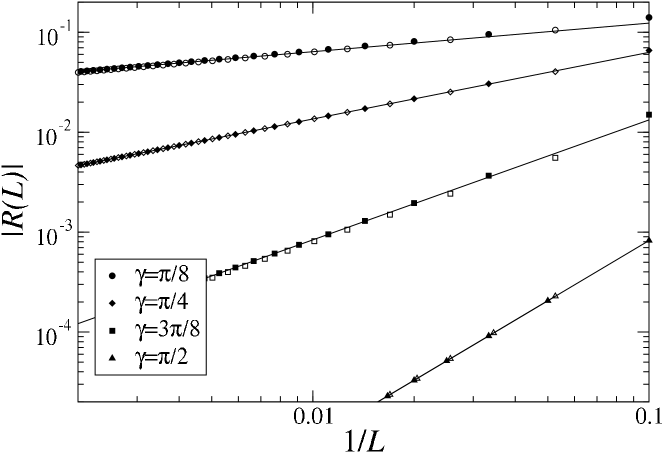
Figure 3: Corrections to the scaling of the ground-state energy: Closed (open) symbols are numerical finite size data for even (odd) system sizes, lines are fits to a power law $R(L)\propto L^{-2\gamma/(\pi-\gamma)}$.

IV Summary and Conclusion

For the XXZ spin chain with anti-diagonal twist which does not allow for a solution of the spectral problem by means of the algebraic Bethe ansatz due to the lack of a reference state we have derived the functional equations (9), originally obtained using Baxter’s method of commuting transfer matrices, employing different methods: restricting the anisotropy to roots of unity $\eta=\mathrm{i}\pi/(p+1)$ the $T$$Q$-equation of Batchelor et al. (1995) was obtained by truncation of the fusion hierarchy. In a second approach, namely through Sklyanin’s separation of variables, we have used a representation of the Yang-Baxter algebra on a space of symmetric functions defined on a discrete lattice. In this formulation the spectral problem could again be recast in the form of the same $T$$Q$-equation (61) – in this case, however, it has to be solved on the lattice of singular points of this functional equation only. This is unlike the situation for the spin chain with open boundaries and non-diagonal boundary fields where different functional equations have been found within different approaches.

In the lattice formulation of the $T$$Q$-equation arising from the separation of variables the computation of the eigenvalues amounts to finding roots of $L$ coupled polynomial equations (63), therefore this approach appears to be best suited to determine the spectrum of small systems. A similar limitation holds for the recent approach of Galleas Galleas (2008). For an efficient solution of the $T$$Q$-equation in the thermodynamic limit the parametrization (10) or (31) of the solution to the functional equations has to be used which leads to $L$ algebraic Bethe equations (11). At least for the ground-state energy of the spin chain these equations can be solved, e.g. to obtain the interfacial tension of the six-vertex model (see Batchelor et al. (1995)) or to identify the operator content of the low energy effective theory in the massless regime.

Note, that together with the eigenvalues $\Lambda(\lambda)$ one obtains the functions $q(\lambda)$ from the $T$$Q$-equation in either approach. It is quite clear from the separation of variables that these functions contain the complete information on the eigenstates of the transfer matrix. However, unlike the situation with the algebraic Bethe ansatz, where one has an expression for the eigenstates in terms of the generators of the Yang-Baxter algebra, the explicit transformation from the $q$-functions to state vectors in the Hilbert space of the spin chain is not known.