Henry’s law, surface tension, and surface adsorption in dilute binary mixtures

Abstract

Equilibrium properties of dilute binary fluid mixtures are studied in two-phase states on the basis of a Helmholtz free energy including the gradient free energy. The solute partitioning between gas and liquid (Henry’s law) and the surface tension change $\Delta\gamma$ are discussed. A derivation of the Gibbs law $\Delta\gamma=-T\Gamma$ is given with $\Gamma$ being the surface adsorption. Calculated quantities include the derivatives $dT_{c}/dX$ and $dp_{c}/dX$ of the critical temperature and pressure with respect to the solute molar fraction $X$ and the temperature-derivative $(\partial\gamma/\partial T)_{{\rm cx},p}$ of the surface tension at fixed pressure $p$ on the coexistence surface. Here $(\partial\gamma/\partial T)_{{\rm cx},p}$ can be both positive and negative, depending on the solute molecular size and the solute-solvent interaction, and diverges on the azeptropic line. Near the solvent critical point, it is proportional to $(dp_{c}/dX)/K_{\rm Kr}$, where $K_{\rm Kr}$ is the Krichevskii parameter. Explicit expressions are given for all these quantities in the van der Waals model.

I Introduction

Many problems in physics and engineering involve dilute solutions. In one-phase states, the critical behavior of dilute fluid mixtures have been studied extensively Griffiths ; Anisimov ; Onukibook , where crossover occurs from pure-fluid behavior to binary-mixture behavior on approaching the critical line. In two-phase states, it has been of great interest how a solute is partitioned between gas and liquid and how it is adsorbed in or repelled from the interface region Sengers1 ; SengersReview ; De ; Harvey .

In the dilute limit, the solute-solute interaction may be neglected for nonelectrolytes. Nevertheless, the two-phase behavior is still highly nontrivial, depending sensitively on the detail of the solute-solvent interaction. In particular, the surface tension change $\Delta\gamma$ due to a solute is related to the excess solute adsorption Gibbs . To understand such effects, we will present a simple Ginzburg-Landau theory of dilute mixtures including the gradient free energy Onukibook . As is well-known vander , van der Waals originally constructed such a theory for pure fluids to describe a gas-liquid interface and to calculate the surface tension $\gamma$. For binary mixtures it is moreover possible to calculate the solute density profile around an interface, which should satisfy the Gibbs adsorption law. In this approach solute partitioning between the two phases may be examined systematically.

In fluid hydrodynamics involving a gas-liquid interface, it is crucial how the surface tension varies on the surface as a function of ambient temperature, concentration, and pressure, since its variation induces a Marangoni flow Levich ; Straub . However, the present author is not aware of any fundamental theory on the surface variation of $\gamma$ in fluid mixtures in nonequilibrium. Hence we will also calculate the surface-tension derivative $(\partial\gamma/\partial T)_{{\rm cx},p}$ with respect to the temperature $T$ at fixed pressure $p$ in two-phase coexistence Maran .

In Section II, we will present a Ginzburg-Landau model to calculate how the coexistence surface and the critical line are formed with addition of the second component. Mean-field critical behavior of dilute mixtures will be discussed, where the so-called Krichevskii parameter Sengers1 ; SengersReview ; De ; Harvey ; Kri ; OC ; Shock will be of crucial relevance. On the basis of the Gibbs adsorption law to be derived in Appendix A, general expressions for the surface tension variations on the coexistence surface will be given. In Section III, use will be made of the van der Waals free energy of dilute mixtures Sengers ; De supplemented with the gradient free energy. It will give explicit expressions for all the physical quantities discussed in Section II, in terms of two dimensionless parameters characterizing the solute-solvent interaction. In Appendix B, correlation-function expressions for thermodynamic derivatives including that of the Krichevskii parameter will be given Onukibook ; OnukiJLTP .

II Theoretical background

II.1 Ginzburg-Landau theory

This paper treats dilute nonelectrolyte binary mixtures with short-range interactions undergoing the gas-liquid transition. The number densities of the two components are written as $n_{1}$ and $n_{2}$ with $n_{2}\ll n_{1}$, which are coarse-grained variables changing smoothly in space. A Ginzburg-Landau free theory is used to describe two-phase coexistence. A number of authors calculated the surface tension of mixtures by combining an equation of state and the gradient theory Carley ; Sahimi ; Strenby .

Hereafter the Boltzmann constant will be set equal to unity. The free energy functional $F=F\{n_{1},n_{2}\}$ depends on $n_{1}$ and $n_{2}$ as

$$F=\int d{\mbox{\boldmath$r$}}\bigg{[}f+\frac{T}{2}\sum_{i,j=1,2}D_{ij}\nabla n_{i}\cdot\nabla n_{j}\bigg{]}.$$ (2.1)

The first term $f=f(n_{1},n_{2},T)$ in the brackets is the Helmholtz free energy density dependent on the densities and the temperature $T$. The gradient terms are needed to account for a free-energy increase due to density inhomogeneity. The coefficients $D_{11}$, $D_{12}=D_{21}$, and $D_{22}$ are assumed to be constants independent of the densities. In the dilute case $n_{2}\ll n_{1}$, the following form is assumed:

$$f=f_{0}(n_{1},T)+Tn_{2}[\ln(n_{2}\lambda_{2}^{3})-1+\varphi(n_{1},T)].$$ (2.2)

Here the van der Waals attractive interactions among the molecules of the species 2 $(\propto n_{2}^{2}$) are neglected. The $f_{0}(n_{1},T)$ is the Helmholtz free energy density of the one-component (pure) fluid of the species 1 and $\lambda_{2}=\hbar(2\pi/m_{2}T)^{1/2}$ ($\hbar$ being the Planck constant) is the de Broglie length of the species 2. The term $Tn_{2}\varphi$ arises from the solute-solvent interaction, where $\varphi=\varphi(n_{1},T)$ is independent of $n_{2}$ (see the next section for its van der Waals expression).

For the free energy density $f$ in Eq.(2.2) the chemical potentials of the two components (without the gradient contributions) are expressed as

$$\mu_{1} = \frac{\partial f}{\partial n_{1}}=\mu_{0}(n_{1},T)+Tn_{2}\varphi^{\prime}(n_{1},T),$$ (2.3)

$${\mu}_{2} = \frac{\partial f}{\partial n_{2}}=T\ln(n_{2}\lambda_{2}^{3})+T\varphi(n_{1},T),$$ (2.4)

where $\mu_{0}=\partial f_{0}/\partial n_{1}$ is the chemical potential of the pure fluid and $\varphi^{\prime}=\partial\varphi/\partial n_{1}$ in $\mu_{1}$. Note that $\mu_{2}$ tends to $-\infty$ logarithmically in the low density limit $n_{2}\rightarrow 0$. The pressure $p=n_{1}\mu_{1}+n_{2}\mu_{2}-f$ is expressed as

$$p=n_{1}\mu_{0}-f_{0}+Tn_{2}(1+n_{1}\varphi^{\prime}),$$ (2.5)

where the last term is the solute correction. For the free energy functional $F$ in Eq.(2.1) the generalized chemical potentials including the gradient contributions read

$$\hat{\mu}_{i}=\frac{\delta F}{\delta n_{i}}=\mu_{i}-T\sum_{j=1,2}D_{ij}\nabla^{2}n_{j}\quad(i=1,2),$$ (2.6)

which are homogeneous in space in equilibrium. The usual chemical potentials $\mu_{1}$ and $\mu_{2}$ deviate from $\hat{\mu}_{1}$ and $\hat{\mu}_{2}$ in the interface region. Originally, van der Waals set up the following interface equation for pure fluids vander ,

$$\mu_{0}(n,T)-TD_{11}n^{\prime\prime}=\mu_{\rm cx}^{0}(T),$$ (2.7)

where $\mu_{\rm cx}^{0}$ is the chemical potential on the coexistence curve $p=p_{\rm cx}^{0}(T)$ of the pure fluid. The density $n(z)$ changes along the $z$ axis and $n^{\prime\prime}=d^{2}n/dz^{2}$. Our equations in Eq.(2.6) lead to the van der Waals interface equation (2.7) for $n_{1}=n(z)$ and $n_{2}=0$.

In this paper a small parameter $\zeta$ is defined as

$$\zeta=\lambda_{2}^{-3}e^{\hat{\mu}_{2}/T},$$ (2.8)

which has the dimension of density. The solute density $n_{2}$ is expressed as as

$$n_{2} = \zeta\exp\bigg{[}-\varphi(n_{1},T)+{D_{12}}\nabla^{2}n_{1}+{D_{22}}\nabla^{2}n_{2}\bigg{]}$$ (2.9)

$$\cong \zeta\exp\bigg{[}-\varphi(n_{1},T)+{D_{12}}\nabla^{2}n_{1}\bigg{]}.$$

The fugacity of solute $f_{2}=\exp({\hat{\mu}_{2}/T})=\lambda^{3}_{2}\zeta$ is usually used to represent the degree of solute doping. The term proportional to $\nabla^{2}n_{2}$ in the first line is omitted in the second line. In the second line $n_{2}$ is expressed in terms of $n_{1}$ and $\nabla^{2}n_{1}$. It follows $n_{2}=\zeta\exp[-\varphi(n_{1},T)]$ in the homogeneous bulk region. In our theory expansions up to first order in $\zeta$ or $f_{2}$ are performed. On the other hand, Leung and Griffiths Griffiths used another parameter $\zeta_{\rm LG}\equiv 1/[1+A_{0}\exp(\mu_{1}/T-\mu_{2}/T)]$ in order to describe the overall thermodynamics of binary mixtures along the critical line ($0\leq X\leq 1$), where $A_{0}$ is an appropriate constant.

Equilibrium states may be characterized in terms of the field variables, $T$ and $\zeta$, (instead of $T$ and the average solute density). As a functional of $n_{1}$ parameterized by $T$ and $\zeta$, the grand potential is defined as

$$\Omega=F-\int d{\mbox{\boldmath$r$}}(\hat{\mu}_{1}n_{1}+\hat{\mu}_{2}n_{2}).$$ (2.10)

In the dilute case $\hat{\mu}_{2}$ may be removed with the aid of Eqs.(2.4) and (2.6), leading to

$${\Omega}=\int d{\mbox{\boldmath$r$}}\bigg{[}{f_{0}-\hat{\mu}_{1}n_{1}}+\frac{T}{2}D_{11}|\nabla n_{1}|^{2}-Tn_{2}\bigg{]},$$ (2.11)

where the gradient terms proportional to $D_{12}$ cancel to vanish and $n_{2}$ depends on $n_{1}$ as in the second line of Eq.(2.9). Here $\Omega=\Omega(\{n_{1}\},T,\zeta)$ is minimized in equilibrium as a functional of $n_{1}$ In fact ${\delta\Omega}/{\delta n_{1}}=0$ holds from $\delta n_{2}=-n_{2}[\varphi^{\prime}-D_{12}\nabla^{2}]\delta n_{1}$ at fixed $T$ and $\zeta$.

II.2 Two-phase coexistence

Let a planar interface separate gas and liquid regions. The bulk densities of the two components far from the interface are written as $n_{1\ell}$, $n_{1g}$, $n_{2\ell}$, and $n_{2g}$. The subscripts $\ell$ and $g$ stand for liquid and gas, respectively. This paper treats the dilute regime,

$$n_{2g}\ll n_{1g},\quad n_{2\ell}\ll n_{1\ell},$$ (2.12)

in the two phases. Hereafter thermodynamic relations in this case are given. For a noncondensable gas as a solute, another typical situation is given by $n_{1g}\lesssim n_{2g}\ll n_{1\ell}$ far below the solvent criticality.

As a reference state, we consider the two-phase state of the pure fluid composed of the first component at the same temperature $T$ below $T_{c0}$, where $n_{1}$ is equal to $n_{\ell 0}$ in liquid and $n_{g0}$ in gas. The chemical potential and pressure in the pure fluid are written as $\mu_{\rm cx}^{0}$ and $p_{\rm cx}^{0}$, respectively. With addition of solute, Eq.(2.9) yields the bulk solute densities,

$$n_{2\ell}=\zeta e^{-\varphi_{\ell}},\quad n_{2g}=\zeta e^{-\varphi_{g}}.$$ (2.13)

where $\varphi_{\alpha}=\varphi(n_{\alpha 0},T)$ with $\alpha$ standing for $\ell$ or $g$. Since the pressure is given by the common value $p=p_{\rm cx}$ in the two phases, Eq.(2.5) yields the coexisting solvent densities $n_{1\alpha}$ ($\alpha=\ell$ or $g$) as

$$\frac{n_{1\alpha}}{n_{\alpha 0}}-1=K_{T\alpha}\bigg{[}\delta p_{\rm cx}-Tn_{2\alpha}(1+n_{\alpha 0}\varphi^{\prime}(n_{\alpha 0}))\bigg{]},$$ (2.14)

where $K_{T\alpha}$ is the isothermal compressibility $K_{T}=(\partial n/\partial p)_{T}/n$ of the pure fluid for $\alpha=\ell$ or $g$ and $\delta p_{\rm cx}=p_{\rm cx}-p_{\rm cx}^{0}$ is the deviation of the coexisting pressure. Furthermore, Eq.(2.3) yields

$$\delta\mu_{1{\rm cx}}=\mu_{1{\rm cx}}-\mu_{{\rm cx}}^{0}=(\delta p_{\rm cx}-Tn_{2\alpha})/n_{\alpha 0}$$ (2.15)

for the deviation of the solvent chemical potential in two-phase coexistence. This holds both for $\alpha=\ell$ and $g$, so $\delta p_{\rm cx}(1/n_{\ell 0}-1/n_{g0})-T(n_{2\ell}/n_{\ell 0}-n_{2g}/n_{g0})=0$. Thus,

$$\delta p_{\rm cx}={T}{\Delta X}/{{\Delta v}},$$ (2.16)

$$\delta\mu_{1\rm cx}={T}{\Delta n_{2}}/{{\Delta n}},$$ (2.17)

where $\Delta n=n_{\ell 0}-n_{g0}$ and $\Delta v=1/n_{g0}-1/n_{\ell 0}$ are the differences of the density and the volume (per particle) between gas and liquid in the pure fluid, respectively, (taken to be positive). The differences of the solute density and molar fraction are written as

$$\Delta n_{2} = n_{2g}-n_{2\ell}=(e^{-\varphi_{g}}-e^{-\varphi_{\ell}})\zeta,$$ (2.18)

$$\Delta X = \frac{n_{2g}}{n_{g0}}-\frac{n_{2\ell}}{n_{\ell 0}}=\bigg{(}\frac{e^{-\varphi_{g}}}{n_{g0}}-\frac{e^{-\varphi_{\ell}}}{n_{\ell 0}}\bigg{)}\zeta,$$ (2.19)

which are both proportional to $\zeta$ from Eq.(2.13).

For infinitesimal variations of $\mu_{1}$, $\mu_{2}$, $T$, and $p$, the Gibbs-Duhem relation generally holds in the form,

$$d\mu_{1}=-Xd\Delta-sdT+vdp,$$ (2.20)

where $\Delta=\mu_{2}-\mu_{1}$ is the chemical potential difference, $s$ is the entropy per particle, and $v=1/(n_{1}+n_{2})$ is the volume per particle. In particular, for variations on the coexistence surface in the $p$-$T$-$\Delta$ space, we obtain

$$\Delta Xd\Delta=-\Delta sdT+\Delta vdp,$$ (2.21)

where $\Delta s$ and $\Delta v$ may be taken as the entropy difference of the pure fluid. Here $d\Delta\cong T\zeta^{-1}d\zeta$ in the dilute case, so in the mixture case $\zeta>0$ we have

$${\bigg{(}}\frac{\partial{T}}{\partial{\zeta}}{\bigg{)}}_{{\rm cx},p}=-T\frac{\Delta X}{\zeta\Delta s},\quad{\bigg{(}}\frac{\partial{p}}{\partial{\zeta}}{\bigg{)}}_{{\rm cx},T}=T\frac{\Delta X}{\zeta\Delta v},$$ (2.22)

where $(\partial\cdots/\partial\cdots)_{{\rm cx},p}$ and $(\partial\cdots/\partial\cdots)_{{\rm cx},T}$ are the derivatives on the coexistence surface at fixed $p$ and $T$, respectively, and the right hand sides of Eq.(2.22) are independent of $\zeta$ since $X\propto\zeta$. Obviously, $\delta p_{\rm cx}$ in Eq.(2.16) follows from integration of $(\partial p/\partial\zeta)_{{\rm cx},T}$ in Eq.(2.22) with respect to $\zeta$ from the reference pure fluid state at fixed $T$. To derive $\delta\mu_{1{\rm cx}}$ in Eq.(2.17) we integrate Eq.(2.20) with respect to $\zeta$ at fixed $T$ to obtain Eq.(2.15). Here note the relation $\int_{-\infty}^{\Delta}Xd\Delta\cong T\int_{0}^{\zeta}d\zeta X/\zeta=TX$, where $X/\zeta$ is independent of $\zeta$. In the same manner, the temperature change $\delta T_{\rm cx}=T_{cx}(p,\zeta)-T_{cx}^{0}(p)$ at fixed $p$ (below the critical pressure $p_{c0}$) on the coexistence surface reads

$$\delta T_{\rm cx}=-T{\Delta X}/{\Delta s},$$ (2.23)

which is proportional to $\zeta$.

It is convenient to introduce the partition coefficient of solute ${\cal K}$ as the ratio of the solute molar fraction in gas $X_{g}={n_{2g}}/{n_{g0}}$ and that in liquid $X_{\ell}={n_{2\ell}}/{n_{\ell 0}}$ Sengers1 ; SengersReview . Equation (2.13) gives

$${\cal K}=\frac{X_{g}}{X_{\ell}}=\frac{n_{\ell 0}}{n_{g0}}\exp(\varphi_{\ell}-\varphi_{g}).$$ (2.24)

Then $\Delta X=(1-{\cal K}^{-1})X_{g}=({\cal K}-1)X_{\ell}$. The azeotropic line on the coexistence surface is determined by ${\cal K}=1$, on which the two phases have the same composition. If the gas region is dilute, $X_{g}$ is nearly equal to the partial pressure of the second component divided by the total pressure in the gas region. Near the critical point ${\cal K}\to 1.$ When the gas phase is dilute, Henry’s constant $\cal H$ is usually defined as

$${\cal H}=p_{2g}/X_{\ell},$$ (2.25)

with $p_{2g}(\cong Tn_{2g})$ being the partial pressure of the solute, Here ${\cal H}=p_{g}{\cal K}$, where $p_{g}$ is the total gas pressure. To analyze data near the critical point Sengers et al.Sengers1 used another definition of Henry’s constant,

$$k_{H}=f_{2}/X_{\ell},$$ (2.26)

where $f_{2}$ is the solute fugacity. In our notation we obtain $k_{H}={\cal K}n_{g0}\lambda_{2}^{3}e^{\varphi_{g}}$ from Eqs.(2.8) and (2.9).

II.3 Surface tension and surface adsorption

The surface tension $\gamma$ in binary mixtures may be calculated from Eq.(2.1). It has been calculated in the gradient theory in fair agreement with experimental data over a wide temperature range Carley ; Sahimi ; Strenby ; Kie . However, our result cannot be used in the asymptotic critical region.

In Appendix A, the deviation $\Delta\gamma=\gamma-\gamma_{0}$ will be calculated, where $\gamma_{0}$ is the surface tension in the pure fluid. For small $\zeta$ it follows the Gibbs relation Gibbs ,

$$\Delta\gamma=-T\Gamma.$$ (2.27)

Here $\Gamma$ is the excess adsorption of the solute on the interface expressed as

$$\Gamma=\int dz\bigg{[}n_{2}(z)-n_{2\ell}+\frac{\Delta n_{2}}{\Delta n}(n(z)-n_{\ell 0})\bigg{]},$$ (2.28)

where $\Delta n_{2}=n_{2g}-n_{2\ell}$ and $\Delta n=n_{\ell 0}-n_{g0}$ and the integrand is nonvanishing far from the interface.

The physical meaning of $\Gamma$ is as follows. For a finite system with length $L$ much longer than the interface width, the interface position $z=z_{\rm in}$ may be determined with the aid of the Gibbs construction,

$$z_{\rm in}n_{\ell 0}+(L-z_{\rm in})n_{g0}=\int_{0}^{L}dzn(z).$$ (2.29)

Then $\Gamma$ is expressed as

$$\Gamma=\int_{0}^{z_{\rm in}}dz[n_{2}(z)-n_{2\ell}]+\int_{z_{\rm in}}^{L}dz[n_{2}(z)-n_{2g}],$$ (2.30)

where the first (second) term represents the excess adsorption in the liquid (gas) region. The integrands here tend to 0 far from the interface, so we may push the lower bound in the first integral to $-\infty$ and the upper bound in the second integral to $\infty$ for a macroscopic system. The Gibbs relation (2.27) has been used frequently for surfactants added in water-air and water-oil systems Safran , which induce a dramatic decrease of $\gamma$ even at extremely low bulk densities. If salt is added, $\Delta\gamma$ contains an electrostatic contribution also OnukiJCP .

The surface tension $\gamma=\gamma(T,\zeta)$ of mixtures is defined on the coexistence surface $p=p_{cx}(T,\zeta)$. Since $\Delta\gamma\propto\zeta$ in Eq.(2.27), use of Eq.(2.22) gives the temperature derivative of $\gamma(T,\zeta)$ at fixed $p$ in the form,

$${\bigg{(}}\frac{\partial{\gamma}}{\partial{T}}{\bigg{)}}_{{\rm cx},p}=\frac{d\gamma_{0}}{dT}+\frac{\Delta s}{\Delta X}\Gamma.$$ (2.31)

It is important that the second term is independent of $\zeta$ as well as the first term. In the azeotropic case $\Delta X=0$, the second term in the right hand side tends to $\pm\infty$.

II.4 Mean-field critical behavior

II.4.1 Landau expansion

The mean-field critical behavior of dilute binary mixtures will then be examined near the critical point of the pure fluid (solvent criticality). The critical temperature, pressure, and density at the solvent criticality are written as $T_{c0}$, $p_{c0}$, and $n_{c0}$, respectively, in the pure fluid. The order parameter is the solvent density deviation,

$$\psi=n_{1}-n_{c0}.$$ (2.32)

Here $T-T_{c0}$ and $\psi$ are assumed to be small. The Landau expansion of $f_{0}(n_{1},T)$ is of the form,

$$f_{0}=f_{0c}(T)+\mu_{0c}(T)\psi+\frac{A_{0}}{2}(T-T_{c0})\psi^{2}+\frac{B_{0}}{4}\psi^{4},$$ (2.33)

where $f_{0c}(T)=f_{0}(n_{c0},T)$ and $\mu_{0c}(T)=\mu_{0}(n_{c0},T)$ are the free energy density and the chemical potential at the critical density, respectively. The Gibbs-Duhem relation for one-component fluids yields

$$\mu_{0c}(T)=\mu_{c0}-(s_{c0}-n_{c0}^{-1}p^{\prime}_{\rm cx})(T-T_{c0}),$$ (2.34)

where $\mu_{c0}$ is the critical chemical potential, $s_{c0}$ is the critical entropy, and $p^{\prime}_{\rm cx}=(\partial p/\partial T)_{\rm cx}$ is the derivative of $p$ with respect to $T$ along the coexistence line at the solvent criticality. Use has been made of the relation $(\partial p/\partial T)_{n}\cong p^{\prime}_{\rm cx}$ near the solvent criticality Onukibook .

A small amount of the second component is then added as a solute. Near the solvent criticality, we expand the solute density $n_{2}$ in Eq.(2.9) as

$$\frac{n_{2}}{\zeta}=[C_{0}+C_{1}\psi+\frac{C_{2}}{2}\psi^{2}+\frac{C_{3}}{3}\psi^{3}](1-D_{12}\nabla^{2}\psi].$$ (2.35)

Here we may set $T=T_{c0}$, since the term $-Tn_{2}$ is already a small perturbation in the grand potential (2.11). The coefficients $C_{0}$, $C_{1}$, $C_{2}$, and $C_{3}$ are obtained from the expansion of $e^{-\varphi}$ as

$$C_{0} = e^{-\varphi_{c}},\quad C_{1}=-\varphi_{c}^{\prime}C_{0},\quad C_{2}=(\varphi_{c}^{\prime 2}-\varphi_{c}^{\prime\prime})C_{0},$$

$$C_{3} = \frac{1}{2}({3}\varphi_{c}^{\prime}\varphi_{c}^{\prime\prime}-\varphi_{c}^{\prime\prime\prime}-\varphi_{c}^{\prime 3})C_{0},$$ (2.36)

where $\varphi_{c}^{\prime}$, $\varphi_{c}^{\prime\prime}$, and $\varphi_{c}^{\prime\prime\prime}$ are the derivatives $\partial\varphi/\partial n_{1}$, $\partial^{2}\varphi/\partial n_{1}^{2}$, and $\partial^{3}\varphi/\partial n_{1}^{3}$ at the solvent criticality. The critical solute density and molar fraction read

$$n_{2c}=\zeta C_{0},\quad X_{c}=\zeta C_{0}/n_{c0}.$$ (2.37)

Equilibrium is obtained by minimization of the grand potential $\Omega$ in Eq.(2.11), which is the integral of the density $\hat{\omega}=f_{0}-\hat{\mu}_{1}n_{1}-Tn_{2}$ plus the gradient term. Here $\hat{\mu}_{1}$ should be expressed in terms of the macroscopically given pressure $p$ (not treated as a fluctuating variable), temperature $T$, and $\zeta$. From the expression for $\mu_{1}$ in Eq.(2.3) some calculations give

$$\mu_{1}\cong\mu_{c0}+\frac{p-p_{c0}}{n_{c0}}-s_{c0}(T-T_{c0})-\frac{T_{c0}}{n_{c0}}n_{2c},$$ (2.38)

in the bulk regions. This relation also follows from integration of the Gibbs-Duhem relation (2.20) for mixtures. Note that $\hat{\mu}_{1}$ is equal to the right hand side of Eq.(2.38) in the whole space. The Landau expansion of $\hat{\omega}=f_{0}-\hat{\mu}_{1}n_{1}-Tn_{2}$ is now of the form,

$$\hat{\omega}=-p_{0}(T,\zeta)-n_{c0}^{-1}h\psi+\frac{A_{0}}{2}(T-T_{c})\psi^{2}+\cdots,$$ (2.39)

where $p_{0}(T,\zeta)=p(n_{c0},T,\zeta)$ is the pressure in Eq.(2.5) at $n=n_{c0}$ and $h$ has the meaning of the ordering field. Use of Eqs.(2.34) and (2.38) gives

$$h=p-p_{c0}-p^{\prime}_{\rm cx}(T-T_{c0})-T_{c0}(C_{0}-n_{c0}C_{1})\zeta,$$ (2.40)

In the third term of Eq.(2.39) $T_{c}=T_{c0}+\Delta T_{c}$ is the critical temperature with the shift,

$$\Delta T_{c}=\zeta T_{c0}C_{2}/A_{0}.$$ (2.41)

Since $h=0$ at the criticality $T=T_{c}$ and $p=p_{c}$, the critical pressure shift $\Delta p_{c}=p_{c}-p_{c0}$ is calculated as

$$\Delta p_{c}=p^{\prime}_{\rm cx}\Delta T_{c}+T_{c0}(C_{0}-n_{c0}C_{1})\zeta.$$ (2.42)

to first order in $\zeta$. Since $\Delta T_{c}$, $\Delta p_{c}$, and $X_{c}$ are all linear in $\zeta$, the derivatives of $T_{c}$ and $p_{c}$ along the critical line are given by ${dT_{c}}/{dX}={\Delta T_{c}}/{X_{c}}$ and ${dp_{c}}/{dX}={\Delta p_{c}}/{X_{c}}$. The critical line is characterized by $X=X_{c}(\zeta)$ in Eq.(2.37), leading to

$$\frac{dT_{c}}{dX} = n_{c0}T_{c0}\frac{C_{2}}{A_{0}C_{0}},$$ (2.43)

$$\frac{dp_{c}}{dX} = p^{\prime}_{\rm cx}\frac{dT_{c}}{dX}+{n_{c0}T_{c0}}\bigg{(}1-n_{c0}\frac{C_{1}}{C_{0}}\bigg{)},$$ (2.44)

In addition, from the third order term $(\propto C_{3}$) in the expansion of $n_{2}$ in Eq.(2.35), there arises a small shift of the critical solvent density as

$$n_{1c}-n_{c0}=\zeta T_{c0}C_{3}/B_{0}.$$ (2.45)

If we expand $\hat{\omega}=f_{0}-\hat{\mu}_{1}n_{1}-Tn_{2}$ up to the quartic term and rewrite it in powers of $n_{1}-n_{1c}$, the third order term should vanish. However, this critical density shift does not affect the shifts of $T_{c}$ and $p_{c}$ to first order in $\zeta$. Also the coefficient of the gradient term in $\Omega$ is changed from $D_{11}$ to

$$D_{11}^{\prime}=D_{11}-\zeta D_{12}C_{1}.$$ (2.46)

This correction is irrelevant in the dilute limit.

II.4.2 Krichevskii parameter and concentration fluctuations

In the literature Sengers1 ; SengersReview ; De ; Harvey ; Kri ; OC ; Shock , use has been made of the thermodynamic derivative $(\partial p/\partial X)_{nT}$ with $n=n_{1}+n_{2}$ and $X=n_{2}/n$ to analyze the critical behavior in dilute mixtures Kri . From Eq.(2.5) it is equal to $Tn_{1}(1+n_{1}\varphi^{\prime})-n_{1}^{2}f_{0}^{\prime\prime}$ in our approximation. It is known to tend to a well-defined limit, called the Krichevskii parameter, as $\zeta\to 0$ at the solvent criticality. In terms of $C_{0}$ and $C_{1}$ in Eq.(2.41), it is expressed as

$$K_{\rm Kr}\equiv{\bigg{(}}\frac{\partial{p}}{\partial{X}}{\bigg{)}}_{nT}^{c}=T_{c0}n_{c0}(1-n_{c0}C_{1}/C_{0})$$ (2.47)

From Eqs.(2.43) and (2.44) it follows the well-known relation Sengers1 ; Kri ,

$$K_{\rm Kr}=\frac{dp_{c}}{dX}-p^{\prime}_{\rm cx}\frac{dT_{c}}{dX}.$$ (2.48)

From Eq.(2.35) the solute molar fraction behaves as $X=n_{2}/n_{1}=\zeta(C_{0}+C_{1}\psi)/n_{c0}-n_{2c}\psi/n_{c0}^{2}+\cdots$ at $T=T_{c0}$. For small $T-T_{c0}$ and $\psi$ it is expressed as

$$\frac{X}{X_{c}}=1+A_{m}(T-T_{c0})-(K_{\rm Kr}/n_{c0}^{2}T_{c0})\psi+\cdots,$$ (2.49)

where $A_{m}$ is a constant. In two-phase coexistence this equation yields

$${\Delta X}/{\Delta v}=({K_{\rm Kr}}/{T_{c0}})X_{c},$$ (2.50)

From Eq.(2.22) this is the near-critical expression of $\zeta(\partial p/\partial\zeta)_{{\rm cx},T}/T_{c0}=(\partial p/\partial\Delta)_{{\rm cx},T}$ in the dilute limit.

In Table 1, we show experimental data of $T_{c0}^{-1}dT_{c}/dX$, $(n_{c0}T_{c0})^{-1}dp_{c}/dX$, $(n_{c0}T_{c0})^{-1}K_{\rm Kr}$, and $dp_{c}/dX/K_{\rm Kr}$ for dilute mixtures near the solvent criticality, where the solvent is CO₂ Russia or H₂O Toluene ; Russia3 . For CO₂ we have $T_{c0}=304$K, $n_{c0}T_{c0}=26.1$MPa, and $(\partial p/\partial T)_{\rm cx}/n_{c0}=1.97$, while for H₂O we have $T_{c0}=647.01$K, $n_{c0}T_{c0}=96.0$MPa, and $(\partial p/\partial T)_{\rm cx}/n_{c0}=1.81$. Thus $dT_{c}/dX$, $dp_{c}/dX$, and $K_{\rm Kr}$ can be both positive and negative depending on the specific details of the two components. These quantities are very small for H₂O-D₂O mixtures Russia3 , where the two component are very alike. If the solute is H₂O and the solvent is D₂O, their signs are simply reversed with their absolute values nearly unchanged.

In two-phase coexistence with general compositions, the present author introduced the parameter OnukiJLTP ; Onukibook ,

$$\epsilon_{az}\equiv n_{c}\frac{\Delta X}{\Delta n}=-\frac{1}{n_{c}}{\bigg{(}}\frac{\partial{p}}{\partial{\Delta}}{\bigg{)}}_{{\rm cx},T},$$ (2.51)

where $n_{c}=n_{1c}+n_{2c}$ is the critical density and $\Delta n=n_{\ell}-n_{g}$. The critical line under consideration is that of the gas-liquid criticality for $|\epsilon_{az}|\lesssim 1$ and is that of the consolute criticality for $|\epsilon_{az}|\gtrsim 1$. In the dilute limit $X\to 0$, we have $\epsilon_{az}\cong-(K_{\rm Kr}/n_{c0}{T_{c0}})X$. For ³He-⁴He mixtures Griffiths ; OnukiJLTP , the relation $\epsilon_{az}\cong-\frac{1}{3}X(1-X)$ roughly holds along the critical line, where $X$ is the ³He molar fraction. Thus $K_{\rm Kr}/n_{c0}{T_{c0}}$ is $1/3$ with ³He being a solute and is $-1/3$ with ⁴He being a solute. Thus ³He-⁴He mixtures are nearly azeotropic at any $X$ (even away from the critical line). The resultant crossover effects have been observed in near-critical ³He-⁴He mixtures in statics and dynamics Meyer .

On approaching the critical point, the thermal fluctuation of $\psi$ is enhanced with its variance proportional to the compressibility $K_{T\Delta}=(\partial n/\partial p)_{T\Delta}/n$ as in Eq.(B5) in the appendix. As shown in Eq.(2.49) or in Eq.(B12), the thermal fluctuation of the molar fraction contains the growing part $-(K_{\rm Kr}/n_{c0}^{2}T_{c0})X\psi$ Anisimov ; Onukibook ; OnukiJLTP . From Eqs.(B5), (B8), and (B12) the concentration susceptibility $(\partial X/\partial\Delta)_{pT}$ behaves near the criticality as

$$T{\bigg{(}}\frac{\partial{X}}{\partial{\Delta}}{\bigg{)}}_{pT}\cong X+X^{2}(K_{\rm cr}^{2}/n_{c0}T_{c0})K_{T\Delta}.$$ (2.52)

The first term is the low density limit (see Eq.(B8)). The second is the singular contribution stemming from the solute-solvent interaction. We may set $({\partial X}/{\partial\Delta})_{pT}\cong X$ and replace the mixture compressibility $K_{T\Delta}$ by the pure-fluid compressibility $K_{T}$ when

$$XK_{\rm cr}^{2}K_{T}/n_{c0}T_{c0}\ll 1.$$ (2.53)

This condition has been assumed in the definition of the Krichevskii parameter (see the appendix).

Table 1: $T_{c}^{\prime}/T_{c0}$, $p_{c}^{\prime}/n_{c0}T_{c0}$, $K_{\rm Kr}/n_{c0}T_{c0}$, and $p_{c}^{\prime}/K_{\rm Kr}$ for CO₂+ solute and for H₂O + solute near the solvent critical point, where $T_{c}^{\prime}=dT_{c}/dX$ and $p_{c}^{\prime}=dp_{c}/dX$. The last quantity is related to the temperature-derivative of the surface tension in Eq.(2.60). Data are taken from Refs.Russia ; Toluene ; Russia3 .

Solvent	Solute	$T_{c}^{\prime}/T_{c0}$	$p_{c}^{\prime}/n_{c0}T_{c0}$	$K_{\rm Kr}/n_{c0}T_{c0}$	$p_{c}^{\prime}/K_{\rm Kr}$
CO2	Neon	$-0.0517$	0.919	1.02	0.900
CO2	Argon	$-0.192$	0.553	0.936	0.591
CO2	Ethanol	0.539	0.694	$-0.380$	$-1.81$
CO2	Pentanol	2.20	1.96	$-2.42$	$-0.809$
CO2	Ethane	$-0.182$	$-0.187$	$0.175$	$-1.07$
H2O	Toluene	$-1.32$	$-0.948$	$1.434$	$-0.661$
H2O	D2O	$-0.0050$	$-0.0041$	$0.0050$	$-1.21$

II.4.3 Critical behavior of surface tension

Using the Landau expansion of $f_{0}$ in Eq.(2.33) we next examine the mean-field critical behavior in two-phase coexistence, where the average order parameter values in the two phases are $\psi=\pm\psi_{e}$ with

$$\psi_{e}=[A_{0}(T_{c0}-T)/B_{0}]^{1/2}.$$ (2.54)

The surface tension of the pure fluid $\gamma_{0}$ is written as

$$\gamma_{0}=\frac{4}{3}(T_{c0}-T)A_{0}\psi_{e}^{2}\xi.$$ (2.55)

The interface profile is expressed as $\psi(z)=\psi_{e}\tanh(z/2\xi)$ along the surface normal, where $\xi$ is the correlation length in two-phase coexistence expressed as

$$\xi=(D_{11}/2A_{0})^{1/2}(1-T/T_{c0})^{-1/2}.$$ (2.56)

Thus $\gamma_{0}\propto(1-T/T_{c0})^{3/2}$, as originally derived by van der Waals vander .

It is easy to calculate the surface adsorption $\Gamma$ in Eq.(2.28). Use of the expansion (2.35) gives $\Gamma\cong\zeta C_{2}\int dz[\psi(z)^{2}-\psi_{e}^{2}]$. Thus,

$$\Gamma=-2C_{2}\psi_{e}^{2}\xi\zeta=-2\frac{\Delta T_{c}}{T_{c0}}A_{0}\psi_{e}^{2}\xi,$$ (2.57)

so $\Gamma\propto\zeta(1-T/T_{c0})^{1/2}$. Because $d\gamma_{0}/dT=-3\gamma_{0}/2(T_{c0}-T)=-2A_{0}\psi_{e}^{2}\xi$ from Eq.(2.55), we find

$$\Gamma=\frac{d\gamma_{0}}{dT}\frac{\Delta T_{c}}{T_{c0}}.$$ (2.58)

If we write $\gamma_{0}=A_{s}(1-T/T_{c0})^{3/2}$ with $A_{s}$ being a constant, the surface tension of dilute mixtures $\gamma=\gamma_{0}-T\Gamma$ is expressed as

$$\gamma=A_{s}T_{c0}^{-3/2}[T_{c}(\zeta)-T]^{3/2},$$ (2.59)

to first order in $\zeta$. That is, the solute effect on $\gamma$ is only to shift $T_{c0}$ to $T_{c}(\zeta)=T_{c0}+\Delta T_{c}$. From Eqs.(2.31) and (2.58) we may express $(\partial\gamma/\partial T)_{\rm cx}$ in terms of $\Delta T_{c}$. Further using Eq.(2.42) it assumes a simpler form in terms of $\Delta p_{c}$ or $dp_{c}/dX$ as

$${\bigg{(}}\frac{\partial{\gamma}}{\partial{T}}{\bigg{)}}_{{\rm cx},p}\bigg{/}\frac{d\gamma_{0}}{dT}=\frac{\Delta v}{\Delta X}\frac{\Delta p_{c}}{T_{c0}}=\frac{1}{K_{\rm Kr}}\frac{dp_{c}}{dX},$$ (2.60)

which tends to a well-defined limit at the solvent criticality. See the last column of Table 1 for the above ratio. It is negative if $K_{\rm Kr}$ and ${dp_{c}}/{dX}$ have different signs.

III van der Waals theory of mixtures

III.1 Dilute mixtures

The van der Waals theory of one-component fluids vander was extended to binary mixtures by van der Waals and Korteweg Sengers ; Onukibook . For binary mixtures the Helmholtz free energy density $f={f}(n_{1},n_{2},T)$ is given by

$${f}=T\sum_{i}n_{i}\bigg{[}\ln\bigg{(}\frac{n_{i}\lambda_{i}^{3}}{1-\phi}\bigg{)}-1\bigg{]}-\sum_{ij}{w_{ij}}n_{i}n_{j},$$ (3.1)

where $\lambda_{i}=(2\pi/m_{i}T)^{1/2}\hbar$ are the de Broglie lengthse with $m_{1}$ and $m_{2}$ being the molecular masses and $\hbar$ being the Planck constant. The $\phi=v_{10}n_{1}+v_{20}n_{2}$ is the volume fraction of the hard-core region with $v_{10}$ and $v_{20}$ being the molecular volumes. The coefficients $w_{ij}$ represent the strength of the van der Waals attractive interaction between $ij$ pairs. However, more elaborate thermodynamic models have been used to predict the surface tension of real binary mixtures Carley ; Sahimi ; Strenby .

In the pure fluid limit ($n_{2}=0$), the free energy density and the chemical potentials are given by

$$f_{0}(n,T) = Tn\ln\bigg{[}\frac{n\lambda_{1}^{3}}{1-\phi}\bigg{]}-Tn-w_{11}n^{2},$$ (3.2)

$$\mu_{0}(n,T) = T\ln\bigg{[}\frac{n\lambda_{1}^{3}}{1-\phi}\bigg{]}+\frac{T\phi}{1-\phi}-2w_{11}n,$$ (3.3)

where we set $n=n_{1}$ and $\phi=v_{01}n_{1}$. Hereafter

$$\epsilon=v_{10}^{-1}w_{11}$$ (3.4)

is the attractive energy among the molecules of the first component. In the pure fluid, the critical temperature, pressure, and density are written as

$$T_{c0}=\frac{8\epsilon}{27},\quad p_{c0}=\frac{\epsilon}{27}v_{10}^{-1},\quad n_{c0}=\frac{1}{3}v_{10}^{-1}.$$ (3.5)

See the upper plate of Fig.1 for the liquid and gas densities in the van der Waals model. Far below the critical temperature in two-phase coexistence, the gas density $n_{g0}$ becomes very small compared to the liquid density $n_{\ell 0}$. In fact, if $p_{cx}^{0}\cong Tn_{g0}\ll Tn_{\ell 0}$. the van der Waals theory yields

$$\phi_{\ell}\cong\frac{1}{2}+\frac{1}{2}(1-4T/\epsilon)^{1/2},$$ (3.6)

$$\phi_{g}/\phi_{\ell}\cong(\epsilon\phi_{\ell}/T)e^{-\epsilon\phi_{\ell}(2-\phi_{\ell})/T},$$ (3.7)

where $\phi_{\ell}=v_{10}n_{\ell 0}$ is obtained from $p_{cx}^{0}\cong 0$ and $\phi_{g}=v_{10}n_{g0}$ from $\mu_{\rm cx}^{0}\cong T\ln(n_{g0}\lambda_{1}^{3})$.

The quantity $\varphi$ in Eq.(2.2) becomes

$$\varphi=\frac{r\phi}{1-\phi}-\ln(1-\phi)-\frac{2\epsilon}{T}w\phi,$$ (3.8)

in terms of $\phi=v_{0}n_{1}$. Here two dimensionless parameters, the volume ratio and the potential ratio, are introduced as

$$r=\frac{v_{02}}{v_{01}},\quad w=\frac{w_{12}}{w_{11}},$$ (3.9)

which characterize the physical properties of the second component. If $n(z)=n_{1}(z)$ is the density profile of the pure fluid across an interface, the density $n_{2}$ is expressed as in Eq.(2.9). With the aid of Eqs. (2.7) and (3.3) we rewrite $\varphi$ as

$$\varphi = \frac{1}{T}{\mu}_{\rm cx}^{0}-\ln(n\lambda_{1}^{3})+D_{11}n^{\prime\prime}$$ (3.10)

$$+\frac{r-1}{1-\phi}\phi-\frac{2\epsilon}{T}(w-1)\phi,$$

in terms of $\phi=v_{10}n(z)$. From Eq.(2.9) the space-dependent molar fraction $X(z)=n_{2}(z)/n_{1}(z)$ becomes

$$X={\tilde{\zeta}}\exp\bigg{[}\frac{1-r}{1-\phi}\phi+\frac{2\epsilon}{T}(w-1)\phi+D^{\prime}n^{\prime\prime}\bigg{]},$$ (3.11)

where ${\tilde{\zeta}}=\lambda_{1}^{3}e^{-{\mu}_{\rm cx}^{0}/T}\zeta.=(m_{2}/m_{1})^{3/2}e^{(\hat{\mu}_{2}-{\mu}_{\rm cx}^{0})/T}$ and $D^{\prime}=D_{12}-D_{11}$. Notice that $X=$const. or ${\cal K}=1$ for $r=1$, $w=1$, and $D_{12}=D_{11}$, where the two components have the same physical properties.

III.2 Two-phase coexistence

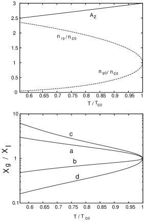
Figure 1: Upper plate: $A_{z}(T)$ in Eq.(3.13), $n_{\ell 0}/n_{c0}$, and $n_{g0}/n_{c0}$ vs $T/T_{c0}$ in the van der Waals theory. Lower plate: ${\cal K}=X_{g}/X_{\ell}$ vs $T/T_{c0}$ in dilute mixtures on a semi-logarithmic scale, where $(r,w)=$ $(0.8,0.8)$ for (a), $(0.8,1.0)$ for (b), $(1.5,1.0)$ for (c), and $(1.5,1.4)$ for (d). Two parameters $r$ and $w$ are defined in Eq.(3.9).

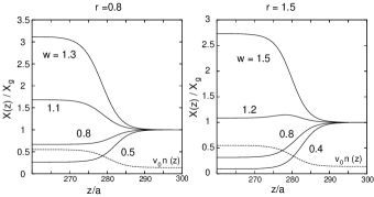
Figure 2: Profiles of the normalized molar fraction $X(z)/X_{g}$ of the solute at $T=0.9T_{c}$ for $r=0.8$ and $w=1.3,1.1,0.8$, and 0.5 (left) and for $r=1.5$ and $w=1.5,1.2,0.8$, and 0.4 (right). It tends to ${\cal K}^{-1}$ on the left hand side. Shown also is the normalized density $v_{0}n(z)$ of the pure fluid composed of the first component (broken line). Space is measured in units of the molecular size $a=v_{10}^{1/3}$.

From Eq.(3.11) the logarithm of the partition coefficient ${\cal K}$ in Eq.(2.24) is expressed as

$$\ln{\cal K}=\frac{(r-1)\Delta\phi}{(1-\phi_{\ell})(1-\phi_{g})}-\frac{2\epsilon}{T}(w-1)\Delta\phi,$$ (3.12)

where $\phi_{\ell}=v_{01}n_{\ell 0}$, $\phi_{g}=v_{01}n_{g0}$, and $\Delta\phi=\phi_{\ell}-\phi_{g}=v_{10}\Delta n$. In the lower plate of Fig.1, $\cal K$ vs $T/T_{c0}$ is shown for typical four cases. Remarkably, the azeotropy (${\cal K}=1$) is attained in the dilute limit on the following line in the $r$-$w$ plane,

$${r-1}=A_{z}(T)({w-1}),$$ (3.13)

where the coefficient $A_{z}(T)$ is determined by the solvent properties only as

$$A_{z}(T)=2(1-\phi_{\ell})(1-\phi_{g})\epsilon/{T}.$$ (3.14)

See the upper plate of Fig.1 for $A_{z}(T)$ vs $T/T_{c0}$. Here $A_{z}\to 3$ as $T\to T_{c0}$, while for $\phi_{g}\ll 1$ we find $A_{z}\cong 2/\phi_{\ell}$ from Eqs.(3.6) and (3.7) and

$$\ln{\cal K}\cong[{r-1}-A_{z}({w-1})]\phi_{\ell}^{2}\epsilon/T.$$ (3.15)

Using $k_{H}$ in Eq.(2.26), Sengers et al.Sengers1 examined $k_{H}/f_{0}$ where $f_{0}=\exp(\mu_{0}/T)$ is the fugacity of the pure fluid. In the van der Waals theory it is of the form,

$$\ln\frac{k_{H}}{f_{0}}=\frac{3}{2}\ln\frac{m_{1}}{m_{2}}+\frac{r-1}{1-\phi_{\ell}}\phi_{\ell}-\frac{2\epsilon}{T}(w-1)\phi_{\ell}.$$ (3.16)

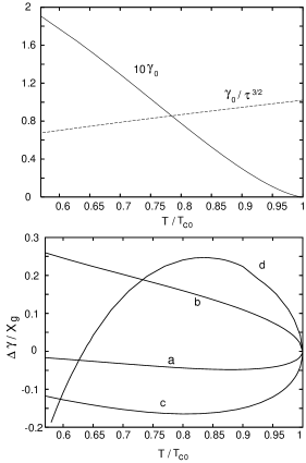
Figure 3: Upper plate: Surface tension $\gamma_{0}$ multiplied by 10 and $\gamma_{0}/\tau^{3/2}$ vs $T/T_{c0}$ for the pure fluid. Lower plate: $\Delta\gamma/X_{g}=-T\Gamma/X_{g}$ vs $T/T_{c0}$ in dilute mixtures, where $(r,w)=$ $(0.8,0.8)$ for (a), $(0.8,1.0)$ for (b), $(1.5,1.0)$ for (c), and $(1.5,1.4)$ for (d). The $\gamma_{0}$ and $\Delta\gamma$ are measured in units of $\epsilon/a^{2}$.

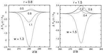
Figure 4: Excess solute density $\Delta n_{2}(z)$ in Eq.(3.17) divided by the molar fraction in the gas $X_{g}$ in units of $v_{10}^{-1}$.

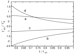
Figure 5: Ratio of the temperature derivatives $\gamma^{\prime}_{\rm cx}=(\partial\gamma/\partial T)_{{\rm cx},p}$ and $\gamma^{\prime}_{0}=d\gamma_{0}/dT$ vs $T/T_{c0}$ in dilute mixtures, where $(r,w)=$ $(0.8,0.8)$ for (a), $(0.8,1.0)$ for (b), $(1.5,1.0)$ for (c), and $(1.5,1.4)$ for (d). It changes its sign for (d).

In Fig.2, we display profiles of the molar fraction $X(z)$ divided by the molar fraction in the gas region $X_{g}$ at $T=0.9T_{c}$, where $A_{z}=2.88$. In the left panel, we set $r=0.8$ and vary $w$ as $1.3,1.1,0.8$, and 0.5. In the right panel, at $r=1.5$, we have $w=1.5,1.2,0.8$, and 0.4. Thus $X_{\ell}/X_{g}={\cal K}^{-1}$ increases with decreasing $r$ and/or with increasing $w$. In our numerical analysis, we set $D_{11}=D_{12}=10a^{5}$ with $a=v_{10}^{1/3}$. See the next subsection for justification of this choice of $D_{11}$. It is worth noting that Sahimi and Taylor calculated the density profiles of two components around an interface Sahimi .

III.3 Surface tension

In the upper plate of Fig.3, we show $\gamma_{0}$ and $\gamma_{0}/\tau^{3/2}$ vs $T/T_{c0}$ for the pure fluid, where we used the formula (A5) in Apenndix A with $D_{11}=10a^{5}$. The relation $\gamma_{0}\propto\tau^{3/2}$ nicely holds over a wide range of $T/T_{c0}$. Remarkably, experimental data of the surface tension of water can also be nicely fitted to the formula $\gamma_{\rm exp}=A_{exp}(1-T/T_{c0})^{3/2}$ over a wide temperature range except close to the criticality (in the range $1-T/T_{c0}\gtrsim 0.1)$ Kie . As in our previous work Kitamura , we have determined $D_{11}$ such that our numerical $\gamma$ and the experimental $\gamma_{\rm exp}$ for water reasonably agree except close to the criticality. In fact, at $T/T_{c}=0.675$, our $\gamma$ is 42.5 dyn$/$cm if we set $D_{11}=10a^{5}$, $a=3{\rm\AA}$, and $T_{c0}=647.1$K, while the experimental value of water is 44.6 dyn$/$cm.

In the lower plate of Fig.3, we display the surface tension change $\Delta\gamma=-T\Gamma$ divided by $X_{g}$ vs $T/T_{c0}$ for four sets of $(r,w)$. From Eq.(2.27) $\Gamma$ is the space integral of the excess solute density $\Delta n_{2}(z)$ expressed in terms of the density $n(z)$ of the reference pure fluid,

$$\Delta n_{2}(z)=n_{2}(z)-n_{2\ell}-\frac{n_{2\ell}-n_{2g}}{n_{\ell 0}-n_{g0}}(n(z)-n_{\ell 0}).$$ (3.17)

In Fig.4, we plot $n_{2}(z)$ for $r=0.8$ (left) and $r=1.5$ (right) for various $w$. With increasing $w$, $\Gamma$ becomes negative and its magnitude increases strongly. In Fig.5, we display the ratio $(dp_{c}/dX)/K_{\rm Kr}=(\partial\gamma/\partial T)_{{\rm cx},p}/(d\gamma/dT)$ calculated from Eq.(2.31) as a function of $T/T_{c0}$ for four sets of $(r,w)$. It even changes its sign from positive to negative with increasing $T$ for $(r,w)=(1.5,1.4)$.

III.4 Near-critical behavior

The Landau expansion of $f_{0}$ with respect to $\psi=n-n_{c0}$ is given in Eq.(2.32). For the van der Waals model the coefficients are given by

$$A_{0}=\frac{27}{4}v_{10},\quad B_{0}=\frac{243}{16}T_{c0}v_{10}^{3}.$$ (3.18)

In the pure fluid, the liquid and gas densities are $n_{\ell 0}=n_{c0}+\psi_{e}$ and $n_{g0}=n_{c0}-\psi_{e}$, where Eq.(2.49) gives

$$\psi_{e}=2n_{c0}\tau^{1/2}.$$ (3.19)

Here $\tau=1-T/T_{c0}$ is the reduced temperature (positive below the critical temperature). See the upper plate of Fig.1 for $n_{\ell 0}$ and $n_{g0}$. Then,

$$\Delta n=2\psi_{e},\quad\Delta v=18v_{10}^{2}\psi_{e},\quad\Delta s=9v_{10}\psi_{e}.$$ (3.20)

These differences are of order $\tau^{1/2}$. In particular, $\Delta s=6\tau^{1/2}$. The latter two relations are consistent with the Clausius-Clapeyron relation $\Delta s/\Delta v=(\partial p/\partial T)_{\rm cx}=1/2v_{10}$ along the coexistence curve. In addition, the correlation length $\xi$ in Eq.(2.51) becomes $\xi=0.86a\tau^{-1/2}$ in our numerical analysis with $D_{11}=10a^{5}$.

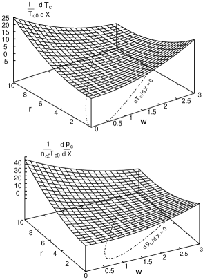
Figure 6: $T_{c0}^{-1}dT_{c}/dX$ (upper plate) and $(n_{c0}T_{c0})^{-1}dp_{c}/dX$ (lower plate) as functions of $r$ and $w$ in Eq.(3.9) near the solvent critical point.

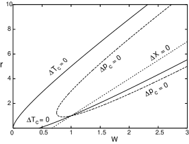
Figure 7: Curves of $\Delta T_{c}=0$, $\Delta p_{c}=0$, and $\Delta X=0$ on the plane of $(r,w)$ near the solvent critical point.

Using $\varphi$ in Eq.(3.6) we perform the Taylor expansion $e^{-\varphi}=C_{0}+C_{1}\psi+C_{2}\psi^{2}/2+\cdots$ as in Eq.(2.36). In terms of $r$ and $w$ in Eq.(3.9) the coefficients are expressed as

$$C_{0} = \frac{2}{3}\exp(-r/2+9w/4),$$

$$C_{1} = \frac{3}{4}v_{10}(-3r-2+9w)C_{0},$$

$$C_{2} = \frac{81}{16}v_{10}^{2}[(r-3w)^{2}-4w]C_{0}.$$ (3.21)

The critical solute density and concentration are

$$n_{2c}=C_{0}\zeta,\quad X_{c}=3v_{10}C_{0}\zeta.$$ (3.22)

The solute density difference in Eq.(2.18) and the composition difference in Eq.(2.19) are expressed as

$${\Delta n_{2}}=(3r-9w+2)X_{c}n_{c0}\tau^{1/2},$$

$$\Delta X=3(r-3w+2)X_{c}\tau^{1/2}.$$ (3.23)

The Krichevskii parameter in Eq.(2.47) is given by

$$K_{\rm Kr}/n_{c0}T_{c0}=\frac{3}{4}(r-3w+2),$$ (3.24)

which was already derived by Petsche and Debenedetti De . See Table 1 for experimental values of the above quantity. In accord with these results, ${\cal K}$ behaves as

$${\cal K}=1+3(r-3w+2)\tau^{1/2}+\cdots.$$ (3.25)

while $\ln(k_{H}/f_{0})={\rm const.}+3(r-3w+2)\tau^{1/2}/2+\cdots$ from Eq.(3.16). Sengers et al. Sengers1 found that data of $T\ln(k_{H}/f_{0})$ can well be fitted to the form $C+B(n_{\ell}-n_{c0})$ near the critical point for a number of solutes in H₂O.

From Eqs.(2.43) and (2.44) the derivatives $dT_{c}/dX$ and $dp_{c}/dX$ along the critical line are written as

$$\frac{1}{T_{c0}}\frac{dT_{c}}{dX}=\frac{1}{4}(r-3w)^{2}-w,$$ (3.26)

$$\frac{1}{p_{c0}}\frac{dp_{c}}{dX}=(r-3w)(r-3w+2)-4(w-1).$$ (3.27)

In Fig. 6, we show $dT_{c}/dX$ and $dp_{c}/dX$ in the $r$-$w$ plane. In Fig.7, we show the curves of $dT_{c}/dX=0$, $dp_{c}/dX=0$, and the azeotropic line $\Delta X=0$. Thus, $\Delta X$, $dT_{c}/dX$, and $dp_{c}/dX$ can be both positive and negative depending on $r$ and $w$.

From Eqs.(2.58) and (3.26) the surface adsorption $\Gamma$ is written as

$$\Gamma=\frac{1}{4}[(r-3w)^{2}-4w]X_{c}\frac{d\gamma_{0}}{dT}.$$ (3.28)

From Eq.(2.60) we calculate the temperature-derivative of $\gamma$ on the coexistence surface,

$${\bigg{(}}\frac{\partial{\gamma}}{\partial{T}}{\bigg{)}}_{{\rm cx},p}=\bigg{[}\frac{r-3w}{2}-\frac{2(w-1)}{r-3w+2}\bigg{]}\frac{d\gamma_{0}}{dT}.$$ (3.29)

Thus the above derivative can be both negative and positive and can even diverge to $\pm\infty$ on the azeotropic line $r-3w+2=0$.

IV Summary

In summary, a Ginzburg-Landau theory has been presented for dilute binary mixtures, where the solute-solvent interaction is relevant but the solute-solute interaction is negligible. A parameter $\zeta$ proportional to the solute fugacity has been introduced in Eq.(2.8). Up to first order in $\zeta$, all the physical quantities of binary mixtures can easily be calculated in terms of the properties of the one-component fluid and the solute-solvent interaction parameters. In more detail, our main results are as follows
(i) The coexistence surface has been given by Eqs.(2.16) and (2.23) or by Eq.(2.22). Henry’s constants have been introduced in Eqs.(2.24)-(2.26).
(ii) The Gibbs formula for the surface tension change $\Delta\gamma$ in Eq.(2.27) has been derived in Appendix A. The surface tension derivative $(\partial\gamma/\partial T)_{p{\rm cx}}$ with respect to $T$ at fixed $p$ has been obtained in Eq.(2.31). Interestingly, it consists of two terms both being independent of $\zeta$.
(iii) The critical temperature shift $\Delta T_{c}$ is given in Eq.(2.41) and the critical pressure shift $\Delta p_{c}$ in Eq.(2.42).
(iv) The Krichevskii parameter $K_{\rm Kr}$ has been given in Eqs.(2.47) and (2.48). The normalized parameter $K_{\rm Kr}X_{c}/n_{c0}T_{c0}$ represents the size of the critical concentration fluctuations as in Eq.(2.49), leading to Eq.(2.52).
(v) The surface adsorption $\Gamma$ has been realted to $\Delta T_{c}$ as in Eq.(2,58) and $(\partial\gamma/\partial T)_{{\rm cx},p}$ to $\Delta p_{c}$ as in Eq.(2,66) near the criticality. The solute effect on the near-critical surface tension is simply to shift the critical temperature $T_{c0}$ by $\Delta T_{c}$ as in Eq.(2.59).
(vi) Experimental data of $dT_{c}/dX$, $dp_{c}/dX$, and $K_{\rm Kr}$ have been given in scaled forms in Table 1, which shows that they can be both positive and negative.
(vii) The van der Waals model of binary mixtures has given simple expressions for all the theoretical expressions in Section II, as illustrated in the figures. The solute-solvent interaction is described in terms of the size ratio $r$ and the potential ratio $w$ in Eq.(3.9).
(viii) The profiles of the solute density and its excess near an interface have been numerically calculated as in Fig. 2 and 4. The negative adsorption becomes marked for large $w$.
(ix) The near-critical behavior in the van der Waals model is very simple in the mean-field theory. In terms of $r$ and $w$ we have calculated $\cal K$, $K_{\rm Kr}$, $dT_{c}/dX$, $dp_{c}/dX$, $\Gamma$, and $(\partial\gamma/\partial T)_{{\rm cx},p}$. In the $r$-$w$ plane , we have plotted $dT_{c}/dX$ and $dp_{c}/dX$ in Fig.6 and the curves of $dT_{c}/dX=0$, $dp_{c}/dX=0$, and ${\cal K}=1$ in Fig. 7.

Finally, we propose measurements of the surface tension as a function of the temperature in the isobaric condition for various solutes in water or in CO₂. From our theory, the derivative $(\partial\gamma/\partial T)_{{\rm cx}.p}$ becomes independent of the solute density in the dilute limit and can be both negative and positive, being delicately dependent on the size ratio $r$ and the potential ratio $w$ in the van der Waals theory as in Eq.(3.29). It is a relevant parameter determining the Marangoni flow around a bubble moving in heat flow in binary mixtures, as will be reported shortly.

Appendix A: Calculation of surface tension

Here the surface tension $\gamma$ of binary mixtures is examined from Eq.(2.1). The grand potential density of mixtures is given by

$$\omega=f-\sum_{i}\hat{\mu}_{i}n_{i}+\frac{T}{2}\sum_{i,j}D_{ij}n_{i}^{\prime}n_{j}^{\prime},$$ (A1)

where $n_{i}^{\prime}=dn_{i}/dz$ and $\hat{\mu}_{i}$ take the values in two-phase coexistence. All the quantities change along the $z$ axis. The space integral of $\omega$ gives the grand potential $\Omega$ in Eq.(2.10). Then $\omega$ tends to $-p_{\rm cx}$ far from the interface $z\to\pm\infty$ and the surface tension is expressed as

$$\gamma=\int dz[\omega(z)+p_{\rm cx}].$$ (A2)

Differentiation of $\omega(z)$ in Eq.(A1) with respect to $z$ yields $d\omega/dz=2T\sum_{ij}D_{ij}n_{i}^{\prime}n_{j}^{\prime\prime}$ from Eq.(2.6), where $n_{j}^{\prime\prime}=d^{2}n_{j}/dz^{2}$. Therefore,

$$\omega = T\sum_{ij}D_{ij}n_{i}^{\prime}n_{j}^{\prime}-p_{\rm cx}$$ (A3)

$$= 2(f-\sum_{i}\hat{\mu}_{i}n_{i})+p_{\rm cx}.$$

Then $\gamma$ in Eq.(A2) may also be expressed as $\gamma=\int dzT\sum_{ij}D_{ij}n_{i}^{\prime}n_{j}^{\prime}=2\int dz(f-\sum_{i}\hat{\mu}_{i}n_{i}+p_{\rm cx})$.

Next $\gamma$ is expanded with respect to $\zeta$ in the dilute case. As in the derivation of Eq.(2.11), elimination of $\hat{\mu}_{2}$ in Eq.(A1) gives

$${\gamma}=\int dz\bigg{[}f_{0}(n_{1})-{\hat{\mu_{1}}}n_{1}+p_{\rm cx}+\frac{T}{2}D_{11}n_{1}^{\prime 2}-Tn_{2}\bigg{]},$$ (A4)

where $\hat{\mu}_{1}=\mu_{\rm cx}^{0}+\delta\mu_{1{\rm cx}}$, $n_{2}$ is given by the second line of Eq.(2.9), and the integrand vanishes as $z\to\pm\infty$. Let $n=n(z)$ be the density of the reference pure fluid or $n(z)=\lim_{\zeta\rightarrow 0}n_{1}(z).$ Then $n(z)\to n_{\ell 0}$ ($n_{g0}$) as $z\to-\infty$ ($\infty)$ and we have the interface equation (2.7). As $\zeta\to 0$ the surface tension of the pure fluid is obtained as

$${\gamma_{0}}=\int dz\bigg{[}f_{0}(n)-\mu_{\rm cx}^{0}n+p_{\rm cx}^{0}+\frac{T}{2}{D_{11}}n^{\prime 2}\bigg{]}.$$ (A5)

From Eqs.(A4) and (A5) the surface tension change $\Delta\gamma=\gamma-\gamma_{0}$ for small $\zeta$ is expanded with respect to the deviation $\delta n_{1}(z)=n_{1}(z)-n(z)$ as

$$\Delta\gamma = \int dz\bigg{[}(f_{0}^{\prime}(n)-\mu_{\rm cx}^{0}-TD_{11}n^{\prime\prime})\delta n_{1}$$ (A6)

$$-\delta\mu_{1\rm cx}n+\delta p_{\rm cx}-Tn_{2}\bigg{]}+\cdots,$$

to first order in $\zeta$. Here the first term in the brackets vanishes from Eq.(2.7). Further use of Eqs.(2.16) and (2.17) yields the Gibbs relation in Eq.(2.27).

Appendix B: Correlation-function expressions

We examine the correlation-function expressions for thermodynamic derivatives such as $K_{\rm Kr}$ in Eq,(2.47) and $(\partial X/\partial\Delta)_{pT}$ in Eq.(2.52) in the framework in the book of the present author Onukibook . Equivalent relations for $K_{\rm Kr}$ were already used in the literature OC ; De ; Shock .

The microscopic particle densities are written as

$$\hat{n}_{j}({\mbox{\boldmath$r$}})=\sum_{\ell\in j}\delta({\mbox{\boldmath$r$}}-{\mbox{\boldmath$r$}}_{\ell}),$$ (B1)

where the summation is over the particles of the species $j(=1,2)$ at position ${\mbox{\boldmath$r$}}_{\ell}$. Then $n_{j}=\langle{\hat{n}_{j}}\rangle$, where $\langle{\cdots}\rangle$ denotes the equilibrium average. The pair correlation functions are written as

$$\langle{\delta\hat{n}_{i}({\mbox{\boldmath$r$}})\delta\hat{n}_{j}({\mbox{\boldmath$0$}})}\rangle=n_{i}\delta_{ij}\delta({\mbox{\boldmath$r$}})+n_{i}n_{j}g_{ij}(r),$$ (B2)

where $\delta\hat{n}_{i}({\mbox{\boldmath$r$}})=\hat{n}_{i}({\mbox{\boldmath$r$}})-n_{i}$ $(i=1,2)$ are the density deviations and $g_{ij}(r)$ ($i,j=1,2)$ are the radial distribution functions tending to zero for large separtion $r$. It is convenient to introduce the concentration variable ${\hat{X}}({\mbox{\boldmath$r$}})$ and the number density variable $\hat{n}({\mbox{\boldmath$r$}})$ by

$${\hat{X}}=X+\frac{n_{1}}{n^{2}}\hat{n_{2}}-\frac{n_{2}}{n^{2}}\hat{n_{1}},\quad{\hat{n}}=\hat{n_{1}}+\hat{n_{2}},$$ (B3)

where $\langle{\hat{n}}\rangle=n=n_{1}+n_{2}$ and $\langle{\hat{X}}\rangle=X=n_{2}/n$. We define a fluctuation variance for any space-dependent variables $\hat{A}({\mbox{\boldmath$r$}})$ and $\hat{B}({\mbox{\boldmath$r$}})$ by

$$\langle{\hat{A}:\hat{B}}\rangle=\int d{\mbox{\boldmath$r$}}\langle{(\hat{A}({\mbox{\boldmath$r$}})-\langle{\hat{A}}\rangle)(\hat{B}({\mbox{\boldmath$r$}})-\langle{\hat{B}}\rangle)}\rangle.$$ (B4)

The variances among $\hat{n}$ and $\hat{X}$ may be expressed in terms of the thermodynamic derivatives,

$$\langle{\hat{n}:\hat{n}}\rangle=nT{\bigg{(}}\frac{\partial{n}}{\partial{p}}{\bigg{)}}_{T\Delta},\quad\langle{\hat{X}:\hat{X}}\rangle=\frac{T}{n}{\bigg{(}}\frac{\partial{X}}{\partial{\Delta}}{\bigg{)}}_{pT},$$

$$\langle{\hat{n}:\hat{X}}\rangle=nT{\bigg{(}}\frac{\partial{X}}{\partial{p}}{\bigg{)}}_{T\Delta}=\frac{T}{n}{\bigg{(}}\frac{\partial{n}}{\partial{\Delta}}{\bigg{)}}_{pT},$$ (B5)

where $n$ and $X$ are treated as functions of the field variables $T$, $p$, and $\Delta=\mu_{2}-\mu_{1}$ in the derivatives. These variances are linear combinations of the variances among the densities, which are written as

$$I_{ij}\equiv\langle{\hat{n}_{i}:\hat{n}_{j}}\rangle=n_{i}\delta_{ij}+n_{i}n_{j}\int d{\mbox{\boldmath$r$}}g_{ij}(r),$$ (B6)

from Eq.(B2). On the other hand, the compressibility at constant $X$ is written as

$$K_{TX}=\frac{1}{n}{\bigg{(}}\frac{\partial{n}}{\partial{p}}{\bigg{)}}_{TX}=\frac{1}{n^{2}T}\bigg{[}\langle{\hat{n}:\hat{n}}\rangle-\frac{\langle{\hat{n}:\hat{X}}\rangle^{2}}{\langle{\hat{X}:\hat{X}}\rangle}\bigg{]},$$ (B7)

Near the mixture criticality, the ratio $K_{TX}/K_{T\Delta}$ behaves as $X/\langle{\hat{X}:\hat{X}}\rangle\cong nX/[(\partial X/\partial\Delta)_{Tp}T]$ (see Eq.(2.52)). All the variances in Eqs.(B5) and (B6) diverge strongly at the mixture criticality except for special cases such as the critical azeotropy. In the low density limit $X\to 0$ under Eq.(2.44), Eqs.(B3) and (B6) give

$$\langle{\hat{X}:\hat{X}}\rangle\cong\langle{\hat{n}_{2}:\hat{n}_{2}}\rangle/n^{2}\cong X/n.$$ (B8)

We also need to assume $\langle{\hat{X}:\hat{n}}\rangle\propto X$ for the existence of the Krichevskii parameter (see Eqs.(B9) and (B10)).

We next examine the thermodynamic derivative $({\partial p}/{\partial X})_{nT}=-(\partial{n}/\partial{X})_{pT}/{nK_{TX}}$. Its correlation-function expression reads

$${\bigg{(}}\frac{\partial{p}}{\partial{X}}{\bigg{)}}_{nT}=\frac{-nT\langle{\hat{n}:\hat{X}}\rangle}{\langle{\hat{n}:\hat{n}}\rangle\langle{\hat{X}:\hat{X}}\rangle-\langle{\hat{n}:\hat{X}}\rangle^{2}}.$$ (B9)

In the low density limit we use Eq.(B8) and replace the denominator of Eq.(B9) by $\langle{\hat{n}:\hat{n}}\rangle X/n$ to find

$$\lim_{X\to 0}\frac{1}{nT}{\bigg{(}}\frac{\partial{p}}{\partial{X}}{\bigg{)}}_{nT} = -\lim_{X\to 0}\frac{n\langle{\hat{n}:\hat{X}}\rangle}{X\langle{\hat{n}:\hat{n}}\rangle}$$ (B10)

$$= 1-n_{1}C_{12}^{\infty},$$

where the second line follows from Eq.(B3). We define

$$C_{12}^{\infty}=\lim_{n_{2}\to 0}\langle{\hat{n}_{2}:\hat{n}_{1}}\rangle/n_{2}\langle{\hat{n}_{1}:\hat{n}_{1}}\rangle,$$ (B11)

which coincides with the space-integral of the direct correlation function $C_{12}(r)$ in the dilute limit De ; OC ; Shock . Here we define $C_{ij}(r)$ in dimensionless forms Onukibook . Thus the Krichevskii parameter $K_{\rm Kr}$ in Eq.(2.47) is the value of $n_{1}T(1-n_{1}C_{12}^{\infty})$ at the solvent criticality. This expression has been used to estimate $K_{\rm Kr}$ for given molecular interaction parameters OC ; De ; Shock . From Eqs.(B10) and (B11) the singular parts of $\hat{X}$ and $\hat{n}_{2}$ are

$$(\hat{X})_{\rm sing} = (C_{12}^{\infty}-1/n_{1})X\delta{\hat{n}}_{1},$$

$$(\hat{n}_{2})_{\rm sing} = C_{12}^{\infty}n_{2}\delta{\hat{n}}_{1},$$ (B12)

near the mixture criticality. Here we have calculated projected parts of $\hat{X}$ and ${\hat{n}}_{2}$ onto the critical fluctuation $\delta{\hat{n}}_{1}=\hat{n}_{1}-n_{1}$. Equation (2.52) is then obtained with the aid of Eq.(B8).

Acknowledgments
I would like to thank Dr. J.M.H. Levelt Sengers for informative correspondence on Henry’s law near the criticality. This work was supported by KAKENHI (Grant-in-Aid for Scientific Research) on Priority Area gSoft Matter Physics h from the Ministry of Education, Culture, Sports, Science and Technology of Japan.

References

- (1) S.S. Leung and R.B. Griffiths, Phys. Rev. A 8, 2670 (1973).
- (2) M. A. Anisimov, E. E. Gorodetskii, V. D. Kulikov, and J. V. Sengers, Phys. Rev. E 51, 1199 (1995).
- (3) A. Onuki, Phase Transition Dynamics (Cambridge University Press, Cambridge, 2002).
- (4) M. Japas and J.M.H. Levelt Sengers, AIChE J, 35, 705 (1989); A.H. Harvey and J.M.H. Levelt Sengers, AIChE J, 36, 539 (1990).
- (5) J. M. H. Levelt Sengers, J. of Supercritical Fluids, 4, 215 (1991).
- (6) I. B. Petsche and P. G. Debenedetti, J. Phys. Chem. 95, 386 (1991).
- (7) A.H. Harvey, Ind. Eng. Chem. Res. 37, 3080 (1998).
- (8) J.W. Gibbs, Collected works, vol.1,pp.219-331 (1957), New Haven, CT: Yale University Press.
- (9) J.D. van der Waals: Verhandel. Konink. Acad. Weten. Amsterdam (Sect.1), Vol.1, No.8 (1893), 56 pp. English translation: J.S. Rowlinson: J. Stat. Phys. 20, 197 (1979).
- (10) B. Levich, Physicochemical Hydrodynamics (Prentice-Hall, Englewood Cliffs, N.J., 1962).
- (11) J. Straub, Experimental thermal fluid science, 9, 253 (1994).
- (12) We consider droplet motion in heat flow. For slow motions the pressure deviation is homogeneous around a droplet, while the temperature deviation and the chemical potential deviations at the interface are on the coexistence surface. The surface tension deviation is then .
- (13) I.R. Krichevskii, Russ. J. Phys. Chem. 41, 1332 (1967).
- (14) J. P. O fConnell, Fluid Phase Equil. 6, 21 (1981). A.V. Plyasunov, E.L. Shock, and J. P. O fConnell, Fluid Phase Equil. 247, 18 (2004); A.V. Plyasunov, E.L. Shock, J.P. O’Connell, Fluid Phase Equili. 247, 19 (2006).
- (15) A. V. Plyasunov and E. L. Shock, J. of Supercritical Fluids 20, 91 (2001); Fluid Phase Equilibria 222, 19 (2004).
- (16) J.L. Sengers: How fluids unmix: Discoveries by the school of Van der Waals and Kamerlingh Onnes; J.L. Sengers and A.H.M. Levelt, Physics Today 55, 47 (2002).
- (17) A. Onuki, J. Low Temp. Phys. 61, 101 (1985).
- (18) B.S. Carey, L.E. Scriven, and H.T. Davis, AIChE J. 26, 705 (1980).
- (19) M. Sahimi and B.N. Taylor, J. Chem. Phys. 95, 6749 (1991).
- (20) You-Xiang Zuo and E.H. Stenby, Fluid Phase Equilibria, 132, 139 (1997).
- (21) S. B. Kiselev and J. F. Ely, J. Chem. Phys. 119, 8645 (2003).
- (22) S.A. Safran, Statistical Thermodynamics of Surfaces, Interfaces, and Membranes (Addison Wesley, Reading, MA, 1994).
- (23) A. Onuki, J. Chem. Phys. 128, 224704 (2008).
- (24) A.I. Abdulagatov, G.V. Stepanov, and I.M. Abdulagatov, High Temp. 3, 408 (2007).
- (25) M. G. Rabezkii, A. R. Bazaev, I. M. Abdulagatov, J. W. Magee, and E. A. Bazaev, J. Chem. Eng. Data 46, 1610 (2001).
- (26) A. R. Bazaev , I. M. Abdulagatov, J. W. Magee, E. A. Bazaev, and A. E. Ramazanova, J. Supercritical Fluids 26, 115 (2003).
- (27) B.A. Wallace and H. Meyer, Phys. Rev. A 5, 953 (1972); H. Meyer and L.H. Cohen, Phys. Rev. A 38, 2081 (1988).
- (28) H. Kitamura and A. Onuki, J. Chem. Phys. 123, 124513 (2005).