Time’s Barbed Arrow:
Irreversibility, Crypticity, and Stored Information

Abstract

We show why the amount of information communicated between the past and future—the excess entropy—is not in general the amount of information stored in the present—the statistical complexity. This is a puzzle, and a long-standing one, since the latter is what is required for optimal prediction, but the former describes observed behavior. We layout a classification scheme for dynamical systems and stochastic processes that determines when these two quantities are the same or different. We do this by developing closed-form expressions for the excess entropy in terms of optimal causal predictors and retrodictors—the $\epsilon$-machines of computational mechanics. A process’s causal irreversibility and crypticity are key determining properties.

Constructing a theory can be viewed as our attempt to extract from measurements a system’s hidden organization. This suggests a parallel with cryptography whose goal [1] is to not reveal internal correlations within an encrypted data stream, even though it contains, in fact, a message. This is essentially the circumstance that confronts a scientist when building a model for the first time.

In this view, the now-long history in nonlinear dynamics to reconstruct models from time series [2, 3] concerns the case of self-decoding in which the information used to build a model is only that available in the observed process. That is, no “side-band” communication, prior knowledge, or disciplinary assumptions are allowed. Nature speaks for herself only through the data she willingly gives up.

Here we show that the parallel is more than metaphor: building a model corresponds directly to decrypting the hidden state information in measurements. The results show why predicting and modeling are, at one and the same time, distinct and intimately related. Along the way, a number of persistent confusions about the role of (and different kinds of) information in prediction and modeling are clarified. We show how to measure the degree of hidden information and, along the way, identify a new kind of statistical irreversibility that plays a key role.

Any process ${\rm P}(\overleftarrow{{X}},\overrightarrow{{X}})$ is a communication channel: It transmits information from the past $\overleftarrow{{X}}=\ldots{X}_{-3}{X}_{-2}{X}_{-1}$ to the future $\overrightarrow{{X}}={X}_{0}{X}_{1}{X}_{2}\ldots$ by storing it in the present. Here ${X}_{t}$ is the random variable for the measurement outcome at time $t$. Our goal is also simply stated: We wish to predict the future using information from the past. At root, a prediction is probabilistic, specified by a distribution of possible futures $\overrightarrow{{X}}$ given a particular past ${\overleftarrow{{x}}}$: ${\rm P}(\overrightarrow{{X}}|{\overleftarrow{{x}}})$. At a minimum, a good predictor needs to capture all of the information $I$ shared between past and future: ${\bf E}=I[\overleftarrow{{X}};\overrightarrow{{X}}]$—the process’s excess entropy [4, and references therein].

Consider now the goal of modeling—to build a representation that not only allows good prediction, but also expresses the mechanisms that produce a system’s behavior. To build a model of a structured process (a channel), computational mechanics [5] introduced an equivalence relation ${\overleftarrow{{x}}}\sim{\overleftarrow{{x}}}^{\prime}$ to group all histories that give rise to the same prediction—resulting in a map from pasts to the causal states: $\epsilon({\overleftarrow{{x}}})=\{{\overleftarrow{{x}}}^{\prime}:{\rm P}(\overrightarrow{{X}}|{\overleftarrow{{x}}})={\rm P}(\overrightarrow{{X}}|{\overleftarrow{{x}}}^{\prime})\}$. A process’s causal states, $\bm{\mathcal{S}}={\rm P}(\overleftarrow{{X}},\overrightarrow{{X}})/\sim$, partition the space ${\overleftarrow{\rm{\bf{X}}}}$ of pasts into sets that are predictively equivalent. The set of causal states can be discrete, fractal, or continuous. State-to-state transitions are denoted by matrices $T_{\mathcal{S}\mathcal{S}^{\prime}}^{(x)}$ whose elements give the probability of transitioning from one state $\mathcal{S}$ to the next $\mathcal{S}^{\prime}$ on seeing measurement value ${x}$. The resulting model, consisting of the causal states and transitions, is called the process’s $\epsilon$-machine.

Causal states have the Markovian property that they render the past and future statistically independent; they shield the future from the past [5]: ${\rm P}(\overleftarrow{{X}},\overrightarrow{{X}}|\mathcal{S})={\rm P}(\overleftarrow{{X}}|\mathcal{S}){\rm P}(\overrightarrow{{X}}|\mathcal{S})$. In this way, the causal states give a structural decomposition of the process into conditionally independent modules. Moreover, they are optimally predictive [5] in the sense that knowing which causal state a process is in is just as good as having the entire past: ${\rm P}(\overrightarrow{{X}}|\mathcal{S})={\rm P}(\overrightarrow{{X}}|\overleftarrow{{X}})$. In other words, causal shielding is equivalent to the fact [5] that the causal states capture all of the information shared between past and future: $I[\mathcal{S};\overrightarrow{{X}}]={\bf E}$.

Out of all optimally predictive models $\bm{\widehat{{\cal R}}}$—for which $I[\widehat{{\cal R}};\overrightarrow{{X}}]={\bf E}$—the $\epsilon$-machine captures the minimal amount of information that a process must store in order to communicate all of the excess entropy from the past to the future. This is the statistical complexity [5]: ${C_{\mu}}\equiv H[\mathcal{S}]\leq H[\widehat{{\cal R}}]$. In short, ${\bf E}$ is the information transmission rate of the process, viewed as a channel, and ${C_{\mu}}$ is the sophistication of that channel.

In addition to ${\bf E}$ and ${C_{\mu}}$, another key (and historically prior) invariant for dynamical systems and stochastic processes is the entropy rate ${h_{\mu}}$ which is the per-measurement rate at which the process generates information—its degree of intrinsic randomness [6]. Importantly, the $\epsilon$-machine  immediately gives two of these three important invariants: a process’s rate (${h_{\mu}}$) of producing information and the amount (${C_{\mu}}$) of historical information it stores in doing so.

To date, ${\bf E}$ cannot be as directly calculated or estimated as the entropy rate and the statistical complexity. This is truly unfortunate, since excess entropy, and related mutual information quantities, are widely used diagnostics for processes, having been applied to detect the presence of organization in dynamical systems [8, 7, 3, 2], in spin systems [9, 10], in neurobiological systems [11, 12], and even in language, to mention only a few applications. For example, in natural language the excess entropy appears to diverge as ${\bf E}\propto L^{1/2}$, reflecting the long-range and strongly nonergodic organization necessary for human communication [13, 14].

This state of affairs has been a major impediment to understanding the relationships between modeling and predicting and, more concretely, the relationships between (and even the interpretation of) a process’s basic invariants—${h_{\mu}}$, ${C_{\mu}}$, and ${\bf E}$. Here we clarify these issues by deriving explicit expressions for ${\bf E}$ in terms of the $\epsilon$-machine, providing a unified information-theoretic analysis of general processes.

The above development of $\epsilon$-machines concerns using the past to predict the future. But what about retrodicting, using the future to retrodict the past? Usually, one thinks of successive measurements occurring as time increases. Now, consider scanning the measurement variables not in the forward time direction, but in the reverse. The computational mechanics formalism is essentially unchanged, though its meaning and notation need to be augmented.

With this in mind, the previous mapping from pasts to causal states is denoted $\epsilon^{+}$ and it gave, what we will call, the predictive causal states ${\bm{\mathcal{S}}}^{+}$. When scanning in the reverse direction, we have a new relation, $\overrightarrow{{x}}\sim^{-}\overrightarrow{{x}}^{\prime}$, which groups futures that are equivalent for the purpose of retrodicting the past: $\epsilon^{-}(\overrightarrow{{x}})=\{\overrightarrow{{x}}^{\prime}:{\rm P}(\overleftarrow{{X}}|\overrightarrow{{x}})={\rm P}(\overleftarrow{{X}}|\overrightarrow{{x}}^{\prime})\}$. It gives the retrodictive causal states ${\bm{\mathcal{S}}}^{-}={\rm P}(\overleftarrow{{X}},\overrightarrow{{X}})/\sim^{-}$. And, not surprisingly, we must also distinguish a process’s forward-scan $\epsilon$-machine ${M}^{+}$ from its reverse-scan $\epsilon$-machine ${M}^{-}$. They assign corresponding entropy rates, $h_{\mu}^{+}$ and $h_{\mu}^{-}$, and statistical complexities, $C_{\mu}^{+}\equiv H[{\mathcal{S}}^{+}]$ and $C_{\mu}^{-}\equiv H[{\mathcal{S}}^{-}]$, respectively, to the process.

Now we are in a position to ask some questions. Perhaps the most obvious is, In which time direction is a process most predictable? The answer is that a stationary process is equally predictable in either [5]: $h_{\mu}^{-}=h_{\mu}^{+}$. Somewhat surprisingly, though, the effort involved in doing so is not the same [15]: $C_{\mu}^{-}\neq C_{\mu}^{+}$. Naturally, ${\bf E}$ is mute on this score, since the mutual information $I$ is symmetric in its variables [4].

The relationship between predicting and retrodicting a process, and ultimately ${\bf E}$’s role, requires teasing out how the states of the forward and reverse $\epsilon$-machines capture information from the past and the future. To do this we must analyze a four-variable mutual information: $I[\overleftarrow{{X}};\overrightarrow{{X}};{\mathcal{S}}^{-};{\mathcal{S}}^{+}]$. A large number of expansions of this quantity are possible. A systematic development follows from Ref. [16] which showed that Shannon entropy $H[\cdot]$ and mutual information $I[\cdot;\cdot]$ form a measure over the space of events.

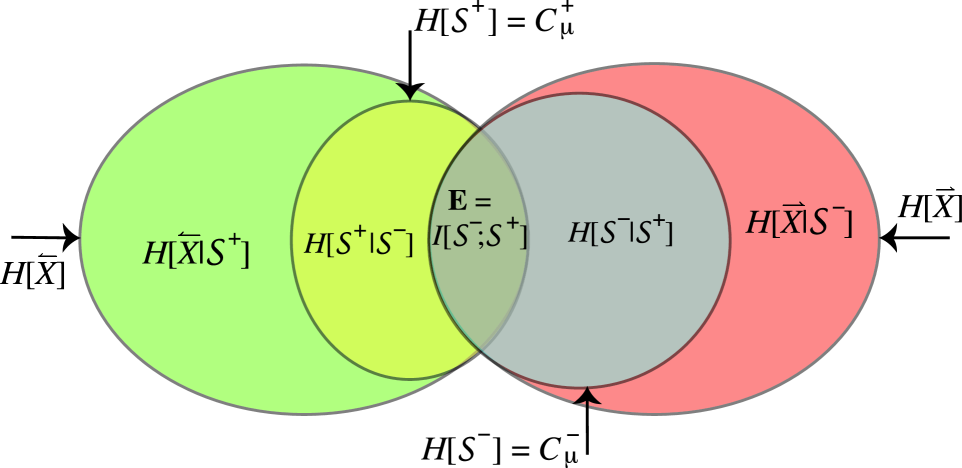
Figure 1: $\epsilon$-Machine information diagram for stationary hidden stochastic processes.

Using an information diagram expansion, it turns out there are 15 possible relationships to consider for $I[\overleftarrow{{X}};\overrightarrow{{X}};{\mathcal{S}}^{-};{\mathcal{S}}^{+}]$. Fortunately, this greatly simplifies in the case of using an $\epsilon$-machine to represent a process: There are only five relationships. (See Fig. 1.) Simplified in this way, we are left with our main results which, due to the preceding effort, are particularly transparent.

Theorem 1.

Excess entropy is the mutual information between the predictive and retrodictive causal states:

$${\bf E}=I[{\mathcal{S}}^{-};{\mathcal{S}}^{+}]~{}.$$ (1)

Notably, the process’s channel capacity ${\bf E}=I[\overleftarrow{{X}};\overrightarrow{{X}}]$ is the same as that of the “channel” between the forward and reverse $\epsilon$-machine states. Moreover, the predictive statistical complexity is given by $C_{\mu}^{+}={\bf E}+H[{\mathcal{S}}^{+}|{\mathcal{S}}^{-}]$ and the retrodictive statistical complexity by $C_{\mu}^{-}={\bf E}+H[{\mathcal{S}}^{-}|{\mathcal{S}}^{+}]$.

Theorem 1 and its two companion results give an explicit connection between a process’s excess entropy and its causal structure—its $\epsilon$-machines. More generally, the relationships directly tie mutual information measures of observed sequences to a process’s structure. They will allow us to probe the properties that control how closely observed statistics reflect a process’s internal hidden structure; that is, the degree to which observed behavior directly reflects internal state information.

At this point we have two separate $\epsilon$-machines, one for predicting and one for retrodicting. We will now show that one can do better, by combining causal information from the past and future. Consider scanning a realization, $\overleftrightarrow{{x}}={\overleftarrow{{x}}}_{t}\overrightarrow{{x}}_{t}$, of the process in the forward direction—seeing histories ${\overleftarrow{{x}}}_{t}$ and noting the series of causal states ${\mathcal{S}}^{+}_{t}=\epsilon^{+}({\overleftarrow{{x}}}_{t})$. Now change direction. What reverse causal state is one in? This is ${\mathcal{S}}^{-}=\epsilon^{-}(\overrightarrow{{x}}_{t})$. We describe the process of changing scan direction with the bidirectional machine ${M}^{\pm}$, which is given by the equivalence relation ${\sim}^{\pm}$:

$$\epsilon^{\pm}(\overleftrightarrow{{x}}) =\epsilon^{\pm}({\overleftarrow{{x}}},\overrightarrow{{x}})$$

$$=\{({{\overleftarrow{{x}}}}^{\prime},{\overrightarrow{{x}}}^{\prime}):{{\overleftarrow{{x}}}}^{\prime}\in\epsilon^{+}({\overleftarrow{{x}}})~{}\mathrm{and}~{}{\overrightarrow{{x}}}^{\prime}\in\epsilon^{-}(\overrightarrow{{x}})\}$$

and has causal states ${\bm{\mathcal{S}}}^{\pm}={\rm P}(\overleftarrow{{X}},\overrightarrow{{X}})/{\sim}^{\pm}\subset{\bm{\mathcal{S}}}^{+}\times{\bm{\mathcal{S}}}^{-}$. That is, the bidirectional causal state the process is in at time $t$ is ${\mathcal{S}}^{\pm}_{t}=(\epsilon^{+}({\overleftarrow{{x}}}_{t}),\epsilon^{-}(\overrightarrow{{x}}_{t}))$. The amount of stored information needed to optimally predict and retrodict a process is ${M}^{\pm}$’s statistical complexity: $C_{\mu}^{\pm}\equiv H[{\mathcal{S}}^{\pm}]=H[{\mathcal{S}}^{-},{\mathcal{S}}^{+}]$.

From the immediately preceding results we obtain the following simple, useful relationship: ${\bf E}=C_{\mu}^{+}+C_{\mu}^{-}-C_{\mu}^{\pm}$. This suggests a wholly new interpretation of the excess entropy—in addition to the original three reviewed in Ref. [4]: ${\bf E}$ is exactly the difference between these statistical complexities. Moreover, only when ${\bf E}=0$ does $C_{\mu}^{\pm}=C_{\mu}^{+}+C_{\mu}^{-}$. The bidirectional machine is also efficient: $C_{\mu}^{\pm}\leq C_{\mu}^{+}+C_{\mu}^{-}$. And we have the bounds: $C_{\mu}^{+}\leq C_{\mu}^{\pm}$ and $C_{\mu}^{-}\leq C_{\mu}^{\pm}$. These results say that taking into account causal information from the past and the future is more efficient than ignoring one or the other and than ignoring their relationship.

We noted above that predicting and retrodicting may require different amounts of information storage ($C_{\mu}^{+}\neq C_{\mu}^{-}$). It is helpful to use causal irreversibility to measure this asymmetry [15]: $\Xi\equiv C_{\mu}^{+}-C_{\mu}^{-}$. With the above results, however, we see that $\Xi=H[{\mathcal{S}}^{+}|{\mathcal{S}}^{-}]-H[{\mathcal{S}}^{-}|{\mathcal{S}}^{+}]$. Note that irreversibility is also not controlled by ${\bf E}$, as the latter is scan-symmetric.

The relationship between excess entropy and statistical complexity established by Thm. 1 indicates that there are fundamental limitations on the amount of a process’s stored information ($C_{\mu}^{\pm}$) directly present in observations (${\bf E}$). We now introduce a measure of this: A process’s crypticity is $d({M}^{+},{M}^{-})\equiv H[{\mathcal{S}}^{+}|{\mathcal{S}}^{-}]+H[{\mathcal{S}}^{-}|{\mathcal{S}}^{+}]$. This is the distance between a process’s forward and reverse $\epsilon$-machines and expresses most explicitly the difference between prediction and modeling. To see this, we need the following connection.

Corollary 1.

${M}^{\pm}$’s statistical complexity is:

$$C_{\mu}^{\pm}={\bf E}+d({M}^{+},{M}^{-})~{}.$$ (2)

Referring to $d$ as crypticity derives from this result: It is the amount of internal state information ($C_{\mu}^{\pm}$) not directly present in the observed sequence (${\bf E}$). That is, a process hides $d$ bits of information.

If crypticity is low ($d\approx 0$), then much of the stored information is present in observed behavior: ${\bf E}\approx C_{\mu}^{\pm}$. However, when a process’s crypticity is high, $d\approx C_{\mu}^{\pm}$, then little of it’s structural information is directly present in observations. Moreover, there are truly cryptic processes (${\bf E}\approx 0$) that are highly structured ($C_{\mu}^{\pm}\gg 0$). Little or nothing can be learned from measurements about such processes’s hidden organization.

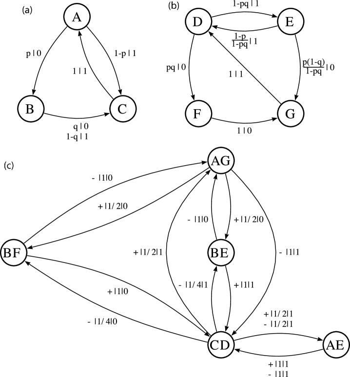
Figure 2: Forward and reverse $\epsilon$-machines for the RIP: ${M}^{+}$ (a) and ${M}^{-}$ (b). Edge labels $t|x$ give the transition probabilities $t=T_{\mathcal{S}\mathcal{S}^{\prime}}^{(x)}$. The bidirectional machine ${M}^{\pm}$ (c) for $p=q=1/2$. Edge labels here prepend the scan direction $\{-,+\}$.

The $\epsilon$-machine information diagram of Fig. 1 encapsulates all of these results concisely. The diagram shows the key relationships between information production ($H[\overrightarrow{{X}}|{\mathcal{S}}^{-}]$ and $H[\overleftarrow{{X}}|{\mathcal{S}}^{+}]$), excess entropy (${\bf E}=I[\overleftarrow{{X}};\overrightarrow{{X}}]$), and stored information ($C_{\mu}^{+}$ and $C_{\mu}^{-}$). Analyzing the $4$-variable information diagram showed that there are only four convex sets of interest. These are depicted as differently shaded ellipses. $H[\overleftarrow{{X}}]$ and $H[\overrightarrow{{X}}]$ (two largest ellipses) are the entropies of the past and future, respectively, which are the process’s total information production. The information stored in the predictive $\epsilon$-machine ${M}^{+}$ is its statistical complexity: $C_{\mu}^{+}\equiv H[{\mathcal{S}}^{+}]$ (small ellipse on left); likewise for ${M}^{-}$, $C_{\mu}^{-}\equiv H({\mathcal{S}}^{-})$ (small ellipse on right). The excess entropy ${\bf E}$ is the intersection of these sets; while the statistical complexity $C_{\mu}^{\pm}$ of the bidirectional machine ${M}^{\pm}$ is their union; the crypticity $d({M}^{+},{M}^{-})$, their symmetric difference; and their signed difference, the causal irreversibility $\Xi$.

Consider an example that illustrates the typical process—cryptic and causally irreversible. This is the random insertion process (RIP) which generates a random bit with bias $p$. If that bit was a $1$, then it outputs another $1$. If the random bit was a $0$, however, it inserts another random bit with bias $q$, followed by a $1$.

Its forward $\epsilon$-machine, see Fig. 2(a), has three recurrent causal states ${\bm{\mathcal{S}}}^{+}=\{A,B,C\}$ and the transition matrices given there. Figure 2(b) gives ${M}^{-}$ which has four recurrent causal states ${\bm{\mathcal{S}}}^{-}=\{D,E,F,G\}$. We see that the $\epsilon$-machines are not the same and so the RIP is causally irreversible. A direct calculation gives ${\rm P}({\mathcal{S}}^{+})={\rm P}(A,B,C)=(1,p,1)/(p+2)$ and ${\rm P}({\mathcal{S}}^{-})={\rm P}(D,E,F,G)=(1,1-pq,pq,p)/(p+2)$. If $p=q=1/2$, for example, these give us $C_{\mu}^{+}\approx 1.5219$ bits, $C_{\mu}^{-}\approx 1.8464$ bits, and ${h_{\mu}}=3/5$ bits per measurement. The causal irreversibility is $\Xi\approx 0.3245$ bits.

Let’s analyze its bidirectional machine; shown in Fig. 2(c) for $p=q=1/2$. The interdependence between the forward and reverse states is given by:

$$\Pr({\mathcal{S}}^{+},{\mathcal{S}}^{-})=\frac{1}{(p+2)(1-pq)}$$

$$\times\bordermatrix{&D&E&F&G\cr A&0&0&pq(1-p)&p(1-pq)\cr B&0&(1-pq)^{2}&p^{2}q(1-q)&0\cr C&1-pq&0&0&0}~{}.$$

By way of demonstrating the exact analysis now possible, ${\bf E}$’s closed-form expression for the RIP family is

$${\bf E}=\log_{2}(p+2)-\frac{p\log_{2}p}{p+2}-\frac{1-pq}{p+2}H\left(\frac{1-p}{1-pq}\right)~{},$$

where $H(\cdot)$ is the binary entropy function. The first two terms on the RHS are $C_{\mu}^{+}$ and the last is $H[{\mathcal{S}}^{+}|{\mathcal{S}}^{-}]$.

Setting $p=q=1/2$, one calculates that ${\rm P}({\mathcal{S}}^{\pm})={\rm P}(AE,AG,BE,BF,CD)=\left(1/5,1/5,1/10,1/10,2/5\right)$. This and the joint distribution give $C_{\mu}^{\pm}=H[{\mathcal{S}}^{\pm}]\approx 2.1219$ bits, but an ${\bf E}=I[{\mathcal{S}}^{+};{\mathcal{S}}^{-}]=1.2464$ bits. That is, the excess entropy (the apparent information) is substantially less than the statistical complexities (stored information)—a rather cryptic process: $d\approx 0.8755$ bits.

To close, the main results establish that when $d>0$ one cannot simply use sequence information directly to represent a process as storing ${\bf E}$ bits of information. We must instead store ${C_{\mu}}$ bits of information, building a causal model of the hidden state information. Why? Because typical processes encrypt their state information within their observed behavior. More precisely, observed information can be arbitrarily small (${\bf E}\approx 0$) compared to the stored information (${C_{\mu}}$).

In deriving an explicit relationship between excess entropy and the $\epsilon$-machine, the framework puts prediction on an equal footing with modeling and so allows for a direct comparison between them. Also, as we demonstrated with the RIP example, it gives a way to develop closed-form expressions for ${\bf E}$. Finally and most generally, it reveals an intimate connection between unpredictability, irreversibility, crypticity, and information storage.

Practically, the results clear up persistent confusions in several literatures that conflate observed (mutual) information and a process’s stored information. Analyzing a process only in terms of mutual information misses an arbitrarily large amount of a process’s structure. When this happens, one concludes that a process is more random than it is and that it has little structure, when neither is true.

Chris Ellison was partially supported on a GAANN fellowship. The Network Dynamics Program funded by Intel Corporation also partially supported this work.

References

- [1] C. E. Shannon. Bell Sys. Tech. J., 28:656–715, 1949.
- [2] H. Kantz and T. Schreiber. Nonlinear Time Series Analysis. Cambridge University Press, Cambridge, UK, second edition, 2006.
- [3] J. C. Sprott. Chaos and Time-Series Analysis. Oxford University Press, Oxford, UK, second edition, 2003.
- [4] J. P. Crutchfield and D. P. Feldman. CHAOS, 13(1):25–54, 2003.
- [5] J. P. Crutchfield and K. Young. Phys. Rev. Let., 63:105–108, 1989; J. P. Crutchfield and C. R. Shalizi, Phys. Rev. E 59(1) 275–283 (1999).
- [6] C. E. Shannon. Bell Sys. Tech. J., 27:379–423, 623–656, 1948.
- [7] M. Casdagli and S. Eubank, editors. Nonlinear Modeling, Reading, Massachusetts, 1992. Addison-Wesley.
- [8] A. Fraser and H. L. Swinney. Phys. Rev. A, 33:1134–1140, 1986.
- [9] J. P. Crutchfield and D. P. Feldman. Phys. Rev. E, 55(2):1239R–1243R, 1997.
- [10] I. Erb and N. Ay. J. Stat. Phys., 115:967–994, 2004.
- [11] G. Tononi, O. Sporns, and G. M. Edelman. Proc. Nat. Acad. Sci. USA, 91:5033–5037, 1994.
- [12] W. Bialek, I. Nemenman, and N. Tishby. Neural Computation, 13:2409–2463, 2001.
- [13] W. Ebeling and T. Poschel. Europhys. Lett., 26:241–246, 1994.
- [14] L. Debowski. IEEE Trans. Info. Th., submitted, 2008.
- [15] J. P. Crutchfield. in Ref. [7]:317–359.
- [16] R. Yeung. IEEE Trans. Info. Th., 37(3):466–474, 1991.