Opportunistic Communications in Fading Multiaccess Relay Channels

Abstract

The problem of optimal resource allocation is studied for ergodic fading orthogonal multiaccess relay channels (MARCs) in which the users (sources) communicate with a destination with the aid of a half-duplex relay that transmits on a channel orthogonal to that used by the transmitting sources. Under the assumption that the instantaneous fading state information is available at all nodes, the maximum sum-rate and the optimal user and relay power allocations (policies) are developed for a decode-and-forward (DF) relay. With the observation that a DF relay results in two multiaccess channels, one at the relay and the other at the destination, a single known lemma on the sum-rate of two intersecting polymatroids is used to determine the DF sum-rate and the optimal user and relay policies. The lemma also enables a broad topological classification of fading MARCs into one of three types. The first type is the set of partially clustered MARCs where a user is clustered either with the relay or with the destination such that the users waterfill on their bottle-neck links to the distant receiver. The second type is the set of clustered MARCs where all users are either proximal to the relay or to the destination such that opportunistic multiuser scheduling to one of the receivers is optimal. The third type consists of arbitrarily clustered MARCs which are a combination of the first two types, and for this type it is shown that the optimal policies are opportunistic non-waterfilling solutions. The analysis is extended to develop the rate region of a $K$-user orthogonal half-duplex MARC. Finally, cutset outer bounds are used to show that DF achieves the capacity region for a class of clustered orthogonal half-duplex MARCs.

I Introduction

Node cooperation in multi-terminal wireless networks has been shown to improve performance by providing increased robustness to channel variations and by enabling energy savings (see [1, 2, 3, 4, 5, 6, 7] and the references therein). A specific example of relay cooperation in multi-terminal networks is the multi-access relay channel (MARC). The MARC is a network in which several users (source nodes) communicate with a single destination with the aid of a relay [8]. The coding strategies developed for the relay channel [9] extend readily to the MARC [10]. For example, the strategy of [9, Theorem 1], now often called decode-and-forward (DF), has a relay that decodes user messages before forwarding them to the destination [3, 11]. Similarly, the strategy in [9, Theorem 6], now often called compress-and-forward (CF), has the relay quantize its output symbols and transmit the resulting quantized bits to the destination [10].

We consider a MARC with a half-duplex wireless relay that transmits and receives in orthogonal channels. Specifically, we model a MARC with a half-duplex relay as an orthogonal MARC in which the relay receives on a channel over which all the sources transmit, and transmits to the destination on an orthogonal channel. This channel models a relay-inclusive uplink in a variety of networks such as wireless LAN, cellular, and sensor networks. The study of wireless relay channels and networks has focused on several performance aspects, including capacity [9, 3, 1], diversity [2, 4, 13], outage [14, 15, 16], and cooperative coding [17, 18]. Equally pertinent is the problem of resource allocation in fading wireless channels where both source and relay nodes can allocate their transmit power to enhance a desired performance metric when the fading state information is available. Resource allocation for a variety of relay channels and networks has been studied in several papers, including [5, 19, 20, 21, 14]. A common assumption in all these papers is that the source and relay nodes are subject to a total power constraint.

For a wireless fading relay channel, i.e., a single-user specialization of a fading MARC, the problem of resource allocation when the source and relay nodes are subject to individual power constraints in studied in [6] (see also [22]). The authors formulate the problem as a max-min optimization. They draw parallels with the classical minimax optimization in hypothesis testing to show that, depending on the joint fading statistics, the resource allocation problem results in one of three solutions. The three solutions broadly correspond to three types of channel topologies, namely, source-relay clustering, relay-destination clustering, and the non-clustered (arbitrary) topology.

Resource allocation in multiuser relay networks has been studied recently in [23, 24, 25]. The authors in [23] and [25] consider a specific orthogonal model where the sources time-duplex their transmissions and are aided in their transmissions by a half-duplex relay, while in [24] the optimal multiuser scheduling is determined under the assumption of a non-fading backhaul channel between the relay and destination. In contrast, in this paper, we consider a more general multiaccess channel with a half-duplex relay and model all inter-node wireless links as ergodic fading channels with perfect fading information available at all nodes. Assuming a DF relay, we develop the optimal source and relay power allocations and present the conditions under which opportunistic time-duplexing of the users is optimal.

The orthogonal MARC is a multiaccess generalization of the orthogonal relay channel studied in [6]; however, the optimal DF policies developed in [6] do not extend readily to maximize the DF sum-rate of the MARC. This is because unlike the single-user case, in order to determine the DF sum-rate for the MARC, we need to consider the intersection of the two multiaccess rate regions that result from decoding at both the relay and the destination. Here, we exploit the polymatroid properties of these multiaccess regions and use a single known lemma on the sum-rate of two intersecting polymatroids [26, chap. 46] to develop inner (DF) and outer bounds on the sum-rate and the rate region and specify the sub-class of orthogonal MARCs for which the DF bounds are tight.

A lemma in [26, chap. 46] enables us to classify polymatroid intersections broadly into two sets, namely, the sets of active and inactive cases. An active or an inactive case result when, in the region of intersection, the constraints on the $K$-user sum-rate at both receivers are active or inactive, respectively. In the sequel we show that inactive cases suggest partially clustered topologies where a subset of users is clustered closer to one of the receivers while the complementary subset is closer to the remaining receiver. On the other hand, active cases can result from specific clustered topologies such as those in which all sources and the relay are clustered or those in which the relay and the destination are clustered, or more generally, from arbitrarily clustered topologies that are either a combination of the two clustered models or of a clustered and a partially clustered model. For both the active and inactive cases, the polymatroid intersection lemma yields closed form expressions for the sum-rates which in turn allow one to develop the sum-rate optimal power allocations (policies).

We first study the two-user orthogonal MARC and develop the DF sum-rate maximizing power policies. Using the polymatroid intersection lemma we show that the fading-averaged DF sum-rate is achieved by either one of five disjoint cases, two inactive and three active, or by a boundary case that lies at the boundary of an active and an inactive case. We develop the sum-rate for all cases and show that the sum-rate maximizing DF power policy either: 1) exploits the multiuser fading diversity to opportunistically schedule users analogously to the fading MAC [27, 28] though the optimal multiuser policies are not necessarily water-filling solutions, or 2) involves simultaneous water-filling over two independent point-to-point links. Using similar techniques, we also develop the two-user DF rate region.

Next, we generalize the two-user sum-rate and rate region analysis to the $K$-user channel and show that the inactive, active, and boundary cases correspond to partially clustered, clustered, and arbitrarily clustered topologies, respectively. Finally, we develop the cutset outer bounds on the sum-capacity of an ergodic fading orthogonal and non-orthogonal $K$-user Gaussian MARC. We show that DF achieves the sum-capacity for a class of half-duplex MARCs in which the sources and relay are clustered such that the outer bound on the $K$-user sum-rate at the destination dominates all other sum-rate outer bounds. We also show that DF achieves the capacity region when the cutset bounds at the destination are the dominant bounds for all rate points on the boundary of the outer bound rate region.

In the course of developing the main results of this paper, we also show that DF achieves the capacity region of a class of degraded discrete memoryless and Gaussian non-fading orthogonal MARCs where the received signal at the destination is physically degraded with respect to that at the relay conditioned on the transmit signal at the relay. The relatively few capacity results known for specific classes of full-duplex single-user relay channels, such as those for degraded relay channels [9, Theorem 5] and for a class of orthogonal relay channels [12], have not been straightforward to extend to the MARC. The result developed here is the first in which the entire capacity region is given for a class of degraded MARCs. In contrast, in [29] it is shown that DF achieves the sum-capacity of a class of full-duplex degraded Gaussian MARCs for which the polymatroid intersections at the relay and destination belong to the active set.

The paper is organized as follows. In Section II, we present the channel models and introduce polymatroids and a lemma on their intersections. In Section III we develop the DF rate region for ergodic fading orthogonal MARCs. In Section IV we develop the power policies that maximize the DF sum-rate for a two-user MARC. We extend the analysis to the $K$-user orthogonal MARC as well as to non-orthogonal models in Section V. In Section VII, we present outer bounds and illustrate our results numerically. We summarize our contributions in Section VIII.

II Channel Model and Preliminaries

II-A Orthogonal Half-Duplex MARC

A $K$-user MARC consists of $K$ source nodes numbered $1,2,\ldots,K$, a relay node $r\,$,  and a destination node $d$. We write $\mathcal{K}=\left\{1,2,\ldots,K\right\}$ to denote the set of sources, $\mathcal{T}=\mathcal{K}\cup\left\{r\right\}$ to denote the set of transmitters, and $\mathcal{D}=\left\{r,d\right\}$ to denote the set of receivers. In an orthogonal MARC, the sources transmit to the relay and destination on one channel, say channel 1, while the half-duplex relay transmits to the destination on an orthogonal channel 2 as shown in Fig. 1. Thus, a fraction $\theta$ of the total bandwidth resource is allocated to channel 1 while the remaining fraction $\overline{\theta}$ $=$ $1-\theta$ is allocated to channel 2. In the fraction $\theta$, the source $k$, for all $k\in\mathcal{K}$, transmits the signal $X_{k}$ while the relay and the destination receive $Y_{r}$ and $Y_{d,1}$ respectively. In the fraction $\overline{\theta}$, the relay transmits $X_{r}$ and the destination receives $Y_{d,2}$ where the sources precede the relay in the transmission order. In each symbol time (channel use), we thus have

$$\begin{array}[c]{cc}Y_{r}=\sum_{k=1}^{K}H_{r,k}X_{k}+Z_{r},&\end{array}$$ (2)

$$\begin{array}[c]{cc}Y_{d,1}=\sum_{k=1}^{K}H_{d,k}X_{k}+Z_{d,1},&\text{and}\end{array}$$ (4)

$$\begin{array}[c]{cc}Y_{d,2}=H_{d,r}X_{r}+Z_{d,2},&\end{array}$$ (6)

where $Z_{r},$ $Z_{d,1},$ and $Z_{d,2}$ are independent circularly symmetric complex Gaussian noise random variables with zero means and unit variances. We write $H$ to denote a vector of fading gains, $H_{k,m}$, for all $k$ $\in$ $\mathcal{D}$ and $m$ $\in$ $\mathcal{T}$, $k$ $\not=$ $m$, such that $h$ is a realization for a given channel use of a jointly stationary and ergodic (not necessarily Gaussian) fading process $\left\{\underline{H}\right\}$. Note that the channel gains $H_{k,m}$, for all $k,m$, are not assumed to be independent. We assume that the fraction $\theta$ is fixed a priori and is known at all nodes. Since the relay is assumed to be causal, we note that the signal $X_{r}$ at the relay in each channel use depends causally only on the $Y_{r}$ received in the previous channel uses.

Over $n$ uses of the channel, the source and relay transmit sequences $\left\{X_{k,i}\right\}$ and $\left\{X_{r,i}\right\}$, respectively, are constrained in power according to

$$\left.\sum\limits_{i=1}^{n}\left|X_{k,i}\right|^{2}\leq n\overline{P}_{k}\right.,\text{ for all }k\in\mathcal{T}\text{.}$$ (7)

Since the sources and relay know the fading states of the links on which they transmit, they can allocate their transmitted signal power according to the channel state information. We write $P_{k}(\underline{H})$ to denote the power allocated at the $k^{th}$ transmitter, for all $k\in\mathcal{T}$, as a function of the channel states $\underline{H}$. For an ergodic fading channel, (7) then simplifies to

$$\left.\mathbb{E}\left[P_{k}(\underline{H})\right]\leq\overline{P}_{k}\right.\text{ for all }k\in\mathcal{T}$$ (8)

where the expectation in (8) is over the distribution of $H$. We write $\underline{P}\left(\underline{H}\right)$ to denote a vector of power allocations with entries $P_{k}(\underline{H})$ for all $k$ $\in$ ${\mathcal{T}}$, and define $\mathcal{P}$ to be the set of all $\underline{P}\left(\underline{H}\right)$ whose entries satisfy (8). Throughout the sequel, we refer to the fractions $\theta$ and $1-\theta$ as the first and second fractions, respectively.

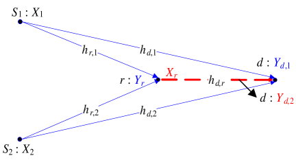
Figure 1: A two-user orthogonal MARC.

II-B Polymatroids

In the sequel, we use the properties of polymatroids to develop the ergodic sum-rate results. Polymatroids have been used to develop capacity characterizations for a variety of multiple-access channel models including the MARC (see for e.g., [30, 28, 11]). Furthermore, in [30], Han demonstrates that for certain multi-terminal channels, polymatroid intersections need to be considered. To the best of our knowledge, this is the first work where the polymatroid intersection lemma has been used to explicitly characterize sum-rates and sum-capacity, where possible. We review the following definition of a polymatroid.

Definition 1

Let $\mathcal{K}=\left\{1,2,\ldots,K\right\}$ and $f=2^{K}\rightarrow\mathfrak{R}_{+}$ be a set function. The polyhedron

$$\mathcal{B}\left(f\right)\equiv\left\{\left(R_{1},R_{2},\ldots,R_{K}\right):R_{\mathcal{S}}\leq f\left(\mathcal{S}\right),\text{ for all }\mathcal{S}\subseteq\mathcal{K}\text{, }R_{k}\geq 0\right\}$$ (9)

is a polymatroid if $f$ satisfies

1. $f\left(\emptyset\right)=0$ (normalization)

2. $f\left(\mathcal{S}\right)\leq f\left(\mathcal{P}\right)$ if $\mathcal{S\subset P}$ (monotonicity)

3. $f\left(\mathcal{S}\right)+f\left(\mathcal{P}\right)\geq f\left(\mathcal{S\cup P}\right)+f\left(\mathcal{S\cap P}\right)$ (submodularity).

Remark 1

The submodularity property in Definition 1 above is equivalent to requiring, for all $k_{1},k_{2}$ in $\mathcal{K}$ with $k_{1}\neq k_{2}$, $k_{1}\notin\mathcal{S}$, $k_{2}\notin\mathcal{S}$, that $f$ satisfies [26, Ch. 44]

$$f(\mathcal{S}\cup\{k_{1}\})+f(\mathcal{S}\cup\{k_{2}\})\geq f(\mathcal{S})+f(\mathcal{S}\cup\{k_{1},k_{2}\}.$$ (10)

This property is used in [11] to show that the rate regions achieved at both the relay and the destination in a full-duplex MARC are polymatroids.

We use the following lemma on polymatroid intersections to develop optimal inner and outer bounds on the sum-rate for $K$-user half-duplex MARCs.

Lemma 1 ([26, p. 796, Cor. 46.1c])

Let $R_{\mathcal{S}}\leq f_{1}\left(\mathcal{S}\right)$ and $R_{\mathcal{S}}\leq f_{2}\left(\mathcal{S}\right)$, for all $\mathcal{S}\subseteq\mathcal{K}$, be two polymatroids such that $f_{1}$ and $f_{2}$ are nondecreasing submodular set functions on $\mathcal{K}$ with $f_{1}\left(\emptyset\right)=f_{2}\left(\emptyset\right)=0$. Then

$$\max R_{\mathcal{K}}=\min\limits_{\mathcal{S}\subseteq\mathcal{K}}\left(f_{1}\left(\mathcal{S}\right)+f_{2}\left(\mathcal{K}\backslash\mathcal{S}\right)\right).$$ (11)

Lemma 1 states that the maximum $K$-user sum-rate $R_{\mathcal{K}}$ that results from the intersection of two polymatroids, $R_{\mathcal{S}}\leq f_{1}\left(\mathcal{S}\right)$ and $R_{\mathcal{S}}\leq f_{2}\left(\mathcal{S}\right)$, is given by the minimum of the two $K$-user sum-rate planes $f_{1}\left(\mathcal{K}\right)$ and $f_{2}\left(\mathcal{K}\right)$ only if both sum-rates are at most as large as the sum of the orthogonal rate planes $f_{1}\left(\mathcal{S}\right)$ and $f_{2}\left(\mathcal{K}\backslash\mathcal{S}\right)$, for all $\emptyset\not=\mathcal{S}\subset\mathcal{K}$. We refer to the resulting intersection as belonging to the set of active cases.

When there exists at least one $\emptyset\not=\mathcal{S}\subset\mathcal{K}$ for which the above condition is not true, an inactive case is said to result. For such cases, the maximum sum-rate in (11) is the sum of two orthogonal rate planes achieved by two complementary subsets of users. As a result, the $K$-user sum-rate bounds $f_{1}(\mathcal{K})$ and $f_{2}(\mathcal{K})$ are no longer active for this case, and thus, the region of intersection is no longer a polymatroid with $2^{K}-1$ faces. For a $K$-user MARC, there are $2^{K}-2$ possible inactive cases.

The intersection of two polymatroids can also result in a boundary case when for any $\mathcal{S\subset K}$, $f_{1}\left(\mathcal{S}\right)+f_{2}\left(\mathcal{K}\backslash\mathcal{S}\right)$ is equal to one or both of the $K$-user sum-rate planes. The orthogonality of the planes $f_{1}\left(\mathcal{S}\right)$ and $f_{2}\left(\mathcal{K}\backslash\mathcal{S}\right)$ implies that no two inactive cases have a boundary and thus a boundary case always arises between an inactive and an active case. Note that by definition, a boundary case is also an active case though for ease of exposition, throughout the sequel we explicitly distinguish between them. From (11), there are three possible active cases corresponding to the three cases in which the sum-rate plane at one of the receivers is smaller than, larger than, or equal to that at the other. In fact, the case in which the sum-rates are equal is also a boundary case between the other two active cases. Thus, there are a total of $\left(2^{K}-1\right)$ boundary cases for each active case.

In summary, the inactive set consists of all intersections for which the constraints on the two sum-rates are not active, i.e., no rate tuple on the sum-rate plane achieved at one of the receivers lies within or on the boundary of the rate region achieved at the other receiver. On the other hand, the intersections for which there exists at least one such rate tuple such that the two sum-rates constraints are active belong to the active set. Thus, by definition, the active set also includes those boundary cases between the active and inactive cases for which there is exactly one such rate pair.

III Two-User Orthogonal MARC: Ergodic DF Rate Region

The DF rate region for a discrete memoryless MARC and a full-duplex relay is developed in [3, Appendix A] (see [11] for a detailed proof). For this model, $X_{k}$, $k\in\mathcal{T}$, denotes the transmit signals at the sources and relay and $Y_{r}$ and $Y_{d}$, denote the received signals at the relay and destination, respectively. The rate region is achieved using block Markov encoding and backward decoding. The following proposition summarizes the DF rate region.

Proposition 1 ([11, Appendix I])

The DF rate region is the union of the set of rate tuples $(R_{1},R_{2},\ldots,$ $R_{K})$ that satisfy, for all $\mathcal{S}\subseteq\mathcal{K}$,

$$R_{\mathcal{S}}\leq\min\left\{I(X_{\mathcal{S}};Y_{r}|X_{\mathcal{S}^{c}}V_{\mathcal{K}}X_{r}U),I(X_{\mathcal{S}}X_{r};Y_{d}|X_{\mathcal{S}^{c}}V_{\mathcal{S}^{c}}U)\right\}$$ (12)

where the union is over all distributions that factor as

$$p(u)\cdot\left({\textstyle\prod\nolimits_{k=1}^{K}}p(v_{k}|u)p(x_{k}|v_{k},u)\right)\cdot p(x_{r}|v_{\mathcal{K}},u)\cdot p(y_{r},y_{d}|x_{\mathcal{T}}).$$ (13)

Remark 2

The time-sharing random variable $U$ ensures that the region of Theorem 1 is convex.

Remark 3

The independent auxiliary random variables $V_{k}$, $k=1,2,\ldots,K$, help the sources cooperate with the relay.

In [10] (see also [31, Proposition 2.5]), the DF rate bounds for a discrete memoryless MARC with a half-duplex relay are developed. For the orthogonal MARC model studied, since the sources and relay transmit on orthogonal channels, the need for auxiliary random variables $V_{k}$, for all $k$, that model the coherent combining gains is eliminated. Under the assumption that the transmit (bandwidth) fractions $\theta$ and $1-\theta$ at the users and relay, respectively, are known at all nodes, the following proposition summarizes the DF rate region for the orthogonal half-duplex MARC.

Proposition 2

The DF rate region of a orthogonal MARC is the union of the set of rate tuples $(R_{1},R_{2},\ldots,$ $R_{K})$ that satisfy, for all $\mathcal{S}\subseteq\mathcal{K}$,

$$R_{\mathcal{S}}\leq\min\left\{\theta I(X_{\mathcal{S}};Y_{r}|X_{\mathcal{S}^{c}}U),\theta I(X_{\mathcal{S}};Y_{d,1}|X_{\mathcal{S}^{c}}U)+\overline{\theta}I(X_{r};Y_{d,2}|U)\right\}$$ (14)

where the union is over all distributions that factor as

$$p(u)\cdot\left(\theta\left[{\textstyle\prod\nolimits_{k=1}^{K}}p(x_{k}|u)\right]\cdot p(y_{r},y_{d}|x_{\mathcal{K}})+\overline{\theta}p(x_{r}|u)\cdot p(y_{d}|x_{r})\right).$$ (15)

Definition 2

A parallel MARC is a collection of $M$ MARCs, for which the inputs and outputs of parallel channel (sub-channel) $j$, $j=1,2,\ldots,M$, are $X_{k,j}$, $k\in\mathcal{K}\cup\left\{r\right\}$ and $\left(Y_{r,j},Y_{d,j}\right)$, respectively, such that conditioned on its inputs, the outputs of each sub-channel are independent of the inputs and outputs of other sub-channels.

Theorem 1

For the parallel MARC, the DF rate region is the union of the set of rate tuples $(R_{1},R_{2},\ldots,$ $R_{K})$ that satisfy, for all $\mathcal{S}\subseteq\mathcal{K}$,

$$R_{\mathcal{S}}\leq\min\left\{\sum\nolimits_{m=1}^{M}I(X_{\mathcal{S},m};Y_{r,m}|X_{\mathcal{S}^{c},m}V_{\mathcal{K},m}X_{r,m}U_{m}),\right.\\ \left.\sum\nolimits_{m=1}^{M}I(X_{\mathcal{S}.,m}X_{r,m};Y_{d,m}|X_{\mathcal{S}^{c},m}V_{\mathcal{S}^{c},m}U_{m})\right\}$$ (16)

where the union is over all distributions that factor as

$${\textstyle\prod\nolimits_{m=1}^{M}}\left(p(u_{m})\cdot{\textstyle\prod\nolimits_{k=1}^{K}}p(v_{k,m},x_{k,m}|u_{m})p(y_{r,m},y_{d,m}|x_{\mathcal{T},m})\right).$$ (17)

Proof:

The inner bounds in (16) are obtained by setting $U=\left(U_{1}\text{ }U_{2}\text{ }\ldots\text{ }U_{M}\right)$, $V_{k}=\left(V_{k,1}\text{ }V_{k,2}\text{ }\ldots\text{ }V_{k,M}\right)$, $X_{k}=\left(X_{k,1}\text{ }X_{k,2}\text{ }\ldots\text{ }X_{k,M}\right)$, $Y_{r}=\left(Y_{r,1}\text{ }Y_{r,2}\text{ }\ldots\text{ }Y_{r,M}\right)$, and $Y_{d}=\left(Y_{d,1}\text{ }Y_{d,2}\text{ }\ldots\text{ }Y_{d,M}\right)$, in (12) and choosing $\left(U_{m},V_{\mathcal{K},m},X_{\mathcal{K},m}\right)$ to be independent for all $m$. ∎

For the (half-duplex) orthogonal Gaussian MARC with a fixed $\underline{H}$ and $\theta$ that is assumed known at all nodes, we consider Gaussian signaling with zero mean and variance $P_{k}$ at transmitter $k$ such that $X_{k}\sim C\mathcal{N}(0,P_{k})$, for all $k\in\mathcal{K}$. Thus, from (14) the DF rate region includes the set of all rate pairs $(R_{1},R_{2})$ that satisfy

$$R_{k}\leq\min\left\{\theta C\left(\frac{\left|H_{d,k}\right|^{2}P_{k}}{\theta}\right)+\overline{\theta}C\left(\frac{\left|H_{d,r}\right|^{2}P_{r}}{\overline{\theta}}\right),\theta C\left(\frac{\left|H_{r,k}\right|^{2}P_{k}}{\theta}\right)\right\},k=1,2$$ (18)

and

$$R_{1}+R_{2}\leq\min\left\{\theta C\left(\sum\limits_{k=1}^{2}\frac{\left|H_{d,k}\right|^{2}P_{k}}{\theta}\right)+\overline{\theta}C\left(\frac{\left|H_{d,r}\right|^{2}P_{r}}{\overline{\theta}}\right),\theta C\left(\sum\limits_{k=1}^{2}\frac{\left|H_{r,k}\right|^{2}P_{k}}{\theta}\right)\right\}.$$ (19)

For a stationary and ergodic process $\left\{\underline{H}\right\}$, the channel in (2)-(6) can be modeled as a set of parallel Gaussian orthogonal MARCs, one for each fading instantiation $\underline{H}$. For a power policy $\underline{P}(\underline{H})$, the DF rate bounds for this ergodic fading channel are obtained from Theorem 1 by averaging the bounds in (18) and (19) over all channel realizations. The ergodic fading DF rate region, $\mathcal{R}_{DF}$, achieved over all $\underline{P}(\underline{H})\in\mathcal{P}$, for a fixed bandwidth fraction $\theta$, is summarized by the following theorem.

Theorem 2

The DF rate region $\mathcal{R}_{DF}$ of an ergodic fading orthogonal Gaussian MARC is

$$\mathcal{R}_{DF}=\bigcup\limits_{\underline{P}\in\mathcal{P}}\left\{\mathcal{R}_{r}\left(\underline{P}\right)\cap\mathcal{R}_{d}\left(\underline{P}\right)\right\}$$ (20)

where, for all $\mathcal{S}\subseteq\mathcal{K}$, we have

$$\mathcal{R}_{r}\left(\underline{P}\right)=\left\{\left(R_{1},R_{2}\right):R_{\mathcal{S}}\leq\mathbb{E}\left[\theta C\left(\frac{\sum\limits_{k\in\mathcal{S}}\left|H_{r,k}\right|^{2}P_{k}(\underline{H})}{\theta}\right)\right]\right\}$$ (21)

and

$$\mathcal{R}_{d}\left(\underline{P}\right)=\left\{\left(R_{1},R_{2}\right):R_{\mathcal{S}}\leq\mathbb{E}\left[\theta C\left(\frac{\sum\limits_{k\in\mathcal{S}}\left|H_{d,k}\right|^{2}P_{k}(\underline{H})}{\theta}\right)+\overline{\theta}C\left(\frac{\left|H_{d,r}\right|^{2}P_{r}(\underline{H})}{\overline{\theta}}\right)\right]\right\}.$$ (22)

Proof:

The proof follows from the observation that the channel in (2)-(6) can be modeled as a set of parallel Gaussian orthogonal MARCs, one for each fading instantiation $\underline{H}$. Thus, from Theorem 1, for Gaussian inputs and for each $\underline{P}(\underline{H})\in\mathcal{P}$, the regions $\mathcal{R}_{r}\left(\underline{P}(\underline{H})\right)$ and $\mathcal{R}_{d}\left(\underline{P}(\underline{H})\right)$ are given by the bounds in (21) and (22), respectively. The DF rate region, $\mathcal{R}_{DF}$, is given by the union of such intersections, one for each $\underline{P}(\underline{H})\in\mathcal{P}$. The convexity of $\mathcal{R}_{DF}$ follows from the convexity of the set $\mathcal{P}$ and the concavity of the $\log$ function. Consider two rate tuples $\left(R_{1}^{\prime},R_{2}^{\prime}\right)$ and $\left(R_{1}^{\prime\prime},R_{2}^{\prime\prime}\right)$ that result from the policies $P$${}^{\prime}(\underline{H})$ and $P$${}^{\prime\prime}(\underline{H})$, respectively. For any $\lambda>0$ such that $\overline{\lambda}=1-\lambda$, and for all $k=1,2$, from (21), we bound $R_{k}=\lambda R_{k}^{\prime}+\left(1-\lambda\right)R_{k}^{\prime\prime}$ achieved at the relay as

$$R_{k} \leq\lambda\theta\mathbb{E}\left[C\left(\frac{\left|H_{r,k}\right|^{2}P_{k}^{\prime}(\underline{H})}{\theta}\right)\right]+\overline{\lambda}\theta\mathbb{E}\left[C\left(\frac{\left|H_{r,k}\right|^{2}P_{k}^{\prime\prime}(\underline{H})}{\theta}\right)\right]$$ (23)

$$\leq\theta\mathbb{E}\left[C\left(\frac{\left|H_{r,k}\right|^{2}\left(\lambda P_{k}^{\prime}(\underline{H})+\overline{\lambda}P_{k}^{\prime\prime}(\underline{H})\right)}{\theta}\right)\right]$$ (24)

$$\leq\theta\mathbb{E}\left[C\left(\frac{\left|H_{r,k}\right|^{2}P_{k}(\underline{H})}{\theta}\right)\right]$$ (25)

where (24) follows from Jensen’s inequality and (25) follows from the convexity of the set $\mathcal{P}$ such that $\underline{P}(\underline{H})=\left(\lambda\underline{P}^{\prime}(\underline{H})+\overline{\lambda}\underline{P}^{\prime\prime}(\underline{H})\right)\in\mathcal{P}$. Thus, we see that the bound on $R_{k}$ is achievable. One can similarly bound the sum-rate $R_{1}+R_{2}$ achieved at the relay thus proving that the tuple $\left(R_{1},R_{2}\right)\in\mathcal{R}_{r}$. The same approach also allows us to show that $\left(R_{1},R_{2}\right)\in\mathcal{R}_{d}$, thus proving that $R_{DF}$ is convex. ∎

Proposition 3

$\mathcal{R}_{r}\left(\underline{P}(\underline{H})\right)$ and $\mathcal{R}_{d}\left(\underline{P}(\underline{H})\right)$ are polymatroids.

Proof:

In [11, Sec. IV.B], it is shown that for each choice of the input distribution in (13), the DF rate region in (12) is an intersection of two polymatroids, one resulting from the bounds at the relay and the other from the bounds at the destination. For the orthogonal MARC, the bounds in (14), relative to (12), involve a weighted sum of mutual information expressions; using the same approach as in [11, Sec. IV.B], the submodularity of these expressions can be verified in a straightforward manner. ∎

Remark 4

The DF rate region given by (18) and (19) is achieved using block Markov encoding at the sources. For the ergodic fading model, the rates in Theorem 2 are obtained assuming that all fading instantiations are seen in each such block.

In the following section, we develop sum-rate optimal DF power policies.

IV Two-User Orthogonal MARC: DF Sum-Rate Optimal Power Policy

For ease of notation, throughout the sequel, we write $R_{\mathcal{A},j}$ to denote the sum-rate bound on the users in $\mathcal{A}$ and $\mathcal{R}_{\mathcal{A},j}^{\min}$ to denote the sum-rate obtained by successively decoding the users in $\mathcal{K}\backslash\mathcal{A}$ before decoding those in $\mathcal{A}$ at receiver $j=r,d$. For the two-user case, $R_{\mathcal{K},j}$ and $R_{\mathcal{A},j}$, for all $\mathcal{A}\subset\mathcal{K}$ are given by the sum-rate and single-user bounds in (21) and (22) at the relay and destination, respectively. The rate $\mathcal{R}_{\mathcal{A},j}^{\min}$ $=$ $R_{\mathcal{K},j}-R_{\mathcal{K}\backslash\mathcal{A},j}$, for all $\mathcal{A}\subset\mathcal{K}$, is obtained by successively decoding the users in $\mathcal{K}\backslash\mathcal{A}$ before decoding those in $\mathcal{A}$ at the corner points of the regions $\mathcal{R}_{r}$ and $\mathcal{R}_{d}$.

The region $\mathcal{R}_{DF}$ in (20) is a union of the intersections of the regions $\mathcal{R}_{r}(\underline{P}(\underline{H}))$ and $\mathcal{R}_{d}(\underline{P}(\underline{H}))$ achieved at the relay and destination respectively, where the union is over all $\underline{P}(\underline{H})\in$ $\mathcal{P}$. Since $\mathcal{R}_{DF}$ is convex, each point on the boundary of $\mathcal{R}_{DF}$ is obtained by maximizing the weighted sum $\mu_{1}R_{1}$ $+$ $\mu_{2}R_{2}$ over all $\underline{P}(\underline{H})\in\mathcal{P}$, and for all $\mu_{1}>0$, $\mu_{2}>0$. Specifically, we determine the optimal policy $\underline{P}^{\ast}(\underline{H})$ that maximizes the sum-rate $R_{1}+R_{2}$ when $\mu_{1}$ $=$ $\mu_{2}$ $=$ $1$. Observe from (20) that every point on the boundary of $\mathcal{R}_{DF}$ results from the intersection of the polymatroids (pentagons) $\mathcal{R}_{r}(\underline{P}(\underline{H}))$ and $\mathcal{R}_{d}(\underline{P}(\underline{H}))$ for some $\underline{P}(\underline{H})$. In Figs. 2 and 3 we illustrate the five possible choices for the sum-rate resulting from such an intersection for a two-user MARC of which two belong to the inactive set and three to the active set.

The inactive set consists of cases $1$ and $2$ in which user $1$ achieves a significantly larger rate at the relay and destination, respectively, than it does at the other receiver; and vice-versa for user $2$. The active set includes cases $3a$, $3b$, and $3c$ shown in Fig. 2 in which the sum-rate at relay $r$ is smaller, larger, or equal, respectively, to that achieved at the destination $d$. The three boundary cases between case $1$ and the three active cases are shown in Fig. 4 while the remaining three between case $2$ and the active cases are shown in Fig. 5. We denote a boundary case as case $\left(l,n\right)$, $l=1,2,$ $n=3a,3b,3c$.

We write $\mathcal{B}_{i}\subseteq\mathcal{P}$ and $\mathcal{B}_{l,n}\subseteq\mathcal{P}$ to denote the set of power policies that achieve case $i$, $i=1,2,3a,3b,3c$, and case $\left(l,n\right)$, $l=1,2$, $n=3a,3b,3c$, respectively. We show in the sequel that the optimization is simplified when the conditions for each case are defined such that the sets $\mathcal{B}_{i}$ and $\mathcal{B}_{l,n}$ are disjoint for all $i,l,$ and $n$, and thus, are either open or half-open sets such that no two sets share a boundary. Observe that cases $1$ and $2$ do not share a boundary since such a transition (see Fig. 2) requires passing through case $3a$ or $3b$ or $3c$. Finally, note that Fig. 3 illustrates two specific $\mathcal{R}_{r}$ and $\mathcal{R}_{d}$ regions for $3a$, $3b$, and $3c$. For ease of exposition, we write $\mathcal{B}_{3}$ $=$ $\mathcal{B}_{3a}\cup\mathcal{B}_{3b}\cup\mathcal{B}_{3c}$, where $\mathcal{B}_{i}$, $i=3a,3b,3c$.

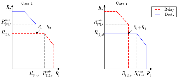
Figure 2: Rate regions $R_{r}(P)$ and $R_{d}(P)$ and sum-rate for case 1 and case 2.

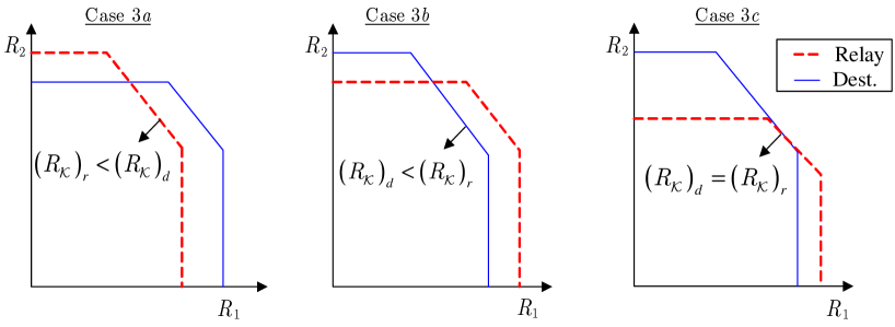
Figure 3: Rate regions $R_{r}(P)$ and $R_{d}(P)$ and sum-rate for cases $3a$, $3b$, and $3c$.

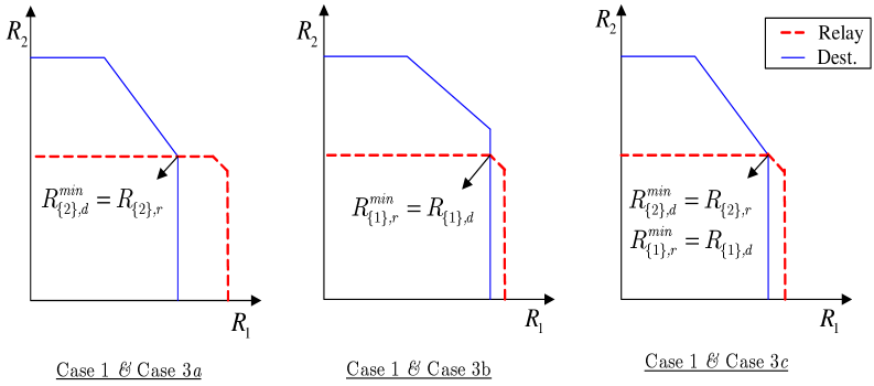
Figure 4: Rate regions $R_{r}(P)$ and $R_{d}(P)$ for cases (1,3a), (1,3b), and (1,3c).

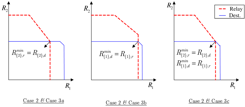
Figure 5: Rate regions $R_{r}(P)$ and $R_{d}(P)$ for cases (2,3a), (2,3b), and (2,3c).

In general, the occurrence of any one of the disjoint cases depends on both the channel statistics and the policy $\underline{P}(\underline{H})$. Since it is not straightforward to know a priori the power allocations that achieve a certain case, we maximize the sum-capacity for each case over all allocations in $\mathcal{P}$ and write $\underline{P}^{(i)}(\underline{H})$ and $\underline{P}^{(l,n)}(\underline{H})$ to denote the optimal solution for case $i$ and case $(l,n)$, respectively. Explicitly including boundary cases ensures that the sets $\mathcal{B}_{i}$ and $\mathcal{B}_{l,n}$ are disjoint for all $i$ and $(l,n)$, i.e., these sets are either open or half-open sets such that no two sets share a power policy in common. This in turn simplifies the convex optimization as follows.

Let $\underline{P}^{(i)}(\underline{H})$ be the optimal policy maximizing the sum-rate for case $i$ over all $\underline{P}(\underline{H})\in\mathcal{P}$. The optimal $\underline{P}^{(i)}(\underline{H})$ must satisfy the conditions for case $i$, i.e., $\underline{P}^{(i)}(\underline{H})\in$ $\mathcal{B}_{i}$. If the conditions are satisfied, we prove the optimality of $P$${}^{\left(i\right)}(\underline{H})$ using the fact that the rate function for each case is concave. On the other hand, when $P$${}^{\left(i\right)}(\underline{H})\not\in$ $\mathcal{B}_{i}$, it can be shown that $R_{1}+R_{2}$ achieves its maximum outside $\mathcal{B}_{i}$. The proof again follows from the fact that $R_{1}+R_{2}$ for all cases is a concave function of $P$$(\underline{H})$ for all $\underline{P}(\underline{H})$ $\in$ $\mathcal{P}$. Thus, when $P$${}^{\left(i\right)}(\underline{H})$ $\not\in$ $\mathcal{B}_{i}$, for every $P$$(\underline{H})\in$ $\mathcal{B}_{i}$ there exists a $P$${}^{\prime}(\underline{H})$ $\in$ $\mathcal{B}_{i}$ with a larger sum-rate. Combining this with the fact that the sum-rate expressions are continuous while transitioning from one case to another at the boundary of the open set $\mathcal{B}_{i}$, ensures that the maximal sum-rate is achieved by some $\underline{P}(\underline{H})$ $\not\in$ $\mathcal{B}_{i}$. Similar arguments justify maximizing the optimal policy for each case over all $\mathcal{P}$. Due to the concavity of the rate functions, only one $\underline{P}^{\left(i\right)}(\underline{H})$ or $\underline{P}^{\left(l,n\right)}(\underline{H})$ will satisfy the conditions for its case. The optimal $\underline{P}^{\ast}(\underline{H})$ is given by this $\underline{P}^{\left(i\right)}(\underline{H})$ or $\underline{P}^{\left(l,n\right)}(\underline{H})$.

The optimization problem for case $i$ or case $\left(l,n\right)$ is given by

(26)

where

(27)

The optimal policy for each case is determined using Lagrange multipliers and the Karush-Kuhn-Tucker (KKT) conditions [32, 5.5.3]. A detailed analysis is developed in the Appendix and we summarize the KKT conditions and the optimal policies for all cases below. From (27), the KKT conditions for each case $x$, $x=i,\left(l,n\right)$, for all $i$ and $\left(l,n\right)$ is given as

$$\begin{array}[c]{cc}f_{k}^{\left(x\right)}\left(\underline{P}(\underline{h})\right)-\nu_{k}\ln 2\leq 0,&\text{with equality for }P_{k}\left(\underline{h}\right)>0\text{, }k=1,2,r\end{array}$$ (28)

where $\nu_{k}$, for all $k=1,2,r$, are dual variables associated with the power constraints in (26). Specializing the KKT conditions for each case, we obtain the optimal policies for each case as summarized below following which we list the conditions that the optimal policy for each case needs to satisfy.

Case $1:$ The functions $f_{k}^{\left(1\right)}\left(\underline{P}(\underline{h})\right)$, $k=1,2,r,$ in (28) for case 1 are

$$\begin{array}[c]{cc}f_{k}^{\left(1\right)}\left(\underline{P}(\underline{h})\right)=\frac{\left|h_{m,k}\right|^{2}}{\left(1+\left|h_{m,k}\right|^{2}\left.P_{k}\left(\underline{h}\right)\right/\theta\right)}&(k,m)=(1,d),(2,r)\text{ }\end{array}$$ (30)

$$\begin{array}[c]{cc}f_{r}^{\left(1\right)}\left(\underline{P}(\underline{h})\right)=\frac{\left|h_{d,r}\right|^{2}}{\left(1+\left|h_{d,r}\right|^{2}\left.P_{k}\left(\underline{h}\right)\right/\overline{\theta}\right)}.&\end{array}$$ (32)

It is straightforward to verify that these KKT conditions simplify to

$$\begin{array}[c]{ll}P_{k}^{\left(1\right)}\left(\underline{h}\right)=\left(\frac{\theta}{\nu_{k}\ln 2}-\frac{\theta}{\left|h_{m,k}\right|^{2}}\right)^{+}&(k,m)=(1,d),(2,r)\end{array}$$ (33)

and

$$P_{r}^{\left(1\right)}\left(\underline{h}\right)=\left(\frac{\overline{\theta}}{\nu_{r}\ln 2}-\frac{\overline{\theta}}{\left|h_{d,r}\right|^{2}}\right)^{+}.\text{ }$$ (34)

Case $2:$ From (27), since $S^{\left(2\right)}$ can be obtained from $S^{\left(1\right)}$ by interchanging the user indexes $1$ and $2$, the functions $f_{k}^{\left(2\right)}\left(\underline{P}(\underline{h})\right)$, and hence, the KKT conditions for this case can be obtained by replacing the superscript $\left(1\right)$ by $\left(2\right)$ and using the pairs $(k,m)=(1,d),(2,r)$ in (30)-(33). The resulting optimal policies are

$$\begin{array}[c]{ll}P_{r}^{\left(2\right)}\left(\underline{h}\right)=P_{r}^{\left(1\right)}\left(\underline{h}\right)&\text{for all }\underline{h}\text{, and}\\ P_{k}^{\left(2\right)}\left(\underline{h}\right)=\left(\frac{\theta}{\nu_{k}\ln 2}-\frac{\theta}{\left|h_{m,k}\right|^{2}}\right)^{+}&(k,m)=(1,r),(2,d).\end{array}$$ (35)

Case $3a:$ The functions $f_{k}^{\left(3a\right)}\left(\underline{P}(\underline{h})\right)$, $k=1,2,$ satisfying the KKT conditions in (28) are

$$\begin{array}[c]{cc}f_{k}^{\left(3a\right)}\left(\underline{P}(\underline{h})\right)=\left|h_{r,k}\right|^{2}\left/\left(1+\sum\limits_{k=1}^{2}\left|h_{r,k}\right|^{2}\left.P_{k}\left(\underline{h}\right)\right/\theta\right)\right.&k=1,2.\end{array}$$ (36)

Since this case maximizes the multiaccess sum-rate at the relay, the optimal user policies are multiuser opportunistic water-filling solutions given by

$$\begin{array}[c]{ll}\frac{\left|h_{r,1}\right|^{2}}{v_{1}}>\frac{\left|h_{r,2}\right|^{2}}{\nu_{2}}&P_{1}^{\left(3a\right)}\left(\underline{h}\right)=\left(\frac{\theta}{\nu_{1}\ln 2}-\frac{\theta}{\left|h_{r,1}\right|^{2}}\right)^{+},P_{2}^{\left(3a\right)}=0\\ \frac{\left|h_{r,1}\right|^{2}}{v_{1}}\leq\frac{\left|h_{r,2}\right|^{2}}{\nu_{2}}&P_{1}^{\left(3a\right)}\left(\underline{h}\right)=0,P_{2}^{\left(3a\right)}=\left(\frac{\theta}{\nu_{2}\ln 2}-\frac{\theta}{\left|h_{r,2}\right|^{2}}\right)^{+}\end{array}$$ (37)

where without loss of generality, the users are time-duplexed even when their scaled fading states in (37) are the same. While the relay power does not explicitly appear in the optimization, since this case results when the sum-rate is smaller than that at the destination, choosing the optimal relay policy to maximize the sum-rate at the destination, i.e., $P_{r}^{\left(3a\right)}\left(\underline{H}\right)=P_{r}^{\left(1\right)}\left(\underline{H}\right)$, suffices.

Case $3b:$ The functions $f_{k}^{\left(3b\right)}\left(\underline{P}(\underline{h})\right)$, $k=1,2,$ satisfying the KKT conditions in (28) can be obtained from (36) by replacing the subscript ‘$r$’ by ‘$d$’ in (36) while $f_{r}^{\left(3b\right)}\left(\underline{P}(\underline{h})\right)=f_{r}^{\left(3a\right)}\left(\underline{P}(\underline{h})\right)=f_{r}^{\left(1\right)}\left(\underline{P}(\underline{h})\right)$. Thus, this case maximizes the multiaccess sum-rate at the destination and the optimal user policies are multiuser opportunistic water-filling solutions given by

$$\begin{array}[c]{ll}\frac{\left|h_{d,1}\right|^{2}}{v_{1}}>\frac{\left|h_{d,2}\right|^{2}}{\nu_{2}}&P_{1}^{\left(3a\right)}\left(\underline{h}\right)=\left(\frac{\theta}{\nu_{1}\ln 2}-\frac{\theta}{\left|h_{d,1}\right|^{2}}\right)^{+},P_{2}^{\left(3a\right)}=0\\ \frac{\left|h_{r,1}\right|^{2}}{v_{1}}\leq\frac{\left|h_{d,2}\right|^{2}}{\nu_{2}}&P_{1}^{\left(3a\right)}\left(\underline{h}\right)=0,P_{2}^{\left(3a\right)}=\left(\frac{\theta}{\nu_{2}\ln 2}-\frac{\theta}{\left|h_{d,2}\right|^{2}}\right)^{+}\end{array}$$ (38)

while the optimal relay policy is a water-filling solution $P_{r}^{\left(3a\right)}\left(\underline{H}\right)=P_{r}^{\left(1\right)}\left(\underline{H}\right)$.

Case $3c:$ The functions $f_{k}^{\left(3c\right)}\left(\underline{P}(\underline{h})\right)$, $k=1,2,r,$ satisfying the KKT conditions in (28) are given as

$$\begin{array}[c]{cc}f_{k}^{\left(3c\right)}\left(\underline{P}(\underline{h})\right)=\left(1-\alpha\right)f_{k}^{\left(3a\right)}\left(\underline{P}(\underline{h})\right)+\alpha f_{k}^{\left(3b\right)}\left(\underline{P}(\underline{h})\right),&k=1,2,\end{array}$$ (40)

$$\begin{array}[c]{cc}f_{r}^{\left(3c\right)}\left(\underline{P}(\underline{h})\right)=\alpha f_{r}^{\left(3b\right)}\left(\underline{P}(\underline{h})\right),&k=r,\end{array}$$ (42)

where the Lagrange multiplier $\alpha$ accounts for the boundary condition

$$R_{\mathcal{K},d}\left(\underline{P}\left(\underline{H}\right)\right)=R_{\mathcal{K},r}\left(\underline{P}\left(\underline{H}\right)\right)$$ (43)

and the optimal policy $\underline{P}^{\left(3b\right)}\left(\underline{H}\right)\in\mathcal{B}_{3c}$ satisfies this condition where $\mathcal{B}_{3c}$ is the set of $\underline{P}\left(\underline{H}\right)$ that satisfy (43). Thus, this case maximizes the multiaccess sum-rate at both the relay and the destination. In the Appendix, using the KKT conditions we show that the optimal user policies are opportunistic in form and are given by

$$\begin{array}[c]{ll}f_{1}^{\left(3c\right)}/\nu_{1}>f_{2}^{\left(3c\right)}/\nu_{2}&P_{1}^{\left(3c\right)}\left(\underline{h}\right)=\left(\text{root of }F_{1}^{\left(3c\right)}|_{P_{2}=0}\right)^{+},P_{2}^{\left(3c\right)}\left(\underline{h}\right)=0\\ f_{1}^{\left(3c\right)}/\nu_{1}\leq f_{2}^{\left(3c\right)}/\nu_{2}&P_{1}^{\left(3c\right)}\left(\underline{h}\right)=0,P_{2}^{\left(3c\right)}\left(\underline{h}\right)=\left(\text{root of }F_{2}^{\left(3c\right)}|_{P_{1}=0}\right)^{+}.\end{array}$$ (44)

Analogous to cases $3a$ and $3b$, the scheduling conditions in (44) depend on both the channel states and the water-filling levels $\nu_{k}$ at both users. However, the conditions in (44) also depend on the power policies, and thus, the optimal solutions are no longer water-filling solutions. In the Appendix we show that the optimal user policies can be computed using an iterative non-water-filling algorithm which starts by fixing the power policy of one user, computing that of the other, and vice-versa until the policies converge to the optimal policy. The iterative algorithm is computed for increasing values of $\alpha\in\left(0,1\right)$ until the optimal policy satisfies (43) at the optimal $\alpha^{\ast}$. The proof of convergence is detailed in the Appendix.

Boundary Cases $\left(l,n\right):$ A boundary case $\left(l,n\right)$ results when

$$\begin{array}[c]{cc}S^{\left(l\right)}=S^{\left(n\right)}&l=1,2,\text{ and }n=3a,3b,3c.\end{array}$$ (45)

Recall that $S^{\left(l\right)}$ and $S^{\left(n\right)}$ are sum-rates for an inactive case $l$, and an active case $n$, respectively. Thus, in addition to the constraints in (26), the maximization problem for these cases includes the additional constraint in (45). For all except the two cases where $n=3c$, the equality condition in (26) is represented by a Lagrange multiplier $\alpha$. The two cases with $n=3c$ have two Lagrange multipliers $\alpha_{1}$ and $\alpha_{2}$ to also account for the condition $S^{\left(3a\right)}=S^{\left(3b\right)}$.

For the different boundary cases, the functions $f_{k}^{\left(l,n\right)}\left(\underline{P}(\underline{h})\right)$, $k=1,2,$ satisfying the KKT conditions in (28) are given as

$$\begin{array}[c]{cc}f_{k}^{\left(l,n\right)}\left(\underline{P}(\underline{h})\right)=\left(1-\alpha\right)f_{k}^{\left(l\right)}\left(\underline{P}(\underline{h})\right)+\alpha f_{k}^{\left(n\right)}\left(\underline{P}(\underline{h})\right),&k=1,2,n\not=3c\end{array}$$ (47)

$$\begin{array}[c]{cc}f_{k}^{\left(l,3c\right)}\left(\underline{P}(\underline{h})\right)=\left(1-\alpha_{1}-\alpha_{2}\right)f_{k}^{\left(l\right)}\left(\underline{P}(\underline{h})\right)+\alpha_{2}f_{k}^{\left(3a\right)}\left(\underline{P}(\underline{h})\right)+\alpha_{1}f_{k}^{\left(3b\right)}\left(\underline{P}(\underline{h})\right),&k=1,2,\end{array}$$ (49)

$$\begin{array}[c]{cc}f_{r}^{\left(l,n\right)}\left(\underline{P}(\underline{h})\right)=\alpha f_{r}^{\left(l\right)}\left(\underline{P}(\underline{h})\right),&n=3a\end{array}$$ (51)

$$\begin{array}[c]{cc}f_{r}^{\left(l,n\right)}\left(\underline{P}(\underline{h})\right)=\alpha f_{r}^{\left(l\right)}\left(\underline{P}(\underline{h})\right)+\left(1-\alpha\right)f_{r}^{\left(n\right)}\left(\underline{P}(\underline{h})\right),&n=3b\end{array}$$ (53)

$$\begin{array}[c]{cc}f_{r}^{\left(l,n\right)}\left(\underline{P}(\underline{h})\right)=\alpha_{1}f_{r}^{\left(l\right)}\left(\underline{P}(\underline{h})\right)+\left(1-\alpha_{1}-\alpha_{2}\right)f_{r}^{\left(3b\right)}\left(\underline{P}(\underline{h})\right),&n=3c\end{array}$$ (55)

For ease of exposition and brevity, we summarize the KKT conditions and the optimal policies for case $\left(1,3a\right)$. In the Appendix, using the KKT conditions we show that the optimal user policies $P_{k}^{\left(1,3a\right)}(\underline{H})$ are opportunistic in form and are given by

$$\begin{array}[c]{ll}\frac{f_{1}^{\left(1,3a\right)}}{\nu_{1}}>\frac{f_{2}^{\left(1,3a\right)}}{\nu_{2}}&P_{1}\left(\underline{h}\right)=\left(\text{root of }F_{1}^{\left(1,3a\right)}|_{P_{2}=0}\right)^{+},P_{2}\left(\underline{h}\right)=0\\ \frac{f_{1}^{\left(1,3a\right)}}{\nu_{1}}\leq\frac{f_{2}^{\left(1,3a\right)}}{\nu_{2}}&P_{1}\left(\underline{h}\right)=0,P_{2}\left(\underline{h}\right)=\left(\text{root of }F_{2}^{\left(1,3a\right)}|_{P_{1}=0}\right)^{+}\end{array}$$ (56)

where $F_{k}^{\left(1,3a\right)}=f_{k}^{\left(1,3a\right)}-\nu_{k}\ln 2,$ $k=1,2.$ As in case $3c$, the optimal policies take an opportunistic non-waterfilling form and in fact can be obtained by an iterative non-water-filling algorithm as described for case $3c$. The optimal $P_{r}^{\left(1,3a\right)}\left(\underline{H}\right)=\alpha P_{r}^{\left(1\right)}\left(\underline{H}\right)$ is a water-filling solution.

The optimal policies for all other boundary cases can be obtained similarly as detailed in the Appendix. In general, for all boundary cases, the optimal user policies are opportunistic non-water-filling solutions while that for the relay are water-filling solutions. Finally, the sum-rate maximizing policy for any case is the optimal policy only if it satisfies the conditions for that case. The conditions for the cases are

$$\begin{array}[c]{cl}\underline{\text{Case}\ 1}:&\begin{array}[c]{ccc}R_{\left\{1\right\},d}<R_{\left\{1\right\},r}^{\min}&\text{and}&R_{\left\{2\right\},r}<R_{\left\{2\right\},d}^{\min}\end{array}\end{array}$$ (59)

$$\begin{array}[c]{cc}\underline{\text{Case}\ 2}:&\begin{array}[c]{ccc}R_{\left\{1\right\},r}<R_{\left\{1\right\},d}^{\min}&\text{and}&R_{\left\{2\right\},d}<R_{\left\{2\right\},r}^{\min}\end{array}\end{array}$$ (62)

$$\begin{array}[c]{cc}\underline{\text{Case}\ 3a}:&\left(R_{\mathcal{K}}\right)_{r}<\left(R_{\mathcal{K}}\right)_{d}\end{array}$$ (64)

$$\begin{array}[c]{cc}\underline{\text{Case}\ 3b}:&\left(R_{\mathcal{K}}\right)_{r}>\left(R_{\mathcal{K}}\right)_{d}\end{array}$$ (66)

$$\begin{array}[c]{cc}\underline{\text{Case}\ 3c}:&\left(R_{\mathcal{K}}\right)_{r}=\left(R_{\mathcal{K}}\right)_{d}\end{array}$$ (68)

$$\begin{array}[c]{cc}\underline{\text{Case}\ \left(1,3a\right)}:&R_{\mathcal{K},r}=R_{\left\{1\right\},d}+R_{\left\{2\right\},r}\text{ }<\left(R_{\mathcal{K}}\right)_{d}\end{array}$$ (70)

$$\begin{array}[c]{cc}\underline{\text{Case}\ \left(2,3a\right)}:&R_{\mathcal{K},r}=R_{\left\{1\right\},r}+R_{\left\{2\right\},d}<\left(R_{\mathcal{K}}\right)_{d}\end{array}$$ (72)

$$\begin{array}[c]{cc}\underline{\text{Case}\ \left(1,3b\right)}:&R_{\mathcal{K},d}=R_{\left\{1\right\},d}+R_{\left\{2\right\},r}<\left(R_{\mathcal{K}}\right)_{r}\end{array}$$ (74)

$$\begin{array}[c]{cc}\underline{\text{Case}\ \left(2,3b\right)}:&R_{\mathcal{K},d}=R_{\left\{1\right\},r}+R_{\left\{2\right\},d}<\left(R_{\mathcal{K}}\right)_{r}\end{array}$$ (76)

$$\begin{array}[c]{cc}\underline{\text{Case}\ \left(1,3c\right)}:&R_{\mathcal{K},r}=R_{\mathcal{K},d}=R_{\left\{1\right\},d}+R_{\left\{2\right\},r}\end{array}$$ (78)

$$\begin{array}[c]{cc}\underline{\text{Case}\ \left(2,3c\right)}:&R_{\mathcal{K},r}=R_{\mathcal{K},d}=R_{\left\{1\right\},r}+R_{\left\{2\right\},d}\end{array}$$ (80)

where in fading state $\underline{H}$, (59)-(80) are evaluated for $X_{k}\sim\mathcal{CN}\left(0,P_{k}^{\left(x\right)}\left(\underline{H}\right)/\theta\right)$, $k=1,2$, and $X_{r}\sim\mathcal{CN}\left(0,P_{r}^{\left(x\right)}\left(\underline{H}\right)/\overline{\theta}\right)$ for $x=i,\left(l,n\right)$.
The following theorem summarizes the form of $P$^∗ and presents an algorithm to compute it.

Theorem 3

The optimal policy $P$${}^{\ast}(\underline{H})$ maximizing the DF sum-rate of a two-user ergodic fading orthogonal MARC is obtained by computing $\underline{P}^{(i)}(\underline{H})$ and $\underline{P}^{(l,n)}(\underline{H})$ starting with the inactive cases $1$ and $2$, followed by the boundary cases $(l,n)$, and finally the active cases $3a,$ $3b,$ and $3c$ until for some case the corresponding $\underline{P}^{(i)}(\underline{H})$ or $\underline{P}^{(l,n)}(\underline{H})$ satisfies the case conditions. The optimal $P$${}^{\ast}(\underline{H})$ is given by the optimal $\underline{P}^{(i)}(\underline{H})$ or $\underline{P}^{(l,n)}(\underline{H})$ that satisfies its case conditions and falls into one of the following three categories:

Inactive Cases: The optimal policy for the two users is such that one user water-fills over its link to the relay while the other water-fills over its link to the destination. The optimal relay policy $P_{r}^{\ast}(\underline{H})$ is water-filling over its direct link to the destination.

Cases $\left(3a,3b,3c\right)$: The optimal user policy $P_{k}^{\ast}(\underline{H})$, for all $k\in\mathcal{K}$, is opportunistic water-filling over its link to the relay for case $3a$ and to the destination for case $3b$. For case $3c$, $P_{k}^{\ast}(\underline{H})$, for all $k\in\mathcal{K}$, takes an opportunistic non-waterfilling form and depends on the channel gains of user $k$ at both receivers. The optimal relay policy $P_{r}^{\ast}(\underline{H})$ is water-filling over its direct link to the destination.

Boundary Cases: The optimal user policy $P_{k}^{\ast}(\underline{H})$, for all $k\in\mathcal{K}$, takes an opportunistic non-water-filling form. The optimal relay policy $P_{r}^{\ast}(\underline{H})$ is water-filling over its direct link to the destination.

Proof:

The closed form expressions for the optimal policies for each case are developed in the Appendix. The need for an order in evaluating $P$${}^{\ast}(\underline{H})$ is due to the following reasons. Since every case results from an intersection of two polymatroids, the conditions in (64)-(68) hold for all cases. Thus, all feasible power policies satisfy one of these three conditions as a result of which these conditions do not allow a clear distinction between the cases. In contrast, the conditions for cases $1$ and $2$ in (59) and (62), respectively, are mutually exclusive. For the boundary cases, since every boundary case $\left(l,n\right)$ results from the intersection of an active case $n=3a,3b,3c,$ with an inactive case $l=1,2,$ and is itself an active case, one of its conditions corresponds to the condition for case $n$, $n=3a,3b$,$3c$ in (64)-(68). Additionally, in the Appendix we show that the boundary condition $S^{\left(l\right)}=S^{\left(n\right)}$ implies that only one of the two inequality conditions of case $l$ holds strictly while the other simplifies to an equality. An immediate implication of these two conditions is that the boundary cases are mutually exclusive and the set of power policies satisfying them are also disjoint from those satisfying cases $1$ and $2$. Thus, to determine the optimal $P$${}^{\ast}(\underline{H})$, one can start with any one of the mutually exclusive inactive and boundary cases. If the optimal policy for any one of these cases satisfies its case conditions, then, $P$${}^{\ast}(\underline{H})$ is given by that policy. However, if all these cases are eliminated, i.e., none of their optimal policies satisfy the appropriate case conditions, the optimal policies for remaining three cases $3a$, $3b$, and $3c$ can be computed one at a time. From (64)-(68), cases $3a$, $3b$, and $3c$ are mutually exclusive, i.e., their feasible power sets are disjoint, and thus, the optimal policy, satisfies the conditions for only one of three active cases. ∎

Remark 5

The conditions for cases $3a$, $3b$, and $3c$ can also be redefined to include the negation of all the conditions for the other cases. This in turn eliminates the need for an order in computing the optimal policy; however, the number of conditions that need to be checked to verify if the optimal policy satisfies the conditions for cases $3a$ or $3b$ or $3c$ remain unchanged relative to the algorithm in Theorem 3.

We now discuss in detail the optimal power policies at the sources and the relay for the different cases.

Optimal Relay Policy: In the orthogonal model we consider, the relay transmits directly to the destination on a channel orthogonal to the source transmissions. Thus, the relay to destination link can be viewed as a fading point to point link. In fact, in all cases the optimal relay policy involves water-filling over the fading states analogous to a fading point to point link (see [33]). However, the exact solution, including scale factors, depends on the case considered.

The optimal cooperation strategy at the relay also depends on the case studied. For instance, consider case $1$ where users 1 and 2 achieve significantly larger rates (relative to the other receiver) at the relay and destination, respectively. Thus, the sum-rate is the sum of the rates achieved over the bottle-neck links from user 1 to the destination and from user 2 to the relay; i.e., it is the sum of the single-user rate user 1 achieves at the destination and the rate user 2 achieves at the relay. The single-user rate achieved by user 1 at the destination requires the relay to completely cooperate with user 1, i.e., the relay uses its power $P_{r}\left(\underline{H}\right)$ to forward only the message from user $1$ in every fading state in which it transmits. As shown in the intersection for case $1$ in Fig. 2, this is due to the fact that since user $1$ achieves a significantly larger rate at the relay than does user $2$, the sum-rate is maximized when the relay allocates its resources entirely to cooperating with user $1$. Finally, for case $2$, the relay cooperates entirely with user $2$.

For the active cases, $3a$ and $3b$, the sum-rate may be achieved by an infinite number of feasible points on one or both of the sum-rate planes; the optimal cooperative strategy at the relay will differ for each such point. Thus, for a corner point the relay transmits a message from only one of the users while for all non-corner points the relay transmits both messages.

For the boundary cases including case $3c$, the requirement of an equality (boundary) condition results in the introduction of an additional parameter. Thus, for case $3c$, the parameter $\alpha$ is introduced to satisfy the equality constraint on the sum-rates achieved at the relay and destination. Similarly for cases $\left(1,3a\right)$, $\left(2,3a\right)$, $\left(1,3b\right)$, and $\left(2,3b\right)$, the parameter $\alpha$ is chosen to ensure that the optimal power policies at the users and relay satisfy the equality constraint for that case. Finally, for cases $\left(1,3c\right)$ and $\left(2,3c\right)$, the requirement of satisfying two boundary conditions requires the introduction of the two parameters, $\alpha_{1}$ and $\alpha_{2}$, one for each condition.

Optimal User Policies: As with the relay, the optimal policies for the two users depend on the case considered. For cases $1$ and $2$, the optimal policies are water-filling solutions, i.e., each user allocates power optimally as if it were transmitting to only that receiver at which it achieves a lower rate. In fact, the conditions for case  1 in (59) suggest a network geometry in which source 1 and the relay are physically proximal enough to form a cluster and source 2 and the destination form another cluster; and vice-versa for case 2. This clustering and the resulting water-filling over the bottle-neck links is the reason why the relay forwards the message of only that user physically proximal to it, namely, only user $1$ and only user $2$ for cases $1$ and $2$, respectively.

For case $3a$, the optimal policies at the two users maximize the sum-rate achieved at the relay (the smaller of sum-rates achieved at the two receivers). These policies are the same as those achieving the sum-capacity of a two-user multiple-access channel with the relay as the intended receiver (see [27, 28]). Thus, the optimal policy for each user involves water-filling over its fading states to the relay. The solution also exploits the multiuser diversity to opportunistically schedule the users in each use of the channel.

Analogously, the optimal policies for case $3b$ require multiuser water-filling over the user links to the destination. For both cases, if the channel gains have a joint fading distribution with a continuous density, the sum-rate maximization simplifies to scheduling only one user in each fading instantiation (parallel channel). Thus, the users time-share their channel use and the maximum sum-rate is achieved by a unique point on the boundary of the rate region (see [28, III.D]).

The optimal policies for case $3c$ require the users to allocate power such that the sum-rates achieved at both the relay and the destination are the same. This constraint has the effect that it preserves the opportunistic scheduling since the sum-rate involves the multiaccess sum-rate bounds at both receivers. However, the solutions are no longer waterfilling due to the fact that the equality (boundary) condition results in the function $f_{k}^{(3c)}$ being a weighted sum of the functions $f_{k}^{(3a)}$ and $f_{k}^{(3b)}$ for cases $3a$ and $3b$, respectively.

Finally, the requirement of satisfying one or more boundary conditions also affects the nature of the optimal policies for all the $\left(l,n\right)$ cases. Thus, for these boundary cases, since the sum-rate planes are active, i.e., the functions $f_{k}^{\left(l,n\right)}$ involve the multiple-access sum-rate bounds, the optimal power policies result in an opportunistic scheduling of the users. However, as with case $3c$, here too the optimal policies are no longer water-filling since the boundary conditions result in the functions $f_{k}^{\left(l,n\right)}$ being weighted sums of the functions for cases $l$ and $n$.

Remark 6

The case conditions in (59)-(80) require averaging over the channel states; thus, the case that maximizes the sum-rate depends on the average power constraints and the channel statistics (including network topology).

Remark 7

The optimal policy for each source for cases $1,$ $2$, $3a$, and $3b$ depends on the channel gains at only one of the receivers. However, the optimal policy for the boundary cases, including case $3c$, depends on the instantaneous channel states at both receivers. Furthermore, all the cases exploiting the multiuser diversity require a centralized protocol to coordinate the opportunistic scheduling of users.

V Two-User DF Rate Region: Optimal Power Policies

In Theorem 2, the DF rate region $\mathcal{R}_{DF}$ is shown to be a union of the intersections of the regions $\mathcal{R}_{r}(\underline{P}(\underline{H}))$ and $\mathcal{R}_{d}(\underline{P}(\underline{H}))$ achieved at the relay and destination, respectively, where the union is over all $\underline{P}(\underline{H})\in$ $\mathcal{P}$. Furthermore, since $\mathcal{R}_{DF}$ is convex, each point on the boundary of $\mathcal{R}_{DF}$ is obtained by maximizing the weighted sum $\mu_{1}R_{1}$ $+$ $\mu_{2}R_{2}$ over all $\underline{P}(\underline{H})\in\mathcal{P}$, and for all $\mu_{1}>0$, $\mu_{2}>0$. In fact, for every $\left(\mu_{1},\mu_{2}\right)$, the rate tuple $\left(R_{1},R_{2}\right)$ that maximizes the weighted sum $\mu_{1}R_{1}+\mu_{2}R_{2}$ results from an intersection of two rate polymatroids.

Thus, analogously to the sum-rate analysis for $\mu_{1}=\mu_{2}=1$, for arbitrary $\left(\mu_{1},\mu_{2}\right)$, $\mu_{1}R_{1}+\mu_{2}R_{2}$, is maximized by either one of two inactive cases, or by one of nine active cases of which six are boundary cases. To find the rate tuple maximizing $\mu_{1}R_{1}+\mu_{2}R_{2}$, we use the classic result in linear programming that the maximum value of a linear function constrained over a feasible bounded polyhedron is achieved at a vertex of the polyhedron [32, Chapter 1.2.2]. Thus, for any $\underline{P}(\underline{H})$, the $\left(R_{1},R_{2}\right)$-tuple maximizing $\mu_{1}R_{1}+\mu_{2}R_{2}$ is given by a vertex of a $\mathcal{R}_{r}\left(\underline{P}(\underline{H})\right)\cap\mathcal{R}_{d}\left(\underline{P}(\underline{H})\right)$ polyhedron at which $\mu_{1}R_{1}+\mu_{2}R_{2}$ is a tangent. Recall that for the two inactive cases, the polymatroid intersections result in rectangles, and thus, there is a unique vertex maximizing $\mu_{1}R_{1}+\mu_{2}R_{2}$. The intersection is also a rectangle for the six boundary cases since these active cases are such that only one point on the sum-rate plane is included in the region of intersection. On the other hand, for cases $3a$, $3b$, and $3c$, the intersection of $K$-dimensional polymatroids results in a $K$-dimensional polyhedron. Thus, for these cases, when $\mu_{1}<\mu_{2}$, $\mu_{1}R_{1}+\mu_{2}R_{2}$ is maximized by that vertex where user $1$ is decoded before user $2$, i.e., at the vertex where user $2$ achieves its maximal single-user rate.

For simplicity, we present the results for cases $1$, $3a$, and $\left(1,3a\right).$ The results for the other cases follow naturally from discussions for these three cases. Without loss of generality, we let $\mu_{1}<\mu_{2}$; the analysis for $\mu_{1}>\mu_{2}$ follows in an analogous manner.

Case 1: From Fig. 2, the weighted sum $\mu_{1}R_{1}+\mu_{2}R_{2}$ for this case is given by

$$\mu_{1}R_{\left\{1\right\},d}+\mu_{2}R_{\left\{2\right\},r}.$$ (81)

Since $\mu_{1}$ and $\mu_{2}$ are independent of the transmit powers, the optimization problem is the same as that for the sum-rate case. Thus, at the maximal rate, users $1$ and $2$ waterfill on their bottleneck links to the destination and relay, respectively.

The analysis for case $2$ is the same as that for case $1$ except now user $1$ and $2$ waterfill on their bottleneck links to the relay and destination, respectively.

Case 3a: The weighted sum $\mu_{1}R_{1}+\mu_{2}R_{2}$ is maximized by the vertex with coordinates

$$R_{1} =R_{\mathcal{K},r}-R_{2}$$ (82)

$$R_{2} =\min\left(R_{\left\{2\right\},r},R_{\left\{2\right\},d}\right).$$ (83)

The maximization of $\mu_{1}R_{1}+\mu_{2}R_{2}$ thus simplifies to

$$\max_{\underline{P}\in\mathcal{P}}\left(\mu_{1}R_{\mathcal{K},r}+\left(\mu_{2}-\mu_{1}\right)\min\left(R_{\left\{2\right\},r},R_{\left\{2\right\},d}\right)\right)$$ (84)

where the optimal $\underline{P}^{\left(3a\right)}(\underline{H})$ satisfies the conditions in (64) for this case. As in the appendix, there are three possible disjoint solutions to the max-min optimization in (84) resulting from either $R_{\left\{2\right\},r}$ being smaller, larger, or equal to $R_{\left\{2\right\},d}$. We discuss the optimal policies for each of these sub-cases separately below.

1. $R_{\left\{2\right\},r}<R_{\left\{2\right\},d}$: For this sub-case, the vertex of interest in (82) and (83) is achieved by the MAC bounds at the same receiver. Thus, the maximization for these cases simplifies to that developed in for an ergodic fading MAC in [28]. The optimal power policies involve water-filling and opportunistic scheduling of the users and water-filling at the relay over its direct link to the destination.

2. $R_{\left\{2\right\},r}>R_{\left\{2\right\},d}$: The maximization here simplifies to

   $$\max_{\underline{P}\in\mathcal{P}}\left(\mu_{1}R_{\mathcal{K},r}+\left(\mu_{2}-\mu_{1}\right)R_{\left\{2\right\},d}\right).$$ (85)

   As with the Lagrangian expressions for the boundary cases in the Appendix, here too, the weighted sum of rates in (85) is an appropriately weighted mixture of sum and single-user rates achieved at the relay and destination, respectively. Thus, analogously to the boundary cases, one can verify in a straightforward manner that the optimal policies maximizing (85) at both users are non-waterfilling solutions with opportunistic scheduling based on relative fading states while that at the relay requires waterfilling over its direct link to the destination. Note that the optimal policies at both the users and the relay depend on the values chosen for $\mu_{1}$ and $\mu_{2}$.

3. $R_{\left\{2\right\},r}=R_{\left\{2\right\},d}$: Subject to average power and positivity constraints, the maximization here simplifies to

   $$\begin{array}[c]{l}\max_{\underline{P}\in\mathcal{P}}\left(\mu_{1}R_{\mathcal{K},r}+\left(\mu_{2}-\mu_{1}\right)R_{\left\{2\right\},r}\right)\\ \text{s.t. }R_{\left\{2\right\},r}=R_{\left\{2\right\},d}.\end{array}$$ (86)

   The maximization in (86) subject to the equality constraint results in a Lagrangian with a weighted mixture of single-user rates achieved at the relay and destination. Thus, the optimal user and relay policies have a form similar to that discussed in the previous sub-case in which the sum-rate and single-user rate are achieved at different receivers,

Remark 8

The three sub-cases for case $3a$ studied above are differentiated by additional constraints relating the single-user rates at the relay and the destination. This in turn implies that the region $\mathcal{B}_{3a}$ will be divided into three mutually exclusive subsets, where the condition for each sub-case is satisfied in only one of the subsets.

Boundary case $\left(1,3a\right)$: Recall that a boundary case $\left(l,n\right)$ results from satisfying the conditions for the active case $n$ and satisfying the conditions for the inactive case $l$ as a mixture of equalities and inequalities. The resulting rate region belongs to the set of active cases but has one unique sum-rate point such that the intersection of pentagons results in a rectangle (see Figs. 4 and 5). Thus, the weighted optimization $\mu_{1}R_{1}+\mu_{2}R_{2}$ for case $\left(1,3a\right)$ simplifies to

$$\begin{array}[c]{l}\mu_{1}R_{\left\{1\right\},d}+\mu_{2}R_{\left\{2\right\},r}\\ \text{s.t. }\left(R_{\mathcal{K}}\right)_{r}=R_{\left\{1\right\},d}+R_{\left\{2\right\},r}.\end{array}$$ (87)

Note that the constraint in (87) is the same as that for the boundary case $\left(1,3a\right)$ in (70). Thus, the constrained maximization problem in (87) is analogous to the sum-rate maximization for the boundary cases and admits a similar non-waterfilling opportunistic solution for the user power policies and a waterfilling solution at the relay.

Remark 9

The discussion here for cases $3a$ and $\left(1,3a\right)$ also applies to the other active (including boundary) cases. In each such case, the optimal policies depend on all the Lagrange dual variables, with each variable reflecting a specific constraint.

VI $K$-User Generalization

VI-A $K$-user Sum-Rate Analysis

We use Lemma 1 to extend the analysis in the previous sections to the $K$-user case. Recall that $\mathcal{R}_{DF}$ is given by a union of the intersection of polymatroids, where the union is over all power policies. From Lemma 1, we have that the maximal $K$-user sum-rate tuple is achieved by an intersection that either belongs to active set or to the inactive set. We write $l=1,2,\ldots,2^{K}-2$, to index the $2^{K}-2$ non-empty subsets of $\mathcal{K}$. For a $K$-user MARC, there are $\left(2^{K}-2\right)$ possible intersections of the inactive kind with sum-rate $J^{\left(l\right)}$ given by

$$\begin{array}[c]{ll}\underline{\text{case}\ l}:S^{\left(l\right)}=R_{\mathcal{S},r}+R_{\mathcal{K}\backslash\mathcal{S},d}&l=1,2,\ldots,2^{K}-2\\ s.t.\text{ }R_{\mathcal{S},r}<R_{\mathcal{S},d}^{\min}\text{ and }R_{\mathcal{K}\backslash\mathcal{S},d}<R_{\mathcal{K}\backslash\mathcal{S},d}^{\min}&\end{array}$$ (88)

where $R_{\mathcal{A},j}$ and $R_{\mathcal{A},j}^{\min}$ are as defined in Section III and for $j=r,d,$ are given by the bounds in (21) and (22), respectively. The sum-rates $J^{\left(i\right)}$, for the active cases $i=3a,3b,3c$, are

$$S^{\left(i\right)} =R_{\mathcal{K},j}\text{ for }\left(i,j\right)=\left(3a,r\right),\left(3b,d\right)$$ (89)

$$S^{\left(3c\right)} =R_{\mathcal{K},r}\text{ }s.t.\text{ }R_{\mathcal{K},r}=R_{\mathcal{K},d}.$$ (90)

Finally, the sum-rate $J^{\left(l,n\right)}$, for the boundary cases totaling $3\left(2^{K}-2\right)$ and enumerated as cases $\left(l,n\right)$, $l=1,2,\ldots,2^{K}-2$, $n=3a,3b,3c$, are

$$\begin{array}[c]{l}\underline{\text{case}~{}\left(l,3a\right)}:S^{\left(l,3a\right)}=R_{\mathcal{K},r}\\ s.t.\text{ }R_{\mathcal{K},r}=R_{\mathcal{S},r}+R_{\mathcal{K}\backslash\mathcal{S},d}\text{ for case }l\end{array}$$ (93)

$$\begin{array}[c]{l}\underline{\text{case}~{}\left(l,3b\right)}:S^{\left(l,3b\right)}=R_{\mathcal{K},d}\\ s.t.\text{ }R_{\mathcal{K},d}=R_{\mathcal{S},r}+R_{\mathcal{K}\backslash\mathcal{S},d}\text{ for case }l\end{array}$$ (96)

$$\begin{array}[c]{l}\underline{\text{case}~{}\left(l,3c\right)}:S^{\left(l,3c\right)}=R_{\mathcal{K},r}\\ s.t.\text{ }R_{\mathcal{K},r}=R_{\mathcal{K},d}=R_{\mathcal{S},r}+R_{\mathcal{K}\backslash\mathcal{S},d}\text{ for case }l\end{array}$$ (99)

where the subset $\mathcal{S}$ is chosen to correspond to the appropriate case $l$.

Remark 10

The constraint for case $l$ in (88) can be obtained directly from the requirement that the $K$-user sum-rate constraints at the two receivers are larger than that for case $l$ (see (11)).

The $K$-user sum-rate optimization problem for cases $i$ and $\left(l,n\right)$ can be written as

(100)

An inactive case $l$ results when the conditions for that case in (88) are satisfied. A boundary case results when the conditions for one of the cases in (93)-(99) is satisfied for the appropriate $\left(l,n\right)$ case. Finally, case $3a$ or $3b$ or $3c$ results when the conditions for neither the inactive nor the boundary cases are satisfied.

As in Section IV, the optimization for each case involves writing the Lagrangian and the KKT conditions. The optimal policy $\underline{P}^{\ast}(\underline{H})$ satisfies the conditions for only one of the cases. For brevity, we summarize the details below.

• Inactive cases: The Lagrangian for these cases involves a sum of the DF bounds at the relay in (21) for users in $\mathcal{S}$, for each non-empty $\mathcal{S}$, and the DF bounds at the destination in (22) for the remaining users in $\mathcal{K}\backslash\mathcal{S}$ such that for $i=1,2,\ldots,2^{K}-2$,

  $$\mathcal{L}^{\left(i\right)} =\mathbb{E}\left[\theta C\left(\sum_{k\in\mathcal{S}}\left|H_{r,k}\right|^{2}\frac{P_{k}(\underline{H})}{\theta}\right)+\theta C\left(\sum_{k\in\mathcal{K}\backslash\mathcal{S}}\left|H_{d,k}\right|^{2}\frac{P_{k}(\underline{H})}{\theta}\right)+\overline{\theta}C\left(\left|H_{d,r}\right|^{2}\frac{P_{r}(\underline{H})}{\overline{\theta}}\right)\right]$$

  $$\text{ \ \ \ \ }-\sum\nolimits_{k\in\mathcal{T}}\nu_{k}\mathbb{E}\left[P_{k}(\underline{H})-\overline{P}_{k}\right]+\sum\nolimits_{k\in\mathcal{T}}\lambda_{k}P_{k}(\underline{H})$$ (101)

  where $\nu_{k}$, for all $k$, are the dual variables associated with the power constraints in (8), and $\lambda_{k}\geq 0$ are the dual variables associated with the positivity constraints ($P_{k}\geq 0$) on $P_{k}$. Writing the KKT conditions, it is straightforward to verify that the optimal policy for a user in $\mathcal{S}$ is a function of the channel gains at the relay while that for a user in $\mathcal{K}\backslash\mathcal{S}$ is a function of the channel gains only at the destination. In fact, when $\mathcal{S}$ or $\mathcal{K}\backslash\mathcal{S}$ are singleton sets, the optimal policy for the user in $\mathcal{S}$ or $\mathcal{K}\backslash\mathcal{S}$ is simply water-filling over its bottle-neck link to either the relay (if $\mathcal{S}$) or the destination (if $\mathcal{K}\backslash\mathcal{S}$). More generally, when $\mathcal{S}$ or $\mathcal{K}\backslash\mathcal{S}$ are not singleton sets, the optimal policy is an opportunistic water-filling solution. Finally, the relay’s policy is water-filling over its direct link to the destination.

• Cases $3a$, $3b$, and $3c$: The Lagrangian for these three cases is given by

  $$\mathcal{L}^{\left(i\right)}=\begin{array}[c]{cc}S^{\left(i\right)}-\sum\nolimits_{k\in\mathcal{T}}\nu_{k}\mathbb{E}\left[P_{k}(\underline{H})-\overline{P}_{k}\right]+\sum\nolimits_{k\in\mathcal{T}}\lambda_{k}P_{k}(\underline{H})&i=3a,3b,3c\end{array}$$ (102)

  where

  $$S^{\left(i\right)}=\left\{\begin{array}[c]{ll}\mathbb{E}\left[\theta C\left(\sum_{k\in\mathcal{K}}\left|H_{r,k}\right|^{2}P_{k}(\underline{H})/\theta\right)\right]&i=3a\\ \mathbb{E}\left[\theta C\left(\sum_{k\in\mathcal{K}}\left|H_{r,k}\right|^{2}P_{k}(\underline{H})/\theta\right)+\overline{\theta}C\left(\left|H_{d,r}\right|^{2}P_{r}(\underline{H})/\overline{\theta}\right)\right]&i=3b\\ \alpha S^{\left(3a\right)}+\left(1-\alpha\right)S^{\left(3b\right)}&i=3c\end{array}\right.$$ (103)

  where the dual variable $\alpha$ is associated with the boundary condition $S^{\left(3a\right)}=S^{\left(3b\right)}$ for case $3c$. From (102) and (103), for case $3a$, since the dominant bounds are the MAC bounds at the relay, the optimal user policies involve opportunistic water-filling over their links to the relay. The optimal policies take a similar form for case $3b$, except now since the dominant bounds are the MAC bounds at the destination, each user opportunistically waterfills over its link to the destination. Finally, for case $3c$, the KKT conditions satisfied by $P_{k}(\underline{H})$, for all $k$, are

  $$\begin{array}[c]{cc}\frac{\alpha\left|h_{r,k}\right|^{2}}{C\left(\sum_{k\in\mathcal{K}}\left|H_{r,k}\right|^{2}\frac{P_{k}(\underline{h})}{\theta}\right)}+\frac{\left(1-\alpha\right)\left|h_{d,k}\right|^{2}}{C\left(\sum_{k\in\mathcal{K}}\left|H_{d,k}\right|^{2}\frac{P_{k}(\underline{h})}{\theta}\right)}\leq\nu_{k}&\text{with equality if }P_{k}(\underline{h})>0.\end{array}$$ (104)

  Thus, as in the two-user analysis for case $3c$ in the Appendix, the optimal user policies are no longer water-filling but involve opportunistic scheduling of the users to exploit the multiuser diversity. In fact, the optimal policy for each user depend on its channel gains to both the relay and the destination and can be computed using the iterative algorithm detailed in the Appendix. Finally, for all cases, the optimal relay policy is a water-filling solution.

• Boundary cases $\left(l,n\right)$: The Lagrangian for these cases is given by

  $$\mathcal{L}^{\left(l,n\right)} =\alpha S^{\left(l\right)}+\left(1-\alpha\right)S^{\left(n\right)}-\sum\nolimits_{k\in\mathcal{T}}\nu_{k}\mathbb{E}\left[P_{k}(\underline{H})-\overline{P}_{k}\right]+\sum\nolimits_{k\in\mathcal{T}}\lambda_{k}P_{k}(\underline{H}),$$

  $$\begin{array}[c]{cc}&\text{ \ \ \ \ \ \ \ \ \ \ \ \ \ \ \ \ \ \ \ \ \ \ \ \ \ \ \ \ \ \ \ \ \ \ \ \ \ \ \ \ \ \ \ \ \ \ \ \ \ \ \ \ \ \ \ \ \ \ \ \ \ \ \ \ \ \ }l=1,2,n=3a,3b\end{array}$$ (106)

  $$\mathcal{L}^{\left(l,3c\right)} =\alpha_{1}S^{\left(l\right)}+\alpha_{2}S^{\left(3a\right)}+\left(1-\alpha_{1}-\alpha_{2}\right)S^{\left(3b\right)}-\sum\nolimits_{k\in\mathcal{T}}\nu_{k}\mathbb{E}\left[P_{k}(\underline{H})-\overline{P}_{k}\right]$$

  $$\begin{array}[c]{ccc}&+\sum\nolimits_{k\in\mathcal{T}}\lambda_{k}P_{k}(\underline{H}),&l=1,2\end{array}$$ (108)

  where $\alpha$ is the dual variable associated with the boundary condition $S^{\left(l\right)}=S^{\left(n\right)}$ for $n\not=3c$ and $\alpha_{1}$ and $\alpha_{2}$ are dual variables associated with the boundary conditions $S^{\left(l\right)}=S^{\left(3a\right)}$ and $S^{\left(3a\right)}=S^{\left(3b\right)}$. Here again the optimal solution for each is no longer water-filling and depends on the channel gains to both the relay and the destination. Furthermore, as with case $3c$, here too the optimal user policies exploit the multiuser diversity to opportunistically schedule the user transmissions. Finally, the optimal relay policy for all boundary cases is a water-filling solution over its direct link to the destination.

Theorem 4

The optimal power policy $\underline{P}^{\ast}(\underline{H})$ that maximizes the DF sum-rate of an $K$-user ergodic fading orthogonal Gaussian MARC is obtained by computing $\underline{P}^{(i)}(\underline{H})$ and $\underline{P}^{(l,n)}(\underline{H})$ starting with the inactive cases $1,2,\ldots,2^{K}-2,$ followed by the boundary cases $(l,n)$, and finally the active cases $3a,$ $3b,$ and $3c$ until for some case the corresponding $\underline{P}^{(i)}(\underline{H})$ or $\underline{P}^{(l,n)}(\underline{H})$ satisfies the case conditions. The optimal $P$${}^{\ast}(\underline{H})$ is given by the optimal $\underline{P}^{(i)}(\underline{H})$ or $\underline{P}^{(l,n)}(\underline{H})$ that satisfies its case conditions and falls into one of the following three categories:

Inactive Cases: The optimal user policy $P_{k}^{\ast}(\underline{H})$, for all $k\in\mathcal{K}$, is multi-user water-filling over its bottle-neck (rate limiting) link to the relay or the destination. The optimal relay policy $P_{r}^{\ast}(\underline{H})$ is water-filling over its direct link to the destination.

Active Cases $\left(3a,3b,3c\right)$: The optimal user policy $P_{k}^{\ast}(\underline{H})$, for all $k\in\mathcal{K}$, is opportunistic water-filling over its link to the relay for case $3a$ and to the destination for case $3b$. For case $3c$, $P_{k}^{\ast}(\underline{H})$, for all $k\in\mathcal{K}$, takes an opportunistic non-waterfilling form. The optimal relay policy $P_{r}^{\ast}$ is water-filling over the relay-destination link.

Boundary Cases: The optimal user policy $P_{k}^{\ast}(\underline{H})$, for all $k\in\mathcal{K}$, takes an opportunistic non-water-filling form. The optimal relay policy $P_{r}^{\ast}(\underline{H})$ is water-filling over its direct link to the destination.

Based on the optimal DF policies, one can conclude that the topology of the network affects the form of the solution with the classic multiuser opportunistic waterfilling solutions applicable only for the sources-relay or the relay-destination clustered models. For all other partially clustered or non-clustered networks, the solutions are a combination of single- and multi-user water-filling and non-waterfilling but opportunistic solutions.

VI-B $K$-user Rate Region

Analogous to the two-user analysis, one can also generalize the sum-rate analysis above to develop the optimal policies for all points on the boundary of the $K$-user DF rate region. For brevity, we outline the approach below.

We start with the observation that the DF rate region,$\ \mathcal{R}_{DF}$, is convex, and thus, every point on the boundary of $\mathcal{R}_{DF}$ is obtained by maximizing the weighted sum ${\textstyle\sum\nolimits_{k\in\mathcal{K}}}\mu_{k}R_{k}$, $\mu_{k}>0$ for all $k$. As noted earlier, each point on the boundary of $\mathcal{R}_{DF}$ is obtained by an intersection of two polymatroids for some $\underline{P}(\underline{H})$. Thus, analogously to the sum-rate analysis for $\mu_{k}=1$ for all $k$, for arbitrary $\left(\mu_{1},\mu_{2},\ldots,\mu_{K}\right)$, ${\textstyle\sum\nolimits_{k\in\mathcal{K}}}\mu_{k}R_{k}$, is maximized by either by an inactive or an active case.

Since the maximum value of ${\textstyle\sum\nolimits_{k\in\mathcal{K}}}\mu_{k}R_{k}$ over a feasible bounded polyhedron is achieved at a vertex of the polyhedron, for any $\underline{P}(\underline{H})$, the $\left(R_{1},R_{2},\ldots,R_{K}\right)$-tuple maximizing ${\textstyle\sum\nolimits_{k\in\mathcal{K}}}\mu_{k}R_{k}$ is given by a vertex of a $\mathcal{R}_{r}\left(\underline{P}(\underline{H})\right)\cap\mathcal{R}_{d}\left(\underline{P}(\underline{H})\right)$ polyhedron at which ${\textstyle\sum\nolimits_{k\in\mathcal{K}}}\mu_{k}R_{k}$ is a tangent. For the $2^{K}-2$ inactive cases, the polymatroid intersections are polytopes with constraints on the multiaccess rates of all users in $\mathcal{S}$ and $\mathcal{K}\backslash\mathcal{S}$ at the relay and destination, respectively. Since bounds on the multiaccess rates of $l$ users result in a polymatroid with $l!$ vertices, the intersection of the two orthogonal sum-rate planes will result in a polytope with $\left(\left|\mathcal{S}\right|!\right)\left(\left|\mathcal{K}\backslash\mathcal{S}\right|!\right)$ vertices of which an appropriate vertex will maximize ${\textstyle\sum\nolimits_{k\in\mathcal{K}}}\mu_{k}R_{k}$. Each of the $3\left(2^{K}-2\right)$ boundary cases are also characterized by an intersection with $\left(\left|\mathcal{S}\right|!\right)\left(\left|\mathcal{K}\backslash\mathcal{S}\right|!\right)$ vertices since these active cases are such that only one point on the sum-rate plane is included in the region of intersection. Finally, for cases $3a$, $3b$, and $3c$, the intersection of $K$-dimensional polymatroids results in a $K$-dimensional polyhedron.

In general, the intersection of two polymatroids is not a polymatroid, and thus, unlike polymatroids, greedy algorithms do not maximize the weighted sum of rates. This in turn implies that closed form expressions are not in general possible and determining the optimal power policies requires convex programming techniques. However, for specific clustered geometries, we present closed form results.

We write $\mu$ to denote a vector of weights with entries $\mu_{k}$, for all $k$. Let $\pi$ be a permutation corresponding to a decreasing order of the entries of $\mu$ such that $\pi\left(k\right)$ is the $k^{th}$ entry of $\pi$ and $\pi\left(j:k\right)=\left\{\pi\left(j\right),\pi\left(j+1\right),\ldots,\pi\left(k\right)\right\}$. Thus, ${\textstyle\sum\nolimits_{k\in\mathcal{K}}}\pi\left(k\right)R_{\pi\left(k\right)}$ is maximized by a vertex whose rate tuple $\left(R_{1},R_{2},\text{ }\ldots,\text{ }R_{K}\right)$ is such that $R_{\pi\left(1\right)}>R_{\pi\left(2\right)}>\ldots>R_{\pi\left(K\right)}$, i.e., the decoding order at the vertex is the reverse of the order of entries of $\mu$.

For simplicity, as with the two-user analysis, we summarize the results for cases $l$, $3a$, and $\left(l,3a\right)$, for all $l\in\{1,2,\ldots,2^{K}-2\}.$ The results for the other cases follow naturally from discussions for these cases.

Case $l:$ This case results when the sum-rate plane at the relay for users in $\mathcal{S\subset K}$ intersects the sum-rate plane at the destination for the complementary users in $\mathcal{K}\backslash\mathcal{S}$. For a permutation $\pi$ with decreasing order of the entries in $\mu$, let $\pi_{\mathcal{A}}$ be the decreasing order of the entries of $\mu$ for the users in $\mathcal{A}\subset\mathcal{K}$ . The weighted rate-sum can be expanded as

$${\textstyle\sum\nolimits_{k=1}^{K}}\pi\left(k\right)R_{\pi\left(k\right)}={\textstyle\sum\nolimits_{k\in\mathcal{S}}}\pi_{\mathcal{S}}\left(k\right)R_{\pi_{\mathcal{S}}\left(k\right)}+{\textstyle\sum\nolimits_{k\in\mathcal{S}\backslash\mathcal{K}}}\pi_{\mathcal{K}\backslash\mathcal{S}}\left(k\right)R_{\pi\left(k\right)}.$$ (109)

where (109) is maximized by choosing the rates $R_{\pi\left(k\right)}$ for all $k$ as

$$\begin{array}[c]{cc}R_{\pi_{\mathcal{S}}\left(1\right)}=\mathbb{E}\left[C\left(H_{r,\pi_{\mathcal{S}}\left(1\right)}P_{\pi_{\mathcal{S}}\left(1\right)}\right)\right]&\end{array}$$ (111)

$$\begin{array}[c]{cc}R_{\pi_{\mathcal{S}}\left(k\right)}=\mathbb{E}\left[C\left(\frac{\left|H_{r,\pi_{\mathcal{S}}\left(k\right)}\right|^{2}P_{\pi_{\mathcal{S}}\left(k\right)}}{1+{\textstyle\sum\nolimits_{j=1}^{k-1}}\left|H_{d,\pi_{\mathcal{S}}\left(j\right)}\right|^{2}P_{\pi_{\mathcal{S}}\left(j\right)}}\right)\right]&k=2,3,..,\left|\mathcal{S}\right|\end{array}$$ (113)

and

$$\begin{array}[c]{cc}R_{\pi_{\mathcal{K}\backslash\mathcal{S}}\left(1\right)}=\mathbb{E}\left[C\left(\left|H_{d,\pi_{\mathcal{K}\backslash\mathcal{S}}\left(1\right)}\right|^{2}P_{\pi_{\mathcal{K}\backslash\mathcal{S}}\left(1\right)}\right)\right]&\end{array}$$ (115)

$$\begin{array}[c]{cc}R_{\pi_{\mathcal{K}\backslash\mathcal{S}}\left(k\right)}=\mathbb{E}\left[C\left(\frac{\left|H_{d,\pi_{\mathcal{K}\backslash\mathcal{S}}\left(k\right)}\right|^{2}P_{\pi_{\mathcal{K}\backslash\mathcal{S}}\left(k\right)}}{1+{\textstyle\sum\nolimits_{j=1}^{k-1}}\left|H_{d,\pi_{\mathcal{K}\backslash\mathcal{S}}\left(j\right)}\right|^{2}P_{\pi_{\mathcal{K}\backslash\mathcal{S}}\left(j\right)}}\right)\right]&k=2,3,..,\left|\mathcal{K}\backslash\mathcal{S}\right|.\end{array}$$ (117)

Thus, the users in $\mathcal{S}$ and $\mathcal{K}\backslash\mathcal{S}$ are decoded in the increasing order of their weights at the relay and destination respectively. The optimal power and rate allocation for the users in $\mathcal{S}$ and $\mathcal{K}\backslash\mathcal{S}$ are the multiuser opportunistic water-filling solutions at the relay and destination, respectively, and can be computed using a utility function approach developed in [28, II.C].

Case 3a: The polytope resulting from the intersection of two polymatroids is defined by the constraints

$$\begin{array}[c]{cc}R_{\mathcal{S}}\leq\min\left\{\mathbb{E}\left[C\left({\textstyle\sum\nolimits_{k\in\mathcal{S}}}\left|H_{r,k}\right|^{2}P_{k}\right)\right],\mathbb{E}\left[C\left({\textstyle\sum\nolimits_{k\in\mathcal{S}}}\left|H_{d,k}\right|^{2}P_{k}\right)\right]\right\}&\text{for all }\mathcal{S\subset K}\end{array}$$ (119)

$$\begin{array}[c]{ccc}\text{and}&R_{\mathcal{K}}\leq\mathbb{E}\left[C\left({\textstyle\sum\nolimits_{k\in\mathcal{K}}}\left|H_{r,k}\right|^{2}P_{k}\right)\right].&\end{array}$$ (121)

However, since the polytope given by (119) and (121) above is in general not a polymatroid, greedy algorithms cannot be used to maximize the weighted sums and thus developing closed form solutions for this case is not possible in general. However, the optimal policies maximizing the weighted sum of rates can be computed in strongly polynomial time [26, Theorem 47.4].

Remark 11

For the special case where the bounds at the relay are smaller than the bounds at the destination for all $\mathcal{S}$, i.e., $\mathcal{R}_{r}\subset\mathcal{R}_{d},$ the optimal user policies are multiuser water-filling solutions developed in [28, II.C] with the relay as the receiver. Note that this condition implies that all possible subset of users achieve better rates at the destination than at the relay. This can happen when either all users are clustered closer to the destination or when the relay has a relatively high SNR link to the destination sufficient enough to achieve rate gains for all users at the destination.

Remark 12

Similarly, for case $3b,$ for the special case in which $\mathcal{R}_{d}\subset\mathcal{R}_{r}$, the optimal user policies are multiuser water-filling solutions with the destination as the receiver. In the following section we show that DF achieves the capacity region when case $3b$ holds for all points on the boundary of the outer bound rate region. In fact, this condition implies that all possible subset of users achieve better rates at the relay than they do at the destination which in turn suggests a geometry where all subsets of users are clustered closer to the relay than to the destination. The optimal relay policy in all cases is a waterfilling solution over its link to the destination.

Boundary case $\left(l,3a\right)$: Recall that a boundary case $\left(l,n\right)$ results when the $K$-user sum-rate for the active case $n$ is equal to that for the inactive case $l$. The resulting region of intersection, analogous to the inactive cases, is a polytope with $\left(\mathcal{S}!\right)\left(\mathcal{K}\backslash\mathcal{S}!\right)$ vertices. The weighted optimization ${\textstyle\sum\nolimits_{k\in\mathcal{K}}}\pi\left(k\right)R_{\pi\left(k\right)}$ for case $\left(l,3a\right)$ simplifies to

$$\begin{array}[c]{l}{\textstyle\sum\nolimits_{k\in\mathcal{K}}}\pi\left(k\right)R_{\pi\left(k\right)}\\ \text{s.t. }\left(R_{\mathcal{K}}\right)_{r}={\textstyle\sum\nolimits_{k\in\mathcal{K}}}\pi\left(k\right)R_{\pi\left(k\right)}={\textstyle\sum_{k\in\mathcal{S}}}R_{\pi_{\mathcal{S}}\left(k\right)}+{\textstyle\sum\nolimits_{k\in\mathcal{S}\backslash\mathcal{K}}}R_{\pi\left(k\right)}\end{array}$$ (122)

where $R_{\pi_{\mathcal{S}}\left(k\right)}$ and $R_{\pi_{\mathcal{K}\backslash\mathcal{S}}\left(k\right)}$ are given by (111)-(117). Here again, given the complexity of the optimization, closed form solutions are difficult to obtain. However, as before, one can compute the optimal policies and the rate tuple maximizing (122) in polynomial time using combinatorial methods.

Remark 13

The discussion here for cases $3a$ and $\left(1,3a\right)$ also applies to the other active (including boundary) cases. In each such case, the optimal policies depend on all the Lagrange dual variables, with each variable reflecting a specific constraint.

VII Outer Bounds

An outer bound on the capacity region $C_{MARC}$ of a $K$-user full-duplex MARC is presented in [10] (see also [29, Th. 1]) using cut-set bounds as applied to the case of independent sources and we summarize it below.

Proposition 4 ([29, Th. 1])

The capacity region $\mathcal{C}_{\text{MARC}}$ is contained in the union of the set of rate tuples $(R_{1},R_{2},\ldots,R_{K})$ that satisfy, for all $\mathcal{S}\subseteq\mathcal{K}$,

$$R_{\mathcal{S}}\leq\min\left\{I(X_{\mathcal{S}};Y_{r},Y_{d}|X_{\mathcal{S}^{c}},X_{r},U),I(X_{\mathcal{S}},X_{r};Y_{d}|X_{\mathcal{S}^{c}},U)\right\}$$ (123)

where the union is over all distributions that factor as

$$p(u)\cdot\left(\prod\nolimits_{k=1}^{K}p(x_{k}|u)\allowbreak\right)\cdot p(x_{r}|\allowbreak x_{\mathcal{K}}\allowbreak,u)\cdot p(y_{r},y_{d}|x_{\mathcal{K}},x_{r}).$$ (124)

Remark 14

The time-sharing random variable $U\in\mathcal{U}$ ensures that the region in (123) is convex. One can apply Caratheodory’s theorem [34] to this $K$-dimensional convex region to bound the cardinality of $\mathcal{U}$ as $\left|\mathcal{U}\right|\leq K+1$.

Proposition 5

For the orthogonal MARC the cutset bounds in (123) specialize as

$$R_{\mathcal{S}}\leq\begin{array}[c]{cc}\min\left\{\theta I(X_{\mathcal{S}};Y_{r}Y_{d,1}|X_{\mathcal{S}^{c}},U),\theta I(X_{\mathcal{S}};Y_{d,1}|X_{\mathcal{S}^{c}},U)+\overline{\theta}I(X_{r};Y_{d,2}|U)\right\}&\text{for all }\mathcal{S}\subseteq\mathcal{K}\end{array}$$ (125)

where the union is taken over all distributions that factor as

$$p(u)\cdot\left[\theta\cdot\left(\prod\nolimits_{k=1}^{K}p(x_{k}|u)\allowbreak\right)\cdot p(y_{r}y_{d}|x_{\mathcal{K}})+\overline{\theta}\cdot p(x_{r}|\allowbreak u)\cdot p(y_{d}|x_{r})\right].$$ (126)

Remark 15

The above bounds can also be obtained by using a mode variable $M_{r}$ to denote the half-duplex listen and transmit states at the relay such that $M_{r}$ is in the listen and transmit states with probabilities $\theta$ and $1-\theta$, respectively (see [35]). The instantaneous relay mode is assumed known at all nodes, such that (125) results from conditioning the bounds in (123) on $M_{r}$, and (126) from replacing $X_{r}$ with $\left(X_{r},M_{r}\right)$ in (124) and expanding the resulting joint distribution.

Remark 16

The joint distribution for the cutset bounds in (126) is the same as that for DF in (15). This is in contrast to the full-duplex MARC where in general, the two distributions (and bounds) are not the same.

Theorem 5

For a degraded orthogonal discrete memoryless MARC where $X_{\mathcal{S}}-Y_{r}-Y_{d}$ form a Markov chain, DF achieves the capacity region of a degraded orthogonal MARC.

Proof:

The proof follows directly from applying the Markov property $X_{\mathcal{S}}-Y_{r}-Y_{d}$ to the cutset bounds in (125) and comparing the resulting bounds with those for DF in (14). Note that for the full-duplex degraded MARC, the inner and outer bounds are not the same in general. In fact, for the degraded Gaussian (full-duplex) MARC, it has been recently shown in [29] that DF achieves the sum-capacity when the intersection of the two polymatroids at the relay and destination belongs to the set of active cases. ∎

For an orthogonal Gaussian MARC with fixed $\underline{H}$ and $\theta$, using a conditional entropy theorem, one can show that Gaussian signals maximize the bounds in (125). Thus, substituting $X_{k}\sim\mathcal{CN}\left(0,P_{k}/\theta\right)$, $k=1,2$, and $X_{r}\sim\mathcal{CN}\left(0,P_{r}/\overline{\theta}\right)$ in (125), we have

$$R_{\mathcal{S}}\leq\min\left(\theta\log\left|I+\sum\limits_{k\in\mathcal{S}}\mathbf{G}_{k}\left.P_{k}\right/\theta\right|,\theta C\left(\sum\limits_{k\in\mathcal{S}}\left|H_{d,k}\right|^{2}\left.P_{k}\right/\theta\right)+\overline{\theta}C\left(\left|H_{d,r}\right|^{2}\left.P_{r}\right/\overline{\theta}\right)\right)$$ (127)

where

$$\mathbf{G}_{k}=\left[\begin{array}[c]{cc}H_{r,k}&H_{d,k}\end{array}\right]^{T}\left[\begin{array}[c]{cc}H_{r,k}^{\ast}&H_{d,k}^{\ast}\end{array}\right]$$ (128)

and $H_{\left(\cdot\right)}^{\ast}$ is the complex conjugate of $H_{\left(\cdot\right)}$. Using the fact that the ergodic channel is a collection of parallel non-fading channels, the capacity region of an ergodic fading orthogonal Gaussian MARC is given by the following theorem.

Theorem 6

The capacity region $\mathcal{C}_{O-MARC}$ of an ergodic fading orthogonal Gaussian MARC is contained in

$$\mathcal{R}_{OB}=\bigcup\limits_{\underline{P}\in\mathcal{P}}\left\{\mathcal{R}_{1}\left(\underline{P}\right)\cap\mathcal{R}_{2}\left(\underline{P}\right)\right\}$$ (129)

where, for all $\mathcal{S}\subseteq\mathcal{K}$, we have

$$\mathcal{R}_{1}\left(\underline{P}\right)=\left\{\left(R_{1},R_{2}\right):R_{\mathcal{S}}\leq\mathbb{E}\left[\theta\log\left|I+\sum_{k\in\mathcal{S}}\mathbf{G}_{k}\left.P_{k}(\underline{H})\right/\theta\right|\right]\right\}$$ (130)

and

$$\mathcal{R}_{2}\left(\underline{P}\right)=\left\{\left(R_{1},R_{2}\right):R_{\mathcal{S}}\leq\mathbb{E}\left[\theta C\left(\sum\limits_{k\in\mathcal{S}}\left|H_{d,k}\right|^{2}\left.P_{k}(\underline{H})\right/\theta\right)+\overline{\theta}C\left(\left|H_{d,r}\right|^{2}\left.P_{r}(\underline{H})\right/\overline{\theta}\right)\right]\right\}.$$ (131)

Remark 17

Comparing outer bounds in (131) with the DF bounds in (22), we see that the bounds at the destination are the same in both cases. However, unlike the DF bound at only the relay in (21), the cutset bounds in (130) is a SIMO bound with single-antenna transmitters and both the relay and the destination acting as a multi-antenna receiver.

The expressions in (130) and (131) are concave functions of $P_{k}(\underline{H})$, for all $k$, and thus, the region $\mathcal{R}_{OB}$ is convex. Thus, as in Theorem 2, the region $\mathcal{R}_{OB}$ in (129) is a union of the intersections of the regions $\mathcal{R}_{1}(\underline{P}(\underline{H}))$ and $\mathcal{R}_{2}(\underline{P}(\underline{H}))$, where the union is taken over all $\underline{P}(\underline{H})\in$ $\mathcal{P}$ and each point on the boundary of $\mathcal{R}_{DF}$ is obtained by maximizing the weighted sum $\mu_{1}R_{1}$ $+$ $\mu_{2}R_{2}$ over all $\underline{P}(\underline{H})\in\mathcal{P}$, and for all $\mu_{1}>0$, $\mu_{2}>0$. In [29], it is shown that the rate polytopes satisfying (123) are polymatroids. Since, the polytopes in (130) and (131) are obtained from (123) for the special case of orthogonal signaling, one can verify in a straightforward manner using Definition 1 that these are polymatroids as well.

VII-A Optimal Sum-rate Policies and Sum-capacity

Since $\mathcal{R}_{OB}$ is obtained completely as a union of the intersection of polymatroids, one for each choice of power policy, Lemma 1 can be applied to explicitly characterize the outer bounds on the sum-rate. Thus, the maximum sum-rate tuple is achieved by an intersection that belongs to either the active set or to the inactive set. Let $l=1,2,\ldots,2^{K}-2$, index the $2^{K}-2$ non-empty subsets of $\mathcal{K}$. For a $K$-user MARC, there are $\left(2^{K}-2\right)$ possible intersections of the inactive kind with sum-rate $J^{\left(l\right)}$ given by

$$\begin{array}[c]{ll}\underline{\text{case}\ l}:J^{\left(l\right)}=R_{\mathcal{S},1}+R_{\mathcal{K}\backslash\mathcal{S},2}&l=1,2,\ldots,2^{K}-2\\ s.t.\text{ }R_{\mathcal{S},1}<R_{\mathcal{S},2}^{\min}\text{ and }R_{\mathcal{K}\backslash\mathcal{S},2}<R_{\mathcal{K}\backslash\mathcal{S},1}^{\min}&\end{array}$$ (132)

where $R_{\mathcal{A},j}$ and $R_{\mathcal{A},j}^{\min}$ are as defined in Section III and for $j=1,2,$ are given by the bounds in (130) and (131), respectively. The sum-rates $J^{\left(i\right)}$, $i=$ $3a,3b,3c$, are

$$J^{\left(i\right)} =R_{\mathcal{K},j}\text{ for }\left(i,j\right)=\left(3a,1\right),\left(3b,2\right)$$ (133)

$$J^{\left(3c\right)} =R_{\mathcal{K},1}\text{ }s.t.\text{ }R_{\mathcal{K},1}=R_{\mathcal{K},2}.$$ (134)

Finally, the sum-rate $J^{\left(l,n\right)}$, for the $3\left(2^{K}-2\right)$ boundary cases, enumerated as cases $\left(l,n\right)$, $l=1,2,\ldots,2^{K}-2$, $n=3a,3b,3c$, are

$$\begin{array}[c]{l}\underline{\text{case}~{}\left(l,3a\right)}:J^{\left(l,3a\right)}=R_{\mathcal{K},1}\\ s.t.\text{ }R_{\mathcal{K},1}=R_{\mathcal{S},1}+R_{\mathcal{K}\backslash\mathcal{S},2}\text{ for case }l\end{array}$$ (137)

$$\begin{array}[c]{l}\underline{\text{case}~{}\left(l,3b\right)}:J^{\left(l,3b\right)}=R_{\mathcal{K},2}\\ s.t.\text{ }R_{\mathcal{K},2}=R_{\mathcal{S},1}+R_{\mathcal{K}\backslash\mathcal{S},2}\text{ for case }l\end{array}$$ (140)

$$\begin{array}[c]{l}\underline{\text{case}~{}\left(l,3c\right)}:J^{\left(l,3c\right)}=R_{\mathcal{K},1}\\ s.t.\text{ }R_{\mathcal{K},1}=R_{\mathcal{K},2}=R_{\mathcal{S},1}+R_{\mathcal{K}\backslash\mathcal{S},2}\text{ for case }l\end{array}$$ (143)

where the subset $\mathcal{S}$ is chosen to correspond to the appropriate case $l$.

The $K$-user sum-rate optimization problem for case $i$ and case $\left(l,n\right)$ is

(144)

An inactive case $l$ results when the conditions for that case in (132) are satisfied. A boundary case results when one of the conditions in (137)-(143) is satisfied for the appropriate $\left(l,n\right)$ case. Finally, case $3a$ or $3b$ or $3c$ results when the conditions for neither the inactive nor the boundary cases are satisfied.

As in Section IV, the optimization for each case involves writing the Lagrangian and the KKT conditions. The optimal policy $\underline{P}^{\left(ob\right)}(\underline{H})$ satisfies the conditions for only one of the cases. For brevity and to avoid repetition, we summarize the details below.

• Inactive cases: The Lagrangian for these cases involves a sum of the MIMO cutset bounds in (130) for users in $\mathcal{S}$, for some $\mathcal{S}$, and the cutset bounds at the destination in (131) for the remaining users in $\mathcal{K}\backslash\mathcal{S}$. Thus, the optimal policy for a user in $\mathcal{S}$ is a function of the channel gains at both the relay and destination while that for a user in $\mathcal{K}\backslash\mathcal{S}$ is a function of the channel gains only at the destination. For $K>2$, using the results in [36, Theorem 1] for ergodic fading SIMO-MAC channels, the policies for the users in $\mathcal{S}$ are water-filling and allow at most $l^{2}=4$ users to transmit simultaneously, where $l$ is the number of antennas at the receiver. Furthermore, the optimal user policies can be obtained using an iterative water-filling approach [37]. On the other hand, the SISO-MAC bounds for the users in $\mathcal{K}\backslash\mathcal{S}$ result in a multiuser opportunistic water-filling solution. Finally, the relay’s policy is water-filling over its direct link to the destination.

• Cases $3a$, $3b$, and $3c$: For case $3a$, the dominant bounds are the SIMO cut-set bounds, and thus, as discussed for the inactive cases, the optimal policy is water-filling for each user such that a maximum of 4 users can transmit simultaneously. On the other hand for case $3b$, the dominant bounds are the cooperative bounds at the destination and the optimal policy for each user is an opportunistic water-filling solution. Finally, for case $3c$, as one would expect, the optimal policies are no longer water-filling. In all cases, the optimal relay policy is a water-filling solution.

• Boundary cases $\left(l,n\right)$: The Lagrangian for these cases is a weighted sum of the sum-rates for one of cases $3a$, $3b$, or $3c$ and one of the inactive cases. Here again the optimal solution for each is no longer water-filling and depends on the channel gains to both the relay and the destination. As with the other cases, here too the optimal relay policy for all boundary cases is a water-filling solution.

Comparing these optimal policies with that for DF, we have the following capacity theorem.

Theorem 7

The sum-capacity of a $K$-user ergodic fading orthogonal Gaussian MARC is achieved by DF when the optimal policy $\underline{P}^{\left(ob\right)}(\underline{H})$ for the cutset bounds satisfies the conditions for case $3b$ and for no other case.

Proof:

The proof follows from comparing the expressions $J^{\left(\cdot\right)}$ for all cases in (27) and (132)-(143) for the inner and outer bounds, respectively. For all cases where the SIMO cut-set bound dominates the sum-rate, the cutset bounds do not match the DF bounds. Thus, when the optimal policy $\underline{P}^{\left(ob\right)}(\underline{H})$ satisfies the conditions for case $3b$, where the sum-rate bounds at the destination dominate, DF achieves capacity. ∎

Remark 18

Recall that case $3b$ corresponds to a clustered geometry in which the relay is clustered with all sources such that the cooperative multiaccess link from the sources and the relay to the destination is the bottleneck link.

Remark 19

The set of power policies, $\mathcal{B}^{\left(i\right)}$ and $\mathcal{B}^{\left(l,n\right)}$, are defined by the conditions in (132)-(143). Note that these conditions are in general not the same as those for DF. Thus, the set $\mathcal{B}^{\left(3b\right)}$ for the cut-set outer bound will in general not be exactly the same as that for the inner DF bound. However, when case $3b$ maximizes the cut-set outer bounds the optimal DF $P^{\ast}(\underline{H})=P^{\left(ob\right)}(\underline{H})=P^{\left(3b\right)}(\underline{H})$ belongs to $\mathcal{B}^{\left(3b\right)}$ for both bounds.

VII-B Outer Bounds Rate Region: Optimal Policy and Capacity Region

One can similarly write the rate expressions and the KKT conditions for every point on the boundary of $\mathcal{R}_{OB}.$ Such an analysis will be similar to that for the $K$-user orthogonal MARC under DF developed in Section VI-B. From Theorem 6, every point $\sum_{k\in\mathcal{K}}\mu_{k}R_{k}$ on $\mathcal{R}_{OB}$ results from an intersection of two polymatroids. For those cases in which the intersection is an inactive case, both the SIMO cut-set bound at the relay and destination and the cooperative cut-set bound at the destination are involved, and thus, one cannot achieve capacity. This is also true for the boundary cases. For cases $3a$, $3b$, and $3c$, in which the polymatroid intersection also has $2^{K}-1$ constraints, and hence, $K!$ corner points on the dominant $K$-user sum-rate face, $\sum_{k\in\mathcal{K}}\mu_{k}R_{k}$ is maximized by a corner point of the resulting polytope. Since any polytope that results from some or all of the SIMO bounds will be larger than the corresponding DF inner bounds, the cut-set bounds are tight only when $\mathcal{R}_{2}\left(\underline{P}^{\left(ob\right)}(\underline{H}\mathbf{,}\mu_{1},\mu_{2})\right)\subset\mathcal{R}_{1}\left(\underline{P}^{\left(ob\right)}(\underline{H}\mathbf{,}\mu_{1},\mu_{2})\right)$ where $\underline{P}^{\left(ob\right)}(\underline{H}\mathbf{,}\mu_{1},\mu_{2})$ denotes the power policy maximizing $\sum_{k\in\mathcal{K}}\mu_{k}R_{k}$. We summarize this observation in the following theorem.

Theorem 8

The capacity region $\mathcal{C}_{O-MARC}$ of an ergodic orthogonal Gaussian MARC is achieved by DF when for every point $\sum_{k\in\mathcal{K}}\mu_{k}R_{k}$ on $\mathcal{R}_{OB}$ achieved by $\underline{P}^{\left(ob\right)}(\underline{H}\mathbf{,}\mu_{1},\mu_{2})$,

$$\mathcal{R}_{2}\left(\underline{P}^{\left(ob\right)}(\underline{H}\mathbf{,}\mu_{1},\mu_{2})\right)\subset\mathcal{R}_{1}\left(\underline{P}^{\left(ob\right)}(\underline{H}\mathbf{,}\mu_{1},\mu_{2})\right)$$ (145)

such that $\underline{P}^{\left(ob\right)}(\underline{H}\mathbf{,}\mu_{1},\mu_{2})=\underline{P}^{\left(3b\right)}(\underline{H}\mathbf{,}\mu_{1},\mu_{2})$. Thus, $\mathcal{C}_{O-MARC}$ is given by

$$\mathcal{C}_{O-MARC}=\mathcal{R}_{2}\left(\underline{P}^{\left(3b\right)}(\underline{H}\mathbf{,}\mu_{1},\mu_{2})\right)=\mathcal{R}_{d}\left(\underline{P}^{\left(3b\right)}(\underline{H}\mathbf{,}\mu_{1},\mu_{2})\right).$$ (146)

Proposition 6 ([3, Theorem 9])

For the case in which $\underline{H}$ has uniform phase fading and the channel state information is not known at the transmitters such that $P_{k}^{\left(ob\right)}(\underline{H}\mathbf{)}=P_{k}^{\left(3b\right)}(\underline{H}\mathbf{)}=\overline{P}_{k}$, for all $k\in\mathcal{T}$, Theorem 8 yields the capacity region of an ergodic phase fading orthogonal Gaussian MARC as developed in [3, Theorem 9].

VII-C Illustration of Results

We present numerical results for a two-user orthogonal MARC with Rayleigh fading links. We model the channel fading gains between receiver $m$ and transmitter $k$, for all $k$ and $m$, as

$$H_{m,k}=\frac{A_{m,k}}{\sqrt{d_{m,k}^{\gamma}}}$$ (147)

where $d_{m,k}$ is the distance between the transmitter and receiver, $\gamma$ is the path-loss exponent, and $A_{m,k}$ is a circularly symmetric complex Gaussian random variable with zero mean and unit variance such that $\left|H_{m,k}\right|^{2}$ is Rayleigh distributed with zero mean and variance $1/d_{m,k}^{\gamma}$. For the purpose of our illustration, we set $\gamma=3$.

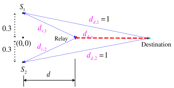
Figure 6: A symmetric two-user MARC geometry.

Towards illustrating the sum-capacity result, we consider a two-user geometry shown in Fig. 6. For this geometry, in Fig. 7 we plot the inner (DF) and outer cutset bounds on the sum-rate for $\theta=1/2$ as a function of the relay position along the x-axis. As a result of the symmetric geometry, for every choice of the relay position, both the inner and outer bounds on the sum-rate are maximized by one of cases $3a$, $3b$, or $3c$. For each case, we use an iterative algorithm, as described in the Appendix, to compute the sum-rate maximizing user policies. For cases $3a$ and $3b,$ the iterative algorithm simplifies to the iterative waterfilling algorithm developed in [37] in which at each step the algorithm finds the single-user waterfilling policy for each user while regarding the signals from the other user as noise. For case $3c$, the optimal policy at each step is still obtained by regarding the signals from the other user as noise; however, the user policy at each step is no longer a waterfilling solution. Finally, the optimality of DF when the sources are clustered relatively closer to the relay than to the destination is amply demonstrated in Fig . 7. The inner and outer bounds are also compared with the sum-capacity of the fading multiaccess channel without a relay and $\theta=1$, shown by the dashed line that is a constant independent of the relay position. Also shown in Fig 7 are the ranges of relay positions for cases $3a$, $3b,$ and $3c$ for both DF and the cutset bounds.

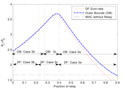
Figure 7: Plot of inner and outer bounds on the sum-rate vs. the relay position

VIII Concluding Remarks

We have developed the maximum DF sum-rate and the sum-rate optimal power policies for an ergodic fading $K$-user half-duplex Gaussian MARC. The MARC is an example of a multi-terminal network for which the multi-dimensionality of the policy set, the signal space, and the network topology space contribute to the complexity of developing capacity results resulting in few, if any, design rules for real-world communication networks. For a DF relay, the polymatroid intersection lemma allowed us to simplify the otherwise complicated analysis of developing the DF sum-rate optimal power policies for the two-user and $K$-user orthogonal MARC and the $K$-user outer bounds. The lemma allowed us to develop a broad topological classification of fading MARCs into one of following three types:

i) partially clustered MARCs where a subset of all users form a cluster with the relay while the complementary subset of users form a cluster with the destination

ii) clustered MARCs comprised of either sources-relay or relay-destination clustered networks, and

iii) arbitrarily-clustered MARCs that are a combination of either the two clustered models or of a clustered and a partially clustered model.

The optimal policies for the inner DF and the outer cutset bounds for the orthogonal half-duplex MARC model studied here lead to the following observations:

• that DF achieves the sum-capacity of a class of source-relay clustered orthogonal MARCs for which the combined link from all sources and the relay to the destination, i.e., the link achieving the $K$-user sum-rate at the destination, is the bottle-neck link. Furthermore, DF achieves the capacity region when for every weighted sum of user rates, the limiting bound is the weighted rate-sum achieved at the destination.

• that for this sum-capacity achieving case, the optimal user policies for both the orthogonal and non-orthogonal half-duplex MARCs are multi-user opportunistic waterfilling solutions over their links to the destination and the optimal relay policy is a water-filling solution over its direct link to the destination.

• and that for the remaining classes of MARCs, the optimal users policies are waterfilling and non-waterfilling solutions for the partially clustered and arbitrarily clustered models, respectively.

For the partially clustered cases, we have showed that the optimal policy for each user is multiuser waterfilling over its bottle-neck link to one of the receivers. Thus, the users that are clustered with the destination are forced to transmit at a lower rate to allow decoding of their signals at the relatively distant relay. Our results suggest that a useful practical strategy for the partially clustered topologies may be to allow those distant users that present little interference at the relay to communicate directly with the destination.

The optimal relaying strategy for all except the capacity achieving clustered case described above remains open. Given the complexity of finding the optimal signaling schemes for a given performance metric in multi-terminal networks, a natural extension to this work could be to understand the gap in spectral efficiency between DF and the cutset outer bounds for fading MARCs. Such bounds have been developed recently for time-invariant interference channels and relay channels in [38] and [39], respectively, and for fading Gaussian broadcast channels with no channel state information at the transmitter in [40].

Our analysis can also be extended to study the more general orthogonal half-duplex MARC model where the sources transmit on both orthogonal channels while the half-duplex relay is limited to receiving on one and transmitting on the other. The half-duplex relay receives signals from the sources on one of the bands while the destination receives it in both bands. For the special case where the destination can only receive in the band used by the relay to transmit, we obtain a multiple-access version of the orthogonal relay channel studied in [12]. Irrespective of the receiving capabilities of the destination, for this more general orthogonal model, each source transmits two signals, one for each band, subject to an average power constraint over both bands.

Thus, for this general model, as in [12], one can consider a more general decoding scheme of partial decode-and-forward (PDF) where each source transmits two independent messages, one on each orthogonal channel (see also [10]). As a result, the analysis does not simplify to studying an intersection of two polymatroids as it does for DF. However, analogous to the time-invariant (non-fading) case, we expect that PDF will simplify to the sum-capacity optimal DF for the special case in which all the sources and the relay are clustered. While this general orthogonal model is useful to study for the sake of completeness, the model we study here abstracts practical multi-hopping architectures and provides insights into network architectures and topologies where using a decode-and-forward relay is beneficial.

Finally, a note on complexity: our theoretic analysis distinguishes between all possible polymatroid intersection cases in determining the optimal policy for a $K$-user system and therefore has a complexity that grows exponentially in the number of users. In practice, however, for two intersecting polymatroids the maximum of a weighted sum of rates and the optimizing policies can be computed using strongly polynomial-time algorithms [26, Theorem 47.4].

[Proof of Theorem 3]

Appendix A Proof of Theorem 3

The sum-rate maximizing DF power policy $\underline{P}^{\ast}\left(\underline{H}\right)$ in Theorem 3 is obtained by sequentially determining the power policies $\underline{P}^{\left(i\right)}\left(\underline{H}\right)$ and $\underline{P}^{\left(l,n\right)}\left(\underline{H}\right)$ that maximize the sum-rate for cases $i$ and $\left(l,n\right)$, respectively, over all $\underline{P}\left(\underline{H}\right)\in\mathcal{P}$, until one of them satisfies the conditions for its case. We consider each case separately starting with case $1$.

Case 1

This case occurs when the power policy $\underline{P}\left(\underline{H}\right)\in\mathcal{B}_{1}$ is such that the intersection of the relay and destination rate regions belongs to the set of inactive cases (see Fig 2). The Lagrangian for this sum-rate maximization is given by

$$\mathcal{L}^{\left(1\right)}=S^{\left(1\right)}-\sum\nolimits_{k\in\mathcal{T}}\nu_{k}\mathbb{E}\left[P_{k}\left(\underline{H}\right)-\overline{P}_{k}\right]+\sum\nolimits_{k\in\mathcal{T}}\lambda_{k}P_{k}\left(\underline{H}\right)$$ (148)

where, for all $k\in\mathcal{T}$, $\nu_{k}$ are the dual variables associated with the power constraints in (8), $\lambda_{k}\geq 0$ are the dual variables associated with the positivity constraints $P_{k}\left(\underline{H}\right)\geq 0$, and

$$S^{\left(1\right)}=R_{\left\{1\right\},d}\left(\underline{P}\left(\underline{H}\right)\right)+R_{\left\{2\right\},r}\left(\underline{P}\left(\underline{H}\right)\right)\\ =\mathbb{E}\left[\theta C\left(\left|H_{d,1}\right|^{2}\left.P_{1}\left(\underline{H}\right)\right/\theta\right)+\overline{\theta}C\left(\left|H_{d,r}\right|^{2}\left.P_{r}\left(\underline{H}\right)\right/\overline{\theta}\right)\right]+\mathbb{E}\left[\theta C\left(\left|H_{r,2}\right|^{2}\left.P_{2}\left(\underline{H}\right)\right/\theta\right)\right].$$ (149)

The optimal policy $\underline{P}^{\left(1\right)}\left(\underline{H}\right)$ maximizes (148) if it belongs to the open set $\mathcal{B}_{1}$ defined by the conditions

$$\begin{array}[c]{ccc}R_{\left\{1\right\},d}\left(\underline{P}^{\left(1\right)}\left(\underline{H}\right)\right)<R_{\left\{1\right\},r}^{\min}\left(\underline{P}^{\left(1\right)}\left(\underline{H}\right)\right)&\text{and}&R_{\left\{2\right\},r}\left(\underline{P}^{\left(1\right)}\left(\underline{H}\right)\right)<R_{\left\{2\right\},d}^{\min}\left(\underline{P}^{\left(1\right)}\left(\underline{H}\right)\right)\end{array}$$ (150)

where

$$R_{1,r}^{\min}\left(\underline{P}\left(\underline{H}\right)\right) =\theta I(X_{1};Y_{r}|\underline{H})=\mathbb{E}\left[\theta C\left(\frac{\left|H_{r,1}\right|^{2}\left.P_{1}\left(\underline{H}\right)\right/\theta}{1+\left|H_{r,2}\right|^{2}\left.P_{2}\left(\underline{H}\right)\right/\theta}\right)\right]$$ (151)

$$R_{2,d}^{\min}\left(\underline{P}\left(\underline{H}\right)\right) =\theta I\left(X_{2};Y_{d}|\underline{H}\right).=\text{ }\mathbb{E}\left[\theta C\left(\frac{\left|H_{d,2}\right|^{2}\left.P_{2}\left(\underline{H}\right)\right/\theta}{1+\left|H_{d,1}\right|^{2}\left.P_{1}\left(\underline{H}\right)\right/\theta}\right)\right].$$ (152)

The KKT conditions for (148) simplify to

$$\begin{array}[c]{cc}\frac{\partial\mathcal{L}}{\partial P_{k}\left(\underline{h}\right)}=f_{k}^{\left(1\right)}-\nu_{k}\ln 2\leq 0,&\text{with equality for }P_{k}\left(\underline{h}\right)>0\text{, }k=1,2,r\end{array}$$ (153)

where

$$\begin{array}[c]{cc}f_{k}^{\left(1\right)}=\frac{\left|h_{m,k}\right|^{2}}{\left(1+\left|h_{m,k}\right|^{2}\left.P_{k}\left(\underline{h}\right)\right/\theta\right)}&(k,m)=(1,d),(2,r),\text{ }\end{array}$$ (155)

$$\begin{array}[c]{cc}f_{r}^{\left(1\right)}=\frac{\left|h_{d,r}\right|^{2}}{\left(1+\left|h_{d,r}\right|^{2}\left.P_{k}\left(\underline{h}\right)\right/\overline{\theta}\right)}.&\end{array}$$ (157)

It is straightforward to verify that these KKT conditions result in

$$\begin{array}[c]{ll}P_{k}^{\left(1\right)}\left(\underline{h}\right)=\left(\frac{\theta}{\nu_{k}\ln 2}-\frac{\theta}{\left|h_{m,k}\right|^{2}}\right)^{+}&(k,m)=(1,d),(2,r)\end{array}$$ (158)

and

$$P_{r}^{\left(1\right)}\left(\underline{h}\right)=\left(\frac{\overline{\theta}}{\nu_{r}\ln 2}-\frac{\overline{\theta}}{\left|h_{d,r}\right|^{2}}\right)^{+}.\text{ }$$ (159)

Case 2

With $\nu_{k}$ and $\lambda_{k}$ as the dual variables associated with the power and positivity constraints on $P_{k}$, respectively, the Lagrangian for this case is

$$\mathcal{L}^{\left(2\right)}=S^{\left(2\right)}-\sum\nolimits_{k\in\mathcal{T}}\nu_{k}\mathbb{E}\left[P_{k}\left(\underline{H}\right)-\overline{P}_{k}\right]+\sum\nolimits_{k\in\mathcal{T}}\lambda_{k}P_{k}\left(\underline{H}\right)$$ (160)

where

$$S^{\left(2\right)} =R_{\left\{1\right\},r}\left(\underline{P}\left(\underline{H}\right)\right)+R_{\left\{2\right\},d}\left(\underline{P}\left(\underline{H}\right)\right)$$ (161)

$$=\mathbb{E}\left[\theta C\left(\left|H_{r,1}\right|^{2}\left.P_{1}\left(\underline{H}\right)\right/\theta\right)+\theta C\left(\left|H_{d,2}\right|^{2}\left.P_{2}\left(\underline{H}\right)\right/\theta\right)+\overline{\theta}C\left(\left|H_{d,r}\right|^{2}\left.P_{r}\left(\underline{H}\right)\right/\overline{\theta}\right)\right].$$ (162)

The optimal policy $\underline{P}^{\left(2\right)}\left(\underline{H}\right)$ maximizes (148) if it belongs to the open set $\mathcal{B}_{2}$ given by the conditions

$$\begin{array}[c]{ccc}R_{\left\{1\right\},r}\left(\underline{P}\left(\underline{H}\right)\right)<R_{\left\{1\right\},d}^{\min}\left(\underline{P}\left(\underline{H}\right)\right)&\text{and}&R_{\left\{2\right\},d}\left(\underline{P}\left(\underline{H}\right)\right)<R_{\left\{2\right\},r}^{\min}\left(\underline{P}\left(\underline{H}\right)\right)\end{array}$$ (163)

where $R_{\left\{2\right\},r}^{\min}$ and $R_{\left\{1\right\},d}^{\min}$ are given by (151) and (152), respectively, after replacing the user indices $1$ by $2$ and 2 by 1. Note that $S^{\left(2\right)}$ and $\mathcal{L}^{\left(2\right)}$ can be obtained from $S^{\left(1\right)}$ and $\mathcal{L}^{\left(1\right)}$, respectively, by interchanging the user indices. Thus, the optimal $P_{k}^{(2)}\left(\underline{H}\right)$ and $P_{r}^{(2)}\left(\underline{H}\right)$ are given by (158) and (159), respectively, with $(k,m)=(1,r),(2,d)$ provided $P$${}^{\left(2\right)}\left(\underline{H}\right)$ satisfies (163).

Case 3

Consider the three cases $3a,$ $3b,$ and $3c$ shown in Fig. 3. The sum-rate optimization for all three cases is given by

$$\max_{\underline{P}}\min\left(R_{\mathcal{K},r},R_{\mathcal{K},d}\right)$$ (164)

subject to average power and positivity constraints on $P_{k}$ for all $k$. Recall that we write $R_{\mathcal{K},j}$ to denote the sum-rate bound at receiver $j$ where the two bounds at the relay and destination are given by (21) and (22), respectively. We write $\mathcal{B}_{3}$ to denote the open set consisting of all $\underline{P}\left(\underline{H}\right)\in\mathcal{P}$ that do not satisfy (150) and (163) either as strict inequalities, i.e., do not satisfy the conditions for cases $1$ and $2$, or as a mixture of equalities and inequalities, where by a mixture we mean that a subset of the inequalities in (150) and (163) are satisfied with equality. We will later show that such sets of mixed equalities and inequalities in (150) and (163) corresponds to conditions for the various boundary cases (see also Figs. 4 and 5). Thus, $\underline{P}\left(\underline{H}\right)\in\mathcal{B}_{3}$ only when it does not satisfy the conditions for the inactive and the active-inactive boundary cases. By definition, $\mathcal{B}_{3}$ $=$ $\mathcal{B}_{3a}\cup\mathcal{B}_{3b}\cup\mathcal{B}_{3c}$, where $\mathcal{B}_{i}$, $i=3a,3b,3c,$ is defined for case $i$ below.
The optimization in (164) is a multiuser generalization of the single-user max-min problem studied in [6] (see also [22, Sec. 3.1]) for the orthogonal single-user relay channel. In [6], the authors use a technique similar to the minimax detection rule in the two hypothesis testing problem (see for e.g., [41, II.C]) to show that the max-min problem simplifies to optimizing three disjoint cases in which the maximum rate is achieved either at the relay or at the destination or at both (boundary case). The classical results on minimax optimization also applies to the multi-user sum-rate optimization in (164), and thus, the optimal policy $\underline{P}^{\left(i\right)}\left(\underline{H}\right)$, $i=3a,3b,3c$, satisfies one of following three conditions

$$\begin{array}[c]{cc}\text{{Case 3a}:}&R_{\mathcal{K},r}|_{\underline{P}^{\left(3a\right)}\left(\underline{H}\right)}<R_{\mathcal{K},d}|_{\underline{P}^{\left(3a\right)}\left(\underline{H}\right)}\end{array}$$ (166)

$$\begin{array}[c]{cc}\text{{Case 3b}:}&R_{\mathcal{K},r}|_{\underline{P}^{\left(3b\right)}\left(\underline{H}\right)}>R_{\mathcal{K},d}|_{\underline{P}^{\left(3b\right)}\left(\underline{H}\right)}\end{array}$$ (168)

$$\begin{array}[c]{cc}\text{{Case 3c}:}&R_{\mathcal{K},r}|_{\underline{P}^{\left(3c\right)}\left(\underline{H}\right)}=R_{\mathcal{K},d}|_{\underline{P}^{\left(3c\right)}\left(\underline{H}\right)}.\end{array}$$ (170)

Note that the conditions in (166)-(170), evaluated at any $P\in\mathcal{B}_{3}$, are also conditions defining the sets $\mathcal{B}_{3a},$ $\mathcal{B}_{3b},$ and $\mathcal{B}_{3c}$, respectively. Before detailing the optimal solution for each of the above three cases, we write the Lagrangian $\mathcal{L}^{\left(i\right)}$ for case $i$ as

$$\begin{array}[c]{cc}\mathcal{L}^{\left(i\right)}=S^{\left(i\right)}-\sum\limits_{k\in\mathcal{T}}\nu_{k}\mathbb{E}\left[P_{k}\left(\underline{H}\right)-\overline{P}_{k}\right]+\sum\limits_{k\in\mathcal{T}}\lambda_{k}P_{k}\left(\underline{H}\right)&i=3a,3b,3c\end{array}$$ (172)

$$\begin{array}[c]{cc}&\text{ \ \ \ \ \ }\lambda_{k}P_{k}\left(\underline{H}\right)\geq 0\end{array}$$ (174)

where $\nu_{k}$ and $\lambda_{k}\geq 0$ are dual variables associated with the average power and positivity constraints on $P_{k}$, respectively,

$$S^{\left(i\right)}=\left\{\begin{array}[c]{ll}R_{\mathcal{K},r}=\mathbb{E}\left[C\left(\sum\limits_{k=1}^{2}\left|H_{r,k}\right|^{2}\left.P_{k}\left(\underline{H}\right)\right/\theta\right)\right]&i=3a\\ R_{\mathcal{K},d}=\mathbb{E}\left[C\left(\sum\limits_{k=1}^{2}\left|H_{d,k}\right|^{2}\left.P_{k}\left(\underline{H}\right)\right/\theta\right)\right]&i=3b\\ \left(1-\alpha\right)R_{\mathcal{K},r}+\alpha R_{\mathcal{K},d}&i=3c,\end{array}\right.$$ (175)

and $\alpha$ is the dual variable associated with the equality (boundary) condition in (170). The resulting KKT conditions are given by

$$\begin{array}[c]{cc}\frac{\partial\mathcal{L}}{\partial P_{k}\left(\underline{h}\right)}=F_{k}^{\left(i\right)}=f_{k}^{\left(i\right)}-\nu_{k}\ln 2\leq 0,&k=1,2,r,i=3a,3b,3c\end{array}$$ (176)

where (176) holds with equality for $P_{k}\left(\underline{H}\right)>0$ and for $k=1,2,$

$$f_{k}^{\left(i\right)}=\left\{\begin{array}[c]{ll}\left|h_{r,k}\right|^{2}\left/\left(1+\sum\limits_{k=1}^{2}\left|h_{r,k}\right|^{2}\left.P_{k}\left(\underline{h}\right)\right/\theta\right)\right.&i=3a\\ \left|h_{d,k}\right|^{2}\left/\left(1+\sum\limits_{k=1}^{2}\left|h_{d,k}\right|^{2}\left.P_{k}\left(\underline{h}\right)\right/\theta\right)\right.&i=3b\\ \left(1-\alpha\right)f_{k}^{\left(3a\right)}+\alpha f_{k}^{\left(3b\right)}&i=3c.\end{array}\right.$$ (177)

and $f_{r}^{\left(3a\right)}=f_{r}^{\left(3b\right)}=f_{r}^{\left(1\right)}$, $f_{r}^{\left(3c\right)}=\alpha f_{r}^{\left(1\right)}$. We now present the optimal policies and sum-rates for each case in detail.
Case 3a: For this case, the KKT conditions in (176) and (177) depend only the sum-rate and channels gains of the two users at the relay. Thus, the problem simplifies to that for a MAC channel at the relay and the classic multiuser waterfilling solution developed in [27, 28] applies. From (176), the optimal user policies are

$$\begin{array}[c]{ll}\frac{\left|h_{r,1}\right|^{2}}{v_{1}}>\frac{\left|h_{r,2}\right|^{2}}{\nu_{2}}&P_{1}^{\left(3a\right)}\left(\underline{h}\right)=\left(\frac{\theta}{\nu_{1}\ln 2}-\frac{\theta}{\left|h_{r,1}\right|^{2}}\right)^{+},P_{2}^{\left(3a\right)}=0\\ \frac{\left|h_{r,1}\right|^{2}}{v_{1}}<\frac{\left|h_{r,2}\right|^{2}}{\nu_{2}}&P_{1}^{\left(3a\right)}\left(\underline{h}\right)=0,P_{2}^{\left(3a\right)}=\left(\frac{\theta}{\nu_{2}\ln 2}-\frac{\theta}{\left|h_{r,2}\right|^{2}}\right)^{+}\\ \frac{\left|h_{r,1}\right|^{2}}{v_{1}}=\frac{\left|h_{r,2}\right|^{2}}{\nu_{2}}&\left|h_{r,1}\right|^{2}P_{1}^{\left(3a\right)}\left(\underline{h}\right)+\left|h_{r,2}\right|^{2}P_{2}^{\left(3a\right)}\left(\underline{h}\right)=\theta\left(\frac{\left|h_{r,1}\right|^{2}}{\nu_{1}\ln 2}-1\right)^{+}.\end{array}$$ (178)

With the exception of the equality condition in (178), the optimal policies are unique, i.e., the optimal $P_{k}^{\left(3a\right)}\left(\underline{H}\right)$ at user $k$ in (178) is an opportunistic water-filling solution that exploits the fading diversity in a multiaccess channel from the sources to the relay. If the channel gains are jointly distributed with a continuous density, the equality condition occurs with probability 0. Furthermore, even if the distributions were not continuous, one can choose to schedule one user or the other when the equality condition is met, thereby maintaining the opportunistic allocation policy. Finally, the optimal power policy at the relay is not explicitly obtained from $\mathcal{L}^{\left(1\right)}$ in (172) as for this case $S^{\left(1\right)}$ is the sum-rate achieved by the sources at the relay. However, since the sum-rate at the relay for this case is smaller than that at the destination, choosing the optimal waterfilling policy at the relay that maximizes the relay-destination link preserves the condition for this case, and thus, $P_{r}^{(3a)}\left(\underline{H}\right)$ is given by (159). When $P^{\left(3a\right)}\left(\underline{H}\right)\in\mathcal{B}_{3}$, the requirement of satisfying (166), i.e., $P$${}^{\left(3a\right)}\left(\underline{H}\right)$ $\in$ $\mathcal{B}_{3a}$, simplifies to a threshold condition $\overline{P}_{r}$ $>$ $P_{u}\left(\overline{P}_{1},\overline{P}_{2}\right)$ where $\overline{P}_{k}$, $k\in\mathcal{T}$, is defined in (8) and the threshold $P_{u}\left(\overline{P}_{1},\overline{P}_{2}\right)$ is obtained by setting (166) to an equality. When $P$${}^{\left(3a\right)}\left(\underline{H}\right)$ $\in$ $\mathcal{B}_{3}$ but $P$${}^{\left(3a\right)}\left(\underline{H}\right)$ $\not\in$ $\mathcal{B}_{3a}$, $R_{1}+R_{2}$ is maximized by either case 3b or case 3c. For $\underline{P}^{\left(3a\right)}\left(\underline{H}\right)$ $\not\in$ $\mathcal{B}_{3}$, as argued in Section IV, the sum-rate is not maximized by any $\underline{P}\left(\underline{H}\right)$ $\in$ $\mathcal{B}_{3}$.
Case 3b : The optimal policy $P_{k}^{\left(3b\right)}\left(\underline{H}\right)$ at user $k$ for this case satisfies the KKT conditions in (176) with $f_{k}^{\left(i\right)}=f_{k}^{\left(3b\right)}$ in (177). As with case $3a$, here too, the optimal policy is an opportunistic water-filling solution and is given by (178) with the subscript ‘$r$’ changed to ‘$d$’ for all $k$ and with the superscript $i=3b$. Further, for the relay node, the optimal $P_{r}^{\left(3b\right)}\left(H\right)$ satisfies the KKT conditions in (153), i.e., $f_{r}^{\left(3b\right)}=f_{r}^{\left(1\right)}$, and is given by the water-filling solution in (159). Finally, for $P$${}^{\left(3b\right)}\left(\underline{H}\right)$ $\in$ $\mathcal{B}_{3}$, the requirement $P$${}^{\left(3b\right)}\left(\underline{H}\right)$ $\in$ $\mathcal{B}_{3b}$ simplifies to satisfying the threshold condition $\overline{P}_{r}$ $<$ $P_{l}\left(\overline{P}_{1},\overline{P}_{2}\right)$ where $P_{l}\left(\overline{P}_{1},\overline{P}_{2}\right)$ is determined by setting (168) to an equality.
Case 3c (equal-rate policy): The optimal policy $P_{k}^{\left(3c\right)}\left(\underline{H}\right)$ at user $k$ for this case satisfies the KKT conditions in (176) for $f_{k}^{\left(i\right)}=f_{k}^{\left(3c\right)}$ in (177). The function $f_{k}^{\left(3c\right)}$ in (177) is a weighted sum of $f_{k}^{\left(3a\right)}$ and $f_{k}^{\left(3b\right)}$ where the Lagrange multiplier $\alpha$ accounts for the boundary condition in (170). Substituting $f_{k}^{(3c)}$ in (177) in (176), we have the following KKT conditions

$$\begin{array}[c]{cc}\frac{\alpha\left|h_{r,k}\right|^{2}}{1+\sum\limits_{k=1}^{2}\left|h_{r,k}\right|^{2}\frac{P_{k}\left(\underline{h}\right)}{\theta}}+\frac{\left(1-\alpha\right)\left|h_{d,k}\right|^{2}}{1+\sum\limits_{k=1}^{2}\left|h_{d,k}\right|^{2}\frac{P_{k}\left(\underline{h}\right)}{\theta}}\leq\nu_{k}\ln 2&\text{with equality for }P_{k}\left(\underline{h}\right)>0\text{, }k=1,2\end{array}$$ (179)

which implies

$$\begin{array}[c]{ll}f_{1}^{\left(3c\right)}/\nu_{1}>f_{2}^{\left(3c\right)}/\nu_{2}&P_{1}^{\left(3c\right)}\left(\underline{h}\right)=\left(\text{root of }F_{1}^{\left(3c\right)}|_{P_{2}=0}\right)^{+},P_{2}^{\left(3c\right)}\left(\underline{h}\right)=0\\ f_{1}^{\left(3c\right)}/\nu_{1}<f_{2}^{\left(3c\right)}/\nu_{2}&P_{1}^{\left(3c\right)}\left(\underline{h}\right)=0,P_{2}^{\left(3c\right)}\left(\underline{h}\right)=\left(\text{root of }F_{2}^{\left(3c\right)}|_{P_{1}=0}\right)^{+}\\ f_{1}^{\left(3c\right)}/\nu_{1}=f_{2}^{\left(3c\right)}/\nu_{2}&P_{1}^{\left(3c\right)}\left(\underline{h}\right)\text{ and }P_{2}^{\left(3c\right)}\left(\underline{h}\right)\text{ satisfy }f_{k}^{\left(3c\right)}=\nu_{k}\ln 2\end{array}$$ (180)

where $F_{k}^{\left(3c\right)}$ is defined in (176). Determining the optimal $P_{k}^{\left(3c\right)}\left(\underline{h}\right)$, $k=1,2,$ requires verifying each one of the three conditions in (180). Note that in contrast to case $3a$ (and case $3b$ with ‘$r$’ replaced in (178) by ‘$d$’), the opportunistic scheduling in (180) also depends on the user policies in addition to the channel states. Furthermore, the optimal solutions $P_{k}^{\left(3c\right)}\left(\underline{H}\right)$ do not take a water-filling form. Thus, for a given $P_{1}\left(\underline{h}\right)$, $P_{2}\left(\underline{h}\right)$ is given by

$$P_{2}\left(\underline{h}\right)=\text{positive root }x\text{ of (\ref{C3c_Eqn}) if it exists, otherwise }0$$ (181)

where the root $x$ is determined by the following equation:

$$\frac{\alpha\left|h_{r,2}\right|^{2}}{1+\left|h_{r,1}\right|^{2}\frac{P_{1}\left(\underline{h}\right)}{\theta}+\left|h_{r,2}\right|^{2}\frac{x}{\theta}}+\frac{\left(1-\alpha\right)\left|h_{d,2}\right|^{2}}{1+\left|h_{d,k}\right|^{2}\frac{P_{1}\left(\underline{h}\right)}{\theta}+\left|h_{d,k}\right|^{2}\frac{x}{\theta}}=\nu_{2}\ln 2.$$ (182)

Using $P_{2}\left(\underline{h}\right)$ given by (182), $P_{1}\left(\underline{h}\right)$ is obtained as the root of

$$\frac{\alpha\left|h_{r,1}\right|^{2}}{1+\left|h_{r,1}\right|^{2}\frac{P_{1}\left(\underline{h}\right)}{\theta}+\left|h_{r,2}\right|^{2}\frac{P_{2}\left(\underline{h}\right)}{\theta}}+\frac{\left(1-\alpha\right)\left|h_{d,1}\right|^{2}}{1+\left|h_{d,k}\right|^{2}\frac{P_{1}\left(\underline{h}\right)}{\theta}+\left|h_{d,k}\right|^{2}\frac{P_{2}\left(\underline{h}\right)}{\theta}}=\nu_{1}\ln 2.$$ (183)

Thus, for all $\underline{h}$, starting with an initial $P_{1}\left(\underline{h}\right)$, we iteratively obtain $P_{1}\left(\underline{h}\right)$ and $P_{2}\left(\underline{h}\right)$ until they converge to $P_{1}^{\left(3c\right)}\left(\underline{H}\right)$ and $P_{2}^{\left(3c\right)}\left(\underline{H}\right)$. The proof of convergence is detailed below. Finally, the optimal policies are determined over all $\alpha\in[0,1]$ to find an $\alpha^{\ast}$ that satisfies the equal rate condition in (170).

Proof of Convergence: The proof follows along the same lines as that detailed in [22, p. 3440] and relies on the fact that the maximizing function $S^{\left(3c\right)}$ in (175) is a strictly concave function of $P_{1}\left(\underline{H}\right)$ and $P_{2}\left(\underline{H}\right)$ and is bounded from above because of the power constraints at the source and relay nodes. In each iteration, the optimal $P_{1}\left(\underline{H}\right)$ and $P_{2}\left(\underline{H}\right)$ are the KKT solutions that maximize the objective function. Thus, after each iteration, the objective function either increases or remains the same. It is easy to check that for a given $P_{1}\left(\underline{H}\right)$ the objective function is a strictly concave function of $P_{2}\left(\underline{H}\right)$, and thus, (182) yields a unique value of $P_{2}\left(\underline{H}\right)$. Furthermore, the objective function is also a strictly concave function of $P_{1}\left(\underline{H}\right)$ for a fixed $P_{2}\left(\underline{H}\right)$. Thus, as the objective function converges, $\left(P_{1}\left(\underline{H}\right),P_{2}\left(\underline{H}\right)\right)$ also converge. Finally, $P_{1}\left(\underline{H}\right)$ and $P_{2}\left(\underline{H}\right)$ converge to the solutions of the KKT conditions, which is sufficient for $\left(P_{1}\left(\underline{H}\right),P_{2}\left(\underline{H}\right)\right)$ to be optimal since the objective function is concave over all $P$$\left(\underline{H}\right)\in\mathcal{P}$.

Finally, since $f_{r}^{\left(3c\right)}=\alpha f_{r}^{\left(1\right)}$, the relay’s optimal policy simplifies to the water-filling solution given by

$$\text{ }P_{r}^{\left(3c\right)}\left(\underline{H}\right)=\left(\frac{\alpha\overline{\theta}}{\nu_{r}\ln 2}-\frac{\overline{\theta}}{\left|h_{d,r}\right|^{2}}\right)^{+}.\text{ }$$ (184)

Case 4

(Boundary Cases): Recall that we define the sets $B_{i}$, $i=1,2,3a,3b,3c$, as open sets to ensure that an optimal $P$^∗ maximizes the sum-rate for a case only if it satisfies the conditions for that case. Since an optimal policy can lie on the boundary of any two such cases, we also consider six additional cases that lie at the boundary of an inactive and an active case. These boundary cases result when the conditions for an inactive case $l$, $l=1,2$, and an active case $n$, $n=3a,3b,3c$, are such that the sum-rate is the same for both cases. We consider each of the six boundary cases separately and develop the optimal $P$${}^{\left(l,n\right)}\left(\underline{H}\right)$ for each case. The requirement that the optimal $P$${}^{\left(l,n\right)}\left(\underline{H}\right)$ satisfies the condition $S^{\left(l\right)}=S^{\left(n\right)}$ for the boundary case $\left(l,n\right)$ simplifies to

$$\begin{array}[c]{ll}\text{case }\left(1,3a\right)&R_{\left\{1\right\},d}+R_{\left\{2\right\},r}=R_{\mathcal{K},r}<R_{\mathcal{K},d}\end{array}$$ (186)

$$\begin{array}[c]{ll}\text{case }\left(1,3b\right)&R_{\left\{1\right\},d}+R_{\left\{2\right\},r}=R_{\mathcal{K},d}<R_{\mathcal{K},r}\end{array}$$ (188)

$$\begin{array}[c]{ll}\text{case }\left(1,3c\right)&R_{\left\{1\right\},d}+R_{\left\{2\right\},r}=R_{\mathcal{K},r}=R_{\mathcal{K},d}\end{array}$$ (190)

$$\begin{array}[c]{ll}\text{case }\left(2,3a\right)&R_{\left\{1\right\},r}+R_{\left\{2\right\},d}=R_{\mathcal{K},r}<R_{\mathcal{K},d}\end{array}$$ (192)

$$\begin{array}[c]{ll}\text{case }\left(2,3b\right)&R_{\left\{1\right\},r}+R_{\left\{2\right\},d}=R_{\mathcal{K},d}<R_{\mathcal{K},r}\end{array}$$ (194)

$$\begin{array}[c]{ll}\text{case }\left(2,3c\right)&R_{\left\{1\right\},r}+R_{\left\{2\right\},d}=R_{\mathcal{K},d}=R_{\mathcal{K},r}\end{array}$$ (196)

where the conditions in (186)-(196) are evaluated at the appropriate $P$${}^{\left(l,n\right)}\left(\underline{H}\right)$. Note that the conditions in (186)-(196) also define the conditions for the sets $\mathcal{B}_{\left(1,3a\right)}$ through $\mathcal{B}_{\left(2,3c\right)}$, respectively. Using (186)-(196), we write the Lagrangian for all boundary cases except cases $\left(1,3c\right)$ and $\left(2,3c\right)$ as

$$\begin{array}[c]{cc}\mathcal{L}^{\left(l,n\right)}=\alpha S^{\left(l\right)}+\left(1-\alpha\right)S^{\left(n\right)}-\sum\limits_{k\in\mathcal{T}}\nu_{k}\mathbb{E}\left[P_{k}\left(\underline{H}\right)-\overline{P}_{k}\right]+\sum\limits_{k\in\mathcal{T}}\lambda_{k}P_{k}\left(\underline{H}\right)&l=1,2,n=3a,3b\end{array}$$ (198)

$$\lambda_{k}P_{k}\left(\underline{H}\right)\geq 0$$ (199)

and the Lagrangian for cases $\left(1,3c\right)$ and $\left(2,3c\right)$ as

$$\mathcal{L}^{\left(l,3c\right)}=\alpha_{1}S^{\left(l\right)}+\alpha_{2}S^{\left(3a\right)}+\left(1-\alpha_{1}-\alpha_{2}\right)S^{\left(3b\right)}-\sum\limits_{k\in\mathcal{T}}\nu_{k}\mathbb{E}\left[P_{k}\left(\underline{H}\right)-\overline{P}_{k}\right]$$

$$\begin{array}[c]{ccc}&\text{ \ \ \ \ \ }+\sum\limits_{k\in\mathcal{T}}\lambda_{k}P_{k}\left(\underline{H}\right),&l=1,2\end{array}$$ (201)

$$\lambda_{k}P_{k}\left(\underline{H}\right)\geq 0$$ (202)

where $\nu_{k}$ and $\lambda_{k}\geq 0$ are dual variables associated with the average power and positivity constraints on $P_{k}$, respectively. The variable $\alpha$ is the dual variable associated with all boundary cases with a single boundary condition while $\alpha_{1}$ and $\alpha_{2}$ are the dual variables associated with cases $\left(1,3c\right)$ and $\left(2,3c\right)$. The resulting KKT conditions, one for each $P_{k}\left(\underline{h}\right)$, $k=1,2,r,$ are

$$\begin{array}[c]{cc}\text{Case }\left(l,n\not=3c\right):&\frac{\partial\mathcal{L}^{\left(l,n\right)}}{\partial P_{k}\left(\underline{h}\right)}=f_{k}^{\left(l,n\right)}=\alpha f_{k}^{\left(l\right)}+\left(1-\alpha\right)f_{k}^{\left(n\right)}\leq\nu_{k}\ln 2\end{array}$$ (204)

$$\begin{array}[c]{cc}\text{Case }\left(l,n=3c\right):&\frac{\partial\mathcal{L}^{\left(l,n\right)}}{\partial P_{k}\left(\underline{h}\right)}=f_{k}^{\left(l,n\right)}=\alpha_{1}f_{k}^{\left(l\right)}+\alpha_{2}f_{k}^{\left(3a\right)}+\left(1-\alpha_{1}-\alpha_{2}\right)f_{k}^{\left(3b\right)}\leq\nu_{k}\ln 2\end{array}$$ (206)

where $f_{k}^{\left(l\right)}$ and $f_{k}^{\left(n\right)}$ are as defined earlier for cases $l$ and $n$ and equality holds in (204) and (206) for $P_{k}\left(\underline{h}\right)>0$, for all $\underline{h}$. We now present the optimal policies for each case separately.
Case $\left(1,3a\right)$: From (204), the KKT conditions for this case are

$$\begin{array}[c]{cc}f_{1}^{\left(1,3a\right)}=\frac{\alpha\left|h_{d,1}\right|^{2}}{1+\left|h_{d,1}\right|^{2}P_{1}\left(\underline{h}\right)/\theta}+\frac{\left(1-\alpha\right)\left|h_{r,1}\right|^{2}}{1+\sum\nolimits_{j=1}^{2}\left|h_{r,j}\right|^{2}P_{j}\left(\underline{h}\right)/\theta}\leq\nu_{1}\ln 2&\text{with equality if }P_{1}\left(\underline{h}\right)>0\end{array}$$ (208)

$$\begin{array}[c]{cc}f_{2}^{\left(1,3a\right)}=\frac{\alpha\left|h_{r,2}\right|^{2}}{1+\left|h_{r,2}\right|^{2}P_{2}\left(\underline{h}\right)/\theta}+\frac{\left(1-\alpha\right)\left|h_{r,2}\right|^{2}}{1+\sum\nolimits_{j=1}^{2}\left|h_{r,j}\right|^{2}P_{j}\left(\underline{h}\right)/\theta}\leq\nu_{2}\ln 2&\text{with equality if }P_{2}\left(\underline{h}\right)>0\end{array}$$ (210)

$$\begin{array}[c]{cc}f_{r}^{\left(1,3a\right)}=\frac{\alpha\left|h_{d,r}\right|^{2}}{1+\left|h_{d,r}\right|^{2}P_{r}\left(\underline{h}\right)/\overline{\theta}}\leq\nu_{r}\ln 2&\text{with equality if }P_{r}\left(\underline{h}\right)>0\end{array}$$ (212)

which implies

$$\begin{array}[c]{ll}\frac{f_{1}^{\left(1,3a\right)}}{\nu_{1}}>\frac{f_{2}^{\left(1,3a\right)}}{\nu_{2}}&P_{1}\left(\underline{h}\right)=\left(\text{root of }F_{1}^{\left(1,3a\right)}|_{P_{2}=0}\right)^{+},P_{2}\left(\underline{h}\right)=0\\ \frac{f_{1}^{\left(1,3a\right)}}{\nu_{1}}<\frac{f_{2}^{\left(1,3a\right)}}{\nu_{2}}&P_{1}\left(\underline{h}\right)=0,P_{2}\left(\underline{h}\right)=\left(\text{root of }F_{2}^{\left(1,3a\right)}|_{P_{1}=0}\right)^{+}\\ \frac{f_{1}^{\left(1,3a\right)}}{\nu_{1}}=\frac{f_{2}^{\left(1,3a\right)}}{\nu_{2}}&P_{1}\left(\underline{h}\right)\text{ and }P_{2}\left(\underline{h}\right)\text{ satisfy }\frac{f_{1}^{\left(1,3a\right)}}{\nu_{1}}=\frac{f_{2}^{\left(1,3a\right)}}{\nu_{2}}\end{array}$$ (213)

where

$$\begin{array}[c]{cc}F_{k}^{\left(l,n\right)}=f_{k}^{\left(l,n\right)}-\nu_{k}\ln 2\leq 0,&\text{for all }\left(l,n\right).\end{array}$$ (214)

As in case $3c$, the optimal policies take an opportunistic non-waterfilling form and in fact can be obtained by the iterative algorithm described for that case. Finally, from (212), the optimal $P_{r}^{\left(1,3a\right)}\left(\underline{H}\right)$ is given by (184).
Case $\left(1,3b\right)$: The analysis for this case mirrors that for case $\left(1,3a\right)$ and the optimal user policies are opportunistic non-water-filling solution given by (213) with $f_{k}^{\left(3a\right)}$ replaced by $f_{k}^{\left(3b\right)}$, $k=1,2$. On the other hand in contrast to case $\left(1,3a\right)$ where $f_{r}^{\left(3a\right)}=0$, since both $f_{r}^{\left(1\right)}$ and $f_{r}^{\left(3b\right)}$ are non-zero, the optimal relay policy $P_{r}^{\left(2,3a\right)}=$ $P_{r}^{\left(1\right)}$.
Case $\left(1,3c\right)$: For this case, the KKT conditions in (206) involves a weighted sum of $f_{k}^{\left(l\right)}$, $f_{k}^{\left(3a\right)}$, and $f_{k}^{\left(3b\right)}$. Thus, for $k=1,2$, $(k,m)=(1,d),(2,r)$, we have the KKT conditions

$$\begin{array}[c]{cc}f_{1}^{\left(1,3c\right)}=\alpha_{1}f_{1}^{\left(1\right)}+\alpha_{2}f_{1}^{\left(3a\right)}+\left(1-\alpha_{1}-\alpha_{2}\right)f_{1}^{\left(3b\right)}\leq\nu_{1}\ln 2&\text{with equality if }P_{1}\left(\underline{h}\right)>0\end{array}$$ (216)

$$\begin{array}[c]{cc}f_{2}^{\left(1,3c\right)}=\alpha_{1}f_{2}^{\left(1\right)}+\alpha_{2}f_{2}^{\left(3a\right)}+\left(1-\beta\right)\left(1-\alpha\right)f_{2}^{\left(3b\right)}\leq\nu_{2}\ln 2&\text{with equality if }P_{2}\left(\underline{h}\right)>0\end{array}$$ (218)

$$\begin{array}[c]{cc}f_{r}^{\left(1,3c\right)}=\left(1-\alpha_{2}\right)\left|h_{d,r}\right|^{2}\left/C\left(\left|h_{d,r}\right|^{2}P_{r}/\overline{\theta}\right)\right.\leq\nu_{r}\ln 2&\text{with equality if }P_{r}\left(\underline{h}\right)>0\end{array}$$ (220)

where $\alpha_{1}$ and $\alpha_{2}$ are the dual variables associated with the equalities $R_{\mathcal{K},d}=R_{\left\{1\right\},d}+R_{\left\{2\right\},r}$ and $R_{\mathcal{K},d}=R_{\mathcal{K},r}$, respectively, in (190). From (216) and (218), one can verify that the optimal user policies are opportunistic non-waterfilling solutions given by (213) with the superscript $\left(1,3a\right)$ replaced by $\left(1,3c\right)$. Finally, $P_{r}^{\left(1,3c\right)}\left(\underline{H}\right)$ is given by the water-filling solution in (159) with $\alpha$ replaced by $\left(1-\alpha_{2}\right)$.
Case $\left(2,3a\right)$: The optimal user policies for this case and the KKT conditions they satisfy are given by (208), (210), and (213) when $f_{k}^{\left(1\right)}$ is replaced by $f^{\left(2\right)}$, for all $k$, and $g_{k}^{\left(\cdot\right)}$ is superscripted by $\left(2,3a\right)$. Thus, here too, the optimal user policies are opportunistic non-water-filling solutions. The optimal relay policy $P_{r}^{\left(2,3a\right)}\left(\underline{H}\right)$ is the same as that obtained in case $\left(1,3a\right)$.
Case $\left(2,3b\right)$: The optimal user policies $P_{k}^{\left(2,3b\right)}\left(\underline{H}\right)$, $k=1,2,$ are again opportunistic non-water-filling solutions and are given by (208), (210), and (213) when $f_{k}^{\left(1\right)}$ and $f_{k}^{\left(3a\right)}$ are replaced by $f^{\left(2\right)}$ and $f^{\left(3b\right)}$, respectively, for all $k$, and $g_{k}^{\left(\cdot\right)}$ is superscripted by $\left(2,3b\right)$. The optimal relay policy $P_{r}^{\left(2,3b\right)}\left(\underline{H}\right)$ is the same as that for case $\left(1,3b\right)$.
Case $\left(2,3c\right)$: The optimal policy vector $P$${}^{(2,3c)}\left(\underline{H}\right)$ is the same as that for case $\left(1,3c\right)$ with $f_{k}^{\left(1\right)}$ is replaced by $f^{\left(2\right)}$, for all $k$, and with the superscript $\left(2,3c\right)$.

References

- [1] A. Sendonaris, E. Erkip, and B. Aazhang, “User cooperation diversity - part I: System description,” IEEE Trans. Commun., vol. 51, no. 11, pp. 1927–1938, Nov. 2003.
- [2] J. N. Laneman, D. N. C. Tse, and G. Wornell, “Cooperative diversity in wireless networks: Efficient protocols and outage behavior,” IEEE Trans. Inform. Theory, vol. 50, no. 12, pp. 3062–3080, Dec. 2004.
- [3] G. Kramer, M. Gastpar, and P. Gupta, “Cooperative strategies and capacity theorems for relay networks,” IEEE Trans. Inform. Theory, vol. 51, no. 9, pp. 3027–3063, Sept. 2005.
- [4] K. Azarian, H. El Gamal, and P. Schniter, “On the achievable diversity-multiplexing tradeoff in half-duplex cooperative channels,” IEEE Trans. Inform. Theory, vol. 51, no. 12, pp. 4152–4172, Dec. 2005.
- [5] A. Host-Madsen and J. Zhang, “Capacity bounds and power allocation for the wireless relay channel,” IEEE Trans. Inform. Theory, vol. 51, no. 6, pp. 2020–2040, June 2005.
- [6] Y. Liang and V. Veeravalli, “Resource allocation for wireless relay channels,” in Proc. 38th Annual Asilomar Conf. Signals, Systems, and Computers, Pacific Grove, CA, Nov. 2004.
- [7] L. Sankaranarayanan, G. Kramer, and N. B. Mandayam, “Cooperative diversity in wireless networks: A geometry-inclusive analysis,” in Proc. 43rd Annual Allerton Conf. on Commun., Control, and Computing, Monticello, IL, Sept. 2005.
- [8] G. Kramer and A. J. van Wijngaarden, “On the white Gaussian multiple-access relay channel,” in Proc. 2000 IEEE Int. Symp. Inform. Theory, Sorrento, Italy, June 2000, p. 40.
- [9] T. Cover and A. El Gamal, “Capacity theorems for the relay channel,” IEEE Trans. Inform. Theory, vol. 25, no. 5, pp. 572–584, Sept. 1979.
- [10] L. Sankaranarayanan, G. Kramer, and N. B. Mandayam, “Hierarchical sensor networks: Capacity theorems and cooperative strategies using the multiple-access relay channel model,” in Proc. First IEEE Conference on Sensor and Ad Hoc Communications and Networks, Santa Clara, CA, Oct. 2004.
- [11] L. Sankar, G. Kramer, and N. B. Mandayam, “Offset encoding for multiaccess relay channels,” IEEE Trans. Inform. Theory, vol. 53, no. 10, pp. 1–8, Oct. 2007.
- [12] A. El Gamal and S. Zahedi, “Capacity of relay channels with orthogonal components,” IEEE Trans. Inform. Theory, vol. 51, no. 5, pp. 1815–1817, May 2005.
- [13] M. Yuksel and E. Erkip, “Multi-antenna cooperative wireless systems: A diversity-multiplexing tradeoff perspective,” IEEE Trans. Inform. Theory, vol. 53, no. 10, pp. 3371–3393, Oct. 2007.
- [14] D. Gunduz and E. Erkip, “Opportunistic cooperation by dynamic resource alloation,” IEEE Trans. Wireless Commun., vol. 6, no. 4, pp. 1446–1454, Apr. 2007.
- [15] A. S. Avestimehr and D. N. C. Tse, “Outage capacity of the fading relay channel in the low SNR regime,” IEEE Trans. Inform. Theory, vol. 53, no. 4, pp. 1401–1415, Apr. 2007.
- [16] L. Sankar, G. Kramer, and N. B. Mandayam, “User vs. relay cooperation in time-duplexed multi-access relay networks,” Aug. 2008, arxiv.org e-print 0809.2226.
- [17] R. Liu, J. Luo, and P. Spasojevic, “Adaptive transmission with variable-rate turbo bit-interleaved coded modulation,” IEEE Trans. Wireless Commun., vol. 6, no. 11, pp. 3926–2936, Nov. 2007.
- [18] A. Stefanov and E. Erkip, “Cooperative coding for wireless networks,” IEEE Trans. Commun., vol. 52, no. 8, pp. 3926–2936, Sept. 2004.
- [19] I. Maric and R. Yates, “Forwarding strategies for Gaussian parallel-relay networks,” in Proc. 2004 IEEE Int. Symp. Inform. Theory, Chicago, IL, June 2004.
- [20] ——, “Bandwidth and power allocation for cooperative strategies in Gaussian relay networks,” in Proc. 38th Annual Asilomar Conf. Signals, Systems, and Computers, Pacific Grove, CA, Nov. 2004.
- [21] Y. Yao, X. Cai, and G. B. Giannakis, “On energy efficiency and optimum resource allocation of relay transmissions in the low-power regime,” IEEE Trans. Wireless Commun., vol. 4, no. 6, pp. 2917–2927, Nov. 2005.
- [22] Y. Liang, V. Veeravalli, and H. V. Poor, “Resource allocation for wireless fading relay channels: Max-min solution,” IEEE Trans. Inform. Theory, vol. 53, no. 10, pp. 3432–3453, Oct. 2007.
- [23] W. Mesbah and T. N. Davidson, “Power and resource allocation for orthogonal multiple access relay systems,” in Proc. 2008 IEEE Intl. Symp. Inform. Theory, Toronto, Canada, July 2008.
- [24] O. Oyman, “Opportunism in multiuser relay channels: Scheduling, routing, and spectrum reuse,” in Proc. 2007 IEEE Intl. Symp. Inform. Theory, Nice, France, June 2007.
- [25] S. Serbetli and A. Yener, “Relay assisted f/tdms ad hoc networks: Node classification, power allocation, and relaying strategies,” IEEE Trans. Commun., vol. 56, no. 6, pp. 937–947, June 2008.
- [26] A. Schrijver, Combinatorial Optimization: Polyhedra and Efficiency. New York: Springer-Verlag, 2003.
- [27] R. Knopp and P. Humblet, “Information capacity and power control in single-cell multiuser communications,” in Proc. IEEE Intl. Conf. Commun., Seattle, WA, June 1995.
- [28] D. N. C. Tse and S. V. Hanly, “Multiaccess fading channels - part I: Polymatroid structure, optimal resource allocation and throughput capacities,” IEEE Trans. Inform. Theory, vol. 44, no. 7, pp. 2796–2815, Nov. 1998.
- [29] L. Sankar, N. B. Mandayam, and H. V. Poor, “On the sum-capacity of degraded Gaussian multiaccess relay channels,” Mar. 2008, arxiv.org e-print 0804.0385.
- [30] T. S. Han, “The capacity region of general multiple-access channel with certain correlated sources,” Information and Control, vol. 40, no. 1, pp. 37–60, Jan. 1979.
- [31] L. Sankar, “Relay Cooperation in Multiaccess Networks,” Ph.D. dissertation, Rutgers, The State University of New Jersey, New Brunswick, NJ, 2007. [Online]. Available: http://www.winlab.rutgers.edu/lalitha
- [32] S. Boyd and L. Vandenberghe, Convex Optimization. Cambridge, UK: Cambridge University Press, 2004.
- [33] A. Goldsmith and P. Varaiya, “Capacity of fading channels with channel side information,” IEEE Trans. Inform. Theory, vol. 43, no. 6, pp. 1986–1992, Nov. 1997.
- [34] H. G. Eggleston, Convexity. Cambridge, UK: Cambridge University Press, 1958.
- [35] G. Kramer, “Models and theory for relay channels with receive constraints,” in 42nd Annual Allerton Conf. on Commun., Control, and Computing, Monticello, IL, Sept. 2004.
- [36] W. Yu and W. Rhee, “Degrees of freedom in wireless multiuser spatial multiplex systems with multiple antennas,” IEEE Trans. Commun., vol. 54, no. 10, pp. 1747–1753, Oct. 2006.
- [37] ——, “Iterative water-filling for Gaussian vector multiple-access channels,” IEEE Trans. Inform. Th., vol. 50, no. 1, pp. 145–152, Jan. 2004.
- [38] G. Bresler and D. N. C. Tse, “The two-user gaussian interference channel: a deterministic view,” Euro. Trans. Telecomm., vol. 19, no. 4, pp. 333–354, June 2008.
- [39] S. Avestimehr, S. Diggavi, and D. N. C. Tse, “Wireless network information flow: a deterministic approach,” Oct. 2007, arxiv.org e-print 0710.3781.
- [40] D. Tse, R. Yates, and Z. Li, “Fading broadcast channels with state information at the receivers,” in Proc. 46th Annual Allerton Conf. on Commun., Control, and Computing, Monticello, IL, Sept. 2008.
- [41] H. V. Poor, An Introduction to Signal Detection and Estimation, 2nd. Ed. New York: Springer-Verlag, 1994.