Variational approach to complicated similarity solutions of higher-order nonlinear PDEs. I

Abstract.

The Cauchy problem for $(x,t)\in{\mathbb{R}}^{N}\times{\mathbb{R}}_{+}$ for three higher-order degenerate quasilinear PDEs, as basic models,

$$\begin{matrix}u_{t}=(-1)^{m+1}\Delta^{m}(|u|^{n}u)+|u|^{n}u,\qquad\,\quad\vskip 3.0pt plus 1.0pt minus 1.0pt\\ u_{tt}=(-1)^{m+1}\Delta^{m}(|u|^{n}u)+|u|^{n}u,\qquad\quad\vskip 3.0pt plus 1.0pt minus 1.0pt\\ u_{t}=(-1)^{m+1}[\Delta^{m}(|u|^{n}u)]_{x_{1}}+(|u|^{n}u)_{x_{1}},\end{matrix}$$

where $n>0$ is a fixed exponent and $\Delta^{m}$ is the $(m\geq 2)$th iteration of the Laplacian, is studied. This diverse class of degenerate PDEs embraces equations of different three types: parabolic, hyperbolic, and nonlinear dispersion. Such degenerate evolution equations from various applications in mechanics and physics admitting compactly supported and blow-up solutions attracted attention of the mathematicians since the 1970-80s.

In the present paper, some general local, global, and blow-up features of such PDEs on the basis of construction of their blow-up similarity and travelling wave solutions are revealed. Blow-up, i.e., nonexistence of global in time solutions is proved by various methods. In particular, for $m=2$ and $m=3$, such similarity patterns lead to the following semilinear fourth- and sixth-order elliptic PDEs with non-coercive operators and non-Lipschitz nonlinearities:

(0.1) $$-\Delta^{2}F+F-|F|^{-\frac{n}{n+1}}F=0\quad\mbox{and}\quad\Delta^{3}F+F-|F|^{-\frac{n}{n+1}}F=0\quad\mbox{in}\quad{\mathbb{R}}^{N}\times{\mathbb{R}}_{+},$$

which were not addressed before in the mathematical literature. The goal is, using a variety of analytic variational, qualitative, and, often, numerical methods, to justify that equations (0.1) admit an infinite at least countable set of countable families of compactly supported solutions that are oscillatory near finite interfaces. In a whole, this solution set exhibit typical features of being of a chaotic structure.

The present paper is an earlier extended version of [17]. In particular, here we pay more attention to some category/fibering aspects of critical values and points, as well as to sixth and higher-order equations with $m\geq 3$, while in [17] the case $m=2$ was under maximally detailed scrutiny.

1. Introduction: higher-order models and blow-up/compacton solutions

1.1. Three types of nonlinear PDEs under consideration

We describe common local and global properties of weak compactly solutions of classes of nonlinear partial differential equations (PDEs) of parabolic, hyperbolic, and nonlinear dispersion type:

(I) $2m$th-order quasilinear parabolic equations with regional blow-up,

(II) $2m$th-order quasilinear hyperbolic equations with regional blow-up, and

(III) ($2m$+1)th-order nonlinear dispersion equations with compactons.

Therefore, we plan to study some common local and global properties of weak compactly solutions of three classes of quasilinear partial differential equations (PDEs) of parabolic, hyperbolic, and nonlinear dispersion type, which, in general, look like having nothing in common. Studying and better understanding of nonlinear degenerate PDEs of higher-order including a new class of less developed nonlinear dispersion equations (NDEs) from compacton theory are striking features of modern general PDE theory at the beginning of the twenty first century. It is worth noting and realizing that several key theoretical demands of modern mathematics are already associated and connected with some common local and global features of nonlinear evolution PDEs of different types and orders, including higher-order parabolic, hyperbolic, nonlinear dispersion, and others as typical representatives.

Regardless the great progress of PDE theory achieved in the twentieth century for many key classes of nonlinear equations [6], the transition process to higher-order degenerate PDEs with more and more complicated non-monotone, non-potential, and non-symmetric nonlinear operators will require different new methods and mathematical approaches. Moreover, it seems that, for some types of such nonlinear higher-order problems, the entirely rigorous “exhaustive” goal of developing a complete description of solutions, their properties, functional settings of problems of interest, etc., cannot be achieved in principle, in view of an extremal variety of singular, bifurcation, and branching phenomena that are contained in such multi-dimensional evolution. In many cases, the main results should be extracted by a combination of methods of various analytic, qualitative, and numerical origins. In many cases, the main results should be extracted by a combination of methods of various analytic, qualitative, and numerical origins.

In the present paper, we deal with complicated pattern sets, where, for the elliptic problems in ${\mathbb{R}}^{N}$ and even for the corresponding one-dimensional ODE reductions, using the proposed analytic-numerical approaches is necessary and unavoidable. As a first illustration of such features, let us mention that, according to our current experience, for such classes of second-order $C^{1}$ variational problems,

$$\begin{matrix}\mbox{distinguishing the classic Lusternik--Schnirel'man countable sequence of$\quad\,\,\,\,\,\,$}\\ \mbox{critical values and points is not possible without refined numerical methods},\end{matrix}$$

in view of huge complicated multiplicity of other admitted solutions. It is essential, that the arising problems do not admit, as customary for other classes of elliptic equations, any homotopy classification of solutions (say, on the hodograph plane), since all the compactly supported solutions are infinitely oscillatory that makes the homotopy rotational parameter infinite and hence the method non-applicable.

Let us now introduce these three classes, (I)–(III), of PDEs and corresponding nonlinear phenomena to be studied by some unified approaches.

1.2. (I) Combustion models: regional blow-up, global stability, main goals, and first discussion

We begin with the following quasilinear degenerate $2m$th-order parabolic equation of reaction-diffusion (combustion) type:

(1.1) $$u_{t}=(-1)^{m+1}\Delta^{m}(|u|^{n}u)+|u|^{n}u\quad\mbox{in}\quad{\mathbb{R}}^{N}\times{\mathbb{R}}_{+},$$

where $n>0$ is a fixed exponent, $m\geq 2$ is integer, and $\Delta$ denoted the Laplace operator in ${\mathbb{R}}$.

Globally asymptotically stable exact blow-up solutions of S-regime. In the simplest case $m=1$ and $N=1$, (1.1) is nowadays the canonical quasilinear heat equation

(1.2) $$u_{t}=(u^{n+1})_{xx}+u^{n+1}\quad\mbox{in}\quad{\mathbb{R}}\times{\mathbb{R}}_{+}\quad(u\geq 0),$$

which occurs in combustion theory. The reaction-diffusion equation (1.2), playing a key role in blow-up PDE theory, was under scrutiny since the middle of the 1970s. In 1976, Kurdyumov, with his former PhD students, Mikhailov and Zmitrenko (q.v. [38] and [37, Ch. 4] for history) discovered the phenomenon of heat and combustion localization by studying the blow-up separate variables Zmitrenko–Kurdyumov solution of (1.2):

(1.3) $$u_{\rm S}(x,t)=(T-t)^{-\frac{1}{n}}f(x)\quad\mbox{in}\quad{\mathbb{R}}\times(0,T),$$

where $T>0$ is the blow-up time, and $f$ satisfies the ODE

(1.4) $$\frac{1}{n}\,f=(f^{n+1})^{\prime\prime}+f^{n+1}\quad\mbox{for}\,\,\,\,x\in{\mathbb{R}}.$$

It turned out that (1.4) possesses the explicit compactly supported solution

(1.5) $$f(x)=\left\{\begin{matrix}\bigl{[}\frac{2(n+1)}{n(n+2)}\,\cos^{2}\bigl{(}\frac{nx}{2(n+1)}\bigr{)}\bigr{]}^{\frac{1}{n}},\quad\,\mbox{if}\,\,\,\,\,\,\,|x|\leq\frac{n+1}{n}\,\pi,\cr\qquad\,\qquad 0,\qquad\qquad\,\,\,\,\,\,\,\quad\,\mbox{if}\,\,\,\,\,\,\,|x|>\frac{n+1}{n}\,\pi.\end{matrix}\right.$$

This explicit integration of the ODE (1.4) was amazing and rather surprising in the middle of the 1970s and led then to the foundation of blow-up and heat localization theory. In dimension $N>1$, the blow-up solution (1.3) does indeed exist [37, p. 183] but not in an explicit form (so that, it seems, 1.5) is the only available elegant form).

Blow-up S-regime for higher-order parabolic PDEs. Evidently, the $2m$th-order counterpart (1.1) admits the regional blow-up solution of the same form (1.3), but the profile $f=f(y)$ then solves a more complicated ODE

(1.6) $$(-1)^{m+1}\Delta^{m}(|f|^{n}f)+|f|^{n}f=\frac{1}{n}\,f\quad\mbox{in}\,\,\,{\mathbb{R}}^{N}.$$

After natural change, this gives the following equation with a non-Lipschitz nonlinearity:

$$F=|f|^{n}f\quad\Longrightarrow\quad\mbox{$(-1)^{m+1}\Delta^{m}F+F-\frac{1}{n}\,\big{|}F\big{|}^{-\frac{n}{n+1}}F=0\quad\mbox{in}\,\,\,{\mathbb{R}}^{N}.$}$$

Finally, we scale out the multiplier $\frac{1}{n}$ in the nonlinear term,

(1.7) $$F\mapsto n^{-\frac{n+1}{n}}F\quad\Longrightarrow\quad\framebox{$(-1)^{m+1}\Delta^{m}F+F-\big{|}F\big{|}^{-\frac{n}{n+1}}F=0\quad\mbox{in}\,\,\,{\mathbb{R}}^{N}.$}$$

In the one-dimensional case $N=1$, we obtain a simpler ODE,

(1.8) $$F\mapsto n^{-\frac{n+1}{n}}F\quad\Longrightarrow\quad\framebox{$(-1)^{m+1}F^{(2m)}+F-\big{|}F\big{|}^{-\frac{n}{n+1}}F=0\quad\mbox{in}\,\,\,{\mathbb{R}}.$}$$

Thus, according to (1.3), the elliptic problems (1.7) and the ODE (1.8) for $N=1$ are responsible for the possible “geometrical shapes” of regional blow-up described by the higher-order combustion model (1.1).

Plan and main goals of the paper related to parabolic PDEs. Unlike the second-order case (1.5), explicit compactly supported solutions $F(x)$ of (1.8) for any $m\geq 2$ are not available. Moreover, it turns out that such profiles $F(x)$ have rather complicated local and global structure. We are not aware of any rigorous or even formal qualitative results concerning existence, multiplicity, or global structure of solutions of ODEs such as (1.8). Our main goals are four-fold:

(ii) Problem “Blow-up”: proving finite-time blow-up in the parabolic (and hyperbolic) PDEs under consideration (Section 2);

(ii) Problem “Multiplicity”: existence and multiplicity for elliptic PDEs (1.7) and the ODEs (1.8) (Section 3);

(iii) Problem “Oscillations”: the generic structure of oscillatory solutions of (1.8) near interfaces (Section 4); and

(iv) Problem “Numerics”: numerical study of various families of $F(x)$ (Sections 5, 6).

The research will be continued in the second half of this paper [18], where we intend to refine our results on the multiplicity of solutions (especially, for $m>2$), pose the problem on a “Sturm index” of solutions (a homotopy classification of some sub-families of solutions), and introduce and study related analytic models with similar families of solutions.

Thus, in particular, we show that ODEs (1.8), as well as the PDE (1.7), for any $m\geq 2$ admit infinitely many countable families of compactly supported solutions in ${\mathbb{R}}$, and the whole solution set exhibits certain chaotic properties. Our analysis will be based on a combination of analytic (variational and others), numerical, and various formal techniques. Explaining existence, multiplicity, and asymptotics for the nonlinear problems involved, we leave several open mathematical problems. Some of these for higher-order equations are extremely difficult.

1.3. (II) Regional blow-up in quasilinear hyperbolic equations

Secondly, consider the $2m$th-order hyperbolic counterpart of (1.1),

(1.9) $$u_{tt}=(-1)^{m+1}\Delta^{m}(|u|^{n}u)+|u|^{n}u\quad\mbox{in}\quad{\mathbb{R}}^{N}\times{\mathbb{R}}_{+}.$$

We begin the discussion of its blow-up solutions in 1D, i.e., for

(1.10) $$u_{tt}=(u^{n+1})_{xx}+u^{n+1}\quad\mbox{in}\quad{\mathbb{R}}\times{\mathbb{R}}_{+}\quad(u\geq 0).$$

Here the blow-up solutions and the ODE take the form

(1.11) $$u_{\rm S}(x,t)=(T-t)^{-\frac{2}{n}}\tilde{f}(x)\quad\Longrightarrow\quad\frac{2}{n}\bigl{(}\frac{2}{n}+1\bigr{)}\,\tilde{f}=(\tilde{f}^{n+1})^{\prime\prime}+\tilde{f}^{n+1}.$$

Using extra scaling,

(1.12) $$\tilde{f}(x)=\bigl{[}\frac{2(n+2)}{n}\bigr{]}^{\frac{1}{n}}f(x)$$

yields the same ODE (1.4) and hence the exact localized solution (1.5).

For the $N$-dimensional PDE (1.9), looking for the same solution (1.11), after scaling, leads to the elliptic equation (1.7).

1.4. (III) Nonlinear dispersion equations and compactons

In a general setting, these rather unusual PDEs take the form

(1.13) $$u_{t}=(-1)^{m+1}[\Delta^{m}(|u|^{n}u)]_{x_{1}}+(|u|^{n}u)_{x_{1}}\quad\mbox{in}\quad{\mathbb{R}}^{N}\times{\mathbb{R}}_{+},$$

where the right-hand side is just the derivation $D_{x_{1}}$ of that in the parabolic counterpart (1.1). Then the elliptic problem (1.7) occurs when studying travelling wave (TW) solutions of (1.13). As usual, we explain this first in a simpler 1D case.

Let $N=1$ and $m=1$ in (1.13) that yields the third-order Rosenau–Hyman (RH) equation

(1.14) $$u_{t}=(u^{2})_{xxx}+(u^{2})_{x},$$

which is known to model the effect of nonlinear dispersion in the pattern formation in liquid drops [36]. It is the $K(2,2)$ equation from the general $K(m,n)$ family of nonlinear dispersion equations (NDEs)

(1.15) $$u_{t}=(u^{n})_{xxx}+(u^{m})_{x}\quad(u\geq 0),$$

that also describe phenomena of compact pattern formation, [33, 34]. In addition, such PDEs appear in curve motion and shortening flows [35]. Similar to the previous models, the $K(m,n)$ equation (1.15) with $n>1$ is degenerated at $u=0$, and therefore may exhibit finite speed of propagation and admit solutions with finite interfaces. A permanent source of NDEs is integrable equation theory, e.g. look at the integrable fifth-order Kawamoto equation [23] (see [20, Ch. 4] for other models), which is of NDE’s type:

(1.16) $$u_{t}=u^{5}u_{xxxxx}+5\,u^{4}u_{x}u_{xxxx}+10\,u^{5}u_{xx}u_{xxx}.$$

Questions of local existence, uniqueness, regularity, shock and rarefaction wave formation, finite propagation and interfaces, including degenerate higher-order models to be studied are treated in [19, 14]; see also comments in [20, Ch. 4.2].

We will study some particular continuous solutions of the NDEs that give insight on several generic properties of such nonlinear PDEs. The crucial advantage of the RH equation (1.14) is that it possesses explicit moving compactly supported soliton-type solutions, called compactons [36], which are travelling wave (TW) solutions:

Compactons: manifolds of TWs and blow-up S-regime solutions coincide. Let us show that such compactons are directly related to the blow-up patterns presented above. Actually, explicit TW compactons exist for the nonlinear dispersion KdV-type equations with arbitrary power nonlinearities (formulae will be given shortly)

(1.17) $$u_{t}=(u^{n+1})_{xxx}+(u^{n+1})_{x}\quad\mbox{in}\quad{\mathbb{R}}\times{\mathbb{R}}_{+}.$$

This is the $K(1+n,1+n)$ model, [36].

Thus, compactons as solutions of the equation (1.17) have the usual TW structure

(1.18) $$u_{\rm c}(x,t)=f(y),\quad y=x-\lambda t,$$

so that, on substitution, $f$ satisfies the ODE

(1.19) $$-\lambda f^{\prime}=(f^{n+1})^{\prime\prime\prime}+(f^{n+1})^{\prime},$$

and, on integration once,

(1.20) $$-\lambda f=(f^{n+1})^{\prime\prime}+f^{n+1}+D,$$

where $D\in{\mathbb{R}}$ is a constant of integration. Setting $D=0$, which means the physical condition of zero flux at the interfaces, leads to the blow-up ODE (1.4), so that the compacton equation (1.20) coincide with the blow-up one (1.4) if

(1.21) $$\mbox{$-\lambda=\frac{1}{n}$}\quad\bigl{(}\mbox{or \,$\mbox{$-\lambda=\frac{2}{n}\bigl{(}\frac{2}{n}+1\bigr{)}$}$\, to match (\ref{RD.31H})}\bigr{)}.$$

This yields the compacton solution (1.18) with the same compactly supported profile (1.5) with the translation $x\mapsto y=x-\lambda t$.

Therefore, in 1D, the blow-up solutions (1.3), (1.11) of the parabolic and hyperbolic PDEs and the compacton solution (1.18) of the nonlinear dispersion equation (1.17) are essentially of a similar mathematical $($both the ODE and PDE$)$ nature, and, possibly, more than that. This reflects a certain universality principle of compact structure formation in nonlinear evolution PDEs. Stability features of the TW compacton (1.18) in the PDE setting (1.17) are unknown, as well as for the higher-order counterparts to be posed next.

In the $N$-dimensional geometry, i.e., for the PDE (1.13), looking for a TW moving in the $x_{1}$-direction only,

(1.22) $$u_{\rm c}(x,t)=f(x_{1}-\lambda t,x_{2},...,x_{N})\quad\big{(}\lambda=-\frac{1}{n}\big{)}$$

we obtain on integration in $x_{1}$ the elliptic problem (1.7).

Thus, we have introduced the necessary three classes, (I), (II), (III), of nonlinear higher-order PDEs in ${\mathbb{R}}^{N}\times{\mathbb{R}}_{+}$, which, being representatives of very different three equations types, nevertheless will be shown to exhibit quite similar evolution features (if necessary, up to replacing blow-up by travelling wave moving), and the coinciding complicated countable sets of evolution patterns. These common features reveal an exiting concept of a certain unified principle of singularity formation phenomena in general nonlinear PDE theory, that we seem just begin to touch and study in the twenty first century. Several classic mathematical concepts and techniques successfully developed in the twentieth century including, of course, Sobolev legacy continue to be key, but also new ideas from different ranges of various rigorous and qualitative natures are desperately needed for tackling such fundamental difficulties and open problem arising.

2. Problem “Blow-up”: general blow-up analysis of parabolic and hyperbolic PDEs

2.1. On global existence and blow-up in higher-order parabolic equations

We begin with the parabolic model (1.1). Bearing in mind a compactly supported nature of the solutions under consideration, we consider (1.1) in a bounded domain $\Omega\subset{\mathbb{R}}^{N}$ with a smooth boundary $\partial\Omega$, with Dirichlet boundary conditions

(2.1) $$u=Du=...=D^{m-1}u=0\quad\mbox{on}\quad\partial\Omega\times{\mathbb{R}}_{+},$$

and a given sufficiently smooth and bounded initial data

(2.2) $$u(x,0)=u_{0}(x)\quad\mbox{in}\quad\Omega.$$

We will show that the phenomenon of blow-up depends essentially on the size of the domain. Beforehand, let us observe that the diffusion operator on the right-hand side in (1.1) is a monotone operator in $H^{-m}(\Omega)$, so that the unique local solvability of the problem in suitable Sobolev spaces is covered by classic theory of monotone operators; see Lions’ book [26, Ch. 2]. We next show that, under certain conditions, some of these solutions are global in time but some ones cannot be globally extended and blow-up in finite time.

For convenience, we use the natural substitution

(2.3) $$v=|u|^{n}u\quad\Longrightarrow\quad v_{0}(x)=|u_{0}(x)|^{n}u_{0}(x),$$

that leads to the following parabolic equation with a standard linear operator on the right-hand side:

(2.4) $$(\psi(v))_{t}=(-1)^{m+1}\Delta^{m}v+v\quad\mbox{in}\quad{\mathbb{R}}^{N}\times{\mathbb{R}}_{+},\quad\mbox{with}\quad\psi(v)=|v|^{-\frac{n}{n+1}}v,$$

where $v$ satisfies the same Dirichlet boundary condition (2.1).

Multiplying (2.4) by $v$ in $L^{2}(\Omega)$ and integrating by parts by using (2.1) yields

(2.5) $$\frac{n+1}{n+2}\,\frac{\mathrm{d}}{{\mathrm{d}}t}\,\int\limits_{\Omega}|v|^{\frac{n+2}{n+1}}{\mathrm{d}}x=-\int\limits_{\Omega}|\tilde{D}^{m}v|^{2}{\mathrm{d}}x+\int\limits_{\Omega}v^{2}{\mathrm{d}}x\equiv E(v),$$

where we use the notation $\tilde{D}^{m}=\Delta^{\frac{m}{2}}$ for even $m$ and $\tilde{D}^{m}=\nabla\Delta^{\frac{m-1}{2}}$ for odd $m$. By Sobolev’s embedding theorem, $H^{m}(\Omega)\subset L^{2}(\Omega)$ compactly, and moreover, the following sharp estimates holds:

(2.6) $$\int\limits_{\Omega}v^{2}{\mathrm{d}}x\leq\frac{1}{\lambda_{1}}\,\int\limits_{\Omega}|\tilde{D}^{m}v|^{2}{\mathrm{d}}x\quad\mbox{in}\quad H^{m}_{0}(\Omega),$$

where $\lambda_{1}=\lambda_{1}(\Omega)>0$ is the first simple eigenvalue of the poly-harmonic operator $(-\Delta)^{m}$ with the Dirichlet boundary conditions (2.1):

(2.7) $$(-\Delta)^{m}e_{1}=\lambda_{1}e_{1}\quad\mbox{in}\quad\Omega,\quad e_{1}\in H^{2m}_{0}(\Omega).$$

For $m=1$, since $(-\Delta)>0$ is strictly negative in the metric of $L^{2}(\Omega)$, we have, by Jentzsch’s classic theorem (1912) on the positivity of the first eigenfunction for linear integral operators with positive kernels, that

(2.8) $$e_{1}(x)>0\quad\mbox{in}\quad\Omega.$$

For $m\geq 2$, (2.8) remains valid, e.g., for the unit ball $\Omega=B_{1}$. Indeed, in the case of $\Omega=B_{1}$, the Green function of the poly-harmonic operator $(-\Delta)^{m}$ with Dirichlet boundary conditions is positive; see first results by Boggio (1901-05) [4, 5] (see also Elias [10] for later related general results). Again, by Jentzsch’s theorem, (2.8) holds.

It follows from (2.5) and (2.6) that

$$\frac{n+1}{n+2}\,\frac{\mathrm{d}}{{\mathrm{d}}t}\,\int\limits_{\Omega}|v|^{\frac{n+2}{n+1}}{\mathrm{d}}x\leq\big{(}\frac{1}{\lambda_{1}}-1\big{)}\int\limits_{\Omega}|\tilde{D}^{m}v|^{2}{\mathrm{d}}x.$$

Global existence for $\lambda_{1}>1$. Thus, we obtain the following inequality:

(2.9) $$\frac{n+1}{n+2}\,\frac{\mathrm{d}}{{\mathrm{d}}t}\,\int\limits_{\Omega}|v|^{\frac{n+2}{n+1}}{\mathrm{d}}x+\big{(}1-\frac{1}{\lambda_{1}}\big{)}\int\limits_{\Omega}|\tilde{D}^{m}v|^{2}{\mathrm{d}}x\leq 0.$$

Consequently, for

(2.10) $$\lambda_{1}(\Omega)>1,$$

(2.6) yields good a priori estimates of solutions in $\Omega\times(0,T)$ for arbitrarily large $T>0$. Then, by the standard Galerkin method [26, Ch.1 ], we get global existence of solutions of the initial-boundary value problem (IBVP) (2.4), (2.1), (2.2). This means no finite-time blow-up for the IBVP provided (2.10) holds, meaning that the size of domain being sufficiently small.

Global existence for $\lambda_{1}=1$. Note that for $\lambda_{1}=1$, (2.9) also yields an a priori uniform bound, which is weaker, so the proof of global existence becomes more tricky and requires extra scaling to complete (this is not directly related to the present discussion, so we omit details). In this case, we have the conservation law

(2.11) $$\int\limits_{\Omega}\psi(v(t))e_{1}\,{\mathrm{d}}x=c_{0}=\int\limits_{\Omega}\psi(v_{0})e_{1}\,{\mathrm{d}}x\quad\mbox{for all}\quad t>0,$$

so that by the gradient system property (see below), the global bounded orbit must stabilize to a unique stationary solution, which is characterized as follows (recall that $\lambda_{1}$ is always a simple eigenvalue, so the eigenspace is 1D):

(2.12) $$v(x,t)\to C_{0}e_{1}(x)\quad\mbox{as}\quad t\to+\infty,\quad\mbox{where}\quad\int\limits_{\Omega}\psi(C_{0}e_{1})e_{1}\,{\mathrm{d}}x=c_{0}.$$

Blow-up for $\lambda_{1}<1$. Let us now show that for the opposite inequality

(2.13) $$\lambda_{1}(\Omega)<1,$$

the solutions blow-up in finite time.

Blow-up of nonnegative solutions for $m=1$. We begin with the simpler case $m=1$, where, by the Maximum Principle, we can restrict to the class of nonnegative solutions

(2.14) $$v=v(x,t)\geq 0,\quad\mbox{i.e., assuming that $u_{0}(x)\geq 0$}.$$

In this case, we can directly study the evolution of the first Fourier coefficient of the function $\psi(v(\cdot,t))$. To this end, we multiply (2.4) by the positive eigenfunction $e_{1}$ in $L^{2}(\Omega)$ to obtain that

(2.15) $$\frac{\mathrm{d}}{{\mathrm{d}}t}\,\int\limits_{\Omega}\psi(v)e_{1}{\mathrm{d}}x=(1-\lambda_{1})\int\limits_{\Omega}ve_{1}{\mathrm{d}}x.$$

In view of (2.14), we apply Hölder’s inequality in the right-hand side of (2.15) to derive the following ordinary differential inequality for the Fourier coefficient:

(2.16) $$\frac{{\mathrm{d}}J}{{\mathrm{d}}t}\geq(1-\lambda_{1})c_{2}J^{n+1},\quad\mbox{where}\quad J(t)=\int\limits_{\Omega}v^{\frac{1}{n+1}}(x,t)e_{1}(x)\,{\mathrm{d}}x,\,\,\,c_{2}=\big{(}\int\limits_{\Omega}e_{1}\,{\mathrm{d}}x\big{)}^{-n}.$$

Hence, for any nontrivial nonnegative initial data

$$u_{0}(x)\not\equiv 0\quad\Longrightarrow\quad J_{0}=\int_{\Omega}v_{0}e_{1}\,{\mathrm{d}}x>0,$$

we have finite-time blow-up of the solution with the following lower estimate on the Fourier coefficient:

(2.17) $$J(t)\geq A(T-t)^{-\frac{1}{n}},\quad\mbox{where}\quad A=\big{(}\frac{1}{nc_{2}(1-\lambda_{1})}\big{)}^{\frac{1}{n}},\quad T=\frac{J_{0}^{-n}}{nc_{2}(1-\lambda_{1})}.$$

On unbounded orbits and blow-up for $m\geq 2$. It is curious that we do not know a similar simple proof of blow-up for the higher-order equations with $m\geq 2$. The main technical difficulty is that the set of nonnegative solutions (2.14) is not invariant of the parabolic flow, so we have to deal with solutions $v(x,t)$ of changing sign. Then, (2.16) cannot be derived from (2.15) by the Hölder inequality. Nevertheless, we easily obtain the following result as a first step to blow-up of the orbits:

Proposition 2.1.

Let $m\geq 2$, $(\ref{1.9N})$ hold, and

(2.18) $$E(v_{0})>0.$$

Then the solution of the IBVP $(\ref{1.1})$, $(\ref{1.2})$, $(\ref{1.3})$ is not uniformly bounded for $t>0$.

Proof. We use the obvious fact that (2.4) is a gradient system in $H^{m}_{0}(\Omega)$. Indeed, multiplying (2.4) by $v_{t}$ yields, on sufficiently smooth local solutions,

(2.19) $$\frac{1}{2}\frac{\mathrm{d}}{{\mathrm{d}}t}E(v(t))=\frac{1}{n+1}\int\limits_{\Omega}|v|^{-\frac{n}{n+1}}(v_{t})^{2}\,{\mathrm{d}}x\geq 0.$$

Therefore, under the hypothesis (2.18) we have from (2.5) that

(2.20) $$E(v(t))\geq E(v_{0})>0\quad\Longrightarrow\quad\frac{n+1}{n+2}\,\frac{\mathrm{d}}{{\mathrm{d}}t}\,\int\limits_{\Omega}|v|^{\frac{n+2}{n+1}}{\mathrm{d}}x=E(v)\geq E(v_{0})>0,\quad\mbox{i.e.,}$$

(2.21) $$\int\limits_{\Omega}|v(t)|^{\frac{n+2}{n+1}}{\mathrm{d}}x\geq\frac{n+2}{n+1}\,E(v_{0})\,t\to+\infty\quad\mbox{as}\quad t\to+\infty.\qed$$

Concerning the hypothesis (2.18), recall that by classic dynamical system theory [21], the $\omega$-limit set of bounded orbits of gradient systems consists of equilibria only, i.e.,

(2.22) $$\omega(v_{0})\subseteq{\mathcal{S}}=\big{\{}V\in H^{m}_{0}(\Omega):\,\,\,-(-\Delta)^{m}V+V=0\big{\}}.$$

Therefore, stabilization to a nontrivial equilibrium is possible if

$$\lambda_{l}=1\quad\mbox{for some}\,\,\,l\geq 2.$$

Otherwise, we have that

(2.23) $${\mathcal{S}}=\{0\}\quad(\lambda_{l}\not=1\,\,\,\mbox{for any}\,\,\,l\geq 1).$$

Then, formally, by the gradient structure of (2.4), one should take into account solutions that decay to 0 as $t\to+\infty$. One can check that (at least formally, a necessary functional framework could take some time), the trivial solution 0 has the empty stable manifold, so that, under the assumption (2.23), the result in Proposition 2.1 is naturally expected to be true for any nontrivial solution.

Thus, we have that in the case (2.18), i.e., for sufficiently large domain $\Omega$, solutions become arbitrarily large in any suitable metric, including $H^{m}_{0}(\Omega)$ or the uniform one $C_{0}(\Omega)$. Then, it is a technical matter to show that such large solutions must next blow-up in finite time. In fact, often, this is not that straightforward, and omitting this blow-up analysis, we would like to attract the attention of the interested Reader.

Blow-up for $m\geq 2$ in a similar modified model. On the other hand, the previous proof of blow-up is easily adapted for the following slightly modified equation (2.4):

(2.24) $$(\psi(v))_{t}=(-1)^{m+1}\Delta^{m}v+|v|,$$

where the source term is replaced by $|v|$. Actually, for “positively dominant” solutions (i.e., for those of a non-zero integral $\int u(x,t)\,{\mathrm{d}}x$), this is not a big change, and most of our self-similar patterns perfectly exist for (2.24) and the oscillatory properties of solutions near interfaces remain practically untouched (since the source term plays no role there).

Take $\Omega=B_{1}$, so that (2.8) holds. Then, instead of (2.15), we will get a similar inequality,

(2.25) $$\frac{\mathrm{d}}{{\mathrm{d}}t}\,\int\limits_{\Omega}\psi(v)e_{1}{\mathrm{d}}x=\int\limits_{\Omega}|v|e_{1}{\mathrm{d}}x-\lambda_{1}\int\limits_{\Omega}ve_{1}{\mathrm{d}}x\geq(1-\lambda_{1})\int\limits_{\Omega}|v|e_{1}{\mathrm{d}}x>0,$$

where $J(t)$ is defined without the positivity sign restriction,

(2.26) $$J(t)=\int_{\Omega}(|v|^{-\frac{n}{n+1}}v)(x,t)e_{1}(x)\,{\mathrm{d}}x.$$

It follows from (2.25) that, for $\lambda_{1}<1$,

(2.27) $$J(0)>0\quad\Longrightarrow\quad J(t)>0\,\,\,\mbox{for}\,\,\,t>0.$$

Therefore, by the Hölder inequality,

(2.28) $$\int|v|e_{1}\,{\mathrm{d}}x\geq c_{2}\big{(}\int|v|^{\frac{1}{n+1}}e_{1}\,{\mathrm{d}}x\big{)}^{n+1}\geq c_{2}\big{(}\int|v|^{-\frac{n}{n+1}}ve_{1}\,{\mathrm{d}}x\big{)}^{n+1}\equiv c_{2}J^{n+1}.$$

This allows us to get the inequality (2.16) for the function (2.26). Hence, the blow-up estimate (2.17) holds.

2.2. Blow-up data for higher-order parabolic and hyperbolic PDEs

We have seen above that, in general, blow-up occurs for some initial data, since in many cases, small data can lead to globally existing sufficiently small solutions (of course, if 0 has a nontrivial stable manifold).

Below, we introduce classes of such “blow-up data”, i.e., initial functions generating finite-time blow-up of solutions. Actually, studying such crucial data will eventually require to perform a detailed study of the corresponding elliptic systems with non-Lipschitz nonlinearities.

Parabolic equations. To this end, again beginning with the transformed parabolic equation (2.4), we consider the separate variable solutions

(2.29) $$v(x,t)=(T-t)^{-\frac{n+1}{n}}F(x).$$

Then $F(x)$ solves the elliptic equation (1.7) in $\Omega$, i.e.,

(2.30) $$\left\{\begin{matrix}(-1)^{m+1}\Delta^{m}F+F-\frac{1}{n}\,|F|^{-\frac{n}{n+1}}F=0\quad\mbox{in}\quad\Omega,\vskip 3.0pt plus 1.0pt minus 1.0pt\vskip 3.0pt plus 1.0pt minus 1.0pt\\ F=DF=...=D^{m-1}F=0\quad\mbox{on}\quad\partial\Omega.\qquad\quad\end{matrix}\right.$$

Let $F(x)\not\equiv 0$ be a solution of the problem (2.30), which is a key object in the present paper. Hence, it follows from (2.29) that initial data

(2.31) $$v_{0}(x)=CF(x),$$

where $C\not=0$ is an arbitrary constant to be scaled out, generate blow-up of the solution of (2.4) according to (2.29).

Hyperbolic equations. Similarly, for the hyperbolic counterpart of (2.4),

(2.32) $$(\psi(v))_{tt}=(-1)^{m+1}\Delta^{m}v+v,$$

we take initial data in the form

(2.33) $$v(x,0)=cF(x)\quad\mbox{and}\quad v_{t}(x,0)=c_{1}F(x),$$

with some constants $c$ and $c_{1}$ such that $cc_{1}>0$. Then the solution blows up in finite time. In particular, choosing

$$c>0\quad\mbox{and}\quad c_{1}=\frac{2(n+1)}{n}\,B^{\frac{1}{\beta}}c^{1-\frac{1}{\beta}},$$

with $\beta=-\frac{2(n+1)}{n}$ and $B=\big{[}\frac{2(n+2)}{n^{2}}\big{]}^{\frac{n+1}{n}}$, we have the blow-up solution of (2.32) in the separable form

$$v(x,t)=(T-t)^{\beta}BF(x),\quad\mbox{where}\quad T=\big{(}\frac{c}{B}\big{)}^{\frac{1}{\beta}}.$$

2.3. Blow-up rescaled equation as a gradient system: towards the generic blow-up behaviour for parabolic PDEs

Let us briefly discuss another important issue associated with the scaling (2.29). Consider a general solution $v(x,t)$ of the IBVP for (2.4), which blows up first time at $t=T$. Introducing the rescaled variables

(2.34) $$v(x,t)=(T-t)^{-\frac{n+1}{n}}w(x,\tau),\quad\tau=-\ln(T-t)\to+\infty\quad\mbox{as}\quad t\to T^{-},$$

one can see that $w(x,\tau)$ then solves the following rescaled equation:

(2.35) $$(\psi(w))_{\tau}=(-1)^{m+1}\Delta^{m}w+w-\frac{1}{n}\,|w|^{-\frac{n}{n+1}}w,$$

where on the right-hand side we observe the same operator with a non-Lipschitz nonlinearity as in (1.7) or (2.30). By an analogous argument, (2.35) is a gradient system and admits a Lyapunov functions that is strictly monotone on non-equilibrium orbits:

(2.36) $$\frac{\mathrm{d}}{{\mathrm{d}}\tau}\big{(}-\frac{1}{2}\int|\tilde{D}w|^{2}+\frac{1}{2}\,\int w^{2}-\frac{n+1}{n(n+2)}\,\int|w|^{\frac{n+2}{n+1}}\big{)}=\frac{1}{n+1}\,\int|w|^{-\frac{n}{n+1}}|w_{t}|^{2}>0.$$

Therefore, the corresponding to (2.22) conclusion holds, i.e., all bounded orbits can approach stationary solutions only:

(2.37) $$\omega(w_{0})\subseteq{\mathcal{S}}=\big{\{}F\in H^{m}_{0}(\Omega):\,\,\,(-1)^{m+1}\Delta^{m}F+F-\frac{1}{n}\,|F|^{-\frac{n}{n+1}}F=0\big{\}}.$$

Moreover, since under natural smoothness parabolic properties, $\omega(w_{0})$ is connected and invariant [21], the omega-limit set reduces to a single equilibrium provided that ${\mathcal{S}}$ is disjoint, i.e., consists of isolated points. Here, the structure of the stationary rescaled set ${\mathcal{S}}$ becomes key for understanding blow-up behaviour of general solutions of the higher-order parabolic flow (1.1).

Thus, the above analysis shows again that the “stationary” elliptic problems (1.7) and (2.30) are crucial for revealing various local and global evolution properties of all three classes of PDEs involved. We begin this study with an application of classic variational techniques.

3. Problem “Existence”: variational approach and countable families of solutions by Lusternik–Schnirel’man category and fibering theory

3.1. Variational setting and compactly supported solutions

Thus, we need to study, in a general multi-dimensional geometry, existence and multiplicity of compactly supported solutions of the elliptic problem in (1.7).

Since all the operators in (1.7) are potential, the problem admits the variational setting in $L^{2}$, so the solutions can be obtained as critical points of the following $C^{1}$ functional:

(3.1) $${E}(F)=-\frac{1}{2}\int|\tilde{D}^{m}F|^{2}+\frac{1}{2}\int F^{2}-\frac{1}{\beta}\,\int|F|^{\beta},\quad\mbox{with}\,\,\,\beta=\frac{n+2}{n+1}\in(1,2),$$

where, as above, $\tilde{D}^{m}=\Delta^{\frac{m}{2}}$ for even $m$ and $\tilde{D}^{m}=\nabla\Delta^{\frac{m-1}{2}}$ for odd $m$. In general, we have to look for critical points in $W^{2}_{m}({\mathbb{R}}^{N})\cap L^{2}({\mathbb{R}}^{N})\cap L^{\beta}({\mathbb{R}}^{N})$. Bearing in mind compactly supported solutions, we choose a sufficiently large radius $R>0$ of the ball $B_{R}$ and consider the variational problem for (3.1) in $W_{m,0}^{2}(B_{R})$, where we assume Dirichlet boundary conditions on $S_{R}=\partial B_{R}$. Then both spaces $L^{2}(B_{R})$ and $L^{p+1}(B_{R})$ are compactly embedded into $W_{m,0}^{2}(B_{R})$ in the subcritical Sobolev range

(3.2) $$1<p<p_{S}=\frac{N+2m}{N-2m}\quad(\beta<p_{S}).$$

In general, we have to use the following preliminary result:

Proposition 3.1.

Let $F$ be a continuous weak solution of the equation $(\ref{S2NN})$ such that

(3.3) $$F(y)\to 0\quad\mbox{as}\quad|y|\to\infty.$$

Then $F$ is compactly supported in ${\mathbb{R}}^{N}$.

Notice that continuity of $F$ is guaranteed for $N<2m$ directly by Sobolev embedding $H^{m}({\mathbb{R}}^{N})\subset C({\mathbb{R}}^{N})$, and, in the whole range (3.2), by local elliptic regularity theory; see necessary embeddings of functional spaces in Maz’ja [27, Ch. 1].

Proof. We consider the corresponding parabolic equation with the same elliptic operator,

(3.4) $$w_{t}=(-1)^{m+1}\Delta^{m}w+w-\big{|}w\big{|}^{-\frac{n}{n+1}}w\quad\mbox{in}\,\,\,{\mathbb{R}}^{N}\times{\mathbb{R}}_{+},$$

with initial data $F(y)$. Setting $w={\mathrm{e}}^{t}\hat{w}$ yields the equation

$$\hat{w}_{t}=(-1)^{m+1}\Delta^{m}\hat{w}-{\mathrm{e}}^{-\frac{n}{n+1}\,t}\,|\hat{w}|^{p-1}\hat{w},\quad\mbox{where}\quad p=\frac{1}{n+1}\in(0,1),$$

where the operator is monotone in $L^{2}({\mathbb{R}}^{N})$. Therefore, the Cauchy problem (CP) with initial data $F$ has a unique weak solution, [26, Ch. 2]. Thus, (3.4) has the unique solution $w(y,t)\equiv F(y)$, which then must be compactly supported for arbitrarily small $t>0$. Indeed, such nonstationary instant compactification phenomena for quasilinear absorption-diffusion equations with singular absorption $-|u|^{p-1}u$, with $p<1$, have been known since the 1970s and are also called the instantaneous shrinking of the support of solutions. These phenomena have been proved for quasilinear higher-order parabolic equations with non-Lipschitz absorption terms; see [39]. ∎

Thus, to revealing compactly supported patterns $F(y)$, we can pose the problem in bounded balls that are sufficiently large. Indeed, one can see from (3.1) that, in small domains, nontrivial solutions are impossible.

3.2. L–S theory and direct application of fibering method

The functional (3.1) is $C^{1}$ and is uniformly differentiable and weakly continuous, so we can apply classic Lusternik–Schnirel’man (L–S) theory of calculus of variations [25, § 57] in the form of the fibering method [30, 31], as a convenient generalization of previous versions [7, 32] of variational approaches.

Namely, following L–S theory and the fibering approach [31], the number of critical points of the functional (3.1) depends on the category (or genus) of the functional subset on which fibering is taking place. Critical points of ${E(F)}$ are obtained by spherical fibering

(3.5) $$F=r(v)v\quad(r\geq 0),$$

where $r(v)$ is a scalar functional, and $v$ belongs to a subset in $W_{m,0}^{2}(B_{R})$ given as follows:

(3.6) $${\mathcal{H}}_{0}=\bigl{\{}v\in W_{m,0}^{2}(B_{R}):\,\,\,H_{0}(v)\equiv-\int|\tilde{D}^{m}v|^{2}+\int v^{2}=1\bigr{\}}.$$

The new functional

(3.7) $$H(r,v)=\frac{1}{2}\,r^{2}-\frac{1}{\beta}\,r^{\beta}\int|v|^{\beta}$$

has the absolute minimum point, where

(3.8) $$H^{\prime}_{r}\equiv r-r^{\beta-1}\int|v|^{\beta}=0\,\,\Longrightarrow\,\,r_{0}(v)=\bigl{(}\int|v|^{\beta}\bigr{)}^{\frac{1}{2-\beta}}.$$

We then obtain the following functional:

(3.9) $$\tilde{H}(v)=H(r_{0}(v),v)=-\frac{2-\beta}{2\beta}\,r_{0}^{2}(v)\equiv-\frac{2-\beta}{2\beta}\,\big{(}\int|v|^{\beta}\big{)}^{\frac{2}{2-\beta}}.$$

The critical points of the functional (3.9) on the set (3.6) coincide with those for

(3.10) $$\tilde{H}(v)=\int|v|^{\beta},$$

so we arrive at even, non-negative, convex, and uniformly differentiable functional, to which L–S theory applies, [25, § 57]; see also [9, p. 353]. Following [31], searching for critical points of $\tilde{H}$ on the set ${\mathcal{H}}_{0}$ one needs to estimate the category $\rho$ of the set ${\mathcal{H}}_{0}$. The details on this notation and basic results can be found in Berger [3, p. 378]. Notice that the Morse index $q$ of the quadratic form $Q$ in Theorem 6.7.9 therein is precisely the dimension of the space where the corresponding form is negatively definite. This includes all the multiplicities of eigenfunctions involved in the corresponding subspace. See also genus and cogenus definitions and applications to variational problems in [1] and [2].

It follows that, by this variational construction, $F$ is an eigenfunction satisfying

$$(-1)^{m+1}\Delta^{m}F+F-\mu\big{|}F\big{|}^{-\frac{n}{n+1}}F=0,$$

where $\mu>0$ is Lagrange’s multiplier. Then scaling $F\mapsto\mu^{(n+1)/n}F$ yields the original equation in (1.7).

For further discussion of geometric shapes of patterns, it is convenient to recall that utilizing Berger’s version [3, p. 368] of this minimax analysis of L–S category theory [25, p. 387], the critical values $\{c_{k}\}$ and the corresponding critical points $\{v_{k}\}$ are given by

(3.11) $$c_{k}=\inf_{{\mathcal{F}}\in{\mathcal{M}}_{k}}\,\,\sup_{v\in{\mathcal{F}}}\,\,\tilde{H}(v),$$

where ${\mathcal{F}}\subset{\mathcal{H}}_{0}$ are closed sets, and ${\mathcal{M}}_{k}$ denotes the set of all subsets of the form $BS^{k-1}\subset{\mathcal{H}}_{0},$ where $S^{k-1}$ is a suitable sufficiently smooth $(k-1)$-dimensional manifold (say, sphere) in ${\mathcal{H}}_{0}$ and $B$ is an odd continuous map. Then each member of ${\mathcal{M}}_{k}$ is of genus at least $k$ (available in ${\mathcal{H}}_{0}$). It is also important to remind that the definition of genus [25, p. 385] assumes that $\rho({\mathcal{F}})=1$, if no component of ${\mathcal{F}}\cup{\mathcal{F}}^{*}$, where ${\mathcal{F}}^{*}=\{v:\,\,v^{*}=-v\in{\mathcal{F}}\},$ is the reflection of ${\mathcal{F}}$ relative to 0, contains a pair of antipodal points $v$ and $v^{*}=-v$. Furthermore, $\rho({\mathcal{F}})=n$ if each compact subset of ${\mathcal{F}}$ can be covered by, minimum, $n$ sets of genus one. According to (3.11),

$$c_{1}\leq c_{2}\leq...\leq c_{l_{0}},$$

where $l_{0}=l_{0}(R)$ is the category of ${\mathcal{H}}_{0}$ (see an estimate below) such that

(3.12) $$l_{0}(R)\to+\infty\quad\mbox{as}\quad R\to\infty.$$

Roughly speaking, since the dimension of the sets ${\mathcal{F}}$ involved in the construction of ${\mathcal{M}}_{k}$ increases with $k$, this guarantees that the critical points delivering critical values (3.11) are all different. It follows from (3.6) that the category $l_{0}=\rho({\mathcal{H}}_{0})$ of the set ${\mathcal{H}}_{0}$ is equal to the number (with multiplicities) of the eigenvalues $\lambda_{k}<1$,

(3.13) $$l_{0}=\rho({\mathcal{H}}_{0})=\sharp\{\lambda_{k}<1\}$$

of the linear poly-harmonic operator $(-1)^{m}\Delta^{m}>0$,

(3.14) $$(-1)^{m}\Delta^{m}\psi_{k}=\lambda_{k}\psi_{k},\quad\psi_{k}\in W^{2}_{m,0}(B_{R});$$

see [3, p. 368]. Since the dependence of the spectrum on $R$ is, obviously,

(3.15) $$\lambda_{k}(R)=R^{-2m}\lambda_{k}(1),\quad k=0,1,2,...\,,$$

we have that the category $\rho({\mathcal{H}}_{0})$ can be arbitrarily large for $R\gg 1$, and (3.12) holds. We fix this in the following:

Proposition 3.2.

The elliptic problem $(\ref{S2NN})$ has at least a countable set of different solutions denoted by $\{F_{l},\,l\geq 0\}$, each one $F_{l}$ obtained as a critical point of the functional $(\ref{V1})$ in $W^{2}_{m,0}(B_{R})$ with a sufficiently large $R=R(l)>0$.

Indeed, in view of Proposition 3.1, we choose $R\gg 1$ such that ${\rm supp}\,F_{l}\subset B_{R}$.

3.3. On a model supplying with explicit description of the L–S sequence

As we will see shortly, detecting the L–S sequence of critical values for the original functional (3.1) is a hard problem, where numerical estimates of the functional will be key.

However, there exist similar models, for which this can be done much easier. We now perform a slight modification in (3.1) and consider the functional

(3.16) $${E}_{1}(F)=-\frac{1}{2}\int|\tilde{D}^{m}F|^{2}+\frac{1}{2}\int F^{2}-\frac{1}{\beta}\,\big{(}\int F^{2}\big{)}^{\frac{\beta}{2}}\quad\big{(}\beta=\frac{n+2}{n+1}\in(1,2)\big{)}.$$

This corresponds to the following non-local elliptic problem:

(3.17) $$-(-\Delta)^{m}F+F-F\big{(}\int F^{2}\big{)}^{\frac{\beta}{2}-1}=0\quad(\mbox{in}\,\,\,B_{R},\,\,\mbox{etc.})$$

Denoting by $\{\lambda_{k}\}$ the spectrum in (3.14) and by $\{\psi_{k}\}$ the corresponding eigenfunction set, we can solve the problem (3.17) explicitly: looking for solutions

(3.18) $$F=\sum_{(k\geq 1)}c_{k}\psi_{k}\,\,\Longrightarrow\,\,c_{k}\big{[}-\lambda_{k}+1-\big{(}\sum_{(j\geq 1)}c_{j}^{2}\big{)}^{\frac{\beta}{2}-1}\big{]}=0,\,\,k=1,2,...\,.$$

The algebraic system in (3.18) is easy and yields precisely the number (3.13) of various nontrivial basic solutions $F_{l}$ having the form

(3.19) $$F_{l}(y)=c_{l}\psi_{l}(y),\quad\mbox{where}\quad|c_{l}|^{\beta-2}=-\lambda_{l}+1>0,\,\,\,l=1,2,...,\,l_{0}.$$

3.4. Preliminary analysis of geometric shapes of patterns

The forthcoming discussions and conclusions should be understood in conjunction with the results obtained in Section 5 by numerical and other analytic and formal methods. In particular, we use here the concepts of the index and Sturm classification of various basic and other patterns.

Thus, we now discuss key questions of the spatial structure of patterns constructed by the L–S method. Namely, we would like to know how the genus $k$ of subsets involved in the minimax procedure (3.11) can be attributed to the “geometry” of the critical point $v_{k}(y)$ obtained in such a manner. In this discussion, we assume to explain how to merge the L–S genus variational aspects with the actual practical structure of “essential zeros and extrema” of basic patterns $\{F_{l}\}$. Recall that in the second-order case $m=1$, $N=1$ this is easy: by Sturm’s Theorem, the genus $l$, which can be formally “attributed” to the function $F_{l}$, is equal to the number of zeros (sign changes) $l-1$ or the number $l$ of isolated local extrema points. Though, even for $m=1$, this is not that univalent: there are other structures that do not obey the Sturmian order (think about the solution via gluing $\{F_{0},F_{0},...,F_{0}\}$ without sign changes); see more comments below.

For $m\geq 2$, this question is more difficult, and seems does not admit a clear rigorous treatment. Nevertheless, we will try to clarify some its aspects.

Given a solution $F$ of (1.7) (a critical point of (3.1)), let us calculate the corresponding critical value $c_{F}$ of (3.10) on the set (3.6), by taking

(3.20) $$\begin{matrix}\mbox{$v=CF\in{\mathcal{H}}_{0}\quad\Longrightarrow\quad C=\frac{1}{\sqrt{-\int|\tilde{D}^{m}F|^{2}+\int F^{2}}},$}\vskip 3.0pt plus 1.0pt minus 1.0pt\vskip 3.0pt plus 1.0pt minus 1.0pt\\ \mbox{so that}\quad\mbox{$c_{F}\equiv\tilde{H}(v)=\frac{\int|F|^{\beta}}{(-\int|\tilde{D}^{m}F|^{2}+\int F^{2})^{\beta/2}}\quad\bigl{(}\beta=\frac{n+2}{n+1}\bigr{)}.$}\end{matrix}$$

This formula is important in what follows.

Genus one. As usual in many variational elliptic problems, the first pattern $F_{0}$ (typically, called a ground state) is always of the simplest geometric shape, is radially symmetric, and is a localized profile such as those in Figure 9. Indeed, this simple shape with a single dominant maximum is associated with the variational formulation for $F_{0}$:

(3.21) $$F_{0}=r(v_{0})v_{0},\quad\mbox{with $v_{0}:$}\quad{\rm inf}\,\tilde{H}(v)\equiv{\rm inf}\,\int|v|^{\beta},\,\,\,v\in{\mathcal{H}}_{0}.$$

This is (3.11) with the simplest choice of closed sets as points, ${\mathcal{F}}=\{v\}$.

Let us illustrate why a localized pattern like $F_{0}$ delivers the minimum to $\tilde{H}$ in (3.21). Take e.g. a two-hump structure,

$$\hat{v}(y)=C\big{[}v_{0}(y)+v_{0}(y+a)\big{]},\quad C\in{\mathbb{R}},$$

with sufficiently large $|a|\geq{\rm diam}\,{\rm supp}\,F_{0}$, so that supports of these two functions do not overlap. Then, evidently, $\hat{v}\in{\mathcal{H}}_{0}$ implies that $C=\frac{1}{\sqrt{2}},$ and, since $\beta\in(1,2)$,

$$\tilde{H}(\hat{v})=2^{\frac{2-\beta}{2}}\tilde{H}(v_{0})>\tilde{H}(v_{0}).$$

By a similar reason, $F_{0}(y)$ and $v_{0}(y)$ cannot have “strong nonlinear oscillations” (see next sections for related concepts developed in this direction), i.e., the positive part $(F_{0})_{+}$ must be dominant, so that the negative part $(F_{0})_{-}$ cannot be considered as a separate dominant 1-hump structure. Otherwise, deleting it will diminish $\tilde{H}(v)$ as above. In other words, essentially non-monotone patterns such as in Figure 11 or 12 cannot correspond to the variational problem (3.21), i.e., the genus of the functional sets involved is $\rho=1$.

Radial symmetry of $v_{0}$ is often standard in elliptic theory, though is not straightforward at all in view of the lack of the Maximum Principle and moving plane/spheres tools based on Aleksandrov’s Reflection Principle. We just note that small non-radial deformations of this structure, $v_{0}\mapsto\hat{v}_{0}$ will more essentially affect (increase) the first differential term $\int|\tilde{D}^{m}\hat{v}_{0}|^{2}$ rather than the second one in the formula for $C$ in (3.20). Therefore, a standard scaling to keep this function in ${\mathcal{H}}_{0}$ would mean taking $C\hat{v}_{0}$ with a constant $C>1$. Hence,

$$\tilde{H}(C\hat{v}_{0})=C^{\beta}\tilde{H}(\hat{v}_{0})\approx C^{\beta}\tilde{H}(v_{0})>\tilde{H}(v_{0}),$$

so infinitesimal non-radial perturbations do not provide us with critical points of (3.21).

For $N=1$, this shows that $c_{1}$ cannot be attained at another “positively dominant” pattern $F_{+4}$, with a shape shown in Figure 18(a). See Table 1 below, where for $n=1$,

$$c_{F_{+4}}=1.9488...>c_{2}=c_{F_{1}}=1.8855...>c_{1}=c_{F_{0}}=1.6203...\,.$$

Genus two. Let now again for simplicity $N=1$, and let $F_{0}$ obtained above for the genus $\rho=1$ be a simple compactly supported pattern as in Figure 9. By $v_{0}(y)$ we denote the corresponding critical point given by (3.21). We now take the function corresponding to the difference (5.7),

(3.22) $$\hat{v}_{2}(y)=\frac{1}{\sqrt{2}}\,\big{[}-v_{0}(y-y_{0})+v(y+y_{0})\big{]}\in{\mathcal{H}}_{0}\quad\bigl{(}{\rm supp}\,v_{0}=[-y_{0},y_{0}]\bigr{)},$$

which approximates the basic profile $F_{1}$ given in Figure 11. One can see that

(3.23) $$\tilde{H}(\hat{v}_{2})=2^{\frac{2-\beta}{2}}\tilde{H}(v_{0})=2^{\frac{2-\beta}{2}}c_{1},$$

so that, by (3.11) with $k=2$,

(3.24) $$c_{1}<c_{2}\leq 2^{\frac{2-\beta}{2}}c_{1}.$$

On the other hand, the sum as in (5.6) (cf. Figure 12),

(3.25) $$\tilde{v}_{2}(y)=\frac{1}{\sqrt{2}}\,\big{[}v_{0}(y-y_{0})+v(y+y_{0})\big{]}\in{\mathcal{H}}_{0}$$

also delivers the same value (3.23) to the functional $\tilde{H}$.

It is easy to see that these patterns $F_{1}$ and $F_{+2,2,+2}$ as well as $F_{+4}$ and many others with two dominant extrema can be embedded into a 1D subset of genus two on ${\mathcal{H}}_{0}$. We show such a schematic picture if Figure 1. Arrows there indicate the directions of deformations of patterns on ${\mathcal{H}}_{0}$ that can lead to any other profile from such a family.

\psfrag{F}{$F$}\psfrag{tF0}{$\sim F_{0}$}\psfrag{tF4}{$\sim F_{+4}$}\psfrag{tF222}{$\sim F_{+2,2,+2}$}\psfrag{tF1}{$\sim F_{1}$}\psfrag{v(x,t-)}{$v(x,T^{-})$}\psfrag{final-time profile}{final-time profile}\psfrag{tapp1}{$t\approx 1^{-}$}\psfrag{y}{$y$}\psfrag{0}{$0$}\psfrag{y}{$y$}\includegraphics[scale={0.5}]{Fgen2.eps}

Figure 1. Profiles $F_{1}\equiv F_{-2,1,+2}$, $F_{+2,2,+2}$, $F_{+4}$, etc., can be embedded into a 1D subset in ${\mathcal{H}}_{0}$ of genus two.

embedded into a 1D subset of genus two on ${\mathcal{H}}_{0}$.

It seems that, with such a huge, at least, countable variety of similar patterns, we firstly distinguish the profile that delivers the critical value $c_{2}$ given by (3.11) by comparing the values (3.20) for each pattern. The results are presented in Table 1 for $n=1$, for which the critical values (3.20) are

(3.26) $$c_{F}=\tilde{H}(CF)=\frac{\int|F|^{3/2}}{(-\int|\tilde{D}^{m}F|^{2}+\int F^{2})^{3/4}}\quad\bigl{(}\beta=\frac{3}{2}\bigr{)}.$$

The corresponding profiles are shown in Figure 2. Calculations have been performed with the enhanced values Tols $=\varepsilon=10^{-4}$. Comparing the critical values in Table 1, we thus arrive at the following conclusion based on this analytical-numerical evidence:

(3.27) $$\mbox{for genus $k=2$, the S--L critical value $c_{2}=1.855...$ is delivered by $F_{1}$}.$$

Notice that the critical values $c_{F}$ for $F_{1}$ and $F_{+2,2,+2}$ are close by just two percent.

Table 1. Critical values of $\tilde{H}(v)$; genus two

$F$	$c_{F}$
$F_{0}$	$1.6203...=c_{1}$
$F_{1}$	$1.8855...=c_{2}$
$F_{+2,2,+2}$	$1.9255...$
$F_{-2,3,+2}$	$1.9268...$
$F_{+2,4,+2}$	$1.9269...$
$F_{+2,\infty,+2}$	$1.9269...$
$F_{+4}$	$1.9488...$

Thus, by Table 1 the second critical value $c_{2}$ is achieved at the 1-dipole solution $F_{1}(y)$ having the transversal zero at $y=0$, i.e., without any part of the oscillatory tail for $y\approx 0$. Therefore, the neighbouring profile $F_{-2,3,+2}$ (see the dotted line in Figure 2) which has a small remnant of the oscillatory tail (see details in Section 4) with just 3 extra zeros, delivers another, worse value

$$c_{F}=1.9268...\quad\mbox{for}\quad F=F_{-2,3,+2}.$$

In addition, the lines from second to fifth in Table 1 clearly show how $\tilde{H}$ increases with the number of zeros in between the $\pm F_{0}$-structures involved.

Remark: even for $m=1$ profiles are not variationally recognizable. Recall that for $m=1$, i.e., for the ODE (5.5), the $F_{0}(y)$ profile is not oscillatory at the interface, so that the future rule (3.31) fails. This does not explain the difference between $F_{1}(y)$ and, say, $F_{+2,0,+2}$, which, obviously deliver the same critical S–L values by (3.11). This is the case where we should conventionally attribute the S–L critical point to $F_{1}$. Of course, for $m=1$, existence of profiles $F_{l}(y)$ with precisely $l$ zeros (sign changes) and $l+1$ extrema follows from Sturm’s Theorem.

Checking the accuracy of numerics and using (3.23), we take the critical values in the first and the fifth lines in Table 1 to get for the profile $F_{+2,\infty,+2}$, consisting of two independent $F_{0}$’s, to within $10^{-4}$,

$$c_{F}=2^{\frac{2-\beta}{2}}\tilde{H}(v_{0})=2^{\frac{1}{4}}c_{1}=1.1892...\times 1.6203...=1.9269...\,.$$

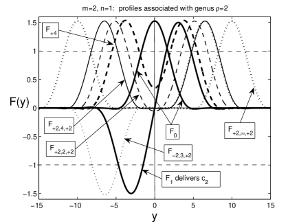
Figure 2. Seven patterns $F(y)$ indicated in Table 1; $m=2$ and $n=1$.

Genus three. Similarly, for $k=3$ (genus $\rho=3$), there are also several patterns that can pretend to deliver the L–S critical value $c_{3}$. These are shown in Figure 3.

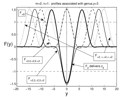
Figure 3. Five patterns $F(y)$ indicated in Table 2; $m=2$ and $n=1$.

The corresponding critical values (3.26) for $n=1$ are shown in Table 2, which allows to conclude as follows:

(3.28) $$\mbox{$k=3$: the S--L critical value $c_{3}=2.0710...$ is again delivered by the basic $F_{2}$}.$$

All critical values in Table 2 are very close to each other. Again checking the accuracy of numerics and taking the critical values $c_{1}$ in Table 1 and $c_{F}$ for $F_{+2,\infty,+2,\infty,+2}$ in Table 2, consisting of three independent $F_{0}$’s, yields, to within $10^{-4}$,

$$c_{F}=3^{\frac{2-\beta}{2}}\tilde{H}(v_{0})=3^{\frac{1}{4}}c_{1}=1.31607...\times 1.6203...=2.1324...\,.$$

Table 2. Critical values of $\tilde{H}(v)$; genus three

$F$	$c_{F}$
$F_{2}$	$2.0710...=c_{3}$
$F_{+2,2,+2,2,+2}$	$2.1305...$
$F_{+2,3,-2,3,+2}$	$2.1322...$
$F_{+2,\infty,+2,\infty,+2}$	$2.1324...$
$F_{+6}$	$2.1647...$

Note that the S–L category-genus construction (3.11) itself guarantees that all solutions $\{v_{k}\}$ as critical points will be (geometrically) distinct; see [25, p. 381]. Here we stress upon two important conclusions:

(I) First, what is key for us, is that closed subsets in ${\mathcal{H}}_{0}$ of functions of the sum type in (3.25) do not deliver S–L critical values in (3.11);

(II) On the other hand, patterns of the $\{F_{0},F_{0}\}$-interaction, i.e., those associated with the sum structure as in (3.25) do exist; see Figures 12 for $m=2$; and

(III) Hence, these patterns (different from the basic ones $\{F_{l}\}$) as well as many others are not obtainable by a direct S–L approach. Therefore, we will need another version of S–L and fibering theory, with different type of decomposition of functional spaces to be introduced below.

Genus $k$. Similarly taking a proper sum of shifted and reflected functions $\pm v_{0}(y\pm ly_{0})$, we obtain from (3.11) that

(3.29) $$c_{k-1}<c_{k}\leq k^{\frac{2-\beta}{2}}c_{1}.$$

Conclusions: conjecture and an open problem. As a conclusion, we mention that, regardless such close critical values $c_{F}$, the above numerics confirm that there is a geometric-algebraic way to distinguish the S–L patterns delivering (3.11). It can be seen from (3.26) that, destroying internal oscillatory “tail”, or even any two-three zeros between two $F_{0}$-like patterns in the complicated pattern $F(y)$,

(3.30) decreases two main terms $$-\int|\tilde{D}^{m}F|^{2} \int|F|^{\frac{3}{2}} c_{F}$$ and in in (3.20).

Recall that precisely these terms in the ODE

$$F^{(4)}=-|F|^{-\frac{1}{2}}F+...\quad(\mbox{see (\ref{4.3}) for $n=1$})$$

are responsible for formation of the tail as shown in Section 4, while the $F$-term, giving $\int F^{2}$, is negligible in the tail. Decreasing both terms, i.e., eliminating the tail in between $F_{0}$’s, will decrease the value $c_{F}$, since in (3.20) the numerator gets less and the denominator larger. Therefore, composing a complicated pattern $F_{l}(y)$ from several elementary profiles looking like $F_{0}(y)$, by using $(k-1)$-dimensional manifolds of genus $k$, we follow

Formal Rule of Composition (FRC) of patterns: performing maximization of $\tilde{H}(v)$ of any $(k-1)$-dimensional manifold ${\mathcal{F}}\in{\mathcal{M}}_{k}$,

(3.31) the S–L point $$F_{k-1}(y)$$ is obtained by minimizing all internal tails and zeros,

i.e., making the minimal number of internal transversal zeros between single structures.

Regardless such a simple variational-oscillatory meaning (3.30) of this FRC, we do not know how to give to such a rule a rigorous sounding.

Concerning the actual critical S–L points, we end up with the following conjecture, which well-corresponds to the FRC (3.31):

Conjecture 3.4. For $N=1$ and any $m\geq 2$, the critical S–L value $(\ref{ck1})$, $k\geq 1$, is delivered by the basic pattern $F_{k-1}$, obtained by minimization on the corresponding $(k-1)$-dimensional manifold ${\mathcal{F}}\in{\mathcal{M}}_{k}$, which is the interaction

(3.32) $$F_{k-1}=(-1)^{k-1}\{+F_{0},-F_{0},+F_{0},...,(-1)^{k-1}F_{0}\},$$

where each neighbouring pair $\{F_{0},-F_{0}\}$ or $\{-F_{0},F_{0}\}$ has a single transversal zero in between the structures.

We also would like to formulate the following conclusion that is again associated with the specific structure of the L–S construction (3.11) over suitable subsets ${\mathcal{F}}$ as smooth $(k-1)$-dimensional manifolds of genus $k$:

Open problem 3.5. For $N=1$ and $m\geq 2$, there are no any purely geometric-topology arguments establishing that the conclusion of Conjecture $\ref{SectVar}.4$ holds. Naturally, the same remains true in ${\mathbb{R}}^{N}$.

In other words, we claim that the metric “tail”-analysis of the functionals involved in the FRC (3.31) cannot be dispensed with by any geometric-type arguments. Actually, the geometric analysis is nicely applied for $m=1$ and this is perfectly covered by Sturm’s Theorem on zeros for second-order ODEs. If such a Sturm Theorem is nonexistent, this emphasizes the end of geometry-topology (or purely homotopy if tails are oscillatory) nature of the variational problem under consideration.

On patterns in ${\mathbb{R}}^{N}$. In the elliptic setting in ${\mathbb{R}}^{N}$, such a clear picture of basic patterns $F_{l}(y)$ obtained via (3.11) with $k=l+1$ is not available. As usual in elliptic theory, nodal structure of solutions in ${\mathbb{R}}^{N}$ is very difficult to reveal. Nevertheless, we strongly believe that the L–S minimax approach (3.11) also can be used to detect the geometric shape of patterns in the $N$-dimensional geometry.

For instance, it is most plausible that the 1-dipole profile $F_{1}(y)$, which is not radially symmetric is essentially composed from two radial $F_{0}(y)$-type profiles via an $\{-F_{0},F_{0}\}$-interaction (q.v. Figure 15 in 1D). Therefore, $F_{1}(y)$ has two dominant extrema, in a natural way, similar to the second eigenfunction

(3.33) $$\frac{{\mathrm{d}}}{{\mathrm{d}}y_{1}}\,{\mathrm{e}}^{-|y|^{2}/4}\sim y_{1}{\mathrm{e}}^{-|y|^{2}/4}\quad\mbox{in}\quad{\mathbb{R}}^{N}$$

of the self-adjoint second-order Hermite operator

$$H_{2}=\Delta+\frac{1}{2}\,y\cdot\nabla+\frac{N}{2}\,I.$$

Such a comparison assumes a bifurcation phenomenon at $n=0$ from eigenfunctions of the linearized operator; see applications in [15, Appendix] to second-order quasilinear porous medium operators. Compactification of the pattern (3.33) and making it oscillatory at the interface surface would lead to correct understanding what the 1-dipole profile looks like, at least, for small $n>0$. Similar analogy is developed for all odd patterns $F_{2k+1}$. For instance, $F_{3}(y)$ has a dominant “topology” similar to the fourth eigenfunction of $H_{2}$,

$$\frac{{\mathrm{d}}^{3}}{{\mathrm{d}}y_{1}^{3}}\,{\mathrm{e}}^{-|y|^{2}/4}\sim\frac{y_{1}}{2}\big{(}\frac{y_{1}^{2}}{2}-3\big{)}{\mathrm{e}}^{-|y|^{2}/4},$$

which has precisely four extrema on the $y_{1}$-axis, etc.

Concerning even patterns $F_{2k}$, we believe that the above L–S algorithm leads to simple radially-symmetric solutions of (1.7), i.e., solutions of ODEs; see further comments below.

Remark: on radial and 1D geometry. Of course, the elliptic equation (1.7) also admits a countable family of radially symmetric solutions

$$\{F_{l}^{\rm rad}(|y|),\,l=0,2,4,...\}$$

satisfying the corresponding ODE. These are constructed in a similar manner by L–S and fibering theory. In 1D, this gives the basic set $\{F_{l}^{\rm 1D},\,l=0,1,2,...\}$ that was described in the previous sections. We expect that the first members of all three families coincide,

(3.34) $$F_{0}=F_{0}^{\rm rad}=F_{0}^{\rm 1D}.$$

Further correspondence of the L–S spectrum of patterns in Proposition 3.2 and the 1D one $\{F_{l}^{\rm 1D},\,l\geq 0\}$ is discussed in [18, § 4].

4. Problem “Oscillations”: local oscillatory structure of solutions close to interfaces and periodic connections with singularities

As we have seen, the first principal feature of the ODEs (1.8) (and the elliptic counterparts) is that these admit compactly supported solutions. Indeed, all interesting for us patterns have finite interfaces. This has been proved in Proposition 3.1 in a general elliptic setting.

Therefore, we are going to study typical local behaviour of the solutions of (1.8) close to the singular points, i.e., to finite interfaces. We will reveal extremely oscillatory structure of such behaviour to be compared with global oscillatory behaviour obtained above by variational techniques.

The phenomenon of oscillatory changing sign behaviour of solutions of the Cauchy problem has been detected for various classes of evolution PDEs; see a general view in [20, Ch. 3-5] and various results for different PDEs in [11, 12, 13]. For the present $2m$th-order equations, the oscillatory behaviour exhibits special features to be revealed. We expect that the presented oscillation analysis makes sense for more general solutions of the parabolic equation (1.1) and explains their generic behaviour close to the moving interfaces.

4.1. Autonomous ODEs for oscillatory components

Assume that the finite interface of $F(y)$ is situated at the origin $y=0$, so that we can use the trivial extension $F(y)\equiv 0$ for $y<0$. We then are interested in describing the behaviour of solutions as $y\to 0^{+}$, so we consider the ODE (1.8) written in the form

(4.1) $$F^{(2m)}=(-1)^{m+1}|F|^{-\alpha}F+(-1)^{m}F\,\,\,\mbox{for}\,\,y>0,\,\,\,F(0)=0\quad\big{(}\alpha=\frac{n}{n+1}\in(0,1)\big{)}.$$

In view of the scaling structure of the first two terms, for convenience, we perform extra rescaling and introduce the oscillatory component $\varphi(s)$ of $F$ by

(4.2) $$F(y)=y^{\gamma}\varphi(s),\quad\mbox{where}\quad s=\ln y\quad\mbox{and}\quad\gamma=\frac{2m}{\alpha}\equiv\frac{2m(n+1)}{n}.$$

Therefore, since $s\to-\infty$ (the new interface position) as $y\to 0^{-}$, the monotone function $y^{\gamma}$ in (4.2) plays the role of the envelope to the oscillatory function $F(y)$. Substituting (4.2) into (4.1) yields the following equation for $\varphi$:

(4.3) $$P_{2m}(\varphi)=(-1)^{m+1}|\varphi|^{-\alpha}\varphi+(-1)^{m}{\mathrm{e}}^{2ms}\varphi.$$

Here $\{P_{k},\,k\geq 0\}$ are linear differential operators defined by the recursion

(4.4) $$P_{k+1}(\varphi)=(P_{k}(\varphi))^{\prime}+(\gamma-k)P_{k}(\varphi)\,\,\,\mbox{for}\,\,\,k=0,1,...\,,\,\,\,P_{0}(\varphi)=\varphi.$$

Let us present the first five operators, which are sufficient for further use:

$$P_{1}(\varphi)=\varphi^{\prime}+\gamma\varphi;$$

$$P_{2}(\varphi)=\varphi^{\prime\prime}+(2\gamma-1)\varphi^{\prime}+\gamma(\gamma-1)\varphi;$$

$$P_{3}(\varphi)=\varphi^{\prime\prime\prime}+3(\gamma-1)\varphi^{\prime\prime}+(3\gamma^{2}-6\gamma+2)\varphi^{\prime}+\gamma(\gamma-1)(\gamma-2)\varphi;$$

(4.5) $$P_{4}(\varphi)=\varphi^{(4)}+2(2\gamma-3)\varphi^{\prime\prime\prime}+(6\gamma^{2}-18\gamma+11)\varphi^{\prime\prime}\vskip 3.0pt plus 1.0pt minus 1.0pt$$

$$\qquad\quad\,\,+2(2\gamma^{3}-9\gamma^{2}+11\gamma-3)\varphi^{\prime}+\gamma(\gamma-1)(\gamma-2)(\gamma-3)\varphi;\vskip 3.0pt plus 1.0pt minus 1.0pt$$

$$P_{5}(\varphi)=\varphi^{(5)}+5(\gamma-2)\varphi^{(4)}+5(2\gamma^{2}-8\gamma+7)\varphi^{\prime\prime\prime}+5(\gamma-2)(2\gamma^{2}-8\gamma+5)\varphi^{\prime\prime}\vskip 3.0pt plus 1.0pt minus 1.0pt$$

$$\qquad\quad\,\,+(5\gamma^{4}-40\gamma^{3}+105\gamma^{2}-100\gamma+24)\varphi^{\prime}+\,\gamma(\gamma-1)(\gamma-2)(\gamma-3)(\gamma-4)\varphi;\,\,\,\mbox{etc.}$$

According to (4.2), the interface at $y=0$ now corresponds to $s=-\infty$, so that (4.3) is an exponentially (as $s\to-\infty$) perturbed autonomous ODE

(4.6) $$P_{2m}(\varphi)=(-1)^{m+1}|\varphi|^{-\alpha}\varphi\quad\mbox{in}\quad{\mathbb{R}}\quad\big{(}\alpha=\frac{n}{n+1}\big{)},$$

which we will concentrate upon. By classic ODE theory [8], one can expect that for $s\ll-1$ typical (generic) solutions of (4.3) and (4.6) asymptotically differ by exponentially small factors. Of course, we must admit that (4.6) is a singular ODE with a non-Lipschitz term, so the results on continuous dependence need extra justification in general.

Thus, in two principal cases, the ODEs for the oscillatory component $\varphi(s)$ are

(4.7) $$m=2:\quad P_{4}(\varphi)=-|\varphi|^{-\alpha}\varphi,$$

(4.8) $$m=3:\quad P_{6}(\varphi)=+|\varphi|^{-\alpha}\varphi,$$

that exhibit rather different properties because comprise even and odd $m$’s. For instance, (4.6) for any odd $m\geq 1$ (including (4.8)) has two constant equilibria, since

(4.9) $$\begin{matrix}\gamma(\gamma-1)...(\gamma-(2m-1))\varphi=|\varphi|^{-\alpha}\varphi\quad\Longrightarrow\vskip 3.0pt plus 1.0pt minus 1.0pt\\ \varphi(s)=\pm\varphi_{0}\equiv\pm[\gamma(\gamma-1)...(\gamma-(2m-1))]^{-\frac{1}{\alpha}}\quad\mbox{for all \, $n>0$}.\end{matrix}$$

For even $m$ including (4.7), such equilibria for (4.6) do not exist at least for $n\in(0,1]$. We will show how this affects the oscillatory properties of solutions for odd and even $m$’s.

4.2. Periodic oscillatory components

We now look for periodic solutions of (4.6), which are the simplest nontrivial bounded solutions that can be continued up to the interface at $s=-\infty$. Periodic solutions together with their stable manifolds are simple connections with the interface, as a singular point of the ODE (1.8).

Note that (4.6) does not admit variational setting, so we cannot apply well developed potential [28, Ch. 8] (see a large amount of related existence-nonexistence results and further references therein), or degree [24, 25] theory. For $m=2$, the proof of existence of $\varphi_{*}$ can be done by shooting; see [11, § 7.1] that can be extended to $m=3$ as well. Nevertheless, uniqueness of a periodic orbit is still open, so we conjecture the following result supported by various numerical and analytical evidence (cf. [20, § 3.7]):

Conjecture 4.1. For any $m\geq 2$ and $\alpha\in(0,1]$, the ODE $(\ref{2.4})$ admits a unique nontrivial periodic solution $\varphi_{*}(s)$ of changing sign.

4.3. Numerical construction of periodic orbits for $m=2$

Numerical results clearly suggest that (4.7) possesses a unique periodic solution $\varphi_{*}(s)$, which is stable in the direction opposite to the interface, i.e., as $s\to+\infty$; see Figure 4. The proof of exponential stability and hyperbolicity of $\varphi_{*}$ is straightforward by estimating the eigenvalues of the linearized operator. This agrees with the obviously correct similar result for $n=0$, namely, for the linear equation (4.1) for $\alpha=0$

(4.10) $$F^{(4)}=-F\quad\mbox{as}\quad y\to-\infty.$$

Here the interface is infinite, so its position corresponds to $y=-\infty$. Indeed, setting $F(y)={\mathrm{e}}^{\mu y}$ gives the characteristic equation and a unique exponentially decaying pattern

(4.11) $$\mu^{4}=-1\quad\Longrightarrow\quad\mbox{$F(y)\sim{\mathrm{e}}^{\frac{y}{\sqrt{2}}}\,\,\bigl{[}A\cos\bigl{(}\frac{y}{\sqrt{2}}\bigr{)}+B\sin\bigl{(}\frac{y}{\sqrt{2}}\bigr{)}\bigr{]}\,\,\,\mbox{as}\,\,\,y\to-\infty.$}$$

Continuous dependence on $n\geq 0$ of typical solutions of (4.6) with “transversal” zeros only will continue to be key in our analysis, that actually means existence of a “homotopic” connection between the nonlinear and the linear ($n=0$) equations. The passage to the limit $n\to 0$ in similar degenerate ODEs from thin film equations (TFEs) theory is discussed in [11, § 7.6].

The oscillation amplitude becomes very small for $n\approx 0$, so we perform extra scaling.

Limit ${n\to 0}$. This scaling is

(4.12) $$\varphi(s)=\bigl{(}\frac{n}{4}\bigr{)}^{\frac{4}{n}}\Phi(\eta),\quad\mbox{where}\quad\eta=\frac{4s}{n},$$

where $\Phi$ solves a simpler limit binomial ODE,

(4.13) $${\mathrm{e}}^{-\eta}({\mathrm{e}}^{\eta}\Phi)^{(4)}\equiv\Phi^{(4)}+4\Phi^{\prime\prime\prime}+6\Phi^{\prime\prime}+4\Phi^{\prime}+\Phi=-\big{|}\Phi\big{|}^{-\frac{n}{n+1}}\Phi.$$

The stable oscillatory patterns of (4.13) are shown in Figure 5. For such small $n$ in Figure 5(a) and (b), by scaling (4.12), the periodic components $\varphi_{*}$ get really small, e.g.,

$$\begin{matrix}\max|\varphi_{*}(s)|\sim 3\cdot 10^{-4}\bigl{(}\frac{n}{4}\bigr{)}^{\frac{4}{n}}\sim 3\cdot 10^{-30}\quad\mbox{for \,\, $n=0.2$ \,in \,(a)},\vskip 3.0pt plus 1.0pt minus 1.0pt\vskip 3.0pt plus 1.0pt minus 1.0pt\\ \mbox{and}\quad\max|\varphi_{*}(s)|\sim 10^{-93}\quad\mbox{for \,\, $n=0.08$ \,in \,(b)}.\end{matrix}$$

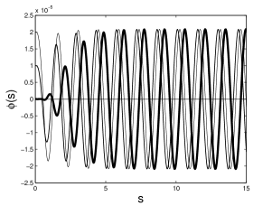
(a) $n=2$

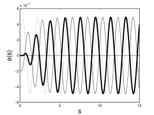
(b) $n=4$

Figure 4. Convergence to the stable periodic solution of (4.7) for $n=2$ (a) and $n=4$ (b).

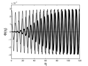
(a) $n=0.2$

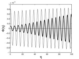
(b) $n=0.08$

Figure 5. Stable periodic oscillations in the ODE (4.13) for $n=0.2$ (a) and $n=0.08$ (b).

Limit ${n\to\infty}$. Then $\alpha\to 1$, so the original ODE (4.7) approaches the following equation with a discontinuous sign-nonlinearity:

(4.14) $$\varphi_{\infty}^{(4)}+10\varphi_{\infty}^{\prime\prime\prime}+35\varphi_{\infty}^{\prime\prime}+50\varphi_{\infty}^{\prime}+24\varphi_{\infty}=-{\rm sign}\,\varphi_{\infty}.$$

This also admits a stable periodic solution, as shown in Figure 6.

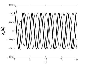
Figure 6. Convergence to the stable periodic solution of (4.14) ($n=+\infty$).

4.4. Numerical construction of periodic orbits for $m=3$

Consider now equation (4.8) that admits constant equilibria (4.9) existing for all $n>0$. It is easy to check that the equilibria $\pm\varphi_{0}$ are asymptotically stable as $s\to+\infty$. Then the necessary periodic orbit is situated in between of these stable equilibria, so it is unstable as $s\to+\infty$.

Such an unstable periodic solution of (4.8) is shows in Figure 7 for $n=15$, which is obtained by shooting from $s=0$ with prescribed Cauchy data.

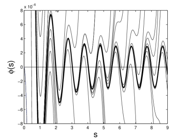
Figure 7. Unstable periodic behavior of the ODE (4.8) for $n=15$. Cauchy data are given by $\varphi(0)=10^{-4}$, $\varphi^{\prime}(0)=\varphi^{\prime\prime\prime}(0)=...=\varphi^{(5)}(0)=0$, and $\varphi^{\prime\prime}(0)=-5.0680839826093907...\times 10^{-4}$ .

As for $m=2$, in order to reveal periodic oscillations for smaller $n$ (actually, there is a numerical difficulty already for $n\leq 4$), we apply the scaling

(4.15) $$\varphi(s)=\bigl{(}\frac{n}{6}\bigr{)}^{\frac{6}{n}}\Phi(\eta),\quad\mbox{where}\quad\eta=\frac{6s}{n}.$$

This gives in the limit a simplified ODE with the binomial linear operator,

(4.16) $${\mathrm{e}}^{-\eta}({\mathrm{e}}^{\eta}\Phi)^{(6)}\equiv\Phi^{(6)}+6\Phi^{(5)}+15\Phi^{(4)}+20\Phi^{\prime\prime\prime}+15\Phi^{\prime\prime}+6\Phi^{\prime}+\Phi=\big{|}\Phi\big{|}^{-\frac{n}{n+1}}\Phi.$$

Figure 8 shows the trace of the periodic behaviour for equation (4.16) with $n=\frac{1}{2}$. According to scaling (4.15), the periodic oscillatory component $\varphi_{*}(s)$ gets very small,

$$\max|\varphi_{*}|\sim 1.1\times 10^{-18}\,\,\,\mbox{for}\,\,\,n=0.5.$$

A more detailed study of the behaviour of the oscillatory component as $n\to 0$ is available in [12, § 12].

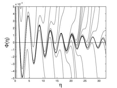
Figure 8. Unstable periodic behavior of the ODE (4.16) for $n=\frac{1}{2}$. Cauchy data are given by $\varphi(0)=10^{-4}$, $\varphi^{\prime}(0)=\varphi^{\prime\prime\prime}(0)=...=\varphi^{(5)}(0)=0$, and $\varphi^{\prime\prime}(0)=-9.456770333415...\times 10^{-4}$ .

The passage to the limit $n\to+\infty$ leads to the equation with discontinuous nonlinearity that is easily obtained from (4.8). This admits a periodic solution, which is rather close to the periodic orbit in Figure 7 obtained for $n=15$.

We claim that the above two cases $m=2$ (even) and $m=3$ (odd) exhaust all key types of periodic behaviours in ODEs like (1.8). Namely, periodic orbits are stable for even $m$ and are unstable for odd, with typical stable and unstable manifolds as $s\to\pm\infty$. So we observe a dichotomy relative to all orders $2m$ of the ODEs under consideration.

5. Problem “Numerics”: numerical construction and first classification of basic types of localized blow-up or compacton patterns for $m=2$

We need a careful numerical description of various families of solutions of the ODEs (1.8). In practical computations, we have to use the regularized version of the equations,

(5.1) $$(-1)^{m}F^{(2m)}=F-\big{(}\varepsilon^{2}+F^{2}\big{)}^{-\frac{n}{2(n+1)}}F\quad\mbox{in}\,\,\,{\mathbb{R}},$$

which, for $\varepsilon>0$, contains smooth analytic nonlinearities. In numerical analysis, we typically take $\varepsilon=10^{-4}$ or, at least, $10^{-3}$ which is sufficient to revealing global structures.

It is worth mentioning that detecting in Section 4 a highly oscillatory structure of solutions close to interfaces makes it impossible to use well-developed homotopy theory [22, 41] that was successfully applied to another class of fourth-order ODEs with coercive operators; see also Peletier–Troy [29]. Roughly speaking, our non-smooth problem cannot be used in a homotopy classification, since the oscillatory behaviour close to interfaces destroys such a standard homotopy parameter as the number of rotations on the hodograph plane $\{F,F^{\prime}\}$. Indeed, for any solution of (1.8), the rotation number about the origin is always infinite. Then as $F\to 0$, i.e., as $y\to\pm\infty$, the linearized equation is (4.10), which admits the oscillatory behaviour (4.11).

5.1. Fourth-order equation: $m=2$

We will describe main families of solutions.

First basic pattern and structure of zeros. For $m=2$, (1.8) reads

(5.2) $$F^{(4)}=F-\big{|}F\big{|}^{-\frac{n}{n+1}}F\quad\mbox{in}\,\,\,{\mathbb{R}}.$$

We are looking for compactly supported patterns $F$ (see Proposition 3.1) satisfying

(5.3) $$\begin{matrix}{\rm meas}\,{\rm supp}\,\,F>2R_{*},\quad\mbox{where $R_{*}>\frac{\pi}{2}$ is the first}\vskip 3.0pt plus 1.0pt minus 1.0pt\vskip 3.0pt plus 1.0pt minus 1.0pt\\ \mbox{ positive root of the equation \,\,$\tanh R=-\tan R$.}\end{matrix}$$

In Figure 9, we show the first basic pattern called the $F_{0}(y)$ for various $n\in[\frac{1}{10},100]$. Concerning the last profile $n=100$, note that (5.2) admits a natural passage to the limit $n\to+\infty$ that gives the ODE with a discontinuous nonlinearity,

(5.4) $$F^{(4)}=F-{\rm sign}\,F\equiv\left\{\begin{matrix}F-1\quad\,\,\,\,\mbox{for}\quad F>0,\vskip 3.0pt plus 1.0pt minus 1.0pt\\ F+1\quad\mbox{for}\quad F<0.\end{matrix}\right.$$

A unique oscillatory solution of (5.4) can be treated by an algebraic approach; cf. [11, § 7.4]. For $n=1000$ and $n=+\infty$, the profiles are close to that for $n=100$ in Figure 9.

The profiles in Figure 9 are constructed by MATLAB with extra accuracy, where $\varepsilon$ in (5.1) and both tolerances in the bvp4c solver have been enhanced and took the values $\varepsilon=10^{-7}$ and ${\rm Tols}=10^{-7}.$ This allows us also to check the refined local structure of multiple zeros at the interfaces. Figure 10 corresponding to $n=1$ explains how the zero structure repeats itself from one zero to another in the usual linear scale.

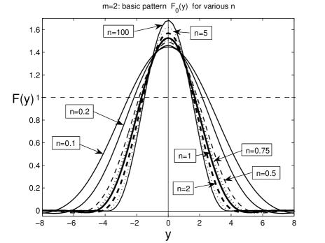
Figure 9. The first (stable) solution $F_{0}(y)$ of (5.2) for various $n$.

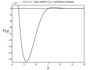
(a) scale $10^{-3}$

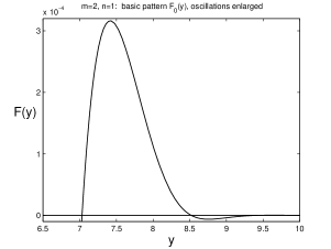
(b) scale $10^{-4}$

Figure 10. Enlarged zero structure of the profile $F_{0}(y)$ for $n=1$ in the linear scale.

Basic countable family: approximate Sturm’s property. In Figure 11, we show the basic family denoted by $\{F_{l},\,l=0,1,2,...\}$ of solutions of (5.2) for $n=1$. Each profile $F_{l}(y)$ has precisely $l+1$ “dominant” extrema and $l$ “transversal” zeros; see further discussion below and [16, § 4] for other details. It is important that all the internal zeros of $F_{l}(y)$ are clearly transversal (obviously, excluding the oscillatory end points of the support). In other words, each profile $F_{l}$ is approximately obtained by a simple “interaction” (gluing together) of $l+1$ copies of the first pattern $\pm F_{0}$ taking with necessary signs; see further development below.

Actually, if we forget for a moment about the complicated oscillatory structure of solutions near interfaces, where an infinite number of extrema and zeros occur, the dominant geometry of profiles in Figure 11 looks like it approximately obeys Sturm’s classic zero set property, which is true rigorously for $m=1$ only, i.e., for the second-order ODE

(5.5) $$F^{\prime\prime}=-F+\big{|}F\big{|}^{-\frac{n}{n+1}}F\quad\mbox{in}\quad{\mathbb{R}}.$$

For (5.5), the basic family $\{F_{l}\}$ is constructed by direct gluing together the explicit patterns (1.5), i.e., $\pm F_{0}$. Therefore, each $F_{l}$ consists of precisely $l+1$ patterns (1.5) (with signs $\pm F_{0}$), so that Sturm’s property is clearly true. In Section 3, we presented some analytic evidence showing that precisely this basic family $\{F_{l}\}$ is obtained by direct application of L–S category theory.

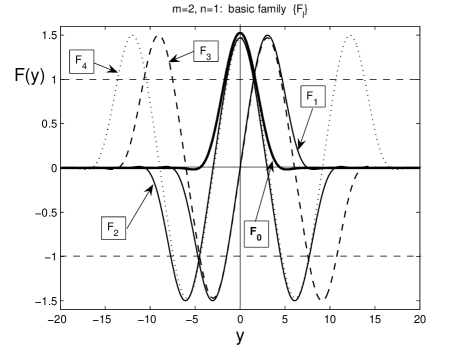
Figure 11. The first five patterns of the basic family $\{F_{l}\}$ of the ODE (5.2) for $n=1$.

5.2. Countable family of $\{F_{0},F_{0}\}$-interactions

We now show that the actual nonlinear interaction of the two first patterns $+F_{0}(y)$ leads to a new family of profiles.

In Figure 12, $n=1$, we show the first profiles from this family denoted by $\{F_{+2,k,+2}\}$, where in each function $F_{+2,k,+2}$ the multiindex $\sigma=\{+2,k,+2\}$ means, from left to right, +2 intersections with the equilibrium +1, then next $k$ intersections with zero, and final +2 stands again for 2 intersections with +1. Later on, we will use such a multiindex notation to classify other patterns obtained.

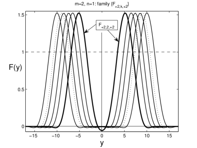
Figure 12. First patterns from the family $\{F_{+2,k,+2}\}$ of the $\{F_{0},F_{0}\}$-interaction; $n=1$.

In Figure 13, we present the enlarged behaviour of zeros explaining the structure of the interior layer of connection of two profiles $\sim+F_{0}(y)$. In particular, (b) shows that there exist two profiles $F_{+2,6,+2}$, these are given by the dashed line and the previous one, both having two zeros on $[-1,1]$. Therefore, the identification and the classification of the profiles just by the successive number of intersections with equilibria 0 and $\pm 1$ is not always acceptable (in view of a non-homotopic nature of the problem), and some extra geometry of curves near intersections should be taken into account. In fact, precisely this proves that a standard homotopy classification of patterns is not consistent for such non-coercive and oscillatory equations. Anyway, whenever possible without confusion, we will continue use such a multiindex classification, though now meaning that in general a profile $F_{\sigma}$ with a given multiindex $\sigma$ may denote actually a class of profiles with the given geometric characteristics. Note that the last profile in Figure 12 is indeed $F_{+2,6,+2}$, where the last two zeros are seen in the scale $\sim 10^{-6}$ in Figure 14. Observe here a clear non-smoothness of two last profiles as a numerical discrete mesh phenomenon, which nevertheless does nor spoil at all this differential presentation.

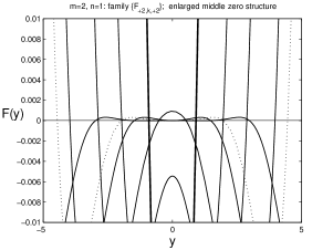
(a) zeros: scale $10^{-2}$

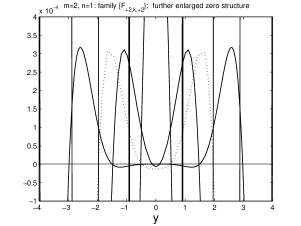
(b) zeros: scale $10^{-4}$

Figure 13. Enlarged middle zero structure of the profiles $F_{+2,k,+2}$ from Figure 12.

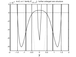
Figure 14. Enlarged middle zero structure of the profiles $F_{+2,6,+2}$ from Figure 12.

In view of the oscillatory character of $F_{0}(y)$ at the interfaces, we expect that the family $\{F_{+2,k,+2}\}$ is countable, and such functions exist for any even $k=0,2,4,...\,$. Then $k=+\infty$ corresponds to the non-interacting pair

(5.6) $$F_{0}(y+y_{0})+F_{0}(y-y_{0}),\quad\mbox{where}\,\,\,\,\,{\rm supp}\,F_{0}(y)=[-y_{0},y_{0}].$$

Of course, there exist various triple $\{F_{0},F_{0},F_{0}\}$ and any multiple interactions $\{F_{0},...,F_{0}\}$ of $k$ single profiles, with different distributions of zeros between any pair of neighbours.

5.3. Countable family of $\{-F_{0},F_{0}\}$-interactions

We now describe the interaction of $-F_{0}(y)$ with $F_{0}(y)$. In Figure 15, $n=1$, we show the first profiles from this family denoted by $\{F_{-2,k,+2}\}$, where for the multiindex $\sigma=\{-2,k,+2\}$, the first number $-2$ means 2 intersections with the equilibrium $-1$, etc. The zero structure close to $y=0$ is presented in Figure 16. It follows from (b) that the first two profiles belong to the class $F_{-2,1,2},$ i.e., both have a single zero for $y\approx 0$. The last solution shown is $F_{-2,5,+2}$. Again, we expect that the family $\{F_{-2,k,+2}\}$ is countable, and such functions exist for any odd $k=1,3,5,...$, and $k=+\infty$ corresponds to the non-interacting pair

(5.7) $$-F_{0}(y+y_{0})+F_{0}(y-y_{0})\quad\bigl{(}{\rm supp}\,F_{0}(y)=[-y_{0},y_{0}]\bigr{)}.$$

There exist families of an arbitrary number of interactions such as $\{\pm F_{0},\pm F_{0},...,\pm F_{0}\}$ consisting of any $k\geq 2$ members.

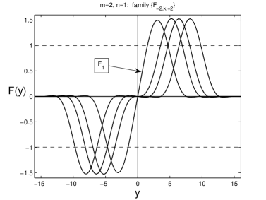
Figure 15. First four patterns from the family $\{F_{-2,k,+2}\}$ of the $\{-F_{0},F_{0}\}$-interactions; $n=1$.

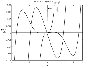
(a) zeros: scale $10^{-2}$

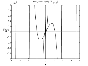
(b) zeros: scale $10^{-4}$

Figure 16. Enlarged middle zero structure of the profiles $F_{-2,k,+2}$ from Figure 15.

5.4. Periodic solutions in ${\mathbb{R}}$

Before introducing new types of patterns, we need to describe other non-compactly supported solutions in ${\mathbb{R}}$. As a variational problem, equation (5.2) admits an infinite number of periodic solutions; see e.g. [28, Ch. 8]. In Figure 17 for $n=1$, we present a special unstable periodic solution obtained by shooting from the origin with conditions

$$F(0)=1.5,\quad F^{\prime}(0)=F^{\prime\prime\prime}(0)=0,\quad F^{\prime\prime}(0)=-0.3787329255...\,.$$

We will show next that precisely the periodic orbit $F_{*}(y)$ with

(5.8) $$F_{*}(0)\approx 1.535...$$

plays an important part in the construction of other families of compactly supported patterns. Namely, all the variety of solutions of (5.2) that have oscillations about equilibria $\pm 1$ are close to $\pm F_{*}(y)$ there.

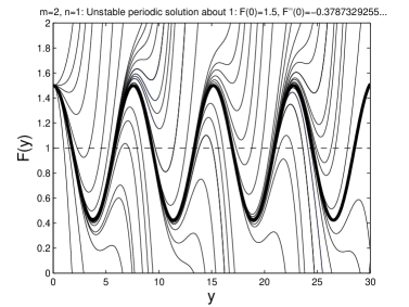
Figure 17. An example of a periodic solution of the ODE (5.2) for $n=1$.

5.5. Family $\{F_{+2k}\}$

Such functions $F_{+2k}$ for $k\geq 1$ have $2k$ intersection with the single equilibrium +1 only and have a clear “almost” periodic structure of oscillations about; see Figure 18(a). The number of intersections denoted by $+2k$ gives an extra Strum index to such a pattern. In this notation, $F_{+2}=F_{0}.$

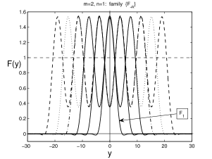
(a) $F_{+2k}(y)$

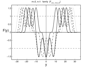
(b) $F_{+k,l,-m,l,+k}$

Figure 18. Two families of solutions of (5.2) for $n=1$; $F_{+2k}(y)$ (a) and $F_{+k,l,-m,l,+k}$ (b).

5.6. More complicated patterns: towards chaotic structures

Using the above rather simple families of patterns, we claim that a pattern (possibly, a class of patterns) with an arbitrary multiindex of any length

(5.9) $$\sigma=\{\pm\sigma_{1},\sigma_{2},\pm\sigma_{3},\sigma_{4},...,\pm\sigma_{l}\}$$

can be constructed. Figure 18(b) shows several profiles from the family with the index $\sigma=\{+k,l,-m,l,+k\}.$ In Figure 19, we show further four different patterns, while in Figure 20, a single most complicated pattern is presented, for which

(5.10) $$\sigma=\{-8,1,+4,1,-10,1,+8,1,3,-2,2,-8,2,2,-2\}.$$

All computations are performed for $n=1$ as usual. Actually, we claim that the multiindex (5.9) can be arbitrary and takes any finite part of any non-periodic fraction. Actually, this means chaotic features of the whole family of solutions $\{F_{\sigma}\}$. These chaotic types of behaviour are known for other fourth-order ODEs with coercive operators, [29, p. 198].

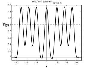
(a) $\sigma=\{+6,2,+2,2,+6\}$

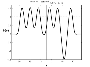
(b) $\sigma=\{+6,2,+4,1,-2,1+2\}$

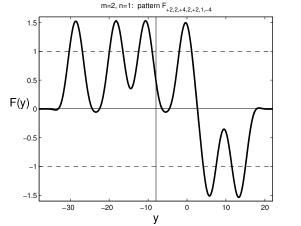
(c) $\sigma=\{+2,2,+4,2,+2,1,-4\}$

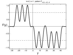
(d) $\sigma=\{+6,3,-4,2,-6\}$

Figure 19. Various patterns for (5.2) for $n=1$.

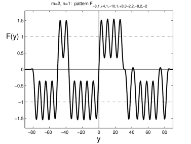
Figure 20. A complicated pattern $F_{\sigma}(y)$ for (5.2) for $n=1$.

6. Problem “Numerics”: patterns in 1D in higher-order cases, $m\geq 3$

The main features of the pattern classification by their structure and computed critical values for $m=2$ in the previous section can be extended to arbitrary $m\geq 3$ in the ODEs (1.8) for $N=1$, so we perform this in less detail.

In Figure 21, for the purpose of comparison, we show the first basic pattern $F_{0}(y)$ for $n=1$ in four main cases $m=1$ (the only non-negative profile by the Maximum Principle known from the 1970s [38], [37, Ch. 4]), and 2, 3, 4. Next Figure 22 explains the oscillatory properties close to the interface. It turns out that, for $m=4$, the solutions are most oscillatory, so we it is convenient to use this case for illustrations.

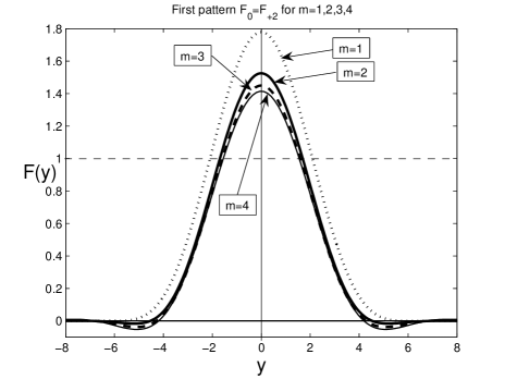
Figure 21. The first solution $F_{0}(y)$ of (1.8), $N=1$, $n=1$, for $m=1,2,3,4$.

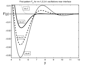
(a) scale $10^{-2}$

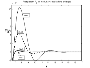
(b) scale $10^{-3}$

Figure 22. Enlarged zero structure of the profile $F_{0}(y)$ for $n=1$ from Figure 21; the linear scale.

In the log-scale, the zero structure is shown in Figure 23 for $m=2,3$, and 4 ($n=1$). For $m=4$ and $m=3$, this makes it possible to observe a dozen of oscillations that well correspond to the oscillatory component analytic formulae (4.2) close to interfaces. For the less oscillatory case $m=2$, we observe 4 reliable oscillations up to $10^{-10}$, which is our best accuracy achieved.

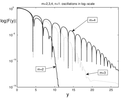
Figure 23. Behaviour of $F_{0}(y)$ for $n=1$, for $m=2,3,4$; the log-scale.

The basic countable family satisfying approximate Sturm’s property has the same topology as for $m=2$ in Section 5, and we do not present such numerical illustrations.

In Figure 24 for $m=3$ and $n=1$, we show the first profiles from the family $\{F_{+2k}\}$, while Figure 25 explains typical structures of $F_{+2,k,+2}\}$ for $m=4$, $n=1$. In Figure 26 for $m=4$ and $n=1$, we show the first profiles from the family $\{F_{+2,k,-2}\}$.

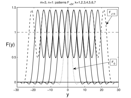
Figure 24. The first seven patterns from the family $\{F_{+2k}\}$; $m=3$ and $n=1$.

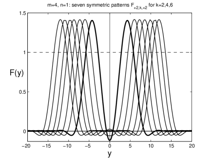
Figure 25. The first patterns from the family $\{F_{+2,k,+2}\}$ of the $\{F_{0},F_{0}\}$-interactions; $m=4$ and $n=1$.

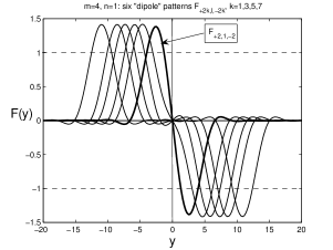
(a) profiles

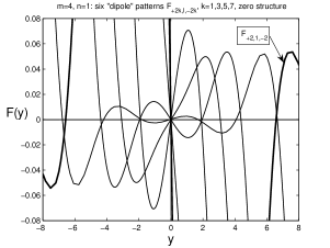
(b) zero structure

Figure 26. The first patterns from the family $\{F_{+2,k,-2}\}$ of the $\{-F_{0},F_{0}\}$-interactions, for $m=4$ and $n=1$: profiles (a), and zero structure (b).

Finally, in Figure 27, for comparison, we present a complicated pattern for $m=3$ and $4$ (the bold line), $n=1$, with the index

(6.1) $$\sigma=\{-8,3,+4,k,-10,1,+8,l,-12\}.$$

Both numerical experiments were performed starting with the same initial data. As a result, we obtain quite similar patterns, with the only difference that, in (6.1), $k=1$, $l=3$ for $m=3$, and for more oscillatory case $m=4$, the number of zeros increase, so now $k=3$ and $l=5$.

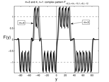
Figure 27. A complicated pattern $F_{\sigma}(y)$ for $m=3,4$ and $n=1$.

Our study of other key aspects of these challenging elliptic problems will be soon continued in [18].

References

- [1] A. Bahri and H. Berestycki, A perturbation method in critical point theory and applications, Trans. Amer. Math. Soc., 267 (1981), 1–32.
- [2] A. Bahri and P.L. Lions, Morse index in some min–max critical points. I. Application to multiplicity results, Comm. Pure Appl. Math., XLI (1988), 1027–1037.
- [3] M. Berger, Nonlinearity and Functional Analysis, Acad. Press, New York, 1977.
- [4] T. Boggio, Sull’equilibrio delle piastre elastiche incastrate, Rend. Acc. Lincei, 10 (1901), 197–205.
- [5] T. Boggio, Sulle funzioni di Green d’ordine , Rend. Circ. Mat. Palermo, 20 (1905), 97–135.
- [6] H. Brezis and F. Brawder, Partial Differential Equations in the 20th Century, Adv. in Math., 135 (1998), 76–144.
- [7] D.C. Clark, A variant of Lusternik–Schnirelman theory, Indiana Univ. Math. J., 22 (1972), 65–74.
- [8] E.A. Coddington and N. Levinson, Theory of Ordinary Differential Equations, McGraw-Hill Book Company, Inc., New York/London, 1955.
- [9] K. Deimling, Nonlinear Functional Analysis, Springer-Verlag, Berlin/Tokyo, 1985.
- [10] U. Elias, Eigenvalue problems for the equation , J. Differ. Equat., 29 (1978), 28–57.
- [11] J.D. Evans, V.A. Galaktionov, and J.R. King, Source-type solutions of the fourth-order unstable thin film equation, Euro J. Appl. Math., 18 (2007), 273–321.
- [12] J.D. Evans, V.A. Galaktionov, and J.R. King, Unstable sixth-order thin film equation. I. Blow-up similarity solutions; II. Global similarity patterns, Nonlinearity, 20 (2007), 1799–1841, 1843–1881.
- [13] V.A. Galaktionov, On interfaces and oscillatory solutions of higher-order semilinear parabolic equations with nonlipschitz nonlinearities, Stud. Appl. Math., 117 (2006), 353–389.
- [14] V.A. Galaktionov, Nonlinear dispersion equations: smooth deformations, compactons, and extensions to higher orders, Comput. Math. Math. Phys., 48 (2008), 1823–1856 (arXiv:0902.0275).
- [15] V.A. Galaktionov and P.J. Harwin, On evolution completeness of nonlinear eigenfunctions for the porous medium equation in the whole space, Advances Differ. Equat., 10 (2005), 635–674.
- [16] V.A. Galaktinov abd P.J. Harwin, Non-uniqueness and global similarity solutions for a higher-order semilinear parabolic equation, Nonlinearity, 18 (2005), 717–746.
- [17] V.A. Galaktionov, E. Mitidieri, and S.I. Pohozaev, Variational approach to complicated similarity solutions of higher-order nonlinear evolution partial differential equations, In: Sobolev Spaces in Mathematics. II, Appl. Anal. and Part. Differ. Equat., Series: Int. Math. Ser., Vol. 9, V. Maz’ya Ed., Springer, 2009.
- [18] V.A. Galaktionov, E. Mitidieri, and S.I. Pohozaev, Variational approach to complicated similarity solutions of higher-order nonlinear PDEs. II, in preparation (will be available in arXiv.org).
- [19] V.A. Galaktionov and S.I. Pohozaev, Third-order nonlinear dispersion equations: shocks, rarefaction, and blowup waves, Comput. Math. Math. Phys., 48 (2008), 1784–1810 (arXiv:0902.0253).
- [20] V.A. Galaktionov and S.R. Svirshchevskii, Exact Solutions and Invariant Subspaces of Nonlinear Partial Differential Equations in Mechanics and Physics, ChapmanHall/CRC, Boca Raton, Florida, 2007.
- [21] J.K. Hale, Asymptotic Behavior of Dissipative Systems, AMS, Providence, RI, 1988.
- [22] W.D. Kalies, J. Kwapisz, J.B. VandenBerg, and R.C.A.M. VanderVorst, Homotopy classes for stable periodic and chaotic patterns in fourth-order Hamiltonian systems, Commun. Math. Phys., 214 (2000), 573–592.
- [23] S. Kawamoto, An exact transformation from the Harry Dym equation to the modified KdV equation, J. Phys. Soc. Japan, 54 (1985), 2055–2056.
- [24] M.A. Krasnosel’skii, Topological Methods in the Theory of Nonlinear Integral Equations, Pergamon Press, Oxford/Paris, 1964.
- [25] M.A. Krasnosel’skii and P.P. Zabreiko, Geometrical Methods of Nonlinear Analysis, Springer-Verlag, Berlin/Tokyo, 1984.
- [26] J.L. Lions, Quelques méthodes de résolution des problèmes aux limites non linéaires, Dunod, Gauthier–Villars, Paris, 1969.
- [27] V.G. Maz’ja, Sobolev Spaces, Springer-Verlag, Berlin/Tokyo, 1985.
- [28] E. Mitidieri and S.I. Pohozaev, Apriori Estimates and Blow-up of Solutions to Nonlinear Partial Differential Equations and Inequalities, Proc. Steklov Inst. Math., Vol. 234, Intern. Acad. Publ. Comp. Nauka/Interperiodica, Moscow, 2001.
- [29] L.A. Peletier and W.C. Troy, Spatial Patterns: Higher Order Models in Physics and Mechanics, Birkhäuser, Boston/Berlin, 2001.
- [30] S.I. Pohozaev, On an approach to nonlinear equations, Soviet Math. Dokl., 20 (1979), 912–916.
- [31] S.I. Pohozaev, The fibering method in nonlinear variational problems, Pitman Research Notes in Math., Vol. 365, Pitman, 1997, pp. 35–88.
- [32] P. Rabinowitz, Variational methods for nonlinear eigenvalue problems, In: Eigenvalue of Nonlinear Problems, Edizioni Cremonese, Rome, 1974, pp. 141–195.
- [33] P. Rosenau, Nonlinear dispertion and compact structures, Phys. Rev. Lett., 73 (1994), 1737–1741.
- [34] P. Rosenau, On solitons, compactons, and Lagrange maps, Phys. Lett. A, 211 (1996), 265–275.
- [35] P. Rosenau, Compact and noncompact dispersive patterns, Phys. Lett. A, 275 (2000), 193–203.
- [36] P. Rosenau and J.M. Hyman, Compactons: solitons with finite wavelength, Phys. Rev. Lett., 70 (1993), 564–567.
- [37] A.A. Samarskii, V.A. Galaktionov, S.P. Kurdyumov, and A.P. Mikhailov, Blow-up in Quasilinear Parabolic Equations, Walter de Gruyter, Berlin/New York, 1995.
- [38] A.A. Samarskii, N.V. Zmitrenko, S.P. Kurdyumov, and A.P. Mikhailov, Thermal structures and fundamental length in a medium with non-linear heat conduction and volumetric heat sources, Soviet Phys. Dokl., 21 (1976), 141–143.
- [39] A.E. Shishkov, Dead cores and instantaneous compactification of the supports of energy solutions of quasilinear parabolic equations of arbitrary order, Sbornik: Math., 190 (1999), 1843–1869.
- [40] W. Tucker, A rigorous ODE solver and Smale’s 14th problem, Found. Comput. Math., 2 (2002), 53–117.
- [41] J.B. Van Den Berg and R.C. Vandervorst, Stable patterns for fourth-order parabolic equations, Duke Math. J., 115 (2002), 513–558.