Kolmogorov scaling and intermittency in Rayleigh-Taylor turbulence

Abstract

The Rayleigh–Taylor (RT) turbulence is investigated by means of high resolution numerical simulations. The main question addressed here is on whether RT phenomenology can be considered as a manifestation of universality of Navier–Stokes equations with respect to forcing mechanisms. At a theoretical level the situation is far from being firmly established and, indeed, contrasting predictions have been formulated. Our first aim here is to clarify the above controversy through a deep analysis of scaling behavior of relevant statistical observables. The effects of intermittency on the mean field scaling predictions is also discussed.

The Rayleigh–Taylor (RT) turbulence is a well-known buoyancy induced fluid-mixing mechanism occurring in a variety of situations ranging from geophysics (see, e.g., Ref. Schultz and et al. (2006) in relation to cloud formation) to astrophysics (in relation to thermonuclear reactions in type-Ia supernovae Zingale et al. (2005); Cabot and Cook (2006) and heating of solar coronal Isobe et al. (2005)) to technological related problems, e.g., inertial confinement fusion (see Ref. Fujioka and et al. (2004)).

Despite the ubiquitous nature of RT turbulence, a consistent phenomenological theory has been proposed only recently Chertkov (2003). In three-dimensions, this theory predicts a Kolmogorov-Obukhov turbulent cascade in which temperature fluctuations are passively transported. This scenario, which is partially supported by numerical simulations Cabot and Cook (2006); Vladimirova and Chertkov (2008), has however been contrasted by an alternative picture which rules out Kolmogorov phenomenology Poujade (2006).

The goal of our work is twofold. From one hand we give stronger numerical support to the phenomenological theory à la Kolmogorov in RT turbulence. On the other hand, we push the analogy with usual Navier-Stokes (NS) turbulence much further: we find that small scale velocity fluctuations in RT turbulence develop intermittent statistics analogous to NS turbulence.

We consider the 3D, incompressible (${\bf\nabla}\cdot{\bf v}=0$), miscible Rayleigh-Taylor flow in the Boussinesq approximation

$$\partial_{t}{\bf v}+{\bf v}\cdot{\bf\nabla}{\bf v}=-{\bf\nabla}p+\nu\triangle{\bf v}+\beta{\bf g}T$$ (1)

$$\partial_{t}T+{\bf v}\cdot{\bf\nabla}T=\kappa\triangle T$$ (2)

where $T$ is the temperature field, proportional to density via the thermal expansion coefficient $\beta$, $\nu$ the kinematic viscosity, $\kappa$ the molecular diffusivity and ${\bf g}=(0,0,g)$ is the gravitational acceleration.

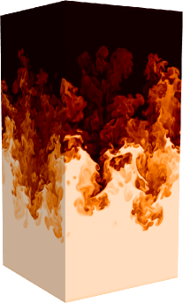
Figure 1: (a) Snapshot of temperature field for Rayleigh-Taylor turbulence at $t/\tau=2.6$. White (black) regions correspond to hot (cold) fluid. (b) Mean temperature profiles $\langle T(z)\rangle$ for times $t/\tau=1.4$ (continuous), $t/\tau=2.0$ (dashed) and $t/\tau=2.6$ (dotted). (c) Growth of the mixing layer thickness $h(t)$ defined as the vertical range for which $|\langle T(z)\rangle|\leq 0.98\theta_{0}/2$ compensated with the dimensional prediction $Agt^{2}$ in order to get the dimensionless coefficient $\alpha$. Filled symbols: $\alpha=h/(Agt^{2})$, open symbols: $\alpha=\dot{h}^{2}/(4Agh)$ Cabot and Cook (2006).

At time $t=0$ the system is at rest with cooler (heavier) fluid placed above the hotter (lighter) one. This corresponds to ${\bf v}({\bf x},0)=0$ and to a step function for the initial temperature profile: $T({\bf x},0)=-(\theta_{0}/2)\mbox{sgn}(z)$ where $\theta_{0}$ is the initial temperature jump which fixes the Atwood number $A=(1/2)\beta\theta_{0}$. The development of the instability leads to a mixing zone of width $h$ which starts from the plane $z=0$ and is dimensionally expected to grow in time according to $h(t)=\alpha Agt^{2}$ Dimonte and et al. (2004); Cabot and Cook (2006). Inside this mixing zone, turbulence develops in space and time. The phenomenological theory Chertkov (2003) predicts for velocity and temperature fluctuations the scaling laws

$$\delta_{r}v(t) \simeq (Ag)^{2/3}t^{1/3}r^{1/3}$$ (3)

$$\delta_{r}T(t) \simeq \theta_{0}(Ag)^{-1/3}t^{-2/3}r^{1/3}$$ (4)

The first relation represents Kolmogorov scaling with a time dependent energy flux $\epsilon\simeq(Ag)^{2}t$. ¿From the above scaling laws one obtains that the buoyancy term $\beta gT$ becomes subleading at small scales in (1), consistently with the assumption of passive transport of temperature fluctuations.

We integrate equations (1-2) by a standard $2/3$-dealiased pseudospectral method on a periodic domain with uniform grid spacing, square basis $L_{x}=L_{y}$ and aspect ratio $L_{x}/L_{z}=r$ with a resolution up to $512\times 512\times 2048$ ($r=1/4$). Time evolution is obtained by a second-order Runge-Kutta scheme with explicit linear part. In all runs, $Ag=0.25$, $Pr=\nu/\kappa=1$, $\theta_{0}=1$. Viscosity is sufficiently large to resolve small scales ($k_{max}\eta\simeq 1.2$ at final time). In the results, scales and times are made dimensionless with the box scale $L_{z}$ and the characteristic time $\tau=(L_{z}/Ag)^{1/2}$ Dalziel et al. (1999).

Rayleigh-Taylor instability is seeded by perturbing the initial condition with respect to the step profile. Two different perturbations were implemented in order to check the independence of the turbulent state from initial conditions. In the first case the interface $T=0$ is perturbed by a superposition of small amplitude waves in a narrow range of wavenumber around the most unstable linear mode Ramaprabhu et al. (2005). For the second set of simulations, we perturbed the initial condition by “diffusing” the interface around $z=0$. Specifically, we added a $10\%$ of white noise to the value of $T({\bf x},0)$ in a small layer of width $h_{0}$ around $z=0$.

Figure 1 shows a snapshot of the temperature field for a simulation with $r=1/2$ at advanced time. Large scale structures (plumes) identify the direction of gravity and break the isotropy. Nonetheless, we find that at small scales isotropy is almost completely recovered: the ratio of vertical to horizontal rms velocity is $v_{z}/v_{x}\simeq 1.8$ while for the gradients we have $\partial_{z}v_{z}/\partial_{x}v_{x}\simeq 1.0$. The horizontally averaged temperature $\langle T(z)\rangle$ follows closely a linear profile within the mixing layer where, therefore, the system recovers statistical homogeneity.

The analysis of the mixing layer width growth is also presented in Fig. 1. As shown by previous studies Ristorcelli and Clark (2004); Cabot and Cook (2006), the naive compensation of $h(t)$ with $Agt^{2}$ does not give a precise estimation of the coefficient $\alpha$ because of the presence of subleading terms which decay slowly in time. We have therefore implemented the similarity method introduced in Cabot and Cook (2006) which gives an almost constant value of $\alpha\simeq 0.038$ for $t/\tau\geq 1.5$, consistent with previous studies Ristorcelli and Clark (2004); Dimonte and et al. (2004).

Figure 2: Two-dimensional kinetic energy spectrum ($\circ$) and temperature spectrum ($\triangle$) at time $t/\tau=2.6$ corresponding to $R_{\lambda}=245$. Spectra are computed by Fourier transforming velocity and temperature fields on two-dimensional horizontal planes and averaging over $z$ in the mixing layer. Dashed lines represent Kolmogorov scaling $k^{-5/3}$. Lower inset: evolution in time of the amplitude of kinetic energy ($\times$) and temperature ($+$) spectra at fixed wavenumber $k_{0}=12$. Lines represent the dimensional predictions $t^{2/3}$ (continuous) and $t^{-4/3}$ (dashed) given by (3) and (4). Upper inset: inertial (continuous) and buoyancy (dashed) contributions to kinetic energy flux $\Pi(k)$ in Fourier space.

Figure 2 shows the kinetic energy $E(k)$ and temperature $E_{T}(k)$ spectra within the similarity regime. ¿From (3) and (4), we expect the following spatial-temporal scaling of spectra: $E(k,t)\sim t^{2/3}k^{-5/3}$ and $E_{T}(k,t)\sim t^{-4/3}k^{-5/3}$. Kolmogorov scaling $k^{-5/3}$ is evident for both velocity and temperature fluctuations. Moreover, self-similar temporal evolution of spectra is well reproduced, as shown in the lower inset. Also in Fig. 2 the two contributions to kinetic energy flux in spectral space are shown. Buoyancy contribution, dominant at large scale, becomes subleading at smaller scales, in agreement with the Kolmogorov-Obukhov picture. The above results, together with previous simulations Cabot and Cook (2006); Vladimirova and Chertkov (2008) and theoretical arguments Chertkov (2003), give a coherent picture of RT turbulence as a Kolmogorov cascade of kinetic energy forced by large scale temperature instability.

In the following we push this analogy one step ahead by showing that small scale fluctuations in RT turbulence display intermittency corrections typical of usual Navier–Stokes (NS) turbulence. Intermittency in turbulence is a consequence of non-uniform transfer of energy in the cascade which breaks down scale invariance. As a consequence, scaling exponents deviates from mean field theory and cannot be determined by dimensional arguments Frisch (1995). Several studies have been devoted to the intermittent statistics in NS turbulence, where the main issue concerns the possible universality of anomalous scaling exponent with respect to the forcing mechanisms and the large scale geometry of the flow. While universality has been demonstrated for the simpler problem of passive scalar transport, it is still an open issue for nonlinear NS turbulence. Therefore the key question is whether small scale statistics in RT turbulence is equivalent to the statistics observed in homogeneous, isotropic turbulence.

The simplest, and historically first, evidence of intermittency is in the dependence of energy dissipation on Reynolds number Champagne (1978); Atta and Antonia (1980); Meneveau and Sreenivasan (1987). Classical statistical indicators are the flatness $K$ of velocity derivatives Atta and Antonia (1980); Meneveau and Sreenivasan (1987) (corresponding to $K\simeq\langle\epsilon^{2}\rangle/\langle\epsilon\rangle^{2}$ in terms of energy dissipation), and the variance of the logarithm of kinetic energy dissipation which is expected to grow with Reynolds number as

$$\sigma_{\ln\epsilon}=a+(3\mu/2)\ln R_{\lambda}$$ (5)

The exponent $\mu$ is the key ingredient for the log-normal model of intermittency and its value is determined experimentally Atta and Antonia (1980); Sreenivasan and Kailasnath (1993) and numerically Yeung et al. (2006) to be $\mu\simeq 0.25$. More in general, moments of local energy dissipation are expected to have a power-law dependence on $R_{\lambda}$

$$\langle\epsilon^{p}\rangle\simeq\langle\epsilon\rangle^{p}R_{\lambda}^{\tau_{p}}$$ (6)

where the set of exponents $\tau_{p}$ can be predicted within the multifractal model of turbulence Frisch (1995); Boffetta and Romano (2002); Boffetta et al. (2008) in terms of the set of fractal dimensions $D(h)$.

Figure 3: Scaling of the variance of $\ln\epsilon$ on Reynolds number defined as $R_{\lambda}=(v_{z})_{rms}(\partial_{z}v_{z})_{rms}/\nu$, obtained from two realizations with white noise initial perturbation. The line is the best fit corresponding to $\mu=0.24$ in (5). Inset: scaling exponents of the moments of local dissipation $\tau_{p}$ obtained from best fits according to (6). The line represents the log-normal approximation $\tau_{p}=(3/4)\mu(p^{2}-p)$.

Because in RT turbulence the Reynolds number increases in time, it provides a natural framework for a check of (5) and (6). Figure 3 shows the dependence of the variance of $\ln\epsilon$ on $R_{\lambda}$ together with the first moments of energy dissipation. Despite the limited range of $R_{\lambda}$, a clear scaling of $\ln\epsilon$ is observable, even if with some fluctuations. The best fit with (5) gives an exponent $\mu\simeq 0.24$, very close to what observed in homogeneous, isotropic turbulence Yeung et al. (2006).

Scaling exponents $\tau_{p}$ for the moments of dissipation (6) are also shown in Fig. 3. We were able to compute moments up to $p=2$ with statistical significance. Log-normal approximation, which is in general valid for $p\to 0$, is found to be unsatisfactory for larger values of $p$. For $p=2$, which corresponds to the flatness $K$ of velocity derivatives, we find $\tau_{2}\simeq 0.27$. This result is consistent with experiments at comparable Reynolds numbers Atta and Antonia (1980) which shows that $K\sim R_{\lambda}^{0.2}$ for $R_{\lambda}<200$ while an asymptotic exponent $\tau_{2}\simeq 0.41$ is reached for $R_{\lambda}>10^{3}$ only.

Figure 4: Scaling exponents of isotropic longitudinal velocity structure functions $S_{p}(r)=\langle\left(\delta_{r}{\bf v}\cdot\hat{\bf r}\right)^{p}\rangle$ ($\hat{\bf r}={\bf r}/r$) for the late stage of RT turbulence (open circle). Exponents are computed by compensation of $S_{p}(r)$ with $S_{3}(r)$, according to the ESS procedure Benzi et al. (1993) averaging inside the mixing layer and on all directions. Filled circles: scaling exponents from simulations of homogeneous, isotropic turbulence at $R_{\lambda}=381$ Gotoh et al. (2002). Line represents dimensional prediction $\zeta_{p}=p/3$. Inset: third-order isotropic longitudinal structure function $S_{3}(r)$. The line represents Kolmogorov’s four-fifth law $S_{3}(r)=-4/5\epsilon r$.

In NS turbulence intermittency is also observed in the inertial range of scales as deviations of velocity structure functions $S_{p}(r)=\langle(\delta_{r}v)^{p}\rangle$ from the dimensional prediction (3) which corresponds to $S_{p}(r)\simeq r^{p/3}$ Frisch (1995). Anomalous scaling is observed, which corresponds to scaling laws $S_{p}(r)\simeq r^{\zeta_{p}}$ with a set of exponents $\zeta_{p}\neq p/3$. We remind that constancy of energy flux in the inertial range implies $\zeta_{3}=1$ independently on intermittency, as required by the Kolmogorov’s “four-fifths” law $S_{3}(r)=-4/5\epsilon r$ Frisch (1995), which is indeed observed in our simulations (see inset of Fig. 4). Figure 4 shows the first longitudinal scaling exponents computed from our simulations exploiting the extended self-similarity procedure which allows for a precise determination of the exponents at moderate Reynolds numbers Benzi et al. (1993). A deviation from dimensional prediction $\zeta_{p}=p/3$ is clearly observable for higher moments. Fig. 4 also shows the scaling exponents obtained from a homogeneous, isotropic simulation of NS equations at a comparable $R_{\lambda}$ Gotoh et al. (2002). The two sets agree within the error bars, this gives further quantitative evidence in favor of the equivalence between RT turbulence and NS turbulence in three dimensions.

We end by discussing the behavior of turbulent heat flux and rms velocity fluctuations as a function of the mean temperature gradient. In terms of dimensionless variables, these quantities are represented respectively by the Nusselt number $Nu=1+\langle v_{z}T\rangle L/(\kappa\theta_{0})$, the Reynolds numbers $Re=v_{rms}L/\nu$ and Rayleigh number $Ra=AgL^{3}/(\nu\kappa)$. The relations between these quantities has been object of many experimental and numerical studies in past years, mainly in the context of Rayleigh-B$\acute{e}$nard turbulent convection Siggia (1994); Grossmann and Lohse (2000); Niemela et al. (2000); Nikolaenko and Ahlers (2003); Lohse and Toschi (2003); Celani et al. (2006). Experiments have reported both simple scaling laws $Nu\sim Ra^{\beta}$ with exponent $\beta$ scattered around $\beta=0.3$ Glazier et al. (1999); Niemela et al. (2000) and, more complicated behavior Xu et al. (2000); Nikolaenko and Ahlers (2003) partially in agreement with a phenomenological theory Grossmann and Lohse (2000). However, in the limit of very large $Ra$, Kraichnan Kraichnan (1962) predicted an asymptotic scaling $Nu\sim Ra^{1/2}$ now called the ultimate state of thermal convection. This regime is expected to hold when thermal and kinetic boundary layers become irrelevant, and indeed has been observed in numerical simulation of thermal convection at moderate $Ra$ when boundaries are artificially removed Lohse and Toschi (2003). It is therefore natural to expect that the ultimate state scaling arises in RT convection where boundaries are absent.

The ultimate state relations can formally be obtained from kinetic energy and temperature balance equations Grossmann and Lohse (2000). In the context of RT turbulence, they are a simple consequence of the dimensional scaling of the mixing length $L\equiv h\simeq Agt^{2}$ and of the rms velocity $v_{rms}\simeq Agt$. Inserting in the definition of the dimensionless numbers one obtains

$$Nu\sim Pr^{1/2}Ra^{1/2}\,,\mbox{\hskip 28.45274pt}Re\sim Pr^{-1/2}Ra^{1/2}$$ (7)

where $Pr=\nu/\kappa$.

Figure 5: The scaling of Nusselt number (open circles) and Reynolds number (solid circles) as functions of Rayleigh number. Lines represent the ultimate state predictions (7).

We remark that the above relations are independent on the statistics of the inertial range and on the presence of intermittency as they involve large scale quantities only. Our numerical results, shown in Fig. 5, confirms the ultimate state scaling (7). The same behavior has been predicted and observed for two-dimensional RT simulations, where temperature fluctuations are not passive and Bolgiano scaling is observed in the inertial range Celani et al. (2006). The elusive Kraichnan scaling in thermal convection finds its natural manifestation in Rayleigh-Taylor turbulence, which turns out to be an excellent setup for experimental studies in this direction.

References

- Schultz and et al. (2006) D. Schultz and et al., J. Atmos. Sci. 10, 1409 (2006).
- Zingale et al. (2005) M. Zingale, S. Woosley, C. Rendleman, M. Day, and J. Bell, Astrophys. J. 632, 1021 (2005).
- Cabot and Cook (2006) W. Cabot and A. Cook, Nature Physics 2, 562 (2006).
- Isobe et al. (2005) H. Isobe, T. Miyagoshi, K. Shibata, and T. Yokoyama, Nature 434, 478 (2005).
- Fujioka and et al. (2004) S. Fujioka and et al., Phys. Rev. Lett. 92, 195001 (2004).
- Chertkov (2003) M. Chertkov, Phys. Rev. Lett. 91, 115001 (2003).
- Vladimirova and Chertkov (2008) N. Vladimirova and M. Chertkov, Arxiv preprint arXiv:0801.2981 (2008).
- Poujade (2006) O. Poujade, Phys. Rev. Lett. 97, 185002 (pages 4) (2006).
- Dimonte and et al. (2004) G. Dimonte and et al., Phys. Fluids 16, 1668 (2004).
- Dalziel et al. (1999) S. Dalziel, P. Linden, and D. Youngs, J. Fluid Mech. 399, 1 (1999).
- Ramaprabhu et al. (2005) P. Ramaprabhu, G. Dimonte, and M. Andrews, J. Fluid Mech. 536, 285 (2005).
- Ristorcelli and Clark (2004) J. Ristorcelli and T. Clark, J. Fluid Mech. 507, 213 (2004).
- Frisch (1995) U. Frisch, Turbulence: The Legacy of AN Kolmogorov (Cambridge University Press, 1995).
- Champagne (1978) F. Champagne, Journal of Fluid Mechanics 86, 67 (1978).
- Atta and Antonia (1980) C. V. Atta and R. Antonia, Phys. Fluids 23, 252 (1980).
- Meneveau and Sreenivasan (1987) C. Meneveau and K. Sreenivasan, Phys. Rev. Lett. 59, 1424 (1987).
- Sreenivasan and Kailasnath (1993) K. Sreenivasan and P. Kailasnath, Phys. Fluids A 5, 512 (1993).
- Yeung et al. (2006) P. Yeung, S. Pope, A. Lamorgese, and D. Donzis, Phys. Fluids 18, 065103 (2006).
- Boffetta and Romano (2002) G. Boffetta and G. Romano, Phys. Fluids 14, 3453 (2002).
- Boffetta et al. (2008) G. Boffetta, A. Mazzino, and A. Vulpiani, J. Phys. A 41, 363001 (2008).
- Benzi et al. (1993) R. Benzi, S. Ciliberto, R. Tripiccione, C. Baudet, F. Massaioli, and S. Succi, Phys. Rev. E 48, R29 (1993).
- Gotoh et al. (2002) T. Gotoh, D. Fukayama, and T. Nakano, Phys. Fluids 14, 1065 (2002).
- Siggia (1994) E. Siggia, Ann. Rev. Fluid Mech. 26, 137 (1994).
- Grossmann and Lohse (2000) S. Grossmann and D. Lohse, J. Fluid Mech. 407, 27 (2000).
- Niemela et al. (2000) J. Niemela, L. Skrbek, K. Sreenivasan, and R. Donnelly, Nature 404, 837 (2000).
- Nikolaenko and Ahlers (2003) A. Nikolaenko and G. Ahlers, Phys. Rev. Lett. 91, 084501 (2003).
- Lohse and Toschi (2003) D. Lohse and F. Toschi, Phys. Rev. Lett. 90, 034502 (2003).
- Celani et al. (2006) A. Celani, A. Mazzino, and L. Vozella, Phys. Rev. Lett. 96, 134504 (2006).
- Glazier et al. (1999) J. Glazier, T. Segawa, A. Naert, and M. Sano, Nature 398, 307 (1999).
- Xu et al. (2000) X. Xu, K. Bajaj, and G. Ahlers, Phys. Rev. Lett. 84, 4357 (2000).
- Kraichnan (1962) R. Kraichnan, Phys. Fluids 5, 1374 (1962).