Possibility of Coherent Phenomena like Bloch Oscillations with Single Photons via $W$-States

Abstract

We examine the behavior of single photons at multiport devices and enquire if coherent effects are possible. In particular we study how single photons need to be manipulated in order to study coherent phenomena. We show that single photons need to be produced in W-states which lead to vanishing mean amplitude but nonzero correlations between the inputs at different ports. Such correlations restore coherent effects with single photons. As a specific example we demonstrate Bloch oscillations with single photons and thus provide strict analog of Bloch oscillation of electrons.

I Introduction

Experiments with single photons have been at the heart of Quantum optics. About a century ago Taylor enquired if it is possible to do Young’s double slit experiment with a feeble source of photons Taylor . His answer was yes provided the experiment was done for long enough which was about $2000$ hours in his case. The interest in single photon interference experiments has been revived as now we have the possibility of heralded single photon source Alfred ; Fasel ; Pittman ; Bertocchi ; Zavatta ; Shi . Variety of other possibilities with single photon sources have been discussed Mandel . These for example include interaction free measurements Elitzur ; Kwiat , Wheeler’s delayed choice measurements Hellmuth ; Jacques and delayed choice quantum eraser Kim . Application of single photons in quantum imaging Sergienko ; Teich ; Howell ; Rubin have been discussed and single photons are finding increasing use in quantum information science Walmsley ; Brien . Linear optical elements like beam splitters; waveguides; phase shifters; polarization beam splitter have been studied to process information with single photons Hong ; Pathak ; Politi ; Nagata . The behavior of such elements is quite different for single photons and for weak coherent light. The interpretation of single photon interference experiments is always intriguing Feynman ; Dirac . For example the interference with single photons in a Mach-Zehnder interferometer can be understood in terms of the non-factorizability of the quantum states of the two mode into which a single mode of light is split by the action of the beam splitter. Motivated by the above we enquire generally whether coherent phenomena can be possible with incoherent single photon sources. We show that one needs to make a $W$-state Dur ; Eibl out of a single photon source. This is possible by the use of a multiport beam splitter. The $W$-state has strong quantum correlations even though it has no coherent component for the field amplitudes. The quantum correlations in the $W$-state are responsible for restoring the coherent effects.

The organization of the paper is as follows : In section II, we show coherent effects can be possible with incoherent single photon sources. In section III, we demonstrate the possibility of coherent Bloch oscillations Bloch ; Peschel ; Pertsch using single photon sources. This fills a gap that has existed as Bloch oscillations with coherent light fields do not provide strict analog of the Bloch oscillations for the case of electrons. In the latter case we have a quantum particle whereas in the case of coherent beam of light we have a classical source. We summarize our results in section IV and conclude with future perspectives.

II Possibility of coherent Phenomena using Incoherent single Photon $W$-States

In order to understand the role of coherence and correlations, consider interference of the two beams of light. Let each beam be characterized by the annihilation and creation operators $a_{\alpha}$ and ${a_{\alpha}}^{\dagger}$; $\alpha$= $1$, $2$. We write the total field operator after the two beams are made to interfere as

$$b_{1} = ({a_{1}+e^{i\theta}a_{2}})/{\sqrt{2}}~{}.$$ (1)

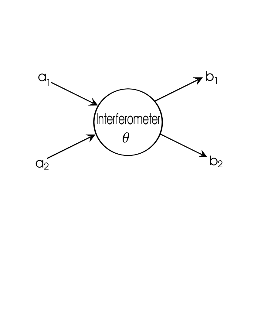
Figure 1: Schematic diagram of a two beam interferometer.

The mean intensity of the output $b_{1}$ is then

$$\langle{b_{1}}^{\dagger}b_{1}^{\vphantom{\dagger}}\rangle = \frac{\langle a_{1}^{\dagger}a_{1}^{\vphantom{\dagger}}\rangle+\langle a_{2}^{\dagger}a_{2}^{\vphantom{\dagger}}\rangle+e^{i\theta}\langle a_{1}^{\dagger}a_{2}\rangle+e^{-i\theta}\langle a_{2}^{\dagger}a_{1}\rangle}{2}~{}.$$

Clearly for interference to occur we need

$$\langle{a_{1}}^{\dagger}a_{2}^{\vphantom{\dagger}}\rangle \neq 0~{}.$$ (3)

If the two beams are in coherent states, then

$$\langle{a_{1}}^{\dagger}a_{2}^{\vphantom{\dagger}}\rangle = \langle{a_{1}}^{\dagger}\rangle\langle a_{2}^{\vphantom{\dagger}}\rangle~{},$$ (4)

and thus interference obviously occurs. If on the other hand the input state were Fock state $|n_{1},n_{2}\rangle$, then $\langle{a_{1}}^{\dagger}a_{2}^{\vphantom{\dagger}}\rangle=0$ and no interference occurs in the mean intensity given by (2). We are required to have non-zero correlation $(3)$. Thus one can consider an entangled state of the form

$$|\psi\rangle = \frac{(|1,0\rangle+|0,1\rangle)}{\sqrt{2}}~{},$$ (5)

then

$$\langle{a_{1}}^{\dagger}a_{2}^{\vphantom{\dagger}}\rangle = \frac{1}{2}~{}.$$ (6)

Therefore for the observation of interference at the level of mean intensity one needs to have non-zero correlation which is possible with a state like $(5)$ unless one is dealing with coherent beams of light.

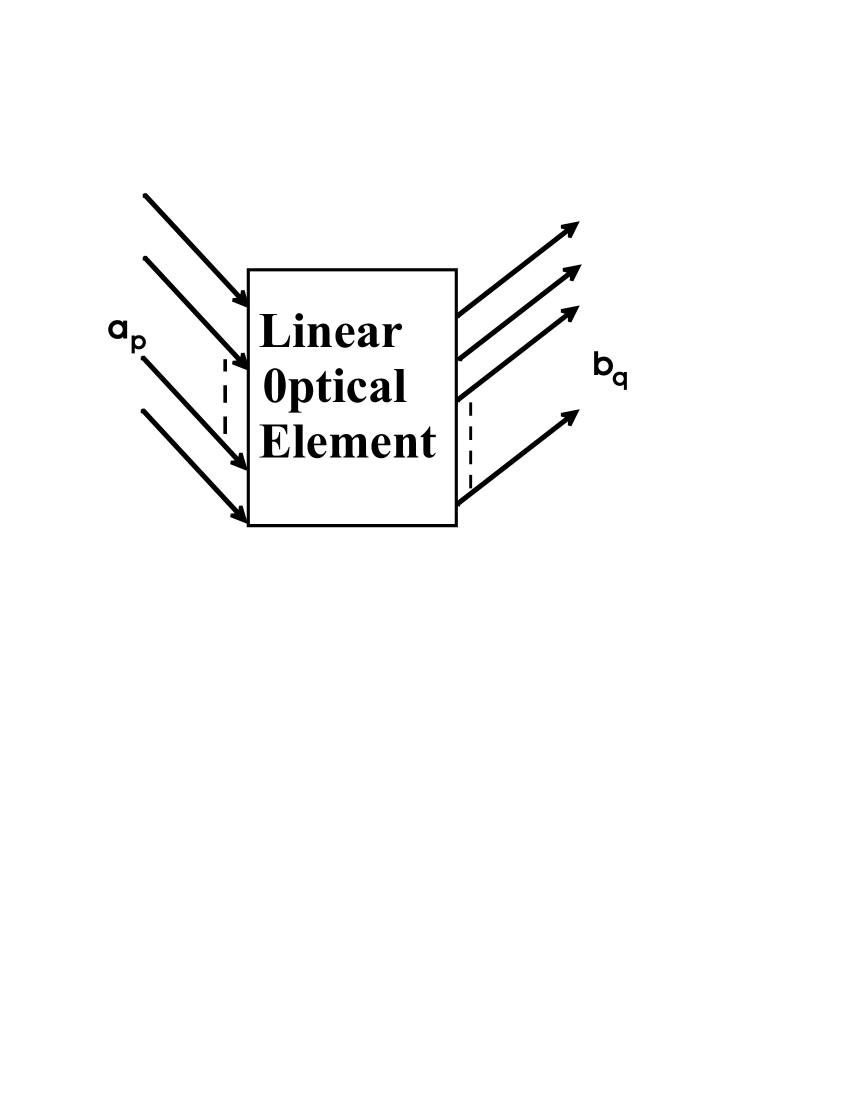
Figure 2: The figure shows the linear optical element with input fields $a_{p}$ (for $p$=1, . . . ,N) and output fields $b_{q}$.

Let us consider a more general situation with several inputs and several outputs for an optical element. We write the input-output relation as

$$b_{q} = \sum_{p=1}^{N}G_{p,\hskip 0.56917ptq}\hskip 0.85355pta_{p}~{},$$ (7)

where $G$ depends on the linear optical element and is equal to $\delta_{p\hskip 0.56917ptq}$ in the absence of the optical element. If all the inputs are in coherent states with amplitudes $\alpha_{p}$, then

$$\langle b_{q}^{\vphantom{\dagger}}\rangle = \sum G_{p,\hskip 0.56917ptq}\hskip 0.85355pt\alpha_{p}~{},$$ (8)

and

$$\langle b_{q}^{\dagger}b_{q}^{\vphantom{\dagger}}\rangle = |\langle b_{q}^{\vphantom{\dagger}}\rangle|^{2}\equiv\Big{|}\sum_{p}G_{p,\hskip 0.56917ptq}\hskip 0.85355pt\alpha_{p}\Big{|}^{2}~{}.$$ (9)

On the other hand if the inputs are incoherent, then we loose all coherent effects

$$\langle b_{q}^{\dagger}b_{q}^{\vphantom{\dagger}}\rangle\equiv\sum_{p}{G}_{p,\hskip 0.28436ptq}^{*}G_{p,\hskip 0.56917ptq}\hskip 0.85355pt\langle{a_{p}}^{\dagger}a_{p}^{\vphantom{\dagger}}\rangle~{}.$$ (10)

The question is$-$ how can one restore the interference effects with single photons. In order to see what is needed to restore the interference effects we use (7) and write the output intensity in the form

$$\langle b_{q}^{\dagger}b_{q}^{\vphantom{\dagger}}\rangle\equiv\sum_{r,\hskip 0.56917pts}{G}_{q,\hskip 0.28436ptr}^{*}G_{q,\hskip 0.56917pts}\hskip 0.85355pt\langle{a_{r}}^{\dagger}a_{s}^{\vphantom{\dagger}}\rangle~{}.$$ (11)

Therefore for ensuring the interference effects of the type implied by (9), we need to have

$$\langle{a_{r}}^{\dagger}a_{s}^{\vphantom{\dagger}}\rangle \neq 0\hskip 5.69046pt\forall\hskip 2.84544ptr,s$$ (12)

even if $\langle a_{r}^{\vphantom{\dagger}}\rangle=0$. One may be able to find several states satisfying (12) we have found that if the input fields are in a $W$ state, then (12) holds. Let us represent the input single photon state as a $W$ state

$$|\psi\rangle\equiv\sum_{p=1}^{N}c_{p}|1_{p},\{0\}\rangle,$$

$$\sum_{p}|c_{p}|^{2}=1~{},$$ (13)

and where $|1_{p},\{0\}\rangle$ denotes single photon at the $p^{th}$ input and no photons at the remaining inputs. Traditionally one takes $c_{p}=1/\sqrt{N}$ but it is not essential. The $W$-state has the unusual property

$$\langle a_{p}^{\dagger}a_{q}^{\vphantom{\dagger}}\rangle=c_{p\hskip 0.56917pt}\hskip 0.28436pt^{*}c_{q}\hskip 0.85355pt,\langle a_{p}\rangle=0~{};$$ (14)

and hence the output (in Eq. (11)) becomes

$$\langle b_{q}^{\dagger}b_{q}^{\vphantom{\dagger}}\rangle=\Big{|}\sum_{p}G_{p,\hskip 0.56917ptq}\hskip 0.85355ptc_{p}\Big{|}^{2}~{}.$$ (15)

Thus the $W$-state for a single photon behaves like a coherent input for observations of interference at the level of mean intensity. We have thus proved that any $W$-state of the form (13) would exhibit interference phenomena like that exhibited by a coherent state if the amplitude of the coherent state is substituted for the quantum amplitudes in the superposition (13).

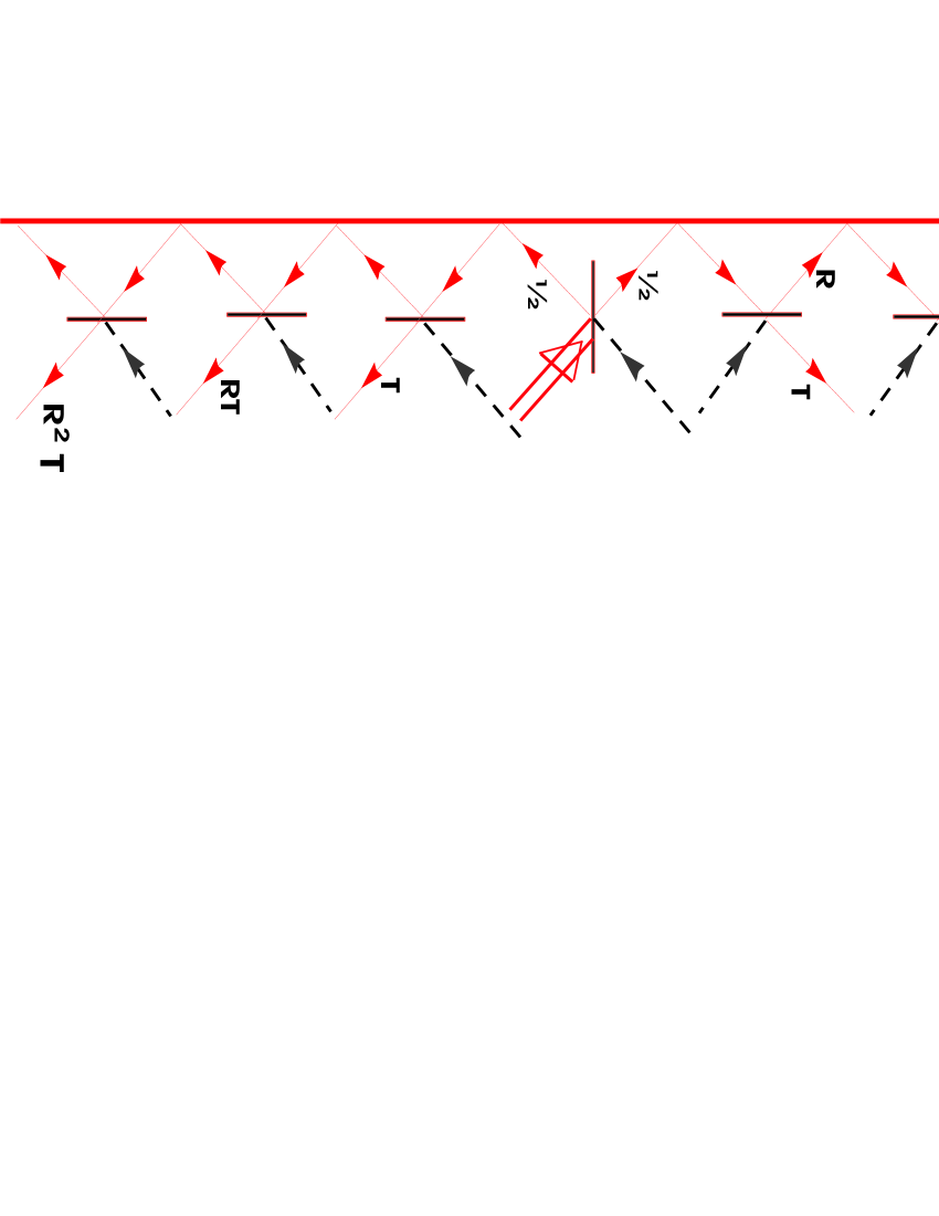
Figure 3: (Color online) Figure shows the scheme for generating the required input $W$-state. The thick red line is the mirror with $100\%$ reflectivity. The double arrow indicates a heralded single photon from a source like parametric downconverter. All black lines show vacuum fields at open ports. The transmissivity of the beam splitter is $T$. The output intensities at different ports are given by $---TR^{2}/2,TR/2,T/2,T/2,TR/2,TR^{2}/2---$.

We next discuss the arrangement that can produce the $W$-state (13). In the Fig. 3 we show how using a multiport optical splitter Zukowski ; Paternostro one can produce single photon $W$-state starting from a heralded single photon source which has been used by many workers. We show in the Fig. 4 the distribution of $|c_{p}|$ produced by the arrangement of the Fig. 3. In the next section we present an illustrative example of the use of the $W$-state in producing coherent effects.

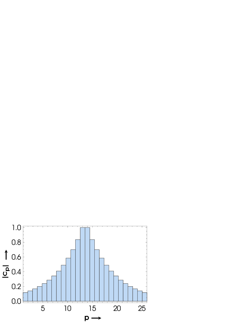
Figure 4: (Color online) Figure shows distribution of $|c_{p}|$ as a function of $p$.

III Coherent Bloch Oscillations using Single Photon $W$-states as input to Coupled Waveguides

The demonstration of Bloch oscillations using optical elements has attracted considerable attention. It turned out that such a coherent phenomena which was first discussed in the context of motion of electrons Bloch in a periodic potential and an electric field can be demonstrated using simple optical structures and coherent light beams Pertsch ; Peschel . In view of the current interest in single photon states it is natural to explore the possibility of Bloch oscillations with single photons. This would be strict quantum analog of electronic Bloch oscillations. On the basis of our discussion in Sec II, we show that Bloch oscillations with single photons are indeed possible provided we prepare single photons in a $W$-state.

We consider an array of $N$ evanescently coupled single-mode waveguides hagai ; Z , with a linearly varying refractive index across the array. The mode for the field in the $p^{th}$ waveguide is described by the annihilation operator $a_{p}(t)$. These obey Bosonic commutation relations. The Hamiltonian in terms of the Heisenberg operators can be written in the form

$$H=\hbar\sum_{p}\delta\hskip 0.85355ptp\hskip 0.85355pta_{p}^{\dagger}\hskip 1.42271pta_{p}^{\vphantom{\dagger}}+\hbar\sum_{p}J(a_{p}^{\dagger}\hskip 1.42271pta_{p+1}^{\vphantom{\dagger}}+a_{p+1}^{\dagger}\hskip 1.42271pta_{p}^{\vphantom{\dagger}})~{},$$ (16)

where $J$ is the coupling between the nearest neighbor waveguides and the sum is over nearest neighbors. The refractive index of $p^{th}$ waveguide depends on the index $p$ of the waveguide. Note that in the electron problem the first term in $(16)$ corresponds to the electric field and the second term to the periodic potential. The Heisenberg equations of motion are

$$\dot{a}_{p}=-i\delta\hskip 0.85355ptp\hskip 1.42271pta_{p}^{\vphantom{\dagger}}-iJ(\hskip 1.42271pta_{p+1}^{\vphantom{\dagger}}+a_{p-1})~{},$$ (17)

Because of the linearity of the equations (17); the Heisenberg operators at time $t$ can be expressed in terms of the operators at time $t=0$

$$a_{p}(t) = \sum_{q}G_{p,\hskip 0.56917ptq}\hskip 0.85355pt(t)a_{q}(0)~{},$$ (18)

where

$$\dot{G}_{p,\hskip 0.56917ptq}\hskip 0.28436pt(t)=-i\delta\hskip 0.85355ptp\hskip 1.42271ptG_{p,\hskip 0.56917ptq}^{\vphantom{\dagger}}-iJ(\hskip 1.42271ptG_{p+1,q}^{\vphantom{\dagger}}+G_{p-1,q})~{},$$ (19)

and where the initial condition is

$$G_{p,\hskip 0.28436ptq}\hskip 0.85355pt(0)=\delta_{pq}~{}.$$ (20)

It should be borne in mind that the parameter $t$ is related to the propagation distance by $t=zn/c$ where $n$ is the refractive index for the mode of the waveguide. For large number of waveguides, the Eq. (19) can be solved in terms of Bessel functions. The method of solution is similar to the one in Ref. Peschel and is based on the use of Fourier series representation. The result can be written as footnote1

$$G_{p,\hskip 0.28436ptq}\hskip 0.56917pt(t)=\exp\Big{[}i\alpha q\tau+\frac{i(p-q)\hskip 0.56917pt(\alpha\tau-\pi)}{2}\Big{]}J_{q-p}[\frac{4}{\alpha}\sin(\frac{\alpha\tau}{2})],\hskip 0.56917pt\tau\equiv Jt,\alpha=\delta/J~{}.$$

We can calculate the output for different initial states of single photon. Consider an arrangement of $2\hskip 0.56917ptN$ waveguides. Let single photon be launched in the ${N}^{th}$ waveguide. Then the output distribution is given by

$$I_{p} = \langle a_{p}^{\dagger}(t)a_{p}(t)^{\vphantom{\dagger}}\rangle$$ (22)

$$= \Big{|}G_{p,\hskip 0.28436ptN}(t)\hskip 0.85355pt\Big{|}^{2}$$

$$= \Big{|}J_{p-N}[\frac{4}{\alpha}\sin(\frac{\alpha\tau}{2})]\Big{|}^{2}~{}.$$

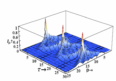
Figure 5: (Color online) Figure shows the variation of output intensity distribution $I_{p}$ for a single waveguide excitation as a function of $\tau$ for $p$=1, . . . ,26. The parameter $\alpha$ is $\alpha=0.5$.

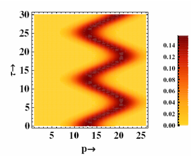
Figure 6: (Color online) Figure shows the Bloch oscillation for a Gaussian excitation. The number of waveguides in the system is $26$ and the parameter for the Gaussian beam are chosen as $\sigma=3.6$, and $\bar{p}=13$. The parameter $\alpha$ is $\alpha=0.5$.

This is shown in the Fig. 5. The behavior is determined by the zeroes of the Bessel function.

Next we consider the well known coherent Bloch oscillation when the input to each waveguide is in a coherent state with amplitude $\alpha_{p}$. In order to exhibit Bloch oscillations one needs fairly wide distribution of fields at different inputs. We assume as in the work of Peschel et al. Peschel , a Gaussian distribution of $\alpha_{p}$ i.e. we assume $\alpha_{p}\sim\exp[-\hskip 0.56917pt{{(p-\bar{p})}^{2}}/{2\hskip 1.42271pt\sigma^{2}}]$ upto a constant. The resulting Bloch oscillation is shown in the Fig. 6.

Next we show how the quantum correlations in a $W$-state enable us to obtain coherent Bloch oscillations with single photons. For this purpose we assume that the input to the waveguides is from the multiport device of the Fig. 3. The state of the field at the input would be given by Eq (13) with a distribution of $c_{p}$’$s$ given by the Fig. 4. The amplitudes $c_{p}$’$s$ would in principle have complex phase factors associated with the propagation distance from the beam splitter BS to the $100$% mirror and back. These factors have been set as unity. For single photon in a $W$-state we get

$$I_{p}=\Big{|}\sum_{q}G_{p,\hskip 0.56917ptq}(t)\hskip 0.85355ptc_{q}\Big{|}^{2}~{},$$ (23)

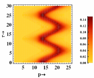
Figure 7: (Color online) Figure shows the Bloch oscillation for a $W$-state. The parameter $\alpha$ is chosen as $\alpha=0.5$ and the number of waveguides in the system is 26.

where we use $c_{q}$’$s$ from the Fig. 4. This distribution of the intensity is shown in the Fig. 7. In this case we recover the coherent Bloch oscillations even though we use incoherent single photons. This is possible due to the quantum correlations implicit in the $W$-state of single photons. The similarity between Figs. 6 and 7 is striking. This is because of the similarity of the results (9) and (15). In order to produce the pattern in Fig. 6 with single photons we need an optical device which would produce a distribution of $c_{p}$’$s$ (in Eq. (13)) given by a Gaussian distribution.

An understanding of the Bloch oscillation resulting from (23) can be obtained by using Fourier space footnote35 . Let us write

$$c_{q}=\frac{1}{\sqrt{2\pi}}\int_{-\pi}^{\pi}\tilde{c}(k)\hskip 1.13791pte^{ikq}dk\hskip 0.85355pt~{},$$

$$\tilde{c}(k)=\frac{1}{\sqrt{2\pi}}\sum_{q}c_{q}\hskip 1.13791pte^{-ikq}$$ (24)

Then (23) can be written as

$$I_{p}=\frac{1}{2\pi}\Big{|}\int_{-\pi}^{\pi}\tilde{c}(k-\alpha\hskip 0.85355ptt)\hskip 0.85355pte^{ikp}\exp\Big{[}\frac{2i}{\alpha}[\sin(k)-\sin(k-\alpha\hskip 0.85355ptt)]\Big{]}dk\Big{|}^{2}~{},$$ (25)

Figure 8: Figure shows the distribution of $|\tilde{c}({k})|^{2}$ as a function of $k$.

This in fact was an intermediate step in the derivation of (21). For the $c_{q}$ given by the Fig. 4, the distribution $|\tilde{c}({k})|^{2}$ is shown in the Fig. 8. The distribution is centered at zero and has a width, at half height, $0.31$, which is quite small in comparison to the range of $k$ values [$-\pi$ to $\pi$]. Thus an estimate of the behavior of the integral in (25) can be obtained by expanding the exponential around $\alpha\hskip 0.85355ptt$ i.e. we set $k\sim(\alpha\hskip 0.85355ptt+\delta)$ and approximate

$$\exp\Big{[}\frac{2i}{\alpha}[\sin(k)-\sin(k-\alpha\hskip 0.85355ptt)]\Big{]}\approx\exp\Big{[}\frac{2i}{\alpha}\sin(\alpha\hskip 0.85355ptt)-\frac{4i}{\alpha}\hskip 0.85355pt\delta\sin^{2}(\frac{\alpha\hskip 0.85355ptt}{2})\Big{]}~{},$$ (26)

We have retained terms to lowest order in $\delta$. On substituting (26) in (25) we get

$$I_{p} \cong\frac{1}{2\pi}\Big{|}\int\tilde{c}(\delta)\hskip 0.85355pte^{i\hskip 1.13791pt\delta\hskip 0.85355pt(p-\frac{4}{\alpha}\sin^{2}(\frac{\alpha\hskip 0.85355ptt}{2}))}\exp\Big{[}i\hskip 0.85355ptp\hskip 0.85355pt{\alpha}\hskip 0.85355ptt+\frac{2\hskip 0.85355pti}{\alpha}\sin(\alpha\hskip 0.85355ptt)\Big{]}\hskip 0.85355ptd\delta\Big{|}^{2}~{},$$ (28)

$$\cong|c_{\bar{p}}|^{2},\hskip 0.85355pt\bar{p}\equiv{\Big{(}p-\frac{4}{\alpha}\sin^{2}(\frac{\alpha t}{2})\Big{)}}~{}.$$

The structure shown in the Fig. 7 is in conformity with the approximate formula (28). The revivals in the intensity distribution are related to the zeros of $\sin^{2}(\alpha\hskip 0.85355ptt/2)$.

Finally note that the observation of the single photon Bloch oscillation would require (a) heralded source of single photons of the type used in Refs. Bertocchi ; Zavatta ; Shi ; Politi (b) waveguide structures as for example the ones employed in Refs. hagai ; Z ; Politi ; iwanow (c) mirror assembly of the type discussed by Zukowski et al. Zukowski . Since all the relevant optical elements are currently in use, the observation of Bloch oscillations with single photons should be possible.

IV Conclusions

To conclude, we investigated generally how one can observe the coherent effects with incoherent single photon sources. For this purpose one has to convert single photon source into something with a spatial waveform. We used a multiport beam splitter to prepare single photon $W$-state. Note that recently one has demonstrated several other interesting possibilities to produce single photon sources with required waveforms Yarnall ; Kolchin . Further by using other types of multiport devices like the ones discussed in Ref Zukowski we can make the magnitudes of all $c_{p}$ same. As an application we consider the propagation of light in waveguide array and explored the possibility of observing Bloch oscillations with single photons. Our results show that the Bloch oscillations are possible with single photon $W$-state. The quantum correlations in the $W$-state are responsible for restoring the Bloch oscillations. There are number of other possibilities using $W$-state for single photons. For example a phase object in the path of one of the beams would change the coefficient $c_{p}$ to $c_{p}e^{i\phi_{p}}$ and thus the final interference pattern can be used to derive information on the object.

References

- (1) G. I. Taylor, Proc. Cambridge Philos. Soc. 15, 114115 (1909).
- (2) A. B. U’Ren, C. Silberhorn, K. Banaszek, and I. A. Walmsley, Phys. Rev. Lett. 93, 093601 (2004).
- (3) S. Fasel, O. Alibart, A. Beveratos, S. Tanzilli, H. Zbinden, P. Baldi, and N. Gisin, New J. of Phys. 6, 163 (2004).
- (4) T.B. Pittman, B.C. Jacobs, and J.D. Franson, Opt. Commun. 246, 545 (2005).
- (5) G. Bertocchi, O. Alibart, D. B. Ostrowsky, S. Tanzilli, and P. Baldi, J. Phys. B 39, 1011 (2006).
- (6) A. Zavatta, S. Viciani, and M. Bellini, Science 306, 660 (2004).
- (7) X. Shi, A. Valencia, M. Hendrych, and J. P. Torres, Opt. Lett. 33, 875 (2008).
- (8) L. Mandel, Rev. Mod. Phys. 71, S274 (1999).
- (9) A. Elitzur and L. Vaidman, Found. Phys. 23, 987 (1993).
- (10) P. Kwiat, H. Weinfurter, T. Herzog, A. Zeilinger, and M. A. Kasevich, Phys. Rev. Lett. 74, 4763 (1995).
- (11) T. Hellmuth, H. Walther, A. Zajonc, and W. Schleich, Phys. Rev. A 35, 2532 (1987).
- (12) V. Jacques, E. Wu, F. Grosshans, F. Treussart, P. Grangier, A. Aspect, and J. Roch, Science 315, 966 (2007).
- (13) Y. H. Kim, R. Yu, S. P. Kulik, Y. Shih, and M. O. Scully, Phys. Rev. Lett. 84, 1 (2000).
- (14) T. B. Pittman, Y. H. Shih, D. V. Strekalov, and A. V. Sergienko, Phys. Rev. A 52, R3429 (1995).
- (15) A. F. Abouraddy, P. R. Stone, A. V. Sergienko, B. E. A. Saleh, and M. C. Teich, Phys. Rev. Lett. 93, 213903 (2004).
- (16) R. S. Bennink, S. J. Bentley, R. W. Boyd, and J. C. Howell, Phys. Rev. Lett. 92, 033601 (2004).
- (17) M. H. Rubin and Y. Shih, Phys. Rev. A 78, 033836 (2008).
- (18) I. A. Walmsley and M. G. Raymer, Science 307, 1733 (2005).
- (19) J. L. O’Brien, Science 318, 1567 (2007).
- (20) C. K. Hong, Z. Y. Ou, and L. Mandel, Phys. Rev. Lett. 59, 2044 (1987).
- (21) P. K. Pathak and G. S. Agarwal, Phys. Rev. A 75, 032351 (2007).
- (22) A. Politi, M. J. Cryan, J. G. Rarity, S. Yu, and J. L. O’Brien, Science 320, 646 (2008).
- (23) T. Nagata, R. Okamoto, J. L. O’Brien, K. Sasaki, and S. Takeuchi , Science 316, 726 (2007).
- (24) R. P. Feynman, R. B. Leighton, and M. L. Sands, The Feynman Lectures on Physics (Addison-Wesley, Reading, 1965), Vol. III, Chap. 1.
- (25) P.A.M. Dirac, The Principles of Quantum Mechanics (Oxford University Press, 1958), 4th ed., p. 7.
- (26) W. Dür, G. Vidal, and J. I. Cirac, Phys. Rev. A 62, 062314 (2000).
- (27) M. Eibl, N. Kiesel, M. Bourennane, C. Kurtsiefer, and H. Weinfurter, Phys. Rev. Lett. 92, 077901 (2004); H. Mikami, Y. Li, K. Fukuoka, and T. Kobayashi, Phys. Rev. Lett. 95, 150404 (2005).
- (28) F. Bloch, Z. Phys. 52, 555 (1928).
- (29) U. Peschel, T. Pertsch, and F. Lederer, Opt. Lett. 23, 1701 (1998).
- (30) T. Pertsch, P. Dannberg, W. Elflein, A. Br uer, and F. Lederer, Phys. Rev. Lett. 83, 4752 (1999); R. Morandotti, U. Peschel, J. S. Aitchison, H. S. Eisenberg, and Y. Silberberg, Phys. Rev. Lett. 83, 4756 (1999).
- (31) M. Zukowski, A. Zeilinger, and M. A. Horne, Phys. Rev. A 55, 2564 (1997).
- (32) M. Paternostro, H. McAneney, and M. S. Kim, Phys. Rev. Lett. 94, 070501 (2005).
- (33) H. B. Perets, Y. Lahini, F. Pozzi, M. Sorel, R. Morandotti, and Y. Silberberg, Phys. Rev. Lett. 100, 170506 (2008).
- (34) Y. Bromberg, Y. Lahini, R. Morandotti, and Y. Silberberg, e-print arXiv:0807.3938.
- (35) This solution assumes a large array of waveguides. The case of a small number of waveguides can be handled by using the method of A. Rai, G. S. Agarwal, and J. H. H. Perk, Phys. Rev. A 78, 042304 (2008).
- (36) Another possibilty would be to examine the eigenstates of (16) in the space of single photon excitation. Such eigenstates can be calculated explicitly. However we have a very large number of eigenstates and thus an expansion of time dependent wavefunction in terms of such eigenstates does not turn out to be as useful as the discussion which leads to Eq. 28.
- (37) R. Iwanow, D. A. May-Arrioja, D. N. Christodoulides, G. I. Stegeman, Y. Min, and W. Sohler, Phys. Rev. Lett. 95, 053902 (2005).
- (38) T. Yarnall, A. F. Abouraddy, B. E. A. Saleh, and M. C. Teich, Phys. Rev. Lett. 99, 250502 (2007).
- (39) P. Kolchin, C. Belthangady, S. Du, G. Y. Yin, and S. E. Harris, Phys. Rev. Lett. 101, 103601 (2008).