Serpens Cluster B and VV Ser Observed With High Spatial Resolution at 70, 160, and 350µm

Abstract

We report on diffraction-limited observations in the far-infrared and sub-millimeter of the Cluster B region of Serpens (G3-G6 Cluster) and of the Herbig Be star to the south, VV Ser. The observations were made with the Spitzer MIPS instrument in fine-scale mode at 70µm, in normal mapping mode at 160µm (VV Ser only), and the CSO SHARC-II camera at 350µm (Cluster B only). We use these data to define the spectral energy distributions of the tightly grouped members of Cluster B, many of whose SED’s peak in the far-infrared. We compare our results to those of the c2d survey of Serpens and to published models for the far-infrared emission from VV Ser. We find that values of $L_{bol}$ and $T_{bol}$ calculated with our new photometry show only modest changes from previous values, and that most source SED classifications remain unchanged.

1 Introduction

The heart of the Serpens star-forming region is marked by a rich cluster of young embedded star-forming objects that has been studied for over 30 years, e.g. (Strom, Vrba & Strom, 1976; Harvey, Wilking, & Joy, 1984; Eiroa & Casali, 1992). Roughly 3/4 of a degree to the south of this “Core” cluster lies a second, somewhat less rich cluster of young objects, called “Cluster B” by Harvey et al. (2006) and named “The G3-G6 Cluster” by Djupvik et al. (2006). An additional group of young objects in another part of Serpens has also recently been found by Gutermuth et al. (2008). These very young clusters of pre-main-sequence objects contain groupings with typical separations of 10–30″, $\sim$ 0.012–0.036 pc at the distance of 260 pc found by Straizys, Cernis, & Bartasiute (1996) which we assume throughout our study (though Eiroa, Djupvik & Casali (2008) more recently find a value of 230 pc). Although the angular resolution of the Spitzer Space Telescope is easily sufficient to resolve the individual objects at $\lambda<$ 24µm, most of the luminosity of the youngest objects in these clusters is emitted at substantially longer wavelengths. At 70µm in Spitzer’s nominal large-field survey mode used for the c2d Legacy survey described by Evans et al. (2003), the angular resolution was typically no better than 40″ (FWHM). The Spitzer/MIPS instrument does, however, provide a mode of observation that over-samples the diffraction-limited PSF of the instrument at 70µm and, at least until Herschel/PACS and SOFIA/HAWC are operational, represents the highest angular resolution available in the far-infrared.

We, therefore, have obtained new, sensitive, diffraction-limited observations of Cluster B in order to understand the evolutionary state of the more than one dozen tightly clustered objects in this region. We used the Spitzer/MIPS instrument at 70µm and the CSO/SHARC-II system at 350µm. The same Spitzer program also provided diffraction-limited imaging of the Herbig Ae star VV Ser further to the south at 70µm and 160µm which we discuss briefly. We describe details of the observations and basic data reduction in §2, and then in §3 we describe the procedures used to derive flux densities for the individual sources. In §4 we then discuss the detailed results for Cluster B and in §5 VV Ser. In both sections we compare our results to the earlier results from c2d. Finally §6 discusses the effects of our improved photometry and spectral coverage on evolutionary indicators like $L_{bol}$ and $T_{bol}$ as well as the SED classification.

2 Observations and Data Reduction

2.1 Spitzer/MIPS Observations

Our Spitzer/MIPS observations are listed in Table 1. We used the 70µm fine-scale imaging in large-field mode. For VV Ser we added 160µm imaging since the c2d maps (Harvey et al., 2007a) were not completely filled at this wavelength due to use of the fast-scan mode with MIPS. For Cluster B four separate areas were required to cover fully the region of interest, and for VV Ser three fields were required. The fine-scale imaging mode of Spitzer/MIPS at 70µm provides a pixel scale that is essentially twice as fine as the normal imaging mode. More importantly, the pixel scale of 5.3″ is equivalent to $\lambda/3D$ so that the diffraction-limited PSF is fully sampled. Previous far-infrared studies that have also been severely resolution limited have shown that with high S/N and good spatial sampling, it is possible to extract some information from images at up to twice the nominal diffraction limit, e.g. Lester et al. (1986); Backus et al. (2005); Skemer et al. (2008). We used 5 cycles of the photometry AOT for all the 70µm observations with an integration time of 3 seconds for the three AOR’s on the bright part of Cluster B and 10 seconds for the VV Ser observations and the AOR covering the faint diffuse emission just to the northeast of Cluster B (AOR 16795904). At 160µm on VV Ser, we used 4 cycles of the photometry AOT with 3-second frame times.

The fine-scale observing mode for these observations provides alternating on-field and off-field images with the 70µm array. This array has the most noticeable issues of any of the MIPS arrays with problems like cosmic ray interaction and hysteresis from illumination by bright sources or the calibration stimulator. We initially tried mosaicking the full set of BCD frames for each of the two fields, Cluster B and VV Ser, with parameters similar to those used for the c2d images (Harvey et al., 2007a). This produced reasonably good mosaics which, however, had several features that were cosmetically unattractive. The MIPS Data Handbook describes these problems and suggests several possible alternative processing techniques to eliminate them. One of the recommended techniques is that of subtracting a median off-field frame from each on-field frame and then mosaicking only the on-field frames. Basically this technique involves producing a median of the pixel value for each pixel in the stack of off-field frames and subtracting that median pixel value from the same pixel in each of the on-field frames. This technique appears to produce cosmetically good images as shown in Figures 1 and 2, and we have therefore chosen these images for further processing and analysis. For the 160µm data on VV Ser, the initial mosaicking test with the full data set produced an image that appeared relatively artifact-free, albeit with no discernible emission from VV Ser (Figure 3)! The J magnitude of VV Ser is 3 magnitudes below the limit where any evidence of the optical leak in the MIPS 160µm filter would be seen as described in the MIPS Data Handbook.

2.2 CSO/SHARC-II Observations

Submillimeter observations of the Cluster B region of Serpens at 350 $\mu$m were obtained with the Submillimeter High Angular Resolution Camera II (SHARC-II) at the Caltech Submillimeter Observatory (CSO) on 2008 July 3. SHARC-II is a “CCD-style” bolometer array with $12\times 32$ pixels giving a $2.59\arcmin\times 0.97\arcmin$ field of view (Dowell et al., 2003). Observations can be conducted at 350, 450, or 850 $\mu$m by moving a filter wheel; most observations are conducted at 350 $\mu$m to take advantage of the instrument’s unique ability to obtain data at this wavelength. The beamsize at 350 $\mu$m is 8.5″, $\sim 1.2\lambda/D$.

We used the box-scan observing mode to map an area approximately 10$\arcmin$ on a side centered at 18^h 29^m 04.8^s $+$00${}^{\circ}\$31′ 10.0″, with a scan rate of 25$\arcsec$ sec^-1 and a spacing between adjacent scans of 30.3$\arcsec$. Each scan requires 13 minutes of integration to fully map the $\sim 10\arcmin\times 10\arcmin$ region. We obtained three scans for a total integration time of 39 minutes in moderate weather ($\tau_{225\rm GHz}\sim 0.08-0.09$). During all three scans the Dish Surface Optimization System (DSOS) was used to correct the dish surface for gravitational deformations as the dish moves in elevation.

The raw scans were reduced with version 1.61 of the Comprehensive Reduction Utility for SHARC-II (CRUSH), a publicly available, Java-based software package. CRUSH iteratively solves a series of models that attempt to reproduce the observations, taking into account both instrumental and atmospheric effects (Kovács, 2006) (see also Kovács et al. 2006; Beelen et al. 2006). Pointing corrections to each scan were applied in reduction based on a publicly available model fit to all available pointing data. We then applied an additional pointing correction of $+$1″ in Right Ascension and $-$2″ in Declination to the final map, based on comparison to the Spitzer 70 $\mu$m fine-scale image. The overall pointing uncertainty in the model corrections is $\sim 2-3\arcsec$, so this additional correction is within these uncertainties.

Reduced sampling near the edges of the map adds additional noise to these edges. To compensate for this, we used imagetool, a tool available as part of the CRUSH package, to eliminate the regions of the map that had a total integration time less than 25% of the maximum. We then used Starlink’s stats package to assess the rms noise of the map, calculated using all pixels in the off-source regions. The final map shown in Figure 4 has a 1$\sigma$ rms noise of 190 mJy beam^-1. Figure 5 shows a false color composite image of the Spitzer 24 and 70µm images (blue and green) and the SHARC-II 350µm image (red) in the area of overlap. For clarity, we also show the contours of the 350µm emission superimposed on the image.

3 Determination of Flux Densities

3.1 Spitzer 70µm Fluxes

Within the observed field of Cluster B in this study there are 17 young stellar objects (YSOs) from the study by Harvey et al. (2007b) plus two very embedded objects (B and C) from Table 7 in Harvey et al. (2007a) that did not make the stringent cut for YSOs because of the lack of detectable 3.6µm emission. Table 8 lists all 19 objects with their YSO number for the 17 from Harvey et al. (2007b) and with the SST designation which includes their RA and Dec. In the remainder of this study we will refer to each source by its YSO number (or letter) in Table 8. The locations of these sources in our new 70µm imaging are shown in Figure 6. No point sources are visible in our new images that are not in this list, and several in the list are, in fact, undetected even in our new images that have better sensitivity and angular resolution than the c2d images. There are, however, two regions of extended emission seen at 18^h 29^m 10^s $+00^{\circ}\ 29\arcmin\ 40\arcsec$ and 18^h 29^m 22^s $+00^{\circ}\ 34\arcmin\ 40\arcsec$. The latter was specifically included in our observations as a separate AOR (Figure 1) to see if improved 70µm imaging might clarify the nature of this region which includes diffuse emission at most Spitzer wavelengths. No compact source of excitation is visible in our new data. These diffuse emission regions will not be discussed further in this paper. In the 350µm image (Figure 4) it is also true that no compact sources are seen that are not associated with one of the objects in Table 8.

Since the goal of this study was to obtain the highest quality photometry possible at 70µm, we explored several methods to estimate the flux densities in this crowded cluster. The original c2d 70µm flux densities were derived using the SSC’s Apex source extractor for historical reasons, but in general we have had more experience with the internal c2d source extractor, c2dphot. This software is based on the operation of Dophot (Schechter, Mateo, & Saha, 1993). Specifically, the software searches for peaks at increasingly lower flux levels; when a peak is found with sufficient S/N, it is fit with the PSF (or an extended ellipse if necessary) and subtracted from the image. This works very well in most of the c2d fields as described in the Delivery Document for the project (Evans et al., 2007). Therefore, we tried running c2dphot on our final mosaic as a first test. Three sources were undetectable by eye and by the source extractor (#’s 37, 41, and 46). Seven of the 19 sources in Table 8 were not extracted because of their close proximity to nearby brighter sources, even though by eye it is possible to distinguish several of them (#’s 42, 45, 56, 59, 67, 75, and B). This suggested that the extracted fluxes for the other sources might also have problems as well. For example, once a brighter source is characterized and subtracted, small differences between the assumed and true PSF’s will lead to larger effects on fainter nearby objects.

We, therefore, decided to investigate an algorithm that could simultaneously fit all 19 point sources that might be in the image, rather than fitting them sequentially and subtracting each after it was fitted. In order to maximize the quality of the flux determinations, we chose to keep the source positions fixed in the fitting process. Since all the visible compact sources appear by eye to be coincident with their shorter wavelength counterparts within the mutual positional uncertainties, this does not represent a significant compromise. Furthermore, at the end of the process, we have subtracted the final estimated contributions of each fitted object from the image to check the reasonableness of this process as described later and shown in Figure 8. For our model fitting we chose the “amoeba” function (Press et al., 1992) which is an implementation of the simplex algorithm. The free parameters were the 19 flux densities of the known, shorter wavelength point sources with strong 24µm emission plus two parameters to represent a constant background level with an east-west gradient across the image that appeared present at a low level. We ran the algorithm several times with increasingly restrictive tolerances on the allowed change in fit to the $\chi^{2}$ values and watched how the fitted flux densities varied. The final tolerance level was $1\times 10^{-5}$ for the maximum allowed change in $\chi^{2}$ per iteration. In general, the sources that were reasonably isolated showed little variation in different runs, but the objects that were partially confused with nearby sources showed an unpleasantly large variation in several cases. We estimated uncertainties in the fitted flux densities for the relatively isolated sources by re-running the model fit with the flux of each object independently held fixed at levels above and below the best-fit value and noting the increase in $\chi^{2}$. The uncertainties were calculated as the change in flux necessary to produce a $\Delta\chi^{2}=1$. The background level and its slope were typically constrained at the 5-10% level, and none of the sources detected above 100 mJy was affected by these uncertainties n background at greater than the 5% level.

In order to increase our confidence in the extracted fluxes for the highly confused objects, we added one more stage of analysis to this process. For the simple double sources where the ratio of flux densities was typically between 1:1 and 3:1 (#’s 42/45, 54/56, 58/59, and 67/68), we explored the $\chi^{2}$ space for a large range of flux values for each of the two sources while holding the fluxes for the other 17 objects (and the background) fixed at the best value determined from the simplex fit to all of them. Figure 7 shows an example of the result from this exploration for one of the four cases; all produced similar results. As expected, there is a strong correlation between the fluxes of the two objects in the sense that their sum is more strongly constrained than either one individually. With these results, then, we can choose the highest likelihood estimate as well as the uncertainties in these estimates as described by Press et al. (1992). The uncertainties are marked by the extent of the $\chi^{2}$ contours equal to 2.3, the value appropriate for two free parameters as shown in the figure.

For the case of the three sources in northeast corner of the map, # 75, B, and C, we tried several methods to separate the fainter objects from the bright object, C, that exhibits the “coldest” SED. No detectable emission with reasonable S/N was found either by treating the group as 3 pairs or by running the amoeba function on this group alone. Careful visual inspection of the image also showed no reliable evidence for emission from either of the fainter objects in the wings of source C. Therefore, Table 8 gives upper limits for these two sources derived from the range of $\chi^{2}$ found in our fitting attempts for these sources.

Table 8 lists the final flux densities found and the total uncertainties including some additional factors discussed below. While producing the image with the point sources subtracted (Figure 8) we realized that the region around sources 40, 42, and 45 is particularly sensitive to the near wings of the assumed PSF. In the first subtracted image we produced, there was a bright area in the region between all three sources (i.e. $\sim$ 8″NE of source 40), that we realized was due to the under-subtraction of the three overlapping source wings there. We used this fact and other aspects of the subtracted image to attempt to refine the assumed PSF. Roughly speaking, it was clear that the assumed PSF was slightly too narrow and the height of the first bright diffraction ring in the assumed PSF was too low. We experimented with the Spitzer TinyTim PSF tool and ended up with a PSF that is shown in Figure 9. We created this somewhat artificial but well-fitting function by running TinyTim with 2.5″ of jitter for a source with color temperature of 50 K (close to the coldest of our sources). In order to fit the first bright diffraction ring, we added a low-level Gaussian with a half-width of 10 pixels (FWHM) and peak height 5% of the TinyTim PSF. Figure 9 shows that there are still some small differences, even in this 1-D cut, but the overall agreement is rather good.

This was the PSF used to derive the final fluxes. The remaining small differences between the assumed and true PSF’s could possibly lead to small errors in the flux estimation. In principle, though, we can check our calibration by comparing our derived flux densities with a simple addition of surface brightness in the map for individual sources. This is, in fact, how the original c2dphot PSF-fitted fluxes were calibrated. In our mapped area, there is no single, isolated bright source; there is, however, the grouping of three sources mentioned above that indicated the small PSF problem, sources 40, 42, and 45. The nearest other sources are substantially fainter. So we have summed the total surface brightness in the map around this cluster and multiplied by the pixel solid angle to obtain a total of 21.3 Jy. In Table 8 we can see that the modeled total for these three sources is 21.6 Jy. A second, less accurate test can be made with sources 75, B, and C, where we have tried to separate their contribution from the bright pair, 67 and 68. In this case we find the flux sum from the image implies a total for these of 9.4 Jy while the total from Table 8 is 8.7 Jy. Given the difficulty of separating the two groupings, we consider this consistent with the result for sources 40, 42, and 45. Therefore, we believe the flux uncertainties associated with the extraction process itself are less than 10% except for the confused triple around source C, and we have assigned flux uncertainties of $\pm$ 10% for all the fluxes that had smaller formal uncertainties. Tests done comparing TinyTim PSF’s for 50K and 400K blackbody sources suggest that the error due to assigning a single color-temperature PSF for all our sources is less than 5–6% for the warmest few detected sources. In addition, the MIPS data handbook and the description of the absolute calibration process (Gordon et al., 2007) suggest there is an absolute calibration uncertainty of order 5% due to repeatability of the MIPS calibration observations. We have therefore assigned a minimum absolute flux uncertainty in Table 8 of 20% to include errors in both our flux extraction process, absolute calibration, and any other subtle systematic errors.

3.2 SHARC-II 350 $\mu$m Fluxes

The situation for determining the fluxes of the sources detected at 350 $\mu$m is more problematic because only some appear to be well-fitted by the SHARC-II PSF, determined from observations of several calibration sources. In particular, we tried the same technique described above for PSF-fitting and found from the subtracted image that the close double source (#’s 67 and 68) could not be fit at all as the sum of two PSF’s, even allowing for some positional mismatch between the SHARC-II and Spitzer observations. The same was true for source 40 which was also the one shown in Figure 8 with the worst fit at 70µm in the subtracted image. This is, of course, not surprising since the 350µm emission traces quite cool dust that is likely to be far enough from the central stars to be spatially extended. A second problem for the complex of three sources in the northeast, 75, B, and C, is that very small differences in assumed position registration between the SHARC-II map and the Spitzer map lead to enormous changes in the derived flux densities for the two faint objects near the brightest component of the triple. Therefore, we have decided to use aperture fluxes at 350µm and make some attempt to divide the total fluxes for confused objects between the individual objects. We show larger uncertainties for these.

A total of six sources are detected in the SHARC-II map (Sources 40, 42, 45, 67, 68, and C). We calculated flux densities in 20″ and 40″ diameter apertures, centered at the peak positions of the sources, for each source detected. The method, based on the requirement that a point source should have the same flux density in all apertures with diameters greater than the beam FWHM (8.5″ for these observations), is described by Wu et al. (2007) (see also Shirley et al. 2000) and briefly summarized here. Flux conversion factors (FCFs) are calculated for each aperture by dividing the total flux density of a calibration source in Jy by the calculated flux density in the native instrument units of $\mu$V in each aperture. Flux densities of science targets are then derived by multiplying the aperture flux density (in the instrument units) of the source by the appropriate FCF.

We chose 20″ diameter apertures as the most reliable estimates of total flux density for Sources 40, 42, and 45; such apertures represent the best compromise between including the full extent of the source emission and avoiding overlap with neighboring sources. We chose 40″ diameter apertures for the sum of Sources 67 and 68 and for Source C. It was impossible to obtain a reliable model fit to the 350µm fluxes for Sources 67 and 68, because of the positional uncertainties. The image clearly shows an extended, roughly elliptical, source roughly centered on the position between the two YSO’s. Unpublished CARMA 3mm interferometry of this region (Enoch et al., 2009) shows two sources of roughly equal flux at the locations of the two Spitzer sources. We have therefore divided the total flux for the pair equally between each one and assigned uncertainties of $\pm$45% to these estimates.

The 350 $\mu$m 3$\sigma$ upper limit for all sources not detected is 600 mJy, except for Source 75 where its close proximity to Source C leads to a much higher limit, estimated as 3 Jy.

4 Results for Cluster B and Comparison to c2d

Table 8 lists the 70µm flux densities for the objects detected in the c2d survey and reported by Harvey et al. (2007a) and Harvey et al. (2007b) along with the flux densities determined above from our new, higher resolution data. There is clearly very poor agreement within the stated uncertainties for most of these flux densities. By far the majority of the most significant discrepancies for the higher S/N detections are in the sense of our measurements finding a larger value than did c2d. The most likely reason for this is that the c2d measurements were much more strongly affected by non-linearity or possibly saturation effects than our new fine-pixel-scale data. The c2d data were taken in MIPS fast-scan mode which has an integration time per frame of 3 sec. The MIPS Observers Manual suggests that the saturation limit for the MIPS 70µm channel in wide-field mode is 23 Jy per second of integration, i.e. 7–8 Jy for 3 second integration times. Although the MIPS pipeline attempts to correct for mildly saturated sources by using only the first few ramp samples, there may still be uncorrected non-linearities at these flux levels. This is certainly consistent with the comparison seen in Table 8 where the largest flux discrepancies are for the cases where our new measurements are at levels of 8 Jy and above. For example, even in the case of source C, the deeply embedded object described by Harvey et al. (2007a), the sum of the fluxes of the three sources in our new data, 8.7 Jy, should be compared with the c2d value of 6.4 Jy. The most striking example of a weaker flux measurement in our new data is for source 42 which is one of the two fainter members in the cluster of 3 objects in the southwest corner of our map. It seems likely that the previous measurement was confused by the presence of the much brighter source 40 located 23″($\sim 1.5\lambda/D$) to the southwest.

Another aspect of this comparison is to examine the sources that were not extracted in the original c2d maps and to consider to what extent our new measurements can be considered reliable. These are the sources in Table 8 without 70µm c2d fluxes. Five of these, #’s 37, 41, 46, 55, and 56 were also not detected in our new data set, and are clearly not detectable by eye in either the c2d image or our newer, higher-resolution imaging. That leaves two objects, #’s 45 and 58, that were detected reliably only with our new observations. Source 45 is clearly visible by eye in our new image and also is barely visible in the c2d 70µm image. It was not extracted in the c2d processing because of its close proximity to the much brighter source 40. Source 58 is faint and closely blended with the nearby faint source 59, and the two cannot be readily distinguished from a single object in the image within the S/N. The excellent degree of subtraction in this region of the image shown in Figure 8 suggests, though, that our estimation of the fluxes of the two sources (clearly visible separately at 24µm) is probably reasonably accurate. Figure 7 also suggests that the division of fluxes between these two sources is fairly reliable.

5 Results for VV Ser

The Herbig Be star VV Ser is also a member of the UX Ori class whose members are believed to be surrounded by nearly edge-on disks (Pontoppidan et al., 2007a). We included this object in our study in order to search for possible structure in the surrounding nebula that has been modeled by Pontoppidan et al. (2007b) as well as to obtain a better flux density measurement at 160µm than the c2d data that were not fully sampled spatially as mentioned earlier. Our 70µm fine-scale image (Figure 2) is qualitatively and quantitatively quite similar to that from the c2d dataset shown by Pontoppidan et al. (2007b), though the derived flux differs as discussed below because of the very preliminary analysis used by Pontoppidan et al. (2007b). We certainly have not identified any small scale structure within the nebula. Our 160µm image is also quantitatively consistent with the c2d dataset in that we see no obvious evidence for a compact emission source associated with the star. If anything, there is a slightly lower level of emission in the center of the image where VV Ser is located than at the eastern edge of the image.

We can derive a limit on the 160µm flux density of 4 Jy from our image and a new measurement of the 70µm flux density from that in Figure 2 of 630 mJy. This 70µm flux density is essentially identical to that in the final c2d data delivery, but is nearly a factor of 2 greater than that used in the modeling by Pontoppidan et al. (2007a) and Pontoppidan et al. (2007b), because they were working from a preliminary analysis of the c2d data. These values are quite consistent, however, with their models, because their model flux density for the star at 70µm was $\sim$ 600 mJy and at 160µm was less than 100 mJy. Our flux densities are more than a factor of 10 fainter than the values found by IRAS at 60 and 100µm as illustrated in Figure 3 of Pontoppidan et al. (2007b). This is almost certainly because of the much larger beam size of IRAS together with the extensive and structured diffuse emission in the region as easily seen in the images of Harvey et al. (2007a).

6 Discussion

6.1 Spectral Energy Distributions

Figure 10 displays the SED’s for all the sources in the mapped area of Cluster B. This figure shows a huge variety of SED’s among the members of Cluster B, a fact that was already noted by Harvey et al. (2007b) and in the Perseus Cloud by Rebull et al. (2007). As both these studies discussed, the range of evolutionary states implied by this mix of SED classes (and bolometric temperatures discussed below) suggests that the members of this cluster probably began their lives within some range of formation times and/or have evolved at different rates since then.

6.2 Bolometric Luminosities and Temperatures

We calculate the bolometric luminosity ($L_{bol}$) and bolometric temperature ($T_{bol}$; Myers & Ladd 1993) for all 19 YSOs using the flux densities presented in Table 2, 2MASS flux densities (if detected), 1.3 mm flux densities from Djupvik et al. (2006), and 160 $\mu$m and 1.1 mm flux densities from Spitzer and Bolocam compiled by Evans et al. (2008) (see Enoch et al. 2007 for the original Bolocam study). Where both 1.1 and 1.3 mm flux densities are available, we use only the 1.3 mm results since the beamsize of these observations was smaller (11″ FWHM vs. 30″ FWHM). The integration over the finitely sampled source SEDs is done using the trapezoid method. Our results are presented in Table 8. We do not list uncertainties in either quantity; the error introduced by integrating over incomplete, finitely-sampled SEDs is typically $20-60$% (Enoch et al. 2008; Dunham et al. 2008), larger than the statistical uncertainties from propagation of the photometric uncertainties (typically $\sim$ 10%).

Table 8 also lists the classification of each source based on the $T_{bol}$ classification scheme of Chen et al. (1995). Since the photometry used to calculate $T_{bol}$ is uncorrected for extinction, this classification method does not distinguish between Class II and III objects (Evans et al. 2008), thus we list all objects with $T_{bol}$ $\geq$ 650 K, the dividing line between Class I and Class II according to Chen et al. (1995), as Class II/III. Also, luminosities for Class II/III objects are best treated as lower limits since no extinction corrections are applied.

6.3 Effects of Improved Photometry on Evolutionary Indicators

The last two columns of Table 8 list the values of $L_{bol}$ and $T_{bol}$ for the same sample of sources calculated by Evans et al. (2008), using the same data except default-scale 70 $\mu$m images rather than fine-scale and no 350 $\mu$m photometry. Even with the improved photometry available through this study, only one source changes classification (Source 68 changes from Class I to Class 0; also note that Source 60 moves very close to the Class 0/I boundary of $T_{bol}$ $=70$ K).

To quantify the effects that our improved far-infrared and submillimeter photometry have on $L_{bol}$ and $T_{bol}$, Figure 11 shows, for both $L_{bol}$ and $T_{bol}$, the percent difference for each source between the value calculated by Evans et al. (2008) and our value. The results for both $L_{bol}$ and $T_{bol}$ are in good agreement with previous studies that find the error introduced in either quantity by integrating over incomplete, finitely-sampled SEDs is, on average, $20-60$% (Enoch et al. 2008; Dunham et al. 2008). The one source with a very large percent difference in $T_{bol}$ is Source 75. As noted in Table 8, our value of $T_{bol}$ $=91$ K is actually a lower limit, thus this large percent difference is an upper limit to the true percent difference.

We conclude that the combination of more accurate 70 $\mu$m photometry and adding sub-millimeter photometry at 350 $\mu$m does produce more accurate calculations of $L_{bol}$ and $T_{bol}$, but the changes are generally not large enough to change source classifications (except for sources near the boundaries between classes) and are in agreement with previous studies.

6.4 Comparison to Previous Studies

In the region covered in our study, we find a total of 5 Class 0 sources, 7 Class I sources, and 7 Class II/III sources. In a recent, multi-wavelength study of Cluster B, Djupvik et al. (2006) found a YSO population consisting of 2 Class 0 sources (one only tentatively suggested as Class 0), 5 Class I sources, 5 flat-spectrum sources, 31 Class II sources. Their study covered a much larger area than our focused study on the cluster core and used a combination of ISO mid-infrared data together with ground based near-infrared and IRAM 1.3 mm data. Removing all sources from their sample not covered by our observations brings their sample size down to 2 Class 0 sources, 4 Class I sources, 1 flat-spectrum source, and 8 Class II sources. A natural question to ask is how well the two samples agree.

Of their 2 Class 0 sources, both are in our sample and also classified as Class 0. Of their 4 Class I sources, all are in our sample. Two are classified as Class 0, one as Class I, and one as Class II/III. Their classification is based on the infrared spectral slope, which does not distinguish between Class 0 and Class I. By sampling the full SED we are able to classify two sources (Sources 40 and 68) as Class 0 that can only be classified as Class I based on infrared data alone. The disagreement in classification for the one source classified as Class II/III in our sample (Source 58) was discussed by Djupvik et al. (2006), who attributed the discrepancy to either strong H₂ line emission in their photometry or source variability.

Their one flat-spectrum source is in our sample as a Class I source (Source 60). There is no formal boundary in $T_{bol}$ for flat-spectrum sources, although Evans et al. (2008) suggest a range of $T_{bol}$ $=350-950$ K. This source, with $T_{bol}$ $=620$ K, is within that range, thus our classifications of this source agree.

Of their 8 Class II sources, 7 are included in our sample. Of these 7, all are classified as Class II/III except for Source 84, which we classify as Class I. Djupvik et al. note that this is actually an unresolved binary, thus classification is difficult since we are attempting to classify the combined emission from two objects. The remaining source is not classified as a YSO in the c2d survey.

Finally, there are five sources in our sample of YSOs that are not included in the Djupvik et al. (2006) sample: Sources 42, 46, 60, B, and 75. All but source 42 are too faint to be detected by Djupvik et al. (2006). Source 42 is a Class 0 object ($T_{bol}$ $=52$ K) that may have been too deeply embedded to detect in their study.

In summary, our sample of Cluster B YSOs and the sample of YSOs presented by Djupvik et al. (2006) show good overlap. Small discrepancies can be explained on a case-by-case basis, and we also find good agreement between source classifications, with a few discrepancies that likely result from our classification based on photometry that better samples the far-infrared and submillimeter peak of YSO SEDs.

7 Summary

We have obtained a significant improvement in the accuracy of 70µm photometry with the Spitzer Space Telescope by utilizing the fine-scale mode with MIPS at 70µm for our observations of Cluster B. The improvements came jointly from the much improved sampling of the PSF and the higher saturation limits at that spatial scale for the bright objects in this cluster. We have also been able to extend the SED’s of many of the YSO’s in this cluster to longer wavelengths with the addition of the SHARC-II 350µm mapping. The rough source classification from the c2d project, however, has remained unchanged for most of these objects, probably because at 24µm their fluxes already gave a reliable indication of their YSO classification. Our observations of VV Ser at 70 and 160µm with much improved sampling have not revealed any new structure or emission regions not seen in the earlier c2d studies.

8 Acknowledgments

Support for this work was provided by NASA through RSA 1281173 issued by the Jet Propulsion Laboratory, California Institute of Technology, NASA Origins Grant NNX07AJ72G, and Spitzer contract 1288658, all to the University of Texas at Austin. We also benefitted greatly from comments on earlier drafts of this paper by Neal Evans II, Karl Stapelfeldt, and Yancy Shirley.

Table 1: Observations Summary (Program ID = 20063)

AOR	Date	Wavelengths	BCD Process
Cluster B Observations
ads/sa.spitzer#0016795904 (catalog )	2006-10-04	70µm-fine	S14.4.0
ads/sa.spitzer#0016796160 (catalog )	2006-05-05	70µm-fine	S14.4.0
ads/sa.spitzer#0016796416 (catalog )	2006-09-30	70µm-fine	S14.4.0
ads/sa.spitzer#0016796672 (catalog )	2006-05-05	70µm-fine	S14.4.0
VV Ser Observations
ads/sa.spitzer#0016796928 (catalog )	2007-05-21	70µm-fine, 160µm	S16.1.0
ads/sa.spitzer#0016797184 (catalog )	2007-05-20	70µm-fine, 160µm	S16.1.0
ads/sa.spitzer#0016797440 (catalog )	2007-05-20	70µm-fine, 160µm	S16.1.0

Table 2: Cluster B Young Objects-c2d Fluxes and This Paper

YSO	Name/Position	3.6 µm	4.5 µm	5.8 µm	8.0 µm	24.0 µm	70.0 µm c2d	70.0 µm	350 µm
#	SSTc2dJ…	(mJy)	(mJy)	(mJy)	(mJy)	(mJy)	(mJy)	(mJy)	(Jy)
37	18285276$+$0028467	1.84$\pm$0.10	2.45$\pm$0.14	2.58$\pm$0.15	3.44$\pm$0.19	15.7$\pm$ 1.5	$\cdots$	$<$ 84	$<$0.6
40	18285404$+$0029299	5.81$\pm$0.50	27.6$\pm$ 2.3	44.8$\pm$ 2.6	56.4$\pm$ 3.2	918$\pm$ 85	11100$\pm$ 1040	15260$\pm$3050	9.8$\pm$2.0
41	18285450$+$0028523	14.7$\pm$ 0.9	34.2$\pm$ 2.0	44.8$\pm$ 2.3	25.4$\pm$ 1.4	4.53$\pm$0.48	$\cdots$	$<$55	$<$0.6
42	18285486$+$0029525	1.94$\pm$0.12	10.6$\pm$ 0.6	20.4$\pm$ 1.1	30.2$\pm$ 1.6	765$\pm$ 70	7250$\pm$ 675	4840$\pm$970	4.7$\pm$1.0
45	18285577$+$0029447	0.26$\pm$0.02	1.87$\pm$0.14	2.23$\pm$0.14	3.08$\pm$0.17	126$\pm$ 11	$\cdots$	1470$\pm$295	4.0$\pm$0.8
46	18285664$+$0030082	0.055$\pm$0.007	0.14$\pm$0.01	0.12$\pm$0.03	0.22$\pm$0.05	13.0$\pm$ 1.2	$\cdots$	$<$110	$<$0.6
50	18285945$+$0030031	38.4$\pm$ 2.1	41.0$\pm$ 2.2	43.5$\pm$ 2.3	49.4$\pm$ 2.7	81.6$\pm$ 7.6	204$\pm$ 32	238$\pm$48	$<$0.6
54	18290089$+$0029316	246$\pm$ 13	290$\pm$ 16	308$\pm$ 19	392$\pm$ 23	711$\pm$ 67	736$\pm$ 75	1080$\pm$216	$<$0.6
55	18290107$+$0031452	59.2$\pm$ 3.6	72.8$\pm$ 4.3	76.2$\pm$ 4.1	75.5$\pm$ 4.3	72.5$\pm$ 6.7	$\cdots$	$<$100	$<$0.6
56	18290122$+$0029330	88.8$\pm$ 4.8	97.4$\pm$ 5.1	91.0$\pm$ 5.3	100$\pm$ 6	215$\pm$ 21	$\cdots$	$<$300	$<$0.6
58	18290175$+$0029465	141$\pm$ 8	133$\pm$ 6	111$\pm$ 6	107$\pm$ 10	361$\pm$ 33	$\cdots$	467$\pm$94	$<$0.6
59	18290184$+$0029546	586$\pm$ 51	553$\pm$ 33	504$\pm$ 28	461$\pm$ 27	407$\pm$ 38	503$\pm$ 52	430$\pm$86	$<$0.6
60	18290211$+$0031206	1.19$\pm$0.07	1.62$\pm$0.09	1.58$\pm$0.10	1.13$\pm$0.07	22.1$\pm$ 2.0	276$\pm$ 29	536$\pm$107	$<$0.6
61	18290283$+$0030095	15.4$\pm$ 1.0	19.2$\pm$ 1.1	34.5$\pm$ 2.0	30.6$\pm$ 1.8	94.2$\pm$ 8.7	535$\pm$ 54	700$\pm$140	$<$0.6
67	18290619$+$0030432	8.05$\pm$0.41	45.0$\pm$ 2.8	93.9$\pm$ 4.8	129$\pm$ 7	1320$\pm$ 139	7240$\pm$ 713	11150$\pm$2230	13$\pm$6
68	18290675$+$0030343	3.27$\pm$0.21	11.7$\pm$ 0.7	14.9$\pm$ 0.8	20.7$\pm$ 1.2	1000$\pm$ 105	11400$\pm$ 1180	25305$\pm$5060	13$\pm$6
B	18290864$+$0031305	0.06$\pm$0.03	0.32$\pm$0.02	0.47$\pm$0.05	0.62$\pm$0.07	36.2$\pm$ 3.4	$\cdots$	71$\pm$110	$<$0.6
75	18290904$+$0031280	0.95$\pm$0.11	2.78$\pm$0.23	2.92$\pm$0.24	5.03$\pm$0.40	14.0$\pm$ 1.9	$\cdots$	766$\pm$490	$<$3.0
C	18290906$+$0031323	$<$ 0.12	0.29$\pm$0.03	0.40$\pm$0.09	0.31$\pm$0.08	64.6$\pm$ 6.0	6380$\pm$ 638	7905$\pm$1580	13.5$\pm$2.8

Table 3: Bolometric Luminosities and Temperatures of Cluster B YSOs

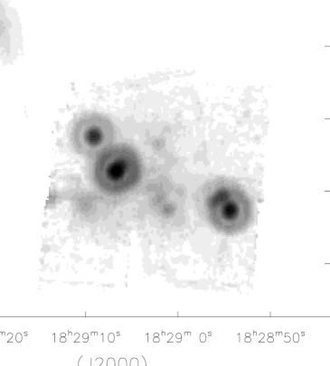
Figure 1: Spitzer MIPS fine-scale 70µm image of Cluster B (Serpens G3-G6 Cluster).

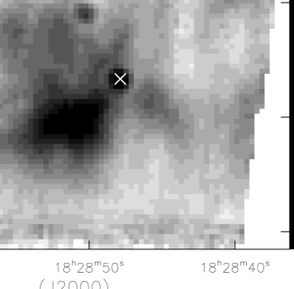
Figure 2: Spitzer MIPS fine-scale 70µm image of VV Ser. The nominal position of VV Ser is marked with the white ’X’.

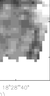
Figure 3: Spitzer MIPS 160µm image of VV Ser. The nominal position of VV Ser is marked with the white ’X’.

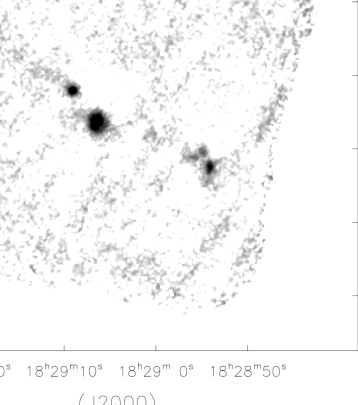
Figure 4: CSO SHARC-II 350µm image of Cluster B.

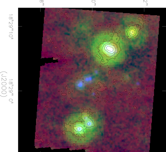
Figure 5: False color image of Cluster B with the 24µm image from the c2d data (blue), the 70µm fine-scale image from this study (green), and the SHARC-II 350µm image from this study (red). The contours of the 350µm data are overlaid on the image for clarity. The contours are logarithmically spaced at levels of $Log_{10}$ Surface Brightness (MJy/sr) = 2.5, 2.9, 3.3, and 3.7.

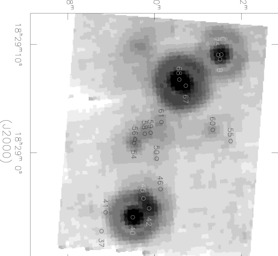
Figure 6: Image of the Cluster B region from figure 1 with the locations of the 19 YSO’s or candidates from Table 8 marked.

Figure 7: Contours of the $\chi^{2}$ values of the model fit for two closely spaced sources. The contours are at values of $\chi^{2}$ above the best-fit value by 0.5, 1.0, 2.3, and 5.0. Lines are drawn indicating the $\chi^{2}=2.3$ limits above the best fit value delimiting the uncertainties.

Figure 8: Lower panel: surface plot of our 70µm image of Cluster B, viewed roughly from the north. Upper panel: image with the point sources subtracted as described in the text. The maximum flux level is identical in both panels and is 2000 MJy/sr. Most of the residuals are well under 10% of the original image with the exception of some emission in the vicinity of sources 40, 42, and 45 that may be due to a slightly incorrect estimation of the PSF or to actual weak extended emission.

Figure 9: Plot of a 1-D cut through source C along a roughly east-west line (solid) versus the final assumed PSF (dash-dot).

Figure 10: Spectral energy distributions of the Cluster B YSO’s and candidates in Table 8 with the SED classification from Table 8 shown as well.

Figure 11: Left: Percent difference between $L_{bol}$ from Evans et al. (2008) and the new value of $L_{bol}$ from this study. Right: Percent difference between $T_{bol}$ from Evans et al. (2008) and the new value of $T_{bol}$ from this study.

References

- Backus et al. (2005) Backus, C., Velusamy, T., Thompson, T. & Arballo, J. 2005, ASPCS, 347, 61
- Beelen et al. (2006) Beelen, A., Cox, P., Benford, D.J., Dowell, C.D., Kovacs, A., Bertoldi, F., Omont, A., & Carilli, C. 2006, ApJ, 642, 694
- Chen et al. (1995) Chen, C.H., Myers, P.C., Ladd, E.F., & Wood, D.O.S. 1995, ApJ, 445, 377
- Djupvik et al. (2006) Djupvik, A.A., Andre,́ Ph., Bontemps, S., Motte, F., Olofsson, G., Galfalk, M. & Floren, H.-G. 2006,A&A, 458, 789
- Dowell et al. (2003) Dowell, C.D., et al. 2003, Proc. SPIE, 4855, 73
- Dunham et al. (2008) Dunham, M.M., Crapsi, A., Evans, N.J., II, Bourke, T.L., Huard, T.L., Myers, P.C., & Kauffmann, J. 2008, ApJS, in press
- Eiroa & Casali (1992) Eiroa, C. & Casali, M. M. 1992, A&A, 262, 468
- Eiroa, Djupvik & Casali (2008) Eiroa, C., Djupvik, A.A. & Casali, M.M. 2008, in Handbook of Star Forming Regions, Vol. II, (ASP Conf. Series), ed. B. Reipurth, in press
- Enoch et al. (2007) Enoch, M.L., Glenn, J., Evans, N.J., II, Sargent, A.I., Young, K.E., & Huard, T.L. 2007, ApJ, 666, 982
- Enoch et al. (2008) Enoch, M.L., et al. 2008, ApJ, in press, arXiv:0809.4012
- Enoch et al. (2009) Enoch, M.L. et al. 2009, in prep.
- Evans et al. (2003) Evans, N. J., II, et al. 2003, PASP, 115, 965
- Evans et al. (2007) Evans, N. J., II et al. 2007, Final Delivery of Data From the c2d Legacy Project: IRAC and MIPS, http://data.spitzer.caltech.edu/popular/c2d/20071101_enhanced_v1/ Documents/c2d_del_document.pdf
- Evans et al. (2008) Evans, N.J., II, et al. 2008, ApJ, submitted
- Gordon et al. (2007) Gordon, K.D. et al. 2007, PASP, 119, 1019
- Gutermuth et al. (2008) Gutermuth, R.A. et al. 2008, ApJ, 673L, 151
- Harvey, Wilking, & Joy (1984) Harvey, P. M., Wilking, B. A., & Joy, M. 1984, ApJ, 278, 156
- Harvey et al. (2006) Harvey, P.M. et al. 2006, ApJ, 644, 307
- Harvey et al. (2007a) Harvey, P.M. et al. 2007a, ApJ, 663, 1139
- Harvey et al. (2007b) Harvey, P.M., Merín, B., Huard, T.L., Rebull, L.M., Chapman, N., Evans, N.J. II & Myers, P.M. 2007b, ApJ, 663, 1149
- Kovács (2006) Kovács, A. 2006, Ph.D. thesis, California Institute of Technology
- Kovács et al. (2006) Kovács, A., Chapman, S.C., Dowell, C.D., Blain, A.W., Ivison, R.J., Smail, I., & Philiips, T.G. 2006, ApJ, 650, 592
- Lester et al. (1986) Lester, D.F, Harvey, P.M., Joy, M. & Ellis, H.B. 1986, ApJ, 309, 80
- Myers & Ladd (1993) Myers, P.C., & Ladd, E.F. 1993, ApJ, 413, L47
- Pontoppidan et al. (2007a) Pontoppidan, K. M. et al. 2007a, ApJ, 656, 980
- Pontoppidan et al. (2007b) Pontoppidan, K. M. et al. 2007b, ApJ, 656, 991
- Press et al. (1992) Press, W. H., Teukolsky, S. A., Vetterling, W. T., & Flannery, B. P. 1992, Numerical Recipes in C, Cambridge Univ. Press
- Rebull et al. (2007) Rebull, L. et al.(2007), ApJS, 171, 447
- Schechter, Mateo, & Saha (1993) Schechter, P. L., Mateo, M., & Saha, A. 1993, PASP, 105, 1342
- Shirley et al. (2000) Shirley, Y.L., Evans, N.J., II, Rawling, J.M.C., & Gregersen, E.M. 2000, ApJS, 131, 249
- Skemer et al. (2008) Skemer, A.J. et al. 2008, ApJ, in press
- Straizys, Cernis, & Bartasiute (1996) Straizys, V., Cernis, K., & Bartasiute, S. 1996, Balt. Astr, 5, 125
- Strom, Vrba & Strom (1976) Strom, S.E., Vrba, F. & Strom, K.M. 1976, AJ, 81, 638
- Wu et al. (2007)
- (35) Wu, J., Dunham, M.M., Evans, N.J., II, Bourke, T.L., & Young, C.H. 2007, AJ, 133, 1560