Oscillatory Notch pathway activity in a delay model of neuronal differentiation

Abstract

Lateral inhibition resulting from a double-negative feedback loop underlies the assignment of different fates to cells in many developmental processes. Previous studies have shown that the presence of time delays in models of lateral inhibition can result in significant oscillatory transients before patterned steady states are reached. We study the impact of local feedback loops in a model of lateral inhibition based on the Notch signalling pathway, elucidating the roles of intracellular and intercellular delays in controlling the overall system behaviour. The model exhibits both in-phase and out-of-phase oscillatory modes, and oscillation death. Interactions between oscillatory modes can generate complex behaviours such as intermittent oscillations. Our results provide a framework for exploring the recent observation of transient Notch pathway oscillations during fate assignment in vertebrate neurogenesis.

I Introduction

As in many electronic circuits, classes of oscillators and switches are fundamental elements in many gene regulatory networks TysonJJ03 ; KruseK05 . In particular, a double-negative feedback loop comprising two mutually repressive components is known to be capable of functioning as a toggle switch, allowing a system to adopt one of two possible steady states (corresponding to cell fates) CherryJL00 ; FerrellJE02 . In the context of developmental biology, such bistable switch networks can operate between cells, and are believed to drive cell differentiation in a wide range of contexts. However, in naturally evolved (rather than engineered) gene regulatory networks, double-negative feedback loops rarely exist in a “pure” form, and interactions between loop components and other network components often result in sets of interconnected feedback loops. Furthermore, if loop interactions involve the regulation of gene expression, then interactions are delayed rather than instantaneous. The present study investigates the dynamic behaviour of a double-negative feedback loop when the nodes of the loop are involved in additional feedback loops, and when the regulatory steps constituting the resulting network involve significant time delays.

A particularly well documented example of a biological double-negative feedback loop is centred on transmembrane receptors of the Notch family. Notch signalling, resulting from direct interaction with transmembrane ligands of the DSL (Delta, Serrate and Lag-2) family on neighbouring cells mediates an evolutionarily-conserved lateral inhibition mechanism that operates to specify differential cell fates during many developmental processes Artavanis-TsakonasS99 ; LewisJ98 ; LouviA06 ; RichardsGS08 . Although gene nomenclature varies between different organisms, a core circuitry—the neurogenic network—underlying lateral inhibition can be identified, and is illustrated schematically in Fig. 1 CollierJR96 ; MeirE02 . In brief, signalling between neighbouring cells is mediated by direct (juxtacrine) interactions between Notch receptors and DSL ligands. A double-negative feedback loop is formed by repression of DSL ligand activity by Notch signalling in the same cell (cell autonomous repression)—Fig. 1(a). Mathematical models of such a spatially-distributed double-negative feedback loop are capable of generating robust spatial patterns of Notch signalling in populations of cells CollierJR96 .

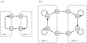
Figure 1: The neurogenic network models in a two-cell representation. The letters on the nodes correspond to the key classes of protein involved in the network — D: DSL ligand, N: Notch receptor, H: Hes/Her proteins, A: proneural proteins (e.g. Achaete, Scute, Neurogenin). Edges represent two types of directional interactions: activation ($\rightarrow$) and repression ($\multimap$). (a) The pure double-negative feedback loop involving only DSL ligand and Notch receptor CollierJR96 ; VeflingstadSR05 . (b) A more detailed model that incorporates Hes/Her negative feedback and proneural positive feedback MeirE02 .

In many developmental settings, the level of Notch signalling regulates the fate adopted by a cell by acting as an input to a cell autonomous bistable switch formed by one or more proneural genes (such as achaete and scute in Drosophila and neurogenin and atonal in vertebrates) BertrandN02 . The basic principle underlying this switch is the ability of the protein products of the proneural genes to positively regulate transcription of proneural genes, resulting in a direct positive feedback loop. In many systems, including the developing nervous system, Notch signalling regulates the proneural switch via regulation of the expression of proteins of the Hes/Her family. These proteins act as transcriptional repressors, and can repress their own expression and interfere with proneural self-activation KageyamaR07 . Furthermore, proneural proteins can also positively regulate the expression of DSL proteins, forming a complete circuit of interactions as shown in Fig. 1(b). Considered as an intercellular signalling network—which we shall refer to as the neurogenic network—this circuit comprises a spatially-distributed double-negative feedback loop with additional local positive and negative feedback loops.

A detailed mathematical model of the neurogenic network, incorporating Hes/Her negative feedback and proneural positive feedback, has been studied by Meir et al. MeirE02 , who showed by computer simulation that the network is capable of generating spatial patterns of Notch signalling in populations of cells. The models of Collier et al. CollierJR96 and Meir et al. MeirE02 incorporate the implicit assumption that all interactions are non-delayed. However, in reality the basic production mechanisms that regulate gene expression (gene transcription and mRNA translation) are associated with time delays MahaffyJM84 ; MahaffyJM88 . Incorporation of explicit time delays in the pure double-negative feedback loop shown in Fig. 1(a) results in competition between dynamic modes, with stable spatial patterning typically preceded by significant oscillatory transients VeflingstadSR05 . In a biological context, such transients would play an important role in delaying the onset of cell differentiation in a developing tissue. Delays can also generate oscillatory dynamics in models of Hes/Her negative feedback loops JensenMH03 ; LewisJ03 ; MonkNAM03 ; MomijiH08 , and such oscillations have been observed experimentally HirataH02 ; MasamizuY06 ; KageyamaR07 .

As predicted by mathematical models LewisJ03 ; VeflingstadSR05 , oscillatory expression of DSL ligands, Hes/Her proteins and proneural proteins has recently been observed in neural precursors in the developing mouse brain ShimojoH08 . Furthermore, these oscillations have been predicted to play a central biological role in delaying the onset of neural differentiation ShimojoH08 . In principle, these oscillations could be driven by the cell autonomous Hes/Her negative feedback loop, with Notch signalling providing coupling between cells LewisJ03 , or by the double-negative feedback loop centred on the DSL–Notch interaction VeflingstadSR05 . In the following, we investigate the interplay of local and intercellular feedback loops in models of the neurogenic network, using a combination of linear stability analysis and numerical simulations, emphasising the dynamical effects of the multiple time delays in the network. We study principally the case of two coupled cells, since this captures the essential features of oscillator synchronisation and cell state differentiation. We also show how our results extend to larger populations of coupled cells.

II The full Hes/Her–Proneural model and its dissection

In Fig. 1(b), positive regulation of Hes/Her (H) by proneural protein (A) in the adjacent cell, mediated by DSL–Notch signaling, can be considered simply as a cascade of three low-pass filters. This simplification allows the model in Fig. 1(b) to be reduced to the model in Fig. 2(a), where $\tau$ denotes time delay, and $f$ and $g$ represent generic increasing and decreasing functions, respectively. In this model, referred to hereafter as the full Hes/Her–Proneural model, Hes/Her proteins repress proneural proteins in the same cell (1 or 2), while proneural proteins activate Hes/Her proteins in the adjacent cell. This main loop is supplemented by the two local loops: Hes/Her auto-repression and proneural auto-activation. Each interaction is not instantaneous but involves a time delay, typically of the order of minutes to tens of minutes JensenMH03 ; LewisJ03 ; MonkNAM03 ; VeflingstadSR05 . The delays in the cell-autonomous regulatory steps ($\tau_{2}$–$\tau_{4}$) originate predominantly from processes associated with gene transcription, whereby the DNA sequence of a gene is transcribed into a corresponding mRNA molecule, while the delay in the non-cell-autonomous interaction ($\tau_{1}$) represents in addition processes involved in DSL–Notch signalling, such as protein processing NicholsJT07 .

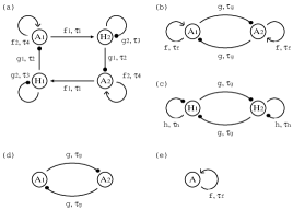
Figure 2: The neurogenic network models examined in the present study. $\tau$: time delays, $f$: a general increasing function; $g$, $h$: general decreasing functions. With an appropriate choice of time delay ($\tau_{1}$), the model in (a) provides a simplified representation of the full model shown in Fig. 1(b). The models in (a)–(d) have the potential to exhibit both oscillations and differentiation, while the model in (e) exhibits only differentiation.

The models in Fig. 2(b)–(e) are obtained by sequential reduction of the full neurogenic network. When Hes/Her feedback is negligible, the full Hes/Her–Proneural model in (a) becomes the model in (b); while when proneural feedback is negligible, the model in (a) becomes the model in (c). When both local loops are negligible, models (b) and (c) can be reduced to the model in (d). Finally, because two sequential repressions function as a net activation, the model in (d) can be further reduced to the model in (e). Such simple network elements appear repeatedly in gene regulatory networks (and possibly in other biological and non-biological networks), and are examples of what are often called “motifs” AlonU07 . The models in Fig. 2(b)–(e) are called hereafter: (b) the auto-activation two-Proneural model; (c) the auto-repression two-Hes/Her model; (d) the non-autonomous Proneural model; (e) the auto-activation single Proneural model.

III Mathematical representation of the full Hes/Her–Proneural model

We represent Hes/Her and proneural proteins by a single variable in each cell. To investigate the behaviour of a network quantitatively, it is convenient to scale each variable such that it lies in the range $[0,1]$. The full Hes/Her–Proneural model (Fig. 2(a)) can then be represented by the following differential equations with discrete delays:

$$T_{H}\ \dot{H}_{1} = -H_{1}+P_{H}(A_{2}(t-\tau_{1}),H_{1}(t-\tau_{3})),$$ (1)

$$T_{A}\ \dot{A}_{1} = -A_{1}+P_{A}(H_{1}(t-\tau_{2}),A_{1}(t-\tau_{4})),$$ (2)

$$T_{H}\ \dot{H}_{2} = -H_{2}+P_{H}(A_{1}(t-\tau_{1}),H_{2}(t-\tau_{3})),$$ (3)

$$T_{A}\ \dot{A}_{2} = -A_{2}+P_{A}(H_{2}(t-\tau_{2}),A_{2}(t-\tau_{4})),$$ (4)

where $T_{H}$ and $T_{A}$ denote the degradation constants (the inverses of the linear degradation rates) of $H$ and $A$, respectively MeirE02 . $P_{H}$ and $P_{A}$ are functions representing the rate of production of $H$ and $A$ respectively. The activating and repressive action of the proneural and Hes/Her proteins is captured by the following constraints:

$$\frac{\partial P_{H}}{\partial A} > 0,\quad\frac{\partial P_{H}}{\partial H}<0,$$ (5)

$$\frac{\partial P_{A}}{\partial A} > 0,\quad\frac{\partial P_{A}}{\partial H}<0.$$ (6)

For our analysis of this and the reduced models, we need assume no more about the production functions than the conditions (5) and (6). For numerical simulations, specific functional forms must be assumed, and we take these functions to be products of increasing ($f$) and decreasing ($g$ or $h$) Hill functions. Specifically, we assume that $P_{I}(A,H)=f_{I}(A)g_{I}(H)$ for $I=A$ or $H$, where

$$f_{I}(x,K,\nu) = \frac{x^{\nu}}{K^{\nu}+x^{\nu}},$$ (7)

$$g_{I}(x,K,\nu) = \frac{K^{\nu}}{K^{\nu}+x^{\nu}},$$ (8)

and $K$ and $\nu$ represent the scaled threshold and the Hill coefficient, respectively. However, the qualitative behaviour of the model solutions is preserved for other choices of production functions that satisfy conditions (5) and (6).

Numerical simulations of this model reveal a range of qualitatively different types of behaviour, in which oscillations can be absent, transient or sustained, and their phases can be locked or not (for examples, see Fig. 3). To investigate the origin of these behaviours, we reduce the full Hes/Her–Proneural model to a variety of simpler ones (see Fig. 2). The examination of these simpler networks (motifs) helps to elucidate the origins of the dynamics of the full Hes/Her–Proneural model.

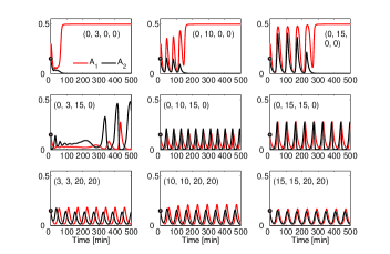
Figure 3: (Color online) Examples of typical dynamics found in numerical simulations of the full Hes/Her–Proneural model shown in Fig. 2(a) and defined by Eqs. 1–8, displaying both differentiation and oscillations. Oscillations can be transient or sustained, and can be in-phase between two cells, or not. Values of the kinetic parameters are set the same on each row and listed in Table 1. Delays are given in each panel as $(\tau_{1},\tau_{2},\tau_{3},\tau_{4})$

Table 1: Parameter values.

		$f_{H}$		$g_{H}$			$g_{A}$		$f_{A}$
	$T_{H}$	$K$	$\nu$	$K$	$\nu$	$T_{A}$	$K$	$\nu$	$K$	$\nu$
Standard	10	0.01	2	0.01	2	10	0.01	2	0.01	2
Fig. 3
Top	1	0.1	2	0.1	0	10	0.01	2	0.01	2
Middle	10	0.1	2	0.01	2	1	0.01	2	0	0
Bottom	10	0.01	2	0.01	2	10	0.01	2	0.01	2

IV Analysis and simulation of reduced models

In this study, we are concerned primarily with the routes that cells take to differentiation. For all model variants, a uniform steady state exists ($H_{1}^{*}=H_{2}^{*}$, $A_{1}^{*}=A_{2}^{*}$). Biologically, this corresponds to a non-differentiated state (i.e. the neurogenic network is in the same state in both cells). We therefore study the stability of this steady state to small perturbations, and seek to determine the resulting dynamical behaviour of the system in cases where it is unstable.

For each model variant (Fig. 2(b)–(e)), we first perform linear stability analysis of the uniform steady state, which yields an eigenvalue equation. We then determine parameter values that result in the existence of neutral (pure imaginary) eigenvalues, which are the product of the imaginary unit number and the neutral angular frequency, and are associated with changes in stability. To confirm the nature of bifurcations associated with these eigenvalues, the linear analysis is followed by numerical simulations. The eigenvalue equation for each model variant is derived directly from its own model equations, rather than by reduction of the full Hes/Her–Proneural model. The conditions under which the full Hes/Her–Proneural model can be reduced to the auto-activation two-Proneural model, and to the auto-repression two-Hes/Her model are discussed in Sect. VI.

To allow systematic comparison between model variants, we use a standard set of parameter values—which are listed in Table 1—in both analysis and simulations. These parameter values fall into a biologically reasonable range MeirE02 ; LewisJ03 and result in representative model dynamics. Deviations from this standard set are noted explicitly. Time is measured in minutes, yielding values for the degradation constants that are in line with measured values for proneural and neurogenic factors HirataH02 ; VosperJMD07 . However, the behaviour of each model variant is also examined with other parameter values.

In the following analyses, $\gamma$ denotes the magnitude of the slope of the regulatory function ($f_{j=1,2}(x)$ or $g_{j=1,2}(x)$) at the uniform steady-state solution ($H_{i=1,2}^{*}$ or $A_{i=1,2}^{*}$). In the cases of the Hill functions:

$$\gamma_{i=1,2}^{g_{j=1,2}} = -\frac{dg_{j=1,2}}{dx_{i}}|_{x_{i}^{*}}=\frac{\nu K^{\nu}{x_{i}^{*}}^{\nu-1}}{(K^{\nu}+{x_{i}^{*}}^{\nu})^{2}}>0,$$ (9)

$$\gamma_{i=1,2}^{f_{j=1,2}} = +\frac{df_{j=1,2}}{dx_{i}}|_{x_{i}^{*}}=\frac{\nu K^{\nu}{x_{i}^{*}}^{\nu-1}}{(K^{\nu}+{x_{i}^{*}}^{\nu})^{2}}>0,$$ (10)

where, in general, $K$ and $\nu$ are different in $f_{j=1,2}(x)$ and in $g_{j=1,2}(x)$, and therefore $\gamma_{i=1,2}^{g_{j=1,2}}\neq\gamma_{i=1,2}^{f_{j=1,2}}$. In the following sections, it can be seen that what determines the stability properties of the homogeneous steady state is not the precise functional forms of $f$ and $g$, but the value of $\gamma$.

IV.1 Non-autonomous two-Proneural model

The non-autonomous two-Proneural model (Fig. 2(d)) is represented by the following differential equations:

$$T\dot{A}_{1} = -A_{1}+g(A_{2}(t-\tau)),$$ (11)

$$T\dot{A}_{2} = -A_{2}+g(A_{1}(t-\tau)).$$ (12)

To study the stability of the uniform steady state solution ($A_{1}^{*}=A_{2}^{*}=A^{*}$), we set $A_{1}(t)=A^{*}+a_{1}(t)$ and $A_{2}(t)=A^{*}+a_{2}(t)$ in Eqs. (11) and (12). Following linearisation, the resulting coupled equations for $a_{1}$ and $a_{2}$ can be uncoupled by introducing variables $a_{1}+a_{2}$ and $a_{1}-a_{2}$ CollierJR96 . The eigenvalue equations derived from the equations in these variables are:

$$1+T\lambda=\pm\gamma\ e^{-\lambda\tau},$$ (13)

where the plus and minus branches are associated with $a_{1}-a_{2}$ and $a_{1}+a_{2}$ respectively.

We consider first uniform perturbations such that $a_{1}=a_{2}$. In this case, only the minus branch of Eq. (13) is relevant. Assuming a pure imaginary eigenvalue $\lambda=i\omega_{c}$, with $\omega_{c}$ real, the neutral angular frequency ($\omega_{c}$) is derived to be:

$$\omega_{c}=\frac{1}{T}\sqrt{\gamma^{2}-1}.$$ (14)

This eigenvalue occurs for parameter values such that $\gamma>1$ and when the delay is equal to the neutral delay $\tau_{c}$:

$$\tau_{c}=\frac{1}{\omega_{c}}\left(\pi+\tan^{-1}\left(-T\omega_{c}\right)\right).$$ (15)

For the standard set of parameter values (Table I), the oscillatory period associated with the neutral eigenvalue (the Hopf period)—defined by $T_{c}=2\pi/\omega_{c}$—is found to be 38.6501 min, while $\tau_{c}=13.0548$ min. For $\tau\neq\tau_{c}$, the minus branch of Eq. (13) has a complex eigenvalue with a real part that has the same sign as $\tau-\tau_{c}$. This can be seen in the numerical solution of Eq. (13) in Fig. 4.

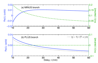
Figure 4: (Color online) The eigenvalues ($\lambda$) of the non-autonomous two-Proneural model (Fig. 2(d)) as a function of delay ($\tau$). The eigenvalue equation (Eq. (13)) has two branches. (a) On the minus branch $Re(\lambda)$ changes its sign from negative to positive as $\tau$ surpasses its critical value ($\tau_{c}=13.0548$), leading to a Hopf bifurcation, (b) while on the plus branch it is always positive. The minus and plus branches therefore define respectively the oscillatory and differentiating properties of the system. The dotted line in (b) shows the approximate analytical value for the real part of the eigenvalue derived in Eq. (17).

The linear stability analysis suggests that the uniform steady state becomes unstable to small uniform perturbations via a Hopf bifurcation if $\gamma>1$ and the delay increases above the critical value. Numerical simulations of Eqs. (11) and (12) for $\tau>\tau_{c}$ are shown in Fig. 5. For uniform initial conditions ($A_{1}(0)=A_{2}(0)$) the system exhibits sustained oscillations (Fig. 5(a)). This confirms that the neutral solution on the minus branch of Eq. (13) is a Hopf bifurcation point.

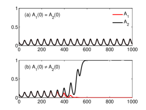
Figure 5: (Color online) Numerical simulations of the non-autonomous two-Proneural model (Fig. 2(d)). (a) With identical initial values, $A_{1}$ and $A_{2}$ show sustained in-phase oscillations. (b) With slightly different initial values, $A_{1}$ and $A_{2}$ show transient in-phase oscillations followed by differentiation (cf. VeflingstadSR05 ). Standard parameter values are used, as listed in Table 1, with $\tau=20$ min.

The plus branch of Eq. (13)—which is associated with $a_{1}-a_{2}$—has the same neutral angular frequency ($\omega_{c}$) as the minus branch, and the neutral eigenvalue occurs for a neutral delay $\tau_{c}$:

$$\tau_{c}=\frac{1}{\omega_{c}}\tan^{-1}\left(T\omega_{c}\right),$$ (16)

which takes value 6.2702 min for the standard parameter set. More generally, the real part of a complex eigenvalue $\lambda_{+}$ satisfies

$$1+T\ Re(\lambda_{+})=\gamma\ e^{-Re(\lambda_{+})\tau}\cos(Im(\lambda_{+})\tau).$$

Since $Re(\lambda_{+})$ is given by the intersection of $y=1+TRe(\lambda_{+})$ and $y=\gamma\exp(-Re(\lambda_{+})\tau)\cos(Im(\lambda_{+})\tau)$ on the $y$–$Re(\lambda_{+})$ plane, a purely real $\lambda_{+}$ (for which $\cos(Im(\lambda_{+})\tau)=1$) has the largest real part, and is positive for all values of $\tau$ if $\gamma>1$. This positive real eigenvalue is shown in Fig. 4(b). By assuming a purely real eigenvalue $(\lambda_{R+})$, and by applying the first-order Taylor expansion to Eq. (13), a simple approximate (lower bound) expression for $\lambda_{R+}$ is derived to be

$$\lambda_{R+}\simeq\frac{\gamma-1}{T+\gamma\tau},$$ (17)

which is confirmed to provide a good approximation to the growth rate of patterns obtained in numerical simulations in Fig. 4(b). Previously, such an approximation was thought to be possible only in the limit of a large Hill coefficient ($\nu$) VeflingstadSR05 , while in Fig. 4, $\nu=2$.

The positive real eigenvalue on the plus branch corresponds to differentiation of the two cells (exponential growth of $a_{1}-a_{2}$), while the complex eigenvalue associated with the minus branch corresponds to oscillations (in $a_{1}+a_{2}$). Thus, if $A_{1}(0)$ and $A_{2}(0)$ are set slightly different, the behaviour of the system comprises a combination of these two fundamental modes. This can be seen in the numerical simulation of Eqs. (11) and (12) in Fig. 5(b), which shows a transient uniform oscillation followed by differentiation. Since the oscillations occur on the minus branch corresponding to $a_{1}+a_{2}$, the oscillatory profiles of $A_{1}$ and $A_{2}$ are in-phase. Similar transient oscillations leading to differentiation have been observed previously in a delay model of the Delta-Notch signalling system (Fig. 1(a)) VeflingstadSR05 .

In general, the outcome of linear stability analysis is not applicable to transient system behaviour. Therefore, the separation of the two branches makes linear analysis highly valuable in this study, making possible the prediction of whether or not a transient oscillation leading to differentiation occurs. More striking is the fact that not only the initial rate of differentiation, but also the time taken to complete differentiation can be estimated by linear analysis. Fig. 6 shows the time-courses of the (logarithmic) difference $A_{2}-A_{1}$ obtained from numerical simulations for a range of values of the delay ($\tau$) and initial mean values ($A_{0}=0.5\left[A_{2}(0)+A_{1}(0)\right]$). These are compared to the growth rate predicted by the real part of the eigenvalue for $a_{2}-a_{1}$ (i.e. the plus branch), obtained from linear analysis for the corresponding $\tau$ (Fig. 4), which provides a good estimate of the time taken to reach the fully differentiated state.

(a)
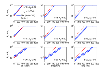
(b)

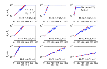
Figure 6: (Color online) Time taken for differentiation in the non-autonomous two-Proneural model (Fig. 2(d)). Time courses of the difference $A_{2}-A_{1}$—obtained from numerical simulations—plotted on a logarithmic scale, (a) for various delays ($\tau$) and initial mean values ($A_{0}=0.5\left[A_{2}(0)+A_{1}(0)\right]$) with the standard parameter set, and (b) for various parameter sets with $\tau=1.5\ \tau_{c}(H,K,\nu)$, where $\tau_{c}$ is the critical delay. The time courses are compared to the growth rate predicted from linear analysis (dashed line), based on the real part of the eigenvalue ($Re(\lambda)$).

IV.2 Auto-activation single Proneural model

Because two sequential repressions result in a net activation, the non-autonomous two-Proneural model (Fig. 2(d)) may seem to be surrogated by the auto-activation single Proneural model (Fig. 2(e)), represented by the following differential equation:

$$T\dot{A} = -A+f(A(t-\tau_{f})).$$ (18)

The eigenvalue equation obtained by linearisation about a steady state of Eq. (18), is

$$1+T\lambda=\gamma\ e^{-\lambda\tau},$$

which is identical to the plus branch of Eq. (13) that represents the differentiating nature of the non-autonomous two-Proneural model. It is therefore clear that the oscillation in the two-Proneural model is due to the network structure that two proneural proteins are mutually repressing.

IV.3 Auto-activation two-Proneural model

The auto-activation two-Proneural model (Fig. 2(b)) is represented by the following differential equations:

$$T\dot{A}_{1} = -A_{1}+g(A_{2}(t-\tau_{g}))\ f(A_{1}(t-\tau_{f})),$$ (19)

$$T\dot{A}_{2} = -A_{2}+g(A_{1}(t-\tau_{g}))\ f(A_{2}(t-\tau_{f})).$$ (20)

The eigenvalue equation for the uniform steady-state solution ($A_{1}^{*}=A_{2}^{*}=A^{*}$) is derived to be:

$$1+T\lambda=g(A^{*})\gamma^{f}e^{-\lambda\tau_{f}}\pm f(A^{*})\gamma^{g}e^{-\lambda\tau_{g}}.$$ (21)

The purely imaginary solution $\lambda=i\omega$ satisfies:

$$1+B^{2}-C^{2}+T^{2}\omega^{2}+2B(T\omega\sin\omega\tau_{f}-\cos\omega\tau_{f})=0,$$ (22)

where $B=g(A^{*})\gamma^{f}$ and $C=f(A^{*})\gamma^{g}$.

Fig. 7 shows the neutral intercellular signalling delay and corresponding oscillatory period, associated with the pure imaginary eigenvalues, as a function of local-loop delay ($\tau_{f}$). The eigenvalue equation (Eq. (21)) is solved for its minus and plus branches. As $\tau_{f}$ is varied, the values of the neutral intercellular signalling delay and the neutral oscillatory period fluctuate, with the oscillatory period fluctuating around its value in the non-autonomous two-Proneural model (Fig. 2(d)). A similar modulation in period was recently observed in a delayed coupling model of vertebrate segmentation MorelliLG09 . Numerical simulations performed for the parameter values represented by the cross signs in Fig. 7(a) confirm that the Hopf bifurcation occurs on the minus branch of Eq. (21), and that the critical intercellular signalling delay is modulated by the local-loop delay (data not shown).

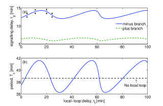
Figure 7: (Color online) Neutral intercellular signalling delay (a) and oscillatory period (b) associated with the pure imaginary eigenvalues of the auto-activation two-Proneural model (Fig. 2(b)), shown as a function of local-loop delay ($\tau_{f}$). The eigenvalue equation (Eq. (21)) is solved numerically for its minus and plus branches. The Hopf bifurcation occurs on the minus branch. Also shown in (b) is the corresponding Hopf period for the non-autonomous two-Proneural model, which lacks the local (cell-autonomous) proneural feedback loops (Fig. 2(d)). Numerical simulations performed for parameter values corresponding to the cross signs in (a) confirm that the Hopf bifurcation occurs on the minus branch of Eq. (21), and that the critical intercellular signalling delay ($\tau_{g}$) is modulated by $\tau_{f}$.

Fig. 8 shows the results of numerical simulations of the model equations (19) and (20) for a range of delays ($\tau_{g}$ and $\tau_{f}$) and initial values ($A_{1}(0)$ and $A_{2}(0)$). The behaviour of this model variant is found to be qualitatively the same as that of the non-autonomous two-Proneural model (Fig. 2(d)): the Hopf bifurcation point exists on the minus branch of the eigenvalue equation (Eq. (21)) and, since the plus branch again has a positive real eigenvalue, differentiation occurs when $A_{1}(0)\neq A_{2}(0)$. However, the modulatory effect of the cell-autonomous proneural auto-activation loop, shown in Fig. 7, is seen in the comparison between top and the middle right panels. As the local-loop delay ($\tau_{f}$) increases from 0 to 15, the amplitude of oscillations decreases, influenced by the increase of the critical signalling delay (Fig. 7(a), solid curve). It can be seen from Fig. 7 that the cell-autonomous proneural auto-activation loops give rise to ‘tunability’ of the oscillations.

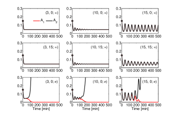
Figure 8: (Color online) Numerical simulations of the auto-activation two-Proneural model (Fig. 2(b)). In comparison to Fig. 5, the behaviour is found to be qualitatively the same as that of the non-autonomous two-Proneural model (Fig. 2(d)). However, the modulatory effect of the cell-autonomous proneural loop, shown in Fig. 7, is seen in the comparison between top and the middle right panels. As the local-loop delay ($\tau_{f}$) increases from 0 to 15, the amplitude of oscillations decreases, influenced by the increase of the critical signalling delay (Fig. 7(a), solid curve). Values of the delays, and whether or not the initial values of $A_{1}$ and $A_{2}$ are equal, are specified in each panel as $(\tau_{g},\tau_{f};=\text{ or }\neq)$.

IV.4 Auto-repression two-Hes/Her model

The auto-repression two-Hes/Her model (Fig. 2(c)) is represented by the following differential equations:

$$T\dot{H}_{1} = -H_{1}+g(H_{2}(t-\tau_{g}))\ h(H_{1}(t-\tau_{h})),$$ (23)

$$T\dot{H}_{2} = -H_{2}+g(H_{1}(t-\tau_{g}))\ h(H_{2}(t-\tau_{h})).$$ (24)

The eigenvalue equation for the uniform steady-state solution ($H_{1}^{*}=H_{2}^{*}=H^{*}$) has the same form as that for the auto-activation two-Proneural model (Eq. (21)):

$$1+T\lambda=-g(H^{*})\gamma^{h}e^{-\lambda\tau_{h}}\pm h(H^{*})\gamma^{g}e^{-\lambda\tau_{g}},$$ (25)

where, however, the definition of $B$ is modified to be $B=-g(H^{*})\gamma^{h}$ because $h$ represents a decreasing Hill function.

Fig. 9 shows the neutral intercellular signalling delay and oscillatory period associated with the pure imaginary eigenvalues, as a function of the delay in the local loop. The eigenvalue equation (Eq. (25)) is solved for its minus and plus branches, for the first and the second largest periods. Unlike any eigenvalue equation of the three simpler models analysed so far (Fig. 2(b), (d) and (e)), Eq. (25) is found not to have a neutral solution when $\tau_{h}<5.0483$ min.

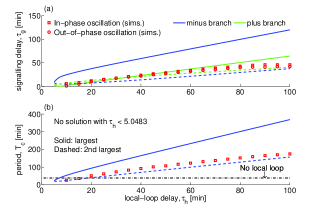
Figure 9: (Color online) Neutral intercellular signalling delay (a) and oscillatory period (b) associated with the pure imaginary eigenvalues of the auto-repression two-Hes/Her model (Fig. 2(c)), shown as a function of the local-loop delay. The eigenvalue equation (Eq. (25)) is solved for its minus and plus branches, for the first and the second largest periods (solid and dashed lines, respectively). This model shows the transition between out-of-phase and in-phase oscillations. At each local-loop delay, a square represents the in-phase oscillation observed in simulation with the lowest signalling delay, while a circle represents the out-of-phase oscillation observed in simulation with the highest signalling delay. The transition happens between them (upper panel), which are overlapping with a square being always above a circle.

Numerical simulations of the model equations (23) and (24) reveal two prominent features of the dynamics of this system that are qualitatively different to those of the two-Proneural models (Figs. 2(b),(d)). Fig. 10 shows simulation results for a range of values of the delays ($\tau_{g}$ and $\tau_{h}$) and initial values ($H_{1}(0)$ and $H_{2}(0)$). Two new features are apparent: first, oscillations can be sustained (rather than transient) even when $H_{1}(0)\neq H_{2}(0)$; second, the oscillations of $H_{1}$ and $H_{2}$ can be out-of-phase for certain values of the delays, as shown in the left bottom panel. Fig. 11 details the transition from out-of-phase oscillations to in-phase oscillations as the value of the critical intercellular signalling delay ($\tau_{g}$) increases. Strikingly, the transition is found to be associated with a point-wise amplitude death ReddyDVR98 . The transition found in numerical simulations with various $\tau_{h}$ is compared to the neutral properties estimated by the linear analysis in Fig. 9. In a cell-autonomous Hes/Her oscillator, the oscillatory period increases monotonically with delay MonkNAM03 , while for the coupled cells to cycle out-of-phase, the signalling delay must be about half a period. Therefore the monotonic increase in the critical $\tau_{g}$ and in the critical period ($T_{c}$) suggests that the overall network behaviour of the auto-repression two-Hes/Her model is controlled by the two local autonomous Hes/Her oscillators.

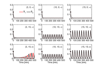
Figure 10: (Color online) Numerical simulations of the auto-repression two-Hes/Her model (Fig. 2(c)). In comparison to Fig. 5, the behaviour is found to be qualitatively different to that of the non-autonomous two-Proneural model (Fig. 2(d)). Specifically, oscillations are sustained even with non-identical initial values, and oscillations can be out-of-phase as well as in-phase. Values of the delays, and whether or not the initial values of $H_{1}$ and $H_{2}$ are equal, are specified in each panel as $(\tau_{g},\tau_{h};=\text{ or }\neq)$.

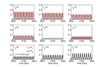
Figure 11: (Color online) Detail of the transition from out-of-phase to in-phase oscillations as the value of $\tau_{g}$ increases in the auto-repression two-Hes/Her model (Fig. 2(c); Fig. 10). The transition is associated with amplitude death around $\tau_{g}=6$.

In contrast, when the intercellular signalling delay ($\tau_{g}$) is varied while the local delay ($\tau_{h}$) is kept constant, transitions between in-phase and out-of-phase modes occur sequentially, and are associated with modulations in amplitude and period (Fig. 12). The mode transitions repeat as $\tau_{g}$ is increased, but not in an identical manner. Unlike the first transition shown in Fig. 11, a clear amplitude death is not observed at higher-order transitions. Further examination reveals that the sequential transitions are not induced by the network structure of two mutually repressive autonomous oscillators, but by the structure of two mutually influencing autonomous oscillators, forming an overall positive feedback loop. Indeed, when intercellular interactions are modelled by an increasing Hill function that represents activation, the transition still occurs, but in a reverse order, starting from the in-phase mode at $\tau_{g}=0$ (data not shown).

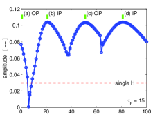
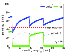
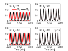
Figure 12: (Color online) Dependence of the amplitude (top panel) and period (middle panel) of oscillatory solutions on the intercellular signalling delay ($\tau_{g}$) in the auto-repression two-Hes/Her model. The amplitude of an oscillatory solution is defined as the half difference between peak and trough values. The observed modulations of amplitude and period reflect the transition between out-of-phase (OP) and in-phase (IP) oscillation modes; the comparison between lag (time difference between oscillation peaks in neighbouring cells) and the half-period of oscillations shown in the middle panel illustrates the sequential switching between out-of-phase and in-phase oscillation modes. The bottom four panels show time courses obtained by numerical simulation of Eqs. (23) and (24) at the four values of $\tau_{g}$ marked in the top panel. The first transition corresponds to Fig. 11. The dashed lines in the top and the middle panels represent respectively the amplitude and the period in the single-cell Hes/Her model with local delay $\tau_{h}=15$.

The intercellular coupling is found to have additional dynamical consequences. While an isolated cell containing the Hes/Her feedback loop cannot exhibit sustained oscillations when the delay ($\tau_{h}$) is below its critical value, such a local-loop critical delay ($\tau_{h\ cr}$) can be lowered by the intercellular coupling, as shown in Fig. 13, where $\tau_{h}=10<\tau_{h\ cr}=13.0548$. Furthermore, oscillation death is found to happen in a definite range of the intercellular signalling delay ($\tau_{g}$).

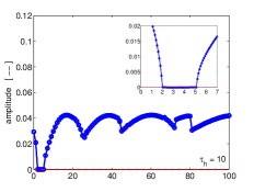
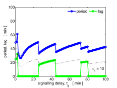
Figure 13: (Color online) Coupled sub-critical oscillators illustrating a finite-$\tau_{g}$-range oscillation death. The inset in the top panel shows the oscillation death in detail.

The three features observed in numerical simulations—the oscillation in an originally subcritical delay range ($\tau_{h}<\tau_{h\ cr}$), the transition between out-of-phase and in-phase oscillatory modes, and the finite-$\tau_{g}$-range oscillation death—can be understood analytically as follows. Linearisation of Eqs. (23) and (24) around the uniform steady state yields:

$$\left(\begin{array}[]{cc}1+T\lambda+\alpha&\beta\\ \beta&1+T\lambda+\alpha\end{array}\right)\left(\begin{array}[]{c}\bar{H}_{1}\\ \bar{H}_{2}\end{array}\right)=\mathbb{M}\left(\begin{array}[]{c}\bar{H}_{1}\\ \bar{H}_{2}\end{array}\right)=\left(\begin{array}[]{c}0\\ 0\end{array}\right),$$ (26)

where $\alpha=g(H^{*})\gamma^{h}e^{-\lambda\tau_{h}}$, $\beta=h(H^{*})\gamma^{g}e^{-\lambda\tau_{g}}$. The associated eigenvalue equation, given by $\det\mathbb{M}=0$, is:

$$1+T\lambda=-\alpha\pm\beta,$$ (27)

which is the same as Eq. (25). By substituting Eq. (27) into Eq. (26), it can be seen that the plus branch is associated with the out-of-phase oscillation mode: $(\bar{H}_{1},\bar{H}_{2})=(1,-1)$, whereas the minus branch is associated with the in-phase oscillation mode: $(\bar{H}_{1},\bar{H}_{2})=(1,1)$. Numerical evaluation of the eigenvalue equation yields the relations between the neutral delay in the local loop ($\tau_{h\ cr}$) and the intercellular signalling delay ($\tau_{g}$) shown in Fig. 14, for both the out-of-phase (green) and the in-phase (blue) modes. For example, for $\tau_{h}=10$ (Fig. 13), when $0<\tau_{g}<2$ only the out-of-phase mode is allowed, whereas when $\tau_{g}\geq 5.1$ only the in-phase mode is allowed. In between ($2<\tau_{g}<5.1$), no oscillation is allowed, explaining the origin of the oscillation death shown in Fig. 13. However, the comparison of periods to simulation results in the lower panel shows that as $\tau_{g}$ increases, more and more branches appear, and the model behaviour becomes more non-linear. The actual transitions observed in simulations do not coincide with the boundaries between the regions that linear stability analysis predicts to be competent (solid) and incompetent (dashed) for sustained oscillations.

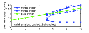
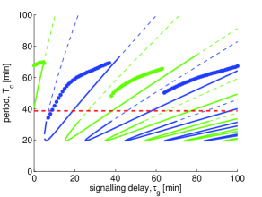
Figure 14: (Color online) The origin of oscillation death, and the transition between the out-of-phase and the in-phase oscillatory modes in the auto-repression two-Hes/Her model (Fig. 2(c)). Neutral local-loop delay (upper panel) and oscillatory period (lower panel) are shown as functions of the intercellular signalling delay $\tau_{g}$. The eigenvalue equation (Eq. (25)) is solved numerically for its minus and plus branches. Neither the out-of-phase branch (green) nor the in-phase branch (blue) have a solution for $\tau_{h}=10$ for $2\leq\tau_{g}<5.1$, corresponding to the oscillation death observed in Fig. 13. Simulated periods for $\tau_{h}=15$ (shown also in Fig. 12, middle panel) are shown by blue and green dots in the lower panel, where the neutral period obtained by linear stability analysis is shown by solid and dashed curves (correspond to the neutral delay being smaller or larger than $\tau_{h}=15$, respectively). Note the different horizontal scales in the two panels.

It is striking that only by changing the local loop attached to the non-autonomous two-X model from auto-activation (Fig. 2(b) where X is Proneural) to auto-repression (Fig. 2(c) where X is Hes/Her), the network behaviour changes completely. This simple example, motivated by the structure of the neural differentiation network, highlights the importance of examining in detail the structure of any gene regulatory network, even if it is centred on a small and seemingly simple motif.

Richness in the behaviour of this auto-repression two-Hes/Her model can be seen in Fig. 15, where the largest neutral period ($T_{c}$) associated with the eigenvalues is plotted for different values of thee threshold ($K_{h}$) and Hill coefficient ($\nu_{h}$) in the local feedback loop. As $K_{h}$ increases, the behaviour of this model becomes similar to that of the auto-activation two-Proneural model (Fig. 2(b)), while as $\nu_{h}$ decreases, the behavour becomes similar to that of the non-autonomous two-Proneural model (Fig. 2(d)).

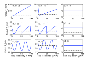
Figure 15: (Color online) The largest neutral period ($T_{c}$) associated with the eigenvalues of the auto-repression two-Hes/Her model (Fig. 2(c)) for different values of the threshold ($K_{h}$) and the Hill coefficient ($\nu_{h}$) in the local feedback loop. As $K_{h}$ increases, the behaviour of this model becomes similar to that of the auto-activation two-Proneural model (Fig. 2(b)), while as $\nu_{h}$ decreases, the behavour becomes similar to that of the non-autonomous two-Proneural model (Fig. 2(d)). Note the different vertical scales in each plot. The dashed-dot line in each panel represents the critical period in the non-autonomous two-cell model. Varied parameters are given in each panel as ($K_{h}$, $\nu_{h}$).

V Extension to $N$-cell ring model

The two-cell models discussed so far can be naturally extended to one-dimensional arrays of cells. To avoid potential boundary effects, we consider the specific case of a ring of $N$ cells labelled with a single index $i=1,2,\ldots,N$ (i.e. a line of cells with periodic boundary conditions imposed). As an example, we study the auto-repression Hes/Her model. We assume that each cell signals equally to both its nearest neighbours, yielding the following model equations:

$$T\ \dot{H}_{i}=-H_{i}+h(H_{i}(t-\tau_{h}))\ g\left(\frac{H_{i-1}(t-\tau_{g})+H_{i+1}(t-\tau_{g})}{2}\right),$$ (28)

where $i$ denotes cell number and the imposition of periodic boundary conditions implies that $H_{-1}=H_{N}$ and $H_{N+1}=H_{1}$. Linearising Eq. (28) around the uniform steady-state solution ($H_{i}=H^{*}$) by expanding $H_{i}$ as $H_{i}=H^{*}+\bar{H}_{i}e^{\lambda t}$ yields the following eigenvalue equations:

$$0=A\bar{H}_{i-1}+(B-\lambda T)\bar{H}_{i}+A\bar{H}_{i+1},\quad i=1,2,\ldots,N,$$ (29)

where

$$A(\lambda) = -\frac{1}{2}h(H^{*})\gamma^{g}e^{-\lambda\tau_{g}},$$

$$B(\lambda) = -1-g(H^{*})\gamma^{h}e^{-\lambda\tau_{h}}.$$

Eq. (29) can be represented in matrix form as:

$$\left(\begin{array}[]{c}0\\ 0\\ 0\\ \\ \vdots\\ \\ 0\end{array}\right)=\left(\begin{array}[]{ccccccccc}B-\lambda T&A&0&0&0&\cdots&0&0&A\\ A&B-\lambda T&A&0&0&\cdots&0&0&0\\ 0&A&B-\lambda T&A&0&\cdots&0&0&0\\ \\ &&&&\cdots&&&&\\ \\ A&0&0&0&0&\cdots&0&A&B-\lambda T\end{array}\right)\left(\begin{array}[]{c}\bar{H}_{1}\\ \bar{H}_{2}\\ \bar{H}_{3}\\ \\ \vdots\\ \\ \bar{H}_{N}\end{array}\right)=\mathbb{M}\left(\begin{array}[]{c}\bar{H}_{1}\\ \bar{H}_{2}\\ \bar{H}_{3}\\ \\ \vdots\\ \\ \bar{H}_{N}\end{array}\right),$$ (30)

where it is important to note that $A$ and $B$ are non-polynomial functions of $\lambda$. The eigenvalues $\lambda$ are determined by $\det\mathbb{M}=0$.

We first note that the phase relations between adjacent cells in oscillatory solutions can be determined from the form of the eigenvector $(\bar{H}_{1},\bar{H}_{2},\ldots\bar{H}_{N})$ corresponding to each eigenvalue. For any value of $N$, Eq. (30) has an eigenvector $(1,1,\ldots,1)$ with an eigenvector determined by the solutions of $T\lambda=B+2A$. This corresponds to an oscillatory mode where all cells are in-phase. Furthermore, for any even value of $N$, Eq. (30) has an eigenvector $(1,-1,1,\ldots,1,-1)$ with an eigenvector determined by the solutions of $T\lambda=B-2A$. This corresponds to an oscillatory mode where all cells are out-of-phase. These two cases are simple extensions of the dynamics observed in the two cell model.

To illustrate potential extensions to the dynamics observed in the two cell model, we consider the specific case $N=4$:

$$\mathbb{M}=\left(\begin{array}[]{ccccccccc}B-\lambda T&A&0&A\\ A&B-\lambda T&A&0\\ 0&A&B-\lambda T&A\\ A&0&A&B-\lambda T\end{array}\right),$$ (31)

and

$$\det\mathbb{M}=(-2A+T\lambda-B)(2A+T\lambda-B)(-B+T\lambda)^{2}.$$

Therefore, the eigenvalues are determined by the solutions of:

$$T\lambda = B\mp 2A,$$ (32)

$$T\lambda = B.$$ (33)

The explicit expression of Eqs. (32) and (33) are found to be the same as the eigenvalue equations derived for the auto-repression two-Hes/Her model (Eq. (25)), and for the auto-repression single Hes/Her model (the minus branch of Eq. (13)), respectively.

As above, the phase relations between adjacent cells in oscillatory solutions can be determined from the form of the eigenvector $(\bar{H}_{1},\bar{H}_{2},\bar{H}_{3},\bar{H}_{4})$ corresponding to each eigenvalue. From Eq. (31), the eigenvector on the minus branch of Eq. (32) is found to be $(1,-1,1,-1)$, representing the out-of-phase oscillatory mode, while the eigenvector on the plus branch is $(1,1,1,1)$, representing the in-phase mode. In contrast, the eigenvector associated with Eq. (33), which is present when $N=4,8,16,\ldots$, is found to be $(1,0,-1,0)$, representing amplitude death for every other cell in the array, with the remaining cells being out-of-phase. This is a new dynamical feature that the two-cell model fails to capture. An example of this mode for $N=4$ is shown in Fig. 16(a).

For larger values of $N$, interaction between multiple modes can result in more complex oscillatory behaviour, in which waves of phase and amplitude differences can propagate around the ring. Furthermore, the oscillatory profile for each cell is often complex, with multiple peaks per oscillatory period and “intermittent” oscillations being common. An example for $N=7$ is shown in Fig. 16(b). These features are also observed in simulations on regular square and hexagonal two-dimensional arrays of cells (results not shown).

(a)
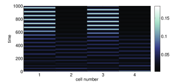
(b)

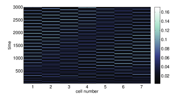
Figure 16: Complex oscillatory dynamics in one-dimensional arrays of coupled cells. Simulations of Eqs. (28), representing the the auto-repression Hes/Her model in a ring of $N$ cells. Simulations were carried out using the standard parameter values (Table 1) with $\tau_{h}=20$, $\tau_{g}=8$ and with initial history $H_{i}(t)=0.1+0.1\xi_{i}$ for $-\textrm{max}(\tau_{g},\tau_{h})\leq t\leq 0$, where the $\xi_{i}$ are drawn from independent uniform distributions on $[0,1]$ (a) Amplitude death combined with out-of-phase oscillations: $N=4$. (b) Complex dynamics resulting from mode interactions: $N=7$.

VI Analysis and reductions of the full Hes/Her–Proneural model

In this section, from the viewpoint of eigenvalue equations, it is discussed how the full Hes/Her–Proneural model (Fig. 2(a)) is related to the auto-activation Proneural model (Fig. 2(b)), and to the auto-repression Hes/Her model (Fig. 2(c)).

For the uniform steady-state solution ($H_{1}^{*}=H_{2}^{*}=H^{*}$, $A_{1}^{*}=A_{2}^{*}=A^{*}$) of the full Hes/Her–Proneural model, the eigenvalue equation is derived from its model equations (1)–(4) to be:

$$(1+T_{H}\lambda+ae^{-\lambda\tau_{3}})(1+T_{A}\lambda-ce^{-\lambda\tau_{4}})=\pm bde^{-\lambda\tau_{tot}},$$ (34)

where $a=f_{1}(A^{*})\gamma^{g_{2}}$, $b=f_{2}(A^{*})\gamma^{g_{1}}$, $c=g_{1}(H^{*})\gamma^{f_{2}}$, $d=g_{2}(H^{*})\gamma^{f_{1}}$, and $\tau_{tot}=\tau_{1}+\tau_{2}$.

First, explicit forms of the neutral angular frequency ($\omega_{c}$) and delay ($\tau_{tot}$) are derived for a simple example, where $T_{A}=T_{H}=T$, $\tau_{3}=\tau_{4}=\tau_{a}$, and $f_{1}=f_{2}=g_{1}=g_{2}$. The last assumption means that $K$ and $\nu$ are respectively the same all in $f_{1}$, $f_{2}$, $g_{1}$, and $g_{2}$. Then, from Eqs (9) and (10), $A^{*}=H^{*}$, and consequently $a=c=b=d:=\phi$. Therefore, Eq. (34) becomes:

$$1+2T\lambda+T^{2}\lambda^{2}-\phi^{2}e^{-2\lambda\tau_{a}} = \pm\phi^{2}e^{-\lambda\tau_{tot}}.$$ (35)

For a neutral solution, Eq. (35) becomes:

$$(1-T^{2}\omega^{2}-\phi^{2}\cos 2\omega\tau_{a})^{2}+(2T\omega+\phi^{2}\sin 2\omega\tau_{a})^{2}=\phi^{4},$$ (36)

$$\tan\omega\tau_{tot}=\mp\frac{2T\omega+\phi^{2}\sin 2\omega\tau_{a}}{1-T^{2}\omega^{2}-\phi^{2}\cos 2\omega\tau_{a}}:=\mp\Delta.$$ (37)

For the plus branch in Eq. (34):

$$\tau_{tot}=\frac{1}{\omega}\max[\ \tan^{-1}(-\Delta),\ \pi+\tan^{-1}(-\Delta)\ ],$$ (38)

whereas for the minus branch in Eq. (34):

$$\tau_{tot}=\frac{1}{\omega}\max[\ \tan^{-1}(+\Delta),\ \pi+\tan^{-1}(+\Delta)\ ].$$ (39)

Fig. 17 shows the neutral (a) intercellular signalling delay and (b) period, as a function of the local-loop delay ($\tau_{a}$). The eigenvalue equation (Eq. (35)) is solved for its minus and plus branches, for the first and the second largest periods. In comparison to Figs. 7 and 9, the auto-repression two-Hes/Her circuit component is found to be dominant in this full Hes/Her-Proneural model, although the neutral values are found to exist for any $\tau_{a}$, unlike in the auto-repression two-Hes/Her model, where no pure imaginary solution can exist for $\tau_{f}$ less than 5.0483 ($\tau_{f}$ corresponds to $\tau_{a}$ in this section).

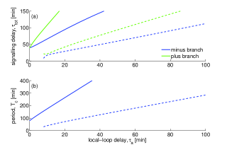
Figure 17: (Color online) Neutral (a) intercellular signalling delay and (b) period, associated with the pure imaginary eigenvalues of the full Hes/Her-Proneural model, shown as a function of the local-loop delay. The eigenvalue equation (Eq. (35)) is solved for its minus and plus branches, for the first and the second largest periods (solid and dashed lines, respectively). In comparison to Figs. 7 and 9, the auto-repression two-Hes/Her circuit component is found to be dominant in this full Hes/Her-Proneural model.

In the following, based on the eigenvalue equation of the full Hes/Her–Proneural model (Eq. (34)), we clarify the conditions under which this full Hes/Her–Proneural model can be reduced to the auto-activation two-Proneural model (Fig. 2(b)), and to the auto-repression two-Hes/Her model (Fig. 2(c)).

VI.1 Reduction to the auto-activation two-Proneural model

The eigenvalue equation of the full Hes/Her–Proneural model (Eq. (34)) is reduced to the eigenvalue equation of the auto-activation two-Proneural model (Eq. (21)) when: [a] $T_{H}=0$; [b] $\gamma^{g_{2}}=0$; [c] $H^{*}=A^{*}$; [d] $g_{2}(H^{*})\gamma^{f_{1}}=1$; and [e] $\tau_{1}=0$. These conditions must hold irrespective of whether $f_{i}$ and $g_{i}$ are Hill functions or not. If Hill functions $f(x,K,\nu)$ and $g(x,K,\nu)$, where $K$ and $\nu$ are the scaled threshold and the Hill coefficient, are employed, condition [b] can be met by setting $K$ in $g_{2}$ to be $+\infty$. Because this operation makes $g_{2}(H^{*})=1$, from the steady-state solution of the full model ($H^{*}=f_{1}(A^{*})\ g_{2}(H^{*})$), condition [c] is found to require that $f_{1}$ is not a Hill function but a linear function: $f_{1}(x)=x$, whereby $\gamma^{f_{1}}=1$, making all five conditions satisfied. The last operation ($f_{1}(x)=x$) means that for a sequence of two functions $f$ and $g$ to be represented only by $g$, $f$ needs to be $f(x)=x$. In short, the auto-activation two-Proneural model (Eqs. (19) and (20)) is obtained by assuming the following conditions on the full Hes/Her–Proneural model (Eqs. (1)–(4)): the activation from a proneural protein ($A_{i=1,2}$) to the adjacent Hes/Her ($H_{i=2,1}$) is linear and instantaneous; and Hes/Her is not associated with an auto-repression loop.

VI.2 Reduction to the auto-repression two-Hes/Her model

The eigenvalue equation of the full Hes/Her–Proneural model (Eq. (34)) is reduced to the eigenvalue equation of the auto-repression two-Hes/Her model (Eq. (25)) when: [a] $T_{A}=0$; [b] $\gamma^{f_{2}}=0$; [c] $f_{1}(A^{*})=g_{1}(H^{*})$; [d] $f_{2}(A^{*})\gamma^{f_{1}}$; [e] $\tau_{1}=0$. These conditions must hold irrespective of whether $f_{i}$ and $g_{i}$ are Hill functions or not. If Hill functions are employed, condition [b] can be met by setting $K$ in $f_{2}$ to be 0. Because this operation makes $f_{2}(A^{*})=1$, from the steady-state solution of the full model ($A^{*}=g_{1}(H^{*})\ f_{2}(A^{*})$), condition [c] is found to require that $f_{1}$ is not a Hill function but a linear function: $f_{1}(x)=x$, whereby $\gamma^{f_{1}}=1$, making all five conditions.

VII General discussion

The development of multicellular organisms is a process of sequential and concurrent cell differentiations, the timings of which must be tightly controlled. Recent experimental studies have revealed that in the case of vertebrate neural differentiation, cell differentiation can occur after a transient oscillation in cell state ShimojoH08 . Since neural differentiation in vertebrates occurs over a considerable time interval, these transient oscillations may play a role in the scheduling of neural differentiation in relation to other developmental events. The occurrence of such transient oscillations on the route to neural differentiation was previously predicted in a simple delay model of Delta-Notch-medated lateral inhibition VeflingstadSR05 .

In the present study, we have analysed a more detailed model of the neural differentiation network. The model has a nested-loop structure, with intercellular signalling (as mediated by interactions between DSL ligands and Notch family receptors) coupled to local cell-autonomous feedback loops. Using a combination of stability analysis and numerical simulation, we have shown that the incorporation of local feedback loops has potentially significant impacts on the dynamics of the signalling network. In particular, the time delays in the local feedback loops were found to play a central role in controlling the behaviour of the whole network: whether it heads towards differentiation; whether it shows an oscillation; or whether such an oscillation is sustained or transient, as well as providing tunability in the amplitude and period of oscillations.

Many classes of auto-regulatory genes have been identified. Because these genes are also nodes in larger genetic regulatory networks, nested feedback loop structures are rather common. The results of the present study highlight the need for careful examination of the predictions made by non-delay network models, which include the Drosophila neurogenic model studied by Meir et al. that yielded a conclusion that the total system was robust to local changes to the network circuitry MeirE02 .

In a more general perspective, a biological system is known to involve a relatively small number of genes, having numerous features and functions. Some of the new functions may have been acquired by the addition of a few local loops to the old conserved ones. Moreover, because the loops considered in the present study are all very simple, the outcomes of the present study may have relevance to non-biological systems as well.

References

- (1) U. Alon, Nat. Rev. Genet. 8, 450–461 (2007).
- (2) S. Artavanis-Tsakonas, M.D. Rand and R.J. Lake, Science 284, 770–776 (1999).
- (3) N. Bertrand, D.S. Castro and F. Guillemot, Nat. Rev. Neurosci. 3, 517–530 (2002).
- (4) J.L. Cherry and F.R. Adler, J. Theor. Biol. 203, 117–133 (2000).
- (5) J.R. Collier, N.A.M. Monk, P.K. Maini and J.H. Lewis, J. Theor. Biol. 183, 429–446 (1996).
- (6) J.E. Ferrell Jr., Curr. Opin. Chem. Biol. 6, 140–148 (2002).
- (7) H. Hirata, S. Yoshiura, T. Ohtsuka, Y. Bessho, T. Harada, K. Yoshikawa and R. Kageyama, Science 298, 840–843 (2002).
- (8) M.H. Jensen, K. Sneppen and G. Tiana, FEBS Lett. 541, 176–177 (2003).
- (9) R. Kageyama, T. Ohtsuka and T. Kobayashi, Development 134, 1243–1251 (2007).
- (10) K. Kruse and F. Jülicher, Curr. Opin. Cell Biol. 17, 20–26 (2005).
- (11) J. Lewis, Curr. Biol. 13, 1398–1408 (2003).
- (12) J. Lewis, Semin. Cell Dev. Biol. 9, 583–589 (1998).
- (13) A. Louvi and S. Artavanis-Tsakonas, Nat. Rev. Neurosci. 7, 93–102 (2006).
- (14) J.M. Mahaffy and C.V. Pao, J. Math. Biol. 20, 39–57 (1984).
- (15) J.M. Mahaffy, Math. Biosci. 90, 519–533 (1988).
- (16) Y. Masamizu, T. Ohtsuka, Y. Takashima, H. Nagahara, Y. Takenaka, K. Yoshikawa, H. Okamura and R. Kageyama, Proc. Natl. Acad. Sci. USA 103, 1313–1318 (2006).
- (17) E. Meir, G. von Dassow, E. Munro and G.M. Odell, Curr. Biol. 12, 778–786 (2002).
- (18) H. Momiji and N.A.M. Monk, J. Theor. Biol. 254, 784–798 (2008).
- (19) N.A.M. Monk, Curr. Biol. 13, 1409–1413 (2003).
- (20) L.G. Morelli, S. Ares, L. Herrgen, C. Schröter, F. Jülicher and A.C. Oates, HFSP J. 3, 55–66 (2009).
- (21) J.T. Nichols, A. Miyamoto and G. Weinmaster, Traffic 8, 959–969 (2007).
- (22) D.V.R. Reddy, A. Sen and G.L. Johnston, Phys. Rev. Lett. 80, 5109–5102.
- (23) G.S. Richards, E. Simionato, M. Perron, M. Adamska, M. Vervoort and B.M. Degnan, Curr. Biol. 18, 1156–1161 (2008).
- (24) H. Shimojo, T. Ohtsuka and R. Kageyama, Neuron 58, 52–64 (2008).
- (25) J.J. Tyson, K.C. Chen and B. Novak, Curr. Opin. Cell Biol. 15, 221–231 (2003).
- (26) S.R. Veflingstad, E. Plahte and N.A.M. Monk, Physica D 207, 254–271 (2005).
- (27) J.M.D. Vosper, C.S. Fiore-Heriche, I. Horan, K. Wilson, H. Wise and A. Philpott, Biochem. J. 407, 277–284 (2007).