VACUUM POLARIZATION EFFECTS ON QUASINORMAL MODES IN ELECTRICALLY CHARGED BLACK HOLE SPACETIMES

Abstract

We investigate the influence of vacuum polarization of quantum massive fields on the scalar sector of quasinormal modes in spherically symmetric black holes. We consider the evolution of a massless scalar field on the spacetime corresponding to a charged semiclassical black hole, consisting of the quantum corrected geometry of a Reissner-Nordström black hole dressed by a quantum massive scalar field in the large mass limit. Using a sixth order WKB approach we find a shift in the quasinormal mode frequencies due to vacuum polarization .

I Introduction

The evolution of a small perturbation in a black hole background geometry gives rise, under appropriate boundary conditions to a discrete set of complex frequencies called quasinormal frequencies. Actually, the evolution of a perturbation, taking for instance the Schwarzschild black hole, can be divided in three stages. The first stage is a signal highly dependent on the initial conditions. Intermediate times are characterized by a exponential decay, with the frequencies determined by the quasinormal modes, that depends upon the parameters of the black hole. Late times are generally characterized by a power-law tail evl .

Studying the quasinormal spectrum of black holes we can gain some valuable information about these objects, since quasinormal evolution depends only upon the parameters of black hole itself. Thus these frequencies represents the characteristic resonance spectrum of a black hole response kokkotas1 . In addition, we can investigate the black holes stability against small perturbations. In this context, several numerical methods have been developed that allow us to make the necessary calculations with an appropriate precision. price ; carlemoskono ; abdwangetc .

Further contexts include astrophysical black holes kokkotas1 nollert and the AdS/CFT correspondence, where the inverse of imaginary part of quasinormal frequencies of AdS black holes can be interpreted as the dual CFT relaxation time horowitz Miranda .

An interesting problem consists in determining what changes appears in the quasinormal mode spectrum of a black hole if we consider such a system surrounded by a quantum field with a semiclassical gravity, leading to a quantum corrected line element for the dressed black hole. The stress energy tensor of the quantum field surrounding the classical compact object contains all the necessary information to treat the above mentioned problem, as it enters as a source in the semiclassical Einstein equations leading to a dressed black hole solution birrel . Unfortunately, the exact determination of the quantum stress energy tensor in the general case is a very difficult task, and consequently there exist in the literature several approaches to obtain this quantity, including numerical ones. Due to the fact that the principal interest in further applications is not the quantum stress energy tensor itself, but rather its functional dependence on a wide class of metrics, it is obvious that we need, at least partially, to use approximate methods to develop a tractable expression for this quantity. Also there exist another difficulty with semiclassical gravity, and is the fact that the quantum fluctuations of the metric and the associated additional graviton contribution to the renormalized quantum stress energy tensor are ignored. In fact, the effect of linear gravitons contribute a term to the stress energy tensor of the same order as those coming from ordinary matter and radiation fields, and one should include this contribution. A popular solution to this difficulty is to study the separated effects of different sorts of quantized fields in classical spacetimes birrel ; AHS . In this way one develops knowledge of the type and range of physical effects created by quantum fields. If one has examined a quite wide selection of other quantum fields, then it is justifiable to assume that the graviton contribution will not be extremely different grishuk ; AHS . On the other hand, it is reasonable to ignore the graviton contribution to the stress energy tensor when one is computing the metric backreaction caused by other quantized matter fields alone to first order. A consequence of this approach is that the backreaction is only meaningful in a perturbative sense, and the effect of the stress energy tensor for the quantum matter fields is regarded as a perturbation of the classical spacetime geometry. Thus, in semiclassical gravity, having a general analytic expression for the quantum stress tensor, we can find a perturbative solution to the backreaction problem and seek for a quantum corrected metric. There exist some results in the literature, since the pioneering work of York york , who solved the semiclassical Einstein equations for a Schwarzschild black hole dressed by a massless conformally coupled scalar field, using for the quantum stress energy tensor the results given earlier by Page page .

In a previous paper, Konoplyakonoplyabtz studied for the first time the influence of the semiclassical backreaction upon black hole quasinormal modes. He investigated the particular case of a BTZ black hole dressed by a massless conformal scalar field, in which the particle creation around the event horizon dominates over the vacuum polarization effect. In this particular case, the 2+1-dimensional character of the metric ensures that the quantum corrected solution is self-consistent in the sense that the only quantum corrections to the geometry are coming from quantum matter fields, and there are no corrections from graviton loops.

To make a similar study in the four-dimensional case is more complicated, for the difficulty mentioned before regarding the ignorance of graviton contribution to the quantum stress energy tensor. In addition, for massless fields, the quantum corrected metric components diverge as $r\rightarrow\infty$ and to obtain the correct solutions to the backreaction problem we need to impose some sort of boundary to the system under study. For the study of the corresponding quasinormal modes we have to deal with an effective potential with a step function or a delta function at the location of the boundary shell. This feature in the effective potential changes the spectrum. For this reason, we need to develop a model independent approach for the determination of the quasinormal frequencies in those cases, in such a way that the effective potential does not depend on the location of the boundary needed to fix the semiclassical solution konoplyabtz .

However, massive fields are good candidates for investigating the influence of their quantization on quasinormal modes. Vacuum polarization effects for very massive fields are not difficult to compute since there exist an exact analytic approximation for the quantum stress energy tensor, based on the Schwinger-DeWitt expansion of the quantum effective action owen1 ; owen2 ; owenarxiv ; matyjasek ; avramidi ; frolov-bv . Using the first non divergent term in this expansion as the effective action (one-loop approximation), we can obtain a general analytical expression for the quantum stress energy tensor by functional differentiation with respect to the metric tensor, and solve the backreaction problem in a general analytical way. With respect to the validity of the Schwinger-DeWitt approximation, it is well-known that this method can be used to investigate effects like the vacuum polarization of massive fields in curved backgrounds, whenever the Compton’s wavelenght of the field is less than the characteristic radius of curvature frolov ; barvinsky ; DeWitt ; avramidi ; matyjasek .

This paper is devoted to find this vacuum polarization effects upon quasinormal modes of quantum corrected Reissner-Nordström black holes in four dimensions. To the best of our knowledge this is the first attempt to go beyond the 2+1-dimensional case in the calculations of this type, considering the more realistic case of a four dimensional black hole solution. We performed the calculations considering the case of a quantized massive scalar field as a source to the semiclassical Einstein equations. In the first section we explain how to obtain analytical expressions for the quantum stress tensor for a massive scalar field in the large mass limit, using a Schwinger -DeWitt approximation to construct the one-loop effective action, and present the results in a particular classical background given by the Reissner-Nordstrom spacetime. Section 2 is devoted to solve the general backreaction problem for a general spherically symmetric spacetime, in terms of the components of the quantum stress energy tensor, and presents the particular results obtained for an electrically charged semiclassical black hole. In section 3 we consider the evolution of a massless test scalar field coupled to the semiclassical background and solve the Klein-gordon equation by separation of variables, determining the form of the effective potential for the test field. Section 4 contains the numerical results for the quasinormal frequencies of the semiclassical black hole considered, and we make a comparison with the ’bare’ classical Reissner-Nordström solution. Finally in Section 5 we give the concluding remarks and comment future related problems to be studied.

In the following we use for the Riemann tensor, its contractions, and the covariant derivatives the sign conventions of Misner, Thorne and Wheeler misner . Our units are such that $\hbar=c=G=1$.

II Renormalized stress energy tensor for quantum scalar massive field

Consider a single quantum scalar field $\phi(x)$ with mass $m$ interacting with gravity with non minimal coupling constant $\xi$ in four dimensions. In the large mass limit the one loop effective action for the quantized scalar field frolov-bv ; avramidi ; matyjasek1 ; matyjasek ; owen1 is given by

$$W_{ren}^{(1-loop)} = {1\over 6(4\pi)^{2}m^{2}\,}\int d^{4}x\sqrt{-g}\,\,str\,a_{3}(x,x),$$

where $stra_{3}$ denotes the functional supertrace of $a_{3}$avramidi , and $\,a_{3}(x,x)$ is the coincidence limit fourth Hadamard-Minakshisundaram-DeWitt-Seeley coefficient (HMDS). As usual, the first three coefficients of the DeWitt-Schwinger expansion, $a_{0},\,a_{1},\,{\rm and}\,a_{2},$ contribute to the divergent part of the action and can be absorbed in the classical gravitational action by renormalization of the bare gravitational and cosmological constants. Upon inserting the expression for the HMDS coefficient in the above formula for the effective action we obtain a renormalized effective lagrangian avramidi ; matyjasek ; owen1 ; owenarxiv given by

$$\mathfrak{L}_{ren}\,=\,\mathfrak{L}_{ren}^{conformal}+\widetilde{\mathfrak{L}_{ren}}\quad,$$ (2)

where the conformal part of the effective lagrangian is

$$\mathfrak{L}_{ren}^{conformal}\, = \,{1\over 192\pi^{2}m^{2}}\bigg{[}\frac{1}{7560}\Theta R\Box R\,+\,{1\over 140}R_{\mu\nu}\Box R^{\mu\nu}-{8\over 945}R^{\mu}_{\nu}R^{\nu}_{\gamma}R^{\gamma}_{\mu}$$ (3)

$$+ {2\over 315}R^{\mu\nu}R_{\gamma\varrho}R^{\gamma\leavevmode\nobreak\ \varrho}_{\leavevmode\nobreak\ \mu\leavevmode\nobreak\ \nu}+{1\over 1260}R_{\mu\nu}R^{\mu}_{\leavevmode\nobreak\ \sigma\gamma\varrho}R^{\nu\sigma\gamma\varrho}+{17\over 7560}{R_{\gamma\varrho}}^{\mu\nu}{R_{\mu\nu}}^{\sigma\tau}{R_{\sigma\tau}}^{\gamma\varrho}$$

$$- {1\over 270}R^{\gamma\leavevmode\nobreak\ \varrho}_{\leavevmode\nobreak\ \mu\leavevmode\nobreak\ \nu}R^{\mu\leavevmode\nobreak\ \nu}_{\leavevmode\nobreak\ \sigma\leavevmode\nobreak\ \tau}R^{\sigma\leavevmode\nobreak\ \tau}_{\leavevmode\nobreak\ \gamma\leavevmode\nobreak\ \varrho}\bigg{]}\quad,$$

and the mass dependent contribution takes the form

$$\widetilde{\mathfrak{L}_{ren}}\,=\,{1\over 192\pi^{2}m^{2}}\left[{1\over 30}\eta\left(RR_{\mu\nu}R^{\mu\nu}-RR_{\mu\nu\gamma\varrho}R^{\mu\nu\gamma\varrho}\right)+{1\over 2}\eta^{2}R\Box R\,-\,\eta^{3}R^{3}\right],$$ (4)

where we use $\Theta=30-252\xi$ and $\eta=\xi-\frac{1}{6}$.

By standard functional differentiation of the effective action with respect to the metric, the renormalized Stress-Energy tensor is obtained being given by

$$\langle T_{\mu\nu}\rangle_{ren} = \frac{2}{\sqrt{\ -g}}\frac{\delta W_{ren}}{\delta g^{\mu\nu}}$$ (5)

$$= C_{\mu}^{\ \ \nu}+D_{\mu}^{\ \ \nu}\quad,$$

where the $C_{\mu}^{\ \ \nu}$ and $D_{\mu}^{\ \ \nu}$ tensors take cumbersome forms that the reader can find in owen1 ; owenarxiv . Different but equivalent expressions for the renormalized stress tensor at one-loop level were obtained in references matyjasek ; Folacci .

For the present work we deal with the Reissner-Nordström spacetime. This results can be found in the paper by Matyjasek matyjasek1 and is amazingly simple:

$$\langle T^{\mu}_{\nu}\rangle = C^{\mu}_{\nu}+\left(\xi-\frac{1}{6}\right)D^{\mu}_{\nu}\quad,$$ (6)

where

$$C^{t}_{t} = -\Upsilon(1248Q^{6}-810r^{4}Q^{2}+855M^{2}r^{4}+202r^{2}Q^{4}-1878M^{3}r^{3}+1152Mr^{3}Q^{2}$$

$$+ 2307M^{2}r^{2}Q^{2}-3084MQ^{4}r),$$

$$D^{t}_{t} = \Xi(-792M^{3}r^{3}+360M^{2}r^{4}+2604M^{2}Q^{2}r^{2}-1008MQ^{2}r^{3}-2712MQ^{4}$$

$$+ 819Q^{6}+728Q^{4}r^{2}),$$

$$C^{r}_{r} = \Upsilon(444Q^{6}-1488MQ^{2}r^{3}+162Q^{2}r^{4}+842Q^{4}r^{2}-1932MQ^{4}r+315M^{2}r^{4}$$

$$+ 2127M^{2}Q^{2}r^{2}-462M^{3}r^{3}),$$

$$D^{r}_{r} = \Xi(-792M^{3}r^{3}+360M^{2}r^{4}+2604M^{2}Q^{2}r^{2}-1008MQ^{2}r^{3}-2712MQ^{4}r$$

$$+ 819Q^{6}+728Q^{4}r^{2}),$$

$$C^{\theta}_{\theta} = -\Upsilon(3044Q^{4}r^{2}-2202M^{3}r^{3}-10356MQ^{4}r+3066Q^{6}-4884MQ^{2}r^{3}$$

$$+ 9909M^{2}Q^{2}+945M^{2}r^{4}+486Q^{2}r^{4}),$$

$$D^{\theta}_{\theta} = \Xi(3276M^{2}Q^{2}r^{2}-1176MQ^{2}r^{3}-3408MQ^{4}r+1053Q^{6}-1008M^{3}r^{3}$$

$$+ 432M^{2}r^{4}+832Q^{4}r^{2}),$$

In the above expressions, we have $\Upsilon=\left(30240\pi^{2}m^{2}r^{12}\right)^{-1}$ and $\Xi=\left(720\pi^{2}m^{2}r^{1}2\right)^{-1}$. $Q$ and $M$ denotes the charge and bare mass of the black hole.

These results were obtained using the expression for the stress energy tensor presented in owen1 and coincides with that previously obtained by Matyjasek in matyjasek1 using also the Schwinger-DeWitt approximation for Ricci flat spacetimes and by Anderson, Hiscock and Samuel in reference AHS using sixth order WKB approximation for the mode functions of the Klein-Gordon equation in the background spacetime. Moreover, the above stress energy tensor is covariantly conserved, and in the limit of zero black hole electric charge we obtain the results of Frolov and Zelnikov for the Schwarzshild spacetime. Also the quantum stress energy tensor is regular at the event horizon, as is to be expected due to the local nature of the Schwinger-DeWitt approximation and the regular nature of the horizon.

In our chosen system of units the general condition for the validity of the Schwinger-DeWitt approximation can be put as $mM\geq 1$, where $m$ and $M$ are respectively the scalar field and black hole masses. A more specific condition valid for Reissner-Nordstrom ( R-N ) spacetimes was given by Anderson et.al in Reference AHS , where they show, using detailed numerical results, that for $mM\geq 2$ the deviation of the approximate stress energy tensor from the exact one lies within a few percent. In all the numerical calculations presented in the following sections of this paper, we carefully take into account the fulfillment of this condition.

In the next section we use these results to get the solution of semiclassical Einstein equations in the form of a semiclassical electrically charged black hole.

III Semiclassical solution

In this section we show how to solve the general backreaction problem for spherically symmetric spacetimes applying general results to the particular case of an electrically charged semiclassical black hole, obtaining the quantum correction to the classical Reissner-Nordström metric. There are previous studies on this direction berej-matyjasek ; taylor , but we present here general results that can be applied to any spherically symmetric spacetime, following the lines of reference lousto-sanchez . Consider the line element for a general spherically symmetric spacetime

$$ds^{2}=-A(r)dt^{2}+B(r)dr^{2}+r^{2}\left(d\theta^{2}+\sin^{2}\theta d\phi^{2}\right),$$ (7)

We intend to solve the general semiclassical Einstein equations with the source $T_{\mu\nu}=T_{\mu\nu}^{class}+\left\langle T_{\mu\nu}\right\rangle$ including two contributions: the first, denoted by $T_{\mu\nu}^{class}$, comes from a classical source, and the second, denoted by $\left\langle T_{\mu\nu}\right\rangle$, is the quantum field contribution. In the following, we assume that the classical source is an electromagnetic field, so the solution to the backreaction problem gives a quantum corrected Reissner-Nörstrom black hole. It is possible to show, using appropiate combinations of the components of the Ricci tensor for the line element (7), that the general form for the metric components $g_{rr}=B(r)$ and $-g_{tt}=A(r)$ that solves the backreaction problem are given by

$$\frac{1}{B(r)}=1-\frac{2M}{r}+\frac{Q^{2}}{r^{2}}+\frac{8\pi}{r}\int_{\infty}^{r}\zeta^{2}\left\langle\ T_{t}^{t}\right\rangle d\zeta,$$ (8)

and

$$A(r)=\frac{1}{B(r)}\exp\left\{\lambda(r)\right\},$$ (9)

where

$$\lambda(r)=8\pi\int_{\infty}^{r}\zeta B\left(\zeta\right)\left(\left\langle\ T_{r}^{r}\right\rangle-\left\langle\ T_{t}^{t}\right\rangle\right)d\zeta.$$ (10)

In the above equations $Q$ and $M$ denotes the charge and the bare mass of the black hole, i.e, of the classical Reissner-Nördström solution. As we can easily see from expression (8) the mass of the black hole changes due to quantum effects. Note that the general solutions above are obtained using the same boundary conditions of reference lousto-sanchez , which differs from that of Berej and Matyjasek in reference berej-matyjasek that uses a horizon defined mass as the parameter in their final expressions. Usually, the integrals in (8) and (10) are performed introducing some perturbation approximation due to the fact that the quantum stress tensor $\left\langle T_{\mu\nu}\right\rangle$ is linear in the Dirac constant $\hbar$ ( that in our chosen units is $\hbar=1$ ). In this sense, we are following the idea mentioned in the introduction, consistent in considering the right hand side of the semiclassical Einstein equations as a perturbation, since may be, therefore, the only one way to obtain the approximate physical solution to the backreaction problem. We use as a perturbation parameter the ratio $\varepsilon=1/M^{2}$, where $M$ is the mass of the black hole ( in conventional units we have $\varepsilon=M_{P}^{2}/M^{2}$, where $M_{P}$ is the Planck’s mass). Now inserting in (8) and (10) the general expressions for the quantum stress tensor evaluated in the classical Reissner-Nordström metric and considering only terms that are linear in the perturbation parameter we can obtain $A(r)$ and $B(r)$ up to $\mathcal{O}(\varepsilon^{2})$. After some algebra we obtain

$$\frac{1}{B(r)}=1-\frac{2M}{r}+\frac{Q^{2}}{r^{2}}+\frac{\varepsilon}{\pi m^{2}}\left(F(r)+\xi H(r)\right),$$ (11)

where

$$F(r) = -\frac{613M^{3}Q^{4}}{840r^{9}}+\frac{2327M^{2}Q^{6}}{1134r^{10}}-\frac{3M^{2}Q^{2}}{70r^{6}}+\frac{5M^{4}}{28r^{6}}-\frac{1237M^{5}}{3780r^{7}}+\frac{883M^{2}Q^{4}}{4410r^{8}}$$

$$- \frac{82M^{3}Q^{{}^{2}}}{315r^{7}}+\frac{1369M^{4}Q^{2}}{1764r^{8}},$$

$$H(r)=\frac{28M^{3}Q^{2}}{15r^{7}}+\frac{113M^{3}Q^{4}}{30r^{9}}-\frac{91M^{2}Q^{6}}{90r^{1}0}-\frac{52M^{2}Q^{4}}{45r^{8}}-\frac{4M^{4}}{5r^{6}}+\frac{22M^{5}}{15r^{7}}-\frac{62M^{4}Q^{2}}{15r^{8}}.$$

For the function $\lambda(r)$ in (9) defined by (10) we obtain

$$\lambda(r) = \frac{\varepsilon}{\pi m^{2}}\left(\frac{184M^{3}Q^{2}}{441r^{7}}-\frac{29M^{4}}{140r^{6}}-\frac{229M^{2}Q^{4}}{840r^{8}}+\frac{M^{2}Q^{2}}{35r^{6}}\right)$$

$$+ \frac{\varepsilon\xi}{\pi m^{2}}\left(\frac{14M^{4}}{15r^{6}}+\frac{13M^{2}Q^{4}}{10r^{8}}-\frac{32M^{3}Q^{2}}{15r^{7}}\right).$$

With the above analytical results for the semiclassical line element representing a quantum corrected charged black hole, we can determine the changes in some of the properties of the solution, with respect to its classical counterpart. In particular, we can determine the change in the position of the event horizon due to quantum effects. Let be $r_{h}=M+\sqrt{M^{2}-Q^{2}}$ the position of the event horizon for the classical charged black hole. The horizon for the quantum corrected solution will be at position $r_{+}$ defined by

$$A(r_{+})=\frac{1}{B(r_{+})}=1-\frac{2M}{r_{+}}+\frac{Q^{2}}{r_{+}^{2}}+\frac{8\pi}{r_{+}}\int_{\infty}^{r_{+}}\zeta^{2}\left\langle\ T_{t}^{t}\right\rangle d\zeta=0.$$ (12)

Solving (12) we find that, up to first order in the perturbation parameter, the exact horizon position $r_{+}$ for the semiclassical charged black hole is given by

$$r_{+}=r_{h}\left(1+\varepsilon\Lambda\right),$$ (13)

where

$$\Lambda=-\frac{4\pi}{\left(M-Q^{2}/r_{h}\right)}\int_{\infty}^{r_{h}}\zeta^{2}\left\langle T_{t}^{t}(\zeta)\right\rangle\ d\zeta.$$ (14)

Now using the expressions for the temporal component of the stress-energy tensor of the quantum field, and performing the above integral, we obtain as the final result

$$\Lambda=\frac{\varepsilon}{\pi m^{2}\left(M-Q^{2}/r_{h}\right)}\left(\Gamma+\xi\Omega\right),$$ (15)

with

$$\Gamma = \frac{613M^{3}Q^{4}}{1680r_{h}^{8}}-\frac{2327M^{2}Q^{6}}{22680r_{h}^{9}}+\frac{3M^{2}Q^{2}}{140r_{h}^{5}}-\frac{5M^{4}}{56r_{h}^{6}}+\frac{1237M^{5}}{7560r_{h}^{6}}-\frac{883M^{2}Q^{4}}{8820r_{h}^{7}}$$

$$+ \frac{41M^{3}Q^{{}^{2}}}{315r_{h}^{6}}-\frac{1369M^{4}Q^{2}}{3528r_{h}^{7}},$$

$$\Omega=-\frac{14M^{3}Q^{2}}{15r_{h}^{6}}-\frac{113M^{3}Q^{4}}{60r_{h}^{8}}+\frac{91M^{2}Q^{6}}{180r_{h}^{9}}+\frac{26M^{2}Q^{4}}{45r_{h}^{7}}+\frac{2M^{4}}{5r_{h}^{5}}-\frac{11M^{5}}{15r_{h}^{6}}+\frac{31M^{4}Q^{2}}{15r_{h}^{7}}.$$

It is interesting to note that the effect of the quantum field over the bare black hole spacetime is to reduce the position of the event horizon. This reduction is a consequence of the typical fact that the weak energy condition for the quantum field is violated on the event horizon.

IV Looking for scalar quasinormal frequencies

In this section, we consider the evolution of a test massless scalar field $\Phi(x^{\mu})$, where $x^{\mu}=(t,r,\theta,\phi)$, in the background of the semiclassical spherically charged black hole studied above. The dynamics of for this test field is governed by the Klein-Gordon equation

$$\frac{1}{\sqrt{-g}}\frac{\partial}{\partial x^{\mu}}\left(\sqrt{-g}g^{\mu\nu}\frac{\partial\Phi}{\partial x^{\nu}}\right)=0\quad,$$ (16)

with $g_{\mu\nu}$ is the metric tensor of semiclassical solution (8) to (III), and $g$ its determinant.

Changing the wave function $\Phi=\Psi/r$, and the radial coordinate $dr/dr_{*}=\sqrt{B(r)/A(r)}$, and separating the time, radial and angular dependence of the field as $\Psi=e^{i\omega t}Z(r)_{L}Y_{Lm}(\theta,\phi)$, the Klein-Gordon equation is written as

$$\frac{d^{2}}{dr^{2}_{*}}Z_{L}+\left[\omega^{2}-V\right]Z_{L}=0\quad,$$ (17)

where $\omega$ is the quasinormal frequency and $V$ is the effective potential. The potential $V$ is a function of the metric components $g_{\mu\nu}$ and the multipolar number $L$,

$$V[r(r_{*})]=A(r)\frac{L(L+1)}{r^{2}}+\frac{A(r)}{2rB(r)}\left[\left(\ln{A(r)}\right)^{\prime}-\left(\ln{B(r)}\right)^{\prime}\right]\quad,$$ (18)

where the primes refer to the derivatives with respect to the radial coordinate $r$. For the specific case of semiclassical electrically charged black holes discussed in this paper, we have for the effective potential the general result

$$V(r)=V^{c}(r)+\frac{\varepsilon}{\pi\,{m}^{2}}U(r)+O\left({\epsilon}^{2}\right),$$ (19)

where $V^{c}(r)$ is the scalar effective potential of the bare Reissner-Nordstrom black hole given by

$$V^{c}(r)={\frac{\left({r}^{2}-2\,Mr+{Q}^{2}\right)\left(-2\,{Q}^{2}+\beta\,{r}^{2}+2\,Mr\right)}{{r}^{6}}},$$ (20)

and $U(r)$ is proportional to the first order contribution of the vacuum polarization effect to the total effective potential. The general expression for this magnitude can be written as

$$U(r)=W_{1}(r)+\xi W_{2}(r),$$ (21)

where

$$W_{1}(r)= - {\frac{1751}{4410}}\,{\frac{{M}^{2}{Q}^{4}}{{r}^{10}}}-{\frac{9}{20}}\,{\frac{{M}^{4}}{{r}^{8}}}+{\frac{1021}{540}}\,{\frac{{M}^{5}}{{r}^{9}}}-{\frac{1816}{945}}\,{\frac{{M}^{6}}{{r}^{10}}}+{\frac{6}{35}}\,{\frac{{M}^{2}{Q}^{2}}{{r}^{8}}}$$

$$+ {\frac{674641}{158760}}\,{\frac{{M}^{3}{Q}^{6}}{{r}^{13}}}+{\frac{17}{105}}\,{\frac{{M}^{3}{Q}^{2}}{{r}^{9}}}-{\frac{13271}{1764}}\,{\frac{{M}^{4}{Q}^{4}}{{r}^{12}}}-{\frac{625}{756}}\,{\frac{{M}^{2}{Q}^{8}}{{r}^{14}}}$$

$$- {\frac{23353}{15876}}\,{\frac{{M}^{2}{Q}^{6}}{{r}^{12}}}+{\frac{8559}{1960}}\,{\frac{{M}^{3}{Q}^{4}}{{r}^{11}}}-{\frac{962}{245}}\,{\frac{{M}^{4}{Q}^{2}}{{r}^{10}}}+{\frac{16687}{2940}}\,{\frac{{M}^{5}{Q}^{2}}{{r}^{11}}}$$

$$+ L\left(L+1\right)\bigg{(}-{\frac{1529}{22680}}\,{\frac{{M}^{2}{Q}^{6}}{{r}^{12}}}-\frac{1}{35}\,{\frac{{M}^{4}}{{r}^{8}}}-{\frac{1}{70}}\,{\frac{{M}^{2}{Q}^{2}}{{r}^{8}}}$$

$$+ {\frac{47}{540}}\,{\frac{{M}^{5}}{{r}^{9}}}-{\frac{773}{17640}}\,{\frac{{M}^{2}{Q}^{4}}{{r}^{10}}}+{\frac{44}{441}}\,{\frac{{M}^{3}{Q}^{2}}{{r}^{9}}}+{\frac{821}{3528}}\,{\frac{{M}^{3}{Q}^{4}}{{r}^{11}}}-{\frac{1171}{4410}}\,{\frac{{M}^{4}{Q}^{2}}{{r}^{10}}}\bigg{)},$$

and

$$W_{2}(r)= L\left(L+1\right)\bigg{(}-{\frac{4}{15}}\,{\frac{{M}^{3}{Q}^{2}}{{r}^{9}}}+{\frac{16}{15}}\,{\frac{{M}^{4}{Q}^{2}}{{r}^{10}}}-{\frac{29}{30}}\,{\frac{{M}^{3}{Q}^{4}}{{r}^{11}}}-{\frac{2}{5}}{\frac{{M}^{5}}{{r}^{9}}}+{\frac{13}{90}}\,{\frac{{M}^{2}{Q}^{4}}{{r}^{10}}}$$

$$+ {\frac{13}{45}}\,{\frac{{M}^{2}{Q}^{6}}{{r}^{12}}}+\frac{2}{15}\,{\frac{{M}^{4}}{{r}^{8}}}\bigg{)}+{\frac{26}{3}}\,{\frac{{M}^{2}{Q}^{6}}{{r}^{12}}}-{\frac{162}{5}}\,{\frac{{M}^{5}{Q}^{2}}{{r}^{11}}}-{\frac{2101}{90}}\,{\frac{{M}^{3}{Q}^{6}}{{r}^{13}}}$$

$$+ {\frac{128}{15}}\,{\frac{{M}^{6}}{{r}^{10}}}+2\,{\frac{{M}^{4}}{{r}^{8}}}+\frac{13}{3}\,{\frac{{M}^{2}{Q}^{8}}{{r}^{14}}}+{\frac{182}{45}}\,{\frac{{M}^{2}{Q}^{4}}{{r}^{10}}}-{\frac{289}{10}}\,{\frac{{M}^{3}{Q}^{4}}{{r}^{11}}}-{\frac{28}{5}}\,{\frac{{M}^{3}{Q}^{2}}{{r}^{9}}}$$

$$- {\frac{42}{5}}\,{\frac{{M}^{5}}{{r}^{9}}}+{\frac{416}{15}}\,{\frac{{M}^{4}{Q}^{2}}{{r}^{10}}}+{\frac{130}{3}}\,{\frac{{M}^{4}{Q}^{4}}{{r}^{12}}}.$$

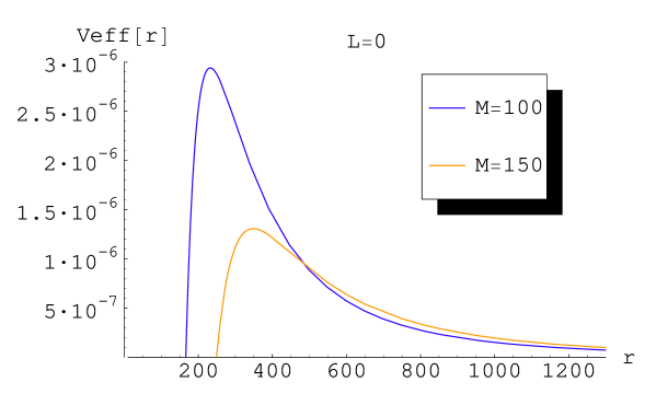
Figure 1: Effective potential of L=0 scalar modes for Semiclassical black hole with $M=100$(top curve) and $M=150$(bottom curve). $Q/M=0.75$ and the mass parameter of the quantum scalar field is chosen to be m=1/10.

As we can see in diagram (1), the effective potential $V$ has the form of a definite positive potential barrier, i.e, it is a well behaved function that goes to zero at spatial infinity and gets a maximum value near the event horizon. The quasinormal modes are solutions of the wave equation (17) with the specific boundary conditions requiring pure out-going waves at spatial infinity and pure in-coming waves on the event horizon. Thus no waves come from infinity or the event horizon. The quasinormal frequencies are in general complex numbers, whose real part determines the real oscillation frequency and the imaginary part determines the damping rate of the quasinormal mode. In order to evaluate the quasinormal modes for the test scalar field, we use the well known WKB technique, that can give accurate values of the lowest ( that is longer lived ) quasinormal frequencies. The first order WKB technique was applied to finding quasinormal modes for the first time by Shutz and Will shutz-will . Latter this approach was extended to the third order beyond the eikonal approximation by Iyer and Will iyer-will and to the sixth order by Konoplya konoplya2 .

We use in our numerical calculation of quasinormal modes this sixth order WKB expansion, for which was shown in konoplya3 that gives a relative error which is about two order less than the third WKB order. The sixth order WKB formula can be written as

$$i\frac{\left(\omega^{2}-V_{0}\right)}{\sqrt{-2V_{0}^{{}^{\prime\prime}}}}-\sum_{j=2}^{6}\Pi_{j}=n+\frac{1}{2},\ \ \ \ \ n=0,1,2,...$$ (22)

where $V_{0}$ is the value of the potential at its maximum as a function of the tortoise coordinate, and $V_{0}^{{}^{\prime\prime}}$ represents the second derivative of the potential with respect to the tortoise coordinate at its peak. The correction terms $\Pi_{j}$ depend on the value of the effective potential and its derivatives ( up to the 2i-th order) in the maximum ( see zhidenkothesis and references therein ). The above formula was used in several papers for the determination of quasinormal frequencies in a variety of systems WKB6papers . Yet one should remember that strictly speaking the WKB series converge only asymptotically and the consequence decreasing of the relative error in each WKB order is not guaranteed. Fortunately, in the considered case here, WKB series shown convergence in all sixth orders.

In the following we show the results for the numerical evaluation of the first two fundamental quasinormal frequencies considering a minimal coupling between the quantum field and the bare black hole. As we can see for the above expressions for the effective potential of the semiclassical black hole, the parameters entering in the determination of the quasinormal frequencies are the black hole bare charge $Q$ and mass $M$, the coupling constant $\xi$ between the quantum scalar and the classical gravitational fields, and the quantum field mass $m$. In table (1) we list values for the real and imaginary parts of the quasinormal frequencies for semiclassical and classical black holes varying the multipolar number $L$ and the overtone number $n$. The numerical results are obtained for minimal coupling between the quantum field and the background gravity field, fixing the bare black hole charge to mass ratio, and allowing to variation in $M$. The quantum scalar field mass is fixed taking into account the condition for the validity of the Schwinger-DeWitt approach.

Semiclassical solution				Classical solution
$M=100$
$L$	$n$	$Re(\varpi)$	$-Im(\varpi)$	$L$	$n$	$Re(\varpi)$	$-Im(\varpi)$
$0$	$0$	2.3302	1.2140	$0$	$0$	14.233	1.0638
$1$	$0$	3.5226	1.1772	$1$	$0$	3.8461	1.1606
$1$	$1$	3.1836	3.6897	$1$	$1$	8.1164	2.4344
$M=110$
$L$	$n$	$Re(\varpi)$	$-Im(\varpi)$	$L$	$n$	$Re(\varpi)$	$-Im(\varpi)$
$0$	$0$	1.2090	1.1042	$0$	$0$	6.0223	0.9657
$1$	$0$	3.2054	1.0698	$1$	$0$	3.4741	0.9579
$1$	$1$	2.8942	3.3544	$1$	$1$	5.1130	1.5760
$M=150$
$L$	$n$	$Re(\varpi)$	$-Im(\varpi)$	$L$	$n$	$Re(\varpi)$	$-Im(\varpi)$
$0$	$0$	1.0230	0.9337	$0$	$0$	2.1751	0.8333
$1$	$0$	2.7123	0.9053	$1$	$0$	2.9588	0.8928
$1$	$1$	2.4490	2.8383	$1$	$1$	6.2429	1.8724

Table 1: Rescaled Scalar quasinormal frequencies $\varpi=10^{3}\omega$ for the classical and semiclassical Reissner-Nordström black hole, with $Q/M=0.75$, $m=1/10$ and $\xi=0$.

As the obtained numerical results show, a shift in the quasinormal spectrum due to semiclassical corrections of the Reissner-Nordström background appears, an effect that is more pronounced for the fundamental mode $(L=0)$. From (2) and (3) we see that the backreaction of the quantized field upon the classical solution gives rise to a decreasing of the real oscillation frequencies and to a small decreasing of the damping rate, for physically interesting values of the black hole mass. Using the numerical results above presented, it is simple to see that, as a consequence of the vacuum polarization effect, we have an effective decreasing of the quality factor, proportional to the ratio $\frac{\left|Re(\omega)\right|}{\left|Im(\omega)\right|}$. As expected, the differences in the quasinormal frequencies when the black hole mass increases tend to disappear.

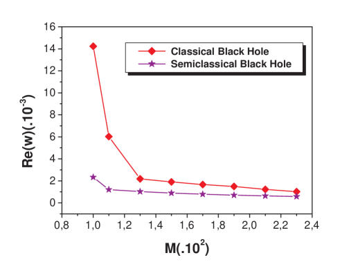
Figure 2: Dependance of $Re(\omega)$ on M for classical and semiclassical black holes. The parameters are chosen to be $Q/M=0.75$, $m=1/10$, $\xi=0$, $L=0$ and $n=0$.

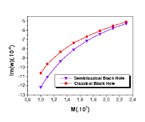
Figure 3: Dependance of $Im(\omega)$ on M for classical and semiclassical black holes. The parameters are chosen to be $Q/M=0.75$, $m=1/10$, $\xi=0$, $L=0$ and $n=0$.

From the above results, we arrive to the conclusion that the classical Reissner-Nordström black holes are better oscillators than its quantum corrected partners. This is in contrast with the results obtained by Konoplya in reference konoplyabtz for the BTZ black hole dressed by a quantum conformal massless scalar field. In that case was shown that the backreaction of the Hawking radiation increases the quality factor for semiclassical BTZ black holes in the small mass regime. The investigation of a similar problem (i.e, the increasing of the quality factor due to Hawking radiation, in contrast with the decreasing of that magnitude due to vacuum polarization ) for semiclassical charged black holes is in progress, and will be the subject of future publication by us.

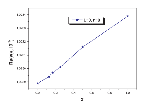
Figure 4: Behaviour of the real part of the quasinormal frequencies of the fundamental mode for different values of couplig constant $\xi$. In the figure $M=100$, $Q/M=0.75$,$m=1/10$.

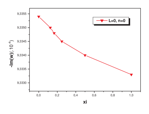
Figure 5: Behaviour of the imaginary part of the quasinormal frequencies of the fundamental mode for different values of couplig constant $\xi$. In the figure $M=100$, $Q/M=0.75$,$m=1/10$.

We also evaluate the dependence of the quasinormal frequencies for a given black hole bare mass and different values of the coupling constant between the quantum field of fixed mass $m$ and the classical background spacetime, including the more physically interesting cases of minimal and conformal coupling . The results appears in figure (4) and (5). As we can see, the quasinormal frequencies shows only a little dependance on the coupling constant. As the coupling constant increases, we see an almost linear small increment in the real and imaginary parts of the quasinormal frequencies for semiclassical black holes. A similar very small effect appears if we consider the dependance of the quasinormal frequencies on the mass of the quantum scalar field, for a fixed bare black hole mass and coupling constant. As the quantum field mass increases, we found a very little increment in the real part of the frequencies for semiclassical black holes, and a very little decreasing in the imaginary part. Therefore, the shift in the quasinormal frequencies with respect to the classical bare black hole appears to be almost the same for the given range of the quantum field parameters.

V Concluding remarks

We have studied the influence of the backreaction due to vacuum polarization on the structure of test scalar quasinormal frequencies for semiclassical charged black holes. The semiclasical solution studied describes a Reissner-Nordström black hole dressed by a quantum massive scalar field in the large mass limit. Such an influence appears essentially as an appreciable shift in the quasinormal frequencies that decreases as the bare black hole mass increases, and that not have a strong dependance upon the quantum field parameters. This shift shows that the quantum corrected quasinormal modes are less oscillatory with respect to its classical counterpart. The new features mentioned above regarding the quasinormal frequencies of the semiclassical solution so far reflect the physics of the back reaction of a single specie of a field of spin $s=0$. While this have revealed novel important features of the quasinormal ringing stage for the quantum corrected black hole considered, a more realistic setting should take into account black holes surrounded by the multiple species of quantum fields, belonging to the Standard Model. It is expected that the shifts in the frequency spectrum obtained in this case should be more appreciable than in the situation considered in this work. The results for this more realistic case will be presented in a forthcoming paper.

VI Acknowledgements

This work has been supported by FAPESP and CNPQ, Brazil as well as ICTP, Trieste. We are grateful to Professor Elcio Abdalla for the useful suggestions. One of the authors (J. de Oliveira) ought to express his gratitude by the kind hospitality granted by the Departamento de Física y Química at the University of Cienfuegos, Cuba, where this work was realized. O.P. F. Piedra also thanks to Owen Daniel Fernández Chacón, for his help in preparing the figures, and to Dr. Alexander Zhidenko, for provide valuable information about numerical methods usually employed in the calculation of quasinormal frequencies.

References

- (1) E. Berti, V. Cardoso, J. P. S. Lemos, Phys. Rev. D70, 124006 (2004).
- (2) K. D. Kokkotas, D. G. Schmidt, Liv. Rev. Relat. 2, 2 (1999).
- (3) E. W. Leaver, Phys. Rev. D45, 4713 (1992); C. Gundlach, R. H. Price, J. Pullin, Phys. Rev. 49, 883 (1994); E. Abdalla, R. A. Konoplya, C. Molina, Phys. Rev. D72, 084006 (2005).
- (4) V. Cardoso, J. P. S. Lemos, Phys. Rev. D67, 084020 (2003); R. A. Konoplya, A. Zhidenko, JHEP 0406, 037 (2004); R. A. Konoplya, Phys. Rev. D68, 124017 (2003).
- (5) B. Wang, C. Y. Lin, E. Abdalla, Phys. Lett. B481, 79 (2000); B. Wang E. Abdalla, C. Molina, Phys. Rev. D63, 084001 (2001); C. Molina, D. Giugno, E. Abdalla, A. Saa, Phys. Rev. D69, 104013 (2004); E. Abdalla, B Cuadros Melgar, C. Molina, A. Pavan, Nucl. Phys. B752, 40 (2006).
- (6) H. P. Nollert, Class. Quant. Grav. 16, R159 (1999).
- (7) G. T. Horowitz, V. E. Hubeny, Phys. Rev. D62, 024027 (2000).
- (8) A. S. Miranda, J. Morgan and V. T. Zanchin, JHEP 0811 (2008) 030.
- (9) R. A. Konoplya, Phys. Rev. D70, 047503 (2004).
- (10) R. A. Konoplya, Phys. Rev. D68, 024018 (2003);R. A. Konoplya, Phys. Rev. D68, 124017 (2003).
- (11) N.D. Birrel and P. C. Davies, Quantum Fields in Curved Space , (Cambridge University Press, Cambridge, 1982) .
- (12) P. R. Anderson, W. A. Hisckock and D. A. Samuel, Phys. Rev. D51, 4337 (1995).
- (13) L. P. Grischuk, Zh. Eksp. Teor. Fiz 67, 825 (1974)[Sov. Phys. JETP 40, 409 (1975)].
- (14) J. W. York, Phys. Rev. D31, 775 (1985), D. Page, Phys. Rev. D25, 1499 (1982).
- (15) D. Page, Phys. Rev. D25, 1499 (1982).
- (16) V. P. Frolov and A. I. Zelnikov, Phys. Lett. 115B, 372 (1982), V. P. Frolov and A. I. Zelnikov, Phys. Lett. 123B, 197 (1983), V. P. Frolov and A. I. Zelnikov, Phys. Rev. D29, 1057 (1984); A. O. Barvinsky and G. A. Vilkovisky, Phys. Rept. 119, 1 (1985).
- (17) I. G. Avramidi, Nucl. Phys. B355, 712 (1991), I. G. Avramidi, PhD Thesis, hep-th/9510140.
- (18) J. Matyjasek, Phys. Rev. D61, 124019 (2000) .
- (19) J. Matyjasek, Phys. Rev. D63, 084004 (2001) .
- (20) A. O. Barvinsky and G. A. Vilkovisky, Phys. Rept. 119, 1 (1985) .
- (21) B. S. DeWitt, Phys. Rept 53, 1615 (1984) .
- (22) V. P. Frolov and A. I. Zelnikov, Phys. Lett. 123B, 197 (1983), V. P. Frolov and A. I. Zelnikov, Phys. Rev. D 29, 1057 (1984).
- (23) C. W. Misner, K. S. Thorne and J. A. Wheeler, Gravitation, ( Freeman, San Francisco, 1973).
- (24) Owen Pavel Fernández Piedra and Alejandro Cabo Montes de Oca, Phys. Rev. D75, 107501 (2007) .
- (25) Owen Pavel Fernández Piedra and Alejandro Cabo Montes de Oca, Phys. Rev. D77, 024044 (2008) .
- (26) Owen Pavel Fernández Piedra and Alejandro Cabo Montes de Oca, gr-qc/0701135.
- (27) B. S. DeWitt, Phys. Rept 53, 1615 (1975); P. B. Gilkey, J. Diff. Geom. 10, 601 (1975) .
- (28) Y. Decáninis and A. Folacci, Class. Quantum Grav. 24, 4777 (2007).
- (29) W. Berej and J. Matyjasek, Acta. Phys. Pol. B34, 3957 (2003).
- (30) B. E. Taylor, W. A. Hisckock and P. R. Anderson, Phys. Rev. D61, 084021 (2000).
- (31) C. O. Loustó and N. Sanchez, Phys. Lett. 212B, 411 (1988).
- (32) B. Shutz and C. M. Will, Astrophys. J. Lett. L33, 291 (1985).
- (33) S. Iyer and C. M. Will, Phys. Rev. D35, 3621 (1987).
- (34) R. A. Konoplya, J. Phys. Stud. 8, 93 (2004).
- (35) A. Zhidenko, PhD Thesis, arxiv:0903.3555.
- (36) R. A. Konoplya and E. Abdalla, Phys. Rev. D71, 084015 (2005); E. Abdalla, O. P. F. Piedra and J. de Oliveira, arxiv:0810.5489;M.I. Liu, H. I. Liu and Y. X. Gui, Class. Quantum Grav. 25, 105001 (2008);P. Kanti and R. A. Konoplya, Phys. Rev. D73, 044002 (2006); J. F. Chang, J. Huang and Y. G. Shen Int. J. Theor. Phys. 46, 2617 (2007); H. T. Cho, a. S. Cornell, J. Doukas and W. Naylor, Phys. Rev. D77, 016004 (2008); J. F. Chang and Y. G. Shen Int. J. Theor. Phys. 46, 1570 (2007); Y. Zhang and Y. X. Gui, Class. Quantum Grav. 23, 6141 (2006); R. A. Konoplya Phys. Lett. B550, 117 (2002); S. Fernandeo and K. Arnold, Gen. Rel. Grav. 36, 1805 (2004); H. Kodama, R. A. Konoplya and A. Zhidenko, arxiv:0904.2154; H. Ishihara, M. Kimura, R. A. Konoplya, K. Murata, J. Soda and A. Zhidenko, Phys. Rev. D77, 084019 (2008); R. A. Konoplya and A. Zhidenko, Phys. Lett. B644, 186 (2007); R. A. Konoplya, arxiv: 0905.1523; H. Kodama, R. A. Konoplya and A. Zhidenko, arxiv: 0904.2154;